




No CrossRef data available.
Article contents
CONDITIONAL INFERENCE FOR POSSIBLY UNIDENTIFIED STRUCTURAL EQUATIONS
Published online by Cambridge University Press: 04 August 2003
Abstract
The possibility that a structural equation may not be identified casts doubt on measures of estimator precision that are usually used. Using the Fieller–Creasy problem for illustration, we argue that an observed identifiability test statistic is directly relevant to the precision with which the structural parameters can be estimated, and hence we argue that inference in such models should be conditioned on the observed value of that statistic (or statistics).
We examine in detail the effects of such conditioning on the properties of the ordinary least squares (OLS) and two-stage least squares (TSLS) estimators for the coefficients of the endogenous variables in a single structural equation. We show that (a) conditioning has very little impact on the properties of the OLS estimator but a substantial impact on those of the TSLS estimator; (b) the conditional variance of the TSLS estimator can be very much larger than its unconditional variance (when the identifiability statistic is small) or very much smaller (when the identifiability statistic is large); and (c) conditional mean-square-error comparisons of the two estimators favor the OLS estimator when the sample evidence only weakly supports the identifiability hypothesis but favor TSLS when that evidence moderately supports identifiability.
Finally, we note that another consequence of our argument is that the statistic upon which Anderson–Rubin confidence sets are based is in fact nonpivotal.We are grateful for the constructive comments offered by Peter Phillips and three anonymous referees that greatly improved the paper. Giovanni Forchini acknowledges support from ESRC grant NR00429424115.
Information
- Type
- Research Article
- Information
- Copyright
- © 2003 Cambridge University Press
1. INTRODUCTION
A niggling concern for econometricians for many years has been the possibility that structural models may not be identified (Sims, 1980; Sargan, 1983) or may be only partially identified (Phillips, 1989) or may involve “weak instruments” (Nelson and Startz, 1990; Dufour, 1997; Staiger and Stock, 1997). Recent literature on both exact distribution theory and asymptotics for this model suggests that this concern is fully justified from a frequentist point of view. The work of Chao and Phillips (1998) and Kleibergen and van Dijk (1998) shows that it is also justified in a Bayesian analysis of the model, although in this paper we shall be concerned only with a frequentist approach.
The work of Phillips (1983, 1989) and Hillier (1985, 1990) has made it clear that if the exclusion restrictions imposed on (the exogenous variables in) the structural equation are spurious (i.e., the structural equation is totally unidentified), then the densities of the ordinary least squares (OLS), two-stage least squares (TSLS), and limited information maximum likelihood (LIML) estimators of the coefficients of the endogenous variables depend only on the error covariance matrix, and not on the structural parameters, so that none of these statistics contains information about those parameters. Because also standard asymptotic theory breaks down when the model is unidentified, identification must be presumed if these statistics are to be interpreted as useful estimators.
Motivated by such concerns, recent literature on the distributions of the TSLS and LIML estimators has started to focus on intermediate situations where the equation of interest is neither formally identified nor totally unidentified. To bridge the gap, Phillips (1989) has introduced the idea of partially identified models. These are models for which some, but not all, of the parameters are identified after a rotation of coordinates in the space of both the endogenous and exogenous variables. Choi and Phillips (1992) have found that in such models the distributions of the usual estimators of both the identified and the unidentified coefficients of the endogenous variables are mean- and covariance-matrix mixed-normal. Although the density of the estimator of the unidentified parameters does not depend on the unidentified parameters, it does depend on the identified parameters. The estimator of the identified parameters is consistent, but conventional asymptotics does not apply. Moreover, the estimator of the unidentified parameters converges in law to a nondegenerate, nonstandard distribution.
In a different attempt to study intermediate cases Staiger and Stock (1997) define a notion of weakly identified models. Such models have two characteristics: they are formally identified for all finite sample sizes, but the covariance between the instruments and the included endogenous variables is assumed to be in a O(T−1/2) neighborhood of zero, where T is the sample size. Staiger and Stock (1997) show that standard asymptotics fails for such models and that the asymptotic distributions of the usual estimators have the same structure as their exact distributions under normality (i.e., mixed-normal). These results lead Staiger and Stock to stress the importance of reporting the test statistic for identification, but they do not indicate how the value of that statistic should modify inference, if at all. Hall, Rudenbusch, and Wilcox (1996) also stress the importance of such an identification test statistic. More recently, Stock and Yogo (2001), in a paper discussing the meaning and measurement of the weak instrument concept, arrive at precisely the same statistic as we do but again only as a test for weak instruments.
A related recent development is based on the observation that inference on structural parameters is essentially a generalization of the Fieller–Creasy problem (see Wallace, 1980). Scheffé (1970) defines a confidence set as improper if it has positive probability of being the entire parameter space. In the Fieller–Creasy problem, this probability corresponds to the probability that the identifiability test statistic is small. Generalizing Koschat (1987) and Gleser and Hwang (1987), Dufour (1997) has shown that in a potentially unidentified structural model valid confidence sets must be improper in Scheffé's sense and argues in favor of Anderson-Rubin-type (Anderson and Rubin, 1949) confidence sets (a generalization of the Fieller–Creasy solution). Zivot, Startz, and Nelson (1998) provide a further analysis of this problem for the structural model, again emphasizing the role of an identifiability test statistic. Both Hall et al. (1996) and Zivot et al. (1998) find that, although the identification test statistic is crucial, using it to “pretest” for identifiability cannot be recommended. It is important to note that, in all of this work, “potentially unidentified” really means that, although the model may be formally identified, it is impossible to rule out a priori models that are arbitrarily close to being unidentified.
In this paper we argue that the correct way to take account of the possibility that such a model may be formally unidentified, or arbitrarily close to being so, is to explicitly take account of the sample evidence on the identification of the model by conditioning on an identifiability test statistic (or statistics). In particular, we argue that the reported precision of parameter estimates should be that in the conditional distribution of the estimator given the observed value of an identifiability test statistic and not the unconditional precision. The analysis is exact rather than asymptotic and supplements the work of Staiger and Stock (1997) by suggesting exactly how the identifiability test statistic should affect inference procedures for these models. Crucially, in our analysis, inferential procedures depend continuously on the identifiability test statistic, rather than discontinuously as is the case in the “pretesting” approach mentioned previously.
The paper is organized as follows. The crux of the paper is the argument that, in inference problems of this type, conditional measures of estimator precision are more relevant than unconditional measures. For expositional purposes we use the Fieller–Creasy problem as a model for this argument and only later (in Section 3) apply it to the more complex problem of structural estimation. The essence of the argument is that both of these inference problems can be embedded in models for which no inference problem arises and that the key to the difficulty lies in the properties of the mapping defining the interest parameter(s) in terms of the parameters of the embedding model. The main argument is presented in Section 2.
In Section 3 we introduce the structural model and generalize the key parts of the argument from Section 2 to this more complicated case. In Section 4 we present exact conditional results for the OLS and TSLS estimators of the coefficients of the endogenous variables, and we give new measures of the precision of these estimators that properly reflect the possibility that the model may not be identified. Among our conclusions in this section is the fact that the conditional density of the OLS estimator is quite insensitive to the identifiability statistic, whereas that of the TSLS estimator is sensitive to it. Thus, OLS can conditionally dominate TSLS, or vice versa, depending on the data actually obtained. Clearly, this conclusion, and its implications for applied work, is quite at odds with received opinion on inference procedures for the structural model. Finally, in Section 5 we discuss Fieller's solution to the inference problem for a ratio of normal means and discuss its analogue in the structural model, Anderson–Rubin confidence sets, in the light of what has come before. Here we argue that in each case the statistic used to construct the confidence set is, contrary to popular belief, nonpivotal.
All of our results for the structural model are derived under classical assumptions of normal errors and no lagged endogenous variables. In this restricted context they are exact, but they can also be thought of (with suitable definitions of the key parameters involved) as paradigms for the asymptotic results that would apply for much more general models (see, e.g., Phillips, 1989; Choi and Phillips, 1992; Staiger and Stock, 1997). Also, much of our argument evidently has applications in the context of error-correction time series models, where rank conditions play a crucial role for both estimation and testing, but this extension of the argument is not developed in the present paper.
2. THE ARGUMENT FOR CONDITIONING
2.1. Conditioning: Postdata Precision
Reporting the results of an inference procedure, whether it be inference about the values of unknown parameters or a decision about whether certain propositions of interest about the model under study seem correct or false, entails two inter-related components: reporting the results of the procedure as applied to the data at hand and reporting some measure of the likely precision that can be attributed to those results. For a Bayesian, these two objectives are met (at least in principle) by reporting the posterior distribution or some of its key features. For the frequentist precision is usually indicated by reporting a confidence set for the parameter(s) of interest, together with its confidence level, or by reporting the variance or mean-square error of the estimator chosen, or approximations to them.
For the Bayesian, of course, inference is conditioned on the full sample, so that estimator “precision,” by construction, depends fundamentally on the data actually observed. In contrast, standard frequentist measures of the precision of an inference have, until recently, relied entirely on predata assessments of the procedure used, obtained by averaging (some relevant property of the procedure) over the entire sample space. But, as Lindsay and Li (1997) remark: “After the data is observed, however, the actual ‘postexperimental’ error associated with that particular sample becomes more relevant.” Thus, for an estimation problem: “the average error is an attribute of an estimator, … , whereas the postexperimental error is an attribute of an estimate.” (For a recent discussion, see also Goutis and Casella, 1995.) The suggestion implicit here is that certain features of the sample actually obtained may be pertinent to the assessment of the precision of the estimate but of course are immaterial to the predata (average) properties of the estimator. In what follows we adopt an entirely frequentist approach but will argue that, for inference problems of the type considered, the relevant measures of estimator precision are conditional measures.
Any attempt to assess the likely precision of an estimate—that is, to assess the likely precision of the procedure in the sample actually available—clearly must involve some sort of averaging process but, equally, must hold certain aspects of the sample actually used fixed. In other words, whatever precision measure is used, it must, if it is to measure a property of the estimate (rather than the estimator) be conditional on certain aspects of the sample remaining fixed at their observed values. Thus, any postdata measure of the precision of an estimate must be conditional. The problem, both in practice and from a philosophical point of view, is precisely what to condition on. That is, how can one identify events that are pertinent to the precision achieved by an inference procedure?
The only situations in which there seems to be widespread agreement among (frequentist) statisticians—both that conditioning is sensible and upon what to condition—are those in which there is an exact ancillary statistic (cf. Cox, 1958; Efron and Hinkley, 1978; Barndorff-Nielsen, 1980). This agreement is almost certainly attributable to the fact that, under suitable assumptions, it is straightforward to show that the Fisher information based on the conditional distribution of (say) the maximum likelihood estimator given the ancillary is identical to that of the full sufficient statistic, whereas the marginal density of the estimator must yield smaller Fisher information. That is, conditioning on the ancillary recovers information that would otherwise be lost. Even here the problem is difficult (see the collected papers by D. Basu edited by Ghosh, 1988), and outside this fairly narrow class of problems study of the problem has barely begun. Notice, though, that the argument for conditioning rests not on the ancillarity of the conditioning statistic per se but rather on a concern—similar to that expressed by Lindsay and Li—to obtain a more relevant measure of the inferential precision actually achieved in the sample (see also Barndorff-Nielsen's comments on the paper by Efron and Hinkley, 1978; and the discussion in Cox and Hinkley, 1974, Ch. 2). For related work explicitly concerned with confidence sets and hypothesis testing see Kiefer (1977), Hwang and Brown (1991), and Hwang, Casella, Robert, Wells, and Farrell (1992).
We do not intend to enter into the wider debate on these issues here. However, we shall advocate, for a particular class of problems to be described shortly, conditional measures of precision—and for precisely the reason that applies in the wider problem: to obtain a more relevant measure of the precision achieved in the sample actually available. As noted previously, the problem is to identify aspects of the data that are pertinent to the precision of the estimate, and we shall argue that, in the types of models we are considering, the structure of the problem clearly identifies which events affect precision. We begin by discussing the simplest possible example of the type of problem we shall be concerned with—the Fieller–Creasy problem.
2.2. The Fieller–Creasy Problem
The Fieller–Creasy problem is a celebrated, apparently straightforward, inference problem that produces “paradoxical” assessments of precision, namely, improper confidence sets (for a historical survey of the problem, see Wallace, 1980). The problem contains virtually all the essential features of the structural model that is our main concern and is also closely related to the linear calibration (inverse regression) problem (Hoadley, 1970; Dobrigal, Fraser, and Gebotys, 1987; Gleser and Hwang, 1987), errors-in-variables regression, some principal component inference problems, and inference on ratios of regression parameters.
Assume that the 2 × 1 vectors xi(i = 1,…,T) are independent N(μ, σ2I2) and that we are interested in either the ratio of means ψ = μ1 /μ2 or in the direction of the vector μ, parameterized by the angle, φ, when μ is expressed in polar coordinates in the usual way. The vector of sample means, x, and

are jointly sufficient for (μ,σ2), x ∼ N(μ,(σ2/T)I2), x is independent of s2, and s2/σ2 ∼ χ2(2(T − 1)). The maximum likelihood estimator for ψ is

, but the (unconditional) variance of

does not exist. Fieller (1954) and Creasy (1954) consider the problem of constructing a confidence interval for ψ, and the standard “Fieller solution” is based on the observation that, when μ2 ≠ 0,

where

. However, this solution entails the “paradox” that the confidence interval it produces is
(a) the entire real line if

, where Fα(ν1,ν2) is such that Pr{F(ν1,ν2) < Fα(ν1,ν2)} = 1 − α,
(b) the interior of a finite interval if x22 > c, and
(c) the exterior of a finite interval if ∥x∥2 > c and x22 < c.
Thus, it is entirely possible for, say, the 90% confidence interval for ψ to consist of the whole real line, and the (unconditional) expected length of the interval is infinite.
Scheffé (1970), James, Wilkinson, and Venables (1974), Dobrigal et al. (1987), and Koschat (1987) all treat the problem in terms of the interest parameter φ, rather than ψ. Essentially the same paradox arises although, as we shall see, there is a subtle difference between the two versions of the problem.
Koschat (1987), for this problem, and Gleser and Hwang (1987), for a wider class of closely related problems, have shown that problems of this type have the property that every confidence set with nonzero confidence coefficient must have positive probability of being the entire parameter space and hence must be improper in the sense of Scheffé (1970). Hence, the difficulty is not peculiar to the Fieller solution. Dufour (1997) has extended these results to the structural model and other models of interest in econometrics.
2.3. Interest Parameters and Critical Sets
Now, notice that in the preceding Fieller problem, there is certainly no difficulty in obtaining an always-bounded confidence set for the underlying parameter vector μ. The region (sphere) defined by the acceptance region for a likelihood ratio test,

is the most obvious candidate. Apart from being (equivalent to) the likelihood ratio statistic, F is the (unique) maximal invariant under the group of transformations G = {(a,H),a > 0,H(2 × 2) orthogonal} acting on the variates (x − μ,s2) by

Thus, confidence regions for μ based on F characterize the entire class of invariant regions.
The important point about the regions (2) is that the Fieller problem is naturally embedded in a model for which no paradox arises, because the region (2) is bounded with probability one. That is, the “Fieller paradox” derives from the properties of the mapping

and not from any intrinsic property of the embedding model. We shall see shortly that this observation also applies to the structural model, but before doing so we elaborate on its implications for the Fieller problem itself, where the situation is simpler.
If γ = γ(μ) is an everywhere continuous one-to-one function of μ, the image of any closed bounded set of μ-values is a closed bounded set of γ-values, so that the (proper) confidence set (2) for μ naturally induces a proper confidence set for γ (with the same confidence level). In this sense, inferential results for μ are sufficient for inference about any everywhere continuous and one to one function of μ, and it seems reasonable to assert that, in these circumstances, there is no essential difference between the inference problem for μ and that for (any such function) γ. Of course, actual measures of precision, like estimator variances, or Fisher information, change under reparameterization, but, although seldom stated explicitly, estimator loss functions would usually embody exactly this invariance under smooth reparameterizations, so in a more formal decision-theoretic treatment of the estimation problem this property would emerge naturally.
On the other hand, the key characteristic of (both versions of) the Fieller problem is that the mapping from the underlying parameter μ to the interest parameter ψ (or φ) is not everywhere continuous and one-to-one. In the case of the interest parameter ψ, the mapping μ → (ψ,μ2) (from

) is continuous and one-to-one everywhere except along the μ1 axis, where ψ can take any value. In the case of the interest parameter φ, the mapping μ → (φ,ρ) (where ρ = ∥μ∥) is continuous and one-to-one everywhere except at the origin (μ = 0), where φ can take any value. Dufour (1997) calls such subsets of the parameter space nonidentification subsets, but we shall refer to them as critical sets. Notice that the critical set depends on the definition of the interest parameter(s) in terms of the parameters of the embedding model.
The Fieller solution (1) is easily obtained from (2). The line μ1 − ψμ2 = 0 intersects the sphere ∥x − μ∥2 < f just if (x1 − ψx2)2/(1 + ψ2) < f. The induced (Fieller) confidence set for ψ is thus the set for which this line intersects the sphere, and is a finite interval if the sphere does not cross the μ1-axis (i.e., x22 > f), is the exterior of a finite interval if the sphere crosses the μ1 axis but does not include the origin, (i.e., x22 < f but ∥x∥2 > f), and is the entire real line if the sphere contains the origin (i.e., ∥x∥2 < f). It is clear, too, that for either version of the Fieller problem, the region (2) must intersect the critical set for some values of (x,s2) unless it has confidence level zero. That is, every confidence set for ψ (or φ) induced by (2) must be improper unless it has confidence level zero.
We now generalize these observations on the Fieller problem to an arbitrary model in which the interest parameter can take any value on a subset of the full parameter space for the embedding model.
Postdata precision.
Generalizing the Fieller problem, let p(x;θ) denote the model density for either the sample data or the minimal sufficient statistic, with

. In general an interest parameter can be defined as some functional defined on the family of densities P = {p(x;θ);θ ∈ M} (see Pfanzagl, 1998), and the critical set (if, for the given interest parameter, there is one) is then the subset of P on which this functional fails to be continuous. For the problems we are concerned with here it suffices to consider reparameterizations

with the property that the interest parameter γ1 can take any value on some subset C of M. We call C the critical subset of M (for the interest parameter γ1). Note that membership of C is an attribute of θ, not of γ1. Let

denote the maximum likelihood estimator (MLE) for θ and let

denote the confidence set for θ based on the acceptance region for a likelihood ratio test (of the simple hypothesis H0 : θ = θ). The confidence level is determined by the choice of c, with smaller values of c corresponding to larger confidence levels.
In practice the interest parameter may be defined in terms of some subset of the full parameter vector θ. If so, LRc(x) must be modified by replacing the numerator by its maximum value over parameters not involved in the definition of γ1 and replacing the denominator by its maximum over the values of all parameters. For expository purposes we work with the simplest case. We assume that the regions (3) are bounded with probability one. Obviously, the acceptance region based on any testing principle could be used in place of (3), with obvious modifications to the argument that follows.
For fixed data x, and a fixed critical set C, two extreme cases of (3) can occur:
(a) LRc(x) intersects C for all, or all but very large, values of c. That is, LRc(x) is “close to” C for all but very large values of c. In this case the induced confidence region for γ1 will be unbounded for all but very small confidence levels, and it seems reasonable to conclude that, with the particular data x, γ1 is determined with “low precision”;
(b) LRc(x) and C may be disjoint for all but very small values of c (of course, they cannot be disjoint for all c if C is nonempty). That is, LRc(x) is “remote from” C for all but very large confidence levels. In this case it seems reasonable to conclude that, with these particular data x, γ1 is determined with “high precision.”
If we take as given the standard (frequentist) position that confidence sets are an adequate, if somewhat philosophically problematic, representation of the precision of an inference, these remarks suggest that the location of LRc(x) in relation to the critical set C has, for problems of this type, a direct bearing on the precision with which γ1 can be learned from the data available. Moreover, they suggest an intuitively reasonable measure of how accurately γ1 can be determined with the data available, namely:

where c0 is the smallest value of c in (3) for which LRc(x) does not intersect C. For, if c0 is near one only very “small” regions (i.e., low confidence levels) for θ would be compatible with a nontrivial region for γ1 (with the given data), and this indicates low precision in the ability of the data to inform about γ1, whereas c0 near zero would mean that very large likelihood ratio confidence regions (with high confidence levels) would be (with these data) compatible with a nontrivial interval for γ1.
Remarks.
1. If C is empty, so that the mapping θ → γ is everywhere continuous and one-to-one, c0 = 0, because LRc(x) can be made as large as we like without intersecting C. Thus, in this case, κ = 1 for any x, and the precision with which any everywhere one to one function of θ can be located is identical to that with which θ itself can be located, as is natural.
2. If, with the data available, LRc(x) intersects C for all c, c0 = 1, and κ = 0, indicating that, with these data, there is no prospect of locating γ1.
3. The confidence set for θ based on the likelihood ratio in (3) has the advantage that different choices for the mapping θ → γ that leave the interest parameter γ1 invariant will leave κ invariant.
4. κ is evidently a monotonic increasing function of the maximum confidence level (for likelihood ratio based confidence sets for θ) that (with the given data) is compatible with a nontrivial confidence set for the interest parameter γ1. This maximum confidence level (mcl) could itself be used as an index of precision (see Table 1).
5. The precision for inference about the interest parameter, γ1, has been defined so as to depend on the entire vector θ, because membership of the critical set C is an attribute of θ, not γ1. In this respect κ reflects information in the data about both “nuisance parameters” and the “interest parameter.” This, it seems to us, is natural when the true source of the inference problem has been recognized.
6. Because, under regularity conditions, the power of the likelihood ratio test goes to unity as T → ∞, it is clear from (4) that, provided θ ∉ C, κ → 1 in probability as T → ∞. That is, the precision with which γ1 can be located will, if θ ∉ C, approach one as the sample size increases. Just as important, the converse is also easily seen to be true: if θ ∈ C, the precision index, κ, goes to zero in probability as T → ∞.
Precision indices and maximum confidence levels

In both versions of the Fieller problem, the second component of the transformation μ → γ (in the first case, μ2, in the second, ρ) is constant (zero) on the critical set C. In the general case, the transformation θ → γ = (γ1,γ2) can usually be chosen so that γ2 vanishes on C. The implication of this remark, then, is that the “noninterest” parameter γ2 is, far from being a “nuisance parameter,” actually the key to the precision with which γ1 can be determined: it would be quite misleading to report precision measures for γ1 that did not depend on γ2, or on the sample evidence on the value of γ2. In fact—as we shall see shortly—this evidence is encapsulated in the precision index, κ.
Now, as initially defined, κ measures how remote (or otherwise) likelihood ratio based confidence regions for θ are from the critical set C. It is easy to see, however, that κ is completely determined by the likelihood ratio test statistic for testing the hypothesis H0 : θ ∈ C against an unrestricted alternative. For, denoting this test statistic by LR(C), we have

Hence, the postdata index of precision for γ1, as measured by κ(γ1; x), will be large just if the likelihood ratio test statistic for testing θ ∈ C is small (suggesting rejection) and vice versa.
Examples.
For the two versions of the Fieller–Creasy problem we have the following results.
1. Interest parameter ψ: In this case the critical set C = {μ : μ2 = 0}, and the region F < Fα in (2) intersects C unless

. For inference about the ratio of means, ψ,

Here, w1 is the usual test statistic for testing H0 : μ2 = 0, or μ ∈ C.
2. Interest parameter φ: Here C = {0}, and the region F < Fα in (2) intersects C unless

. For inference about the direction, φ, of μ,

Here, w2 is the usual test statistic for testing H0 : μ = 0, or μ ∈ C.
Note that, as one would expect, in both cases κ depends on the sample size, T. Clearly, κ differs in these two versions of the Fieller problem precisely because the interest parameter, and hence the critical set C, differs. Some values of the precision index κ for the Fieller problem with interest parameter ψ are given in Table 1. For example, if the observed value of w1 is 1, and T = 20, κ = 0.405, and the maximum confidence level (mcl) for which the confidence region (2) just intersects the μ1-axis is 0.389. Both numbers indicate that ψ would be poorly determined with such data.
The preceding argument establishes that, for any problem of the type we are interested in, the likelihood ratio test statistic for testing θ ∈ C, LR(C), is directly relevant to the precision with which, with the given data, the interest parameter γ1 can be located, from a frequentist point of view. Various other treatments of the problem can be interpreted as also leading to this conclusion (at least in the Fieller–Creasy and closely related problems). First, for the Fieller–Creasy problem (and hence the inverse linear regression/calibration problems), Hoadley (1970) has shown that LR(C) emerges naturally as an index of precision when the problem is viewed from a Bayesian perspective. In particular, under Hoadley's assumptions, the posterior density is more sharply peaked when the observed value of LR(C) is large. Second, using a fiducial argument, Dobrigal et al. (1987) suggest confidence sets (for the angle, φ, in the polar coordinate version of the Fieller problem) conditioned on the value of LR(C). The length of the interval suggested decreases with LR(C), but the interval is always bounded. Finally, it is not difficult to show that, for the Fieller problem in either form, the shape of the likelihood function near its maximum depends heavily on LR(C), so that adherents to the strict likelihood principle (including Edwards, 1972) would use LR(C) to indicate how accurately the MLE is determined. Thus, whatever one's statistical persuasions, for problems of this type the observed value of the likelihood ratio test statistic for testing H0 : θ ∈ C is directly relevant to the precision with which the data are revealing about the interest parameter γ1.
To summarize, we have argued that (a) inference problems, like the Fieller problem, and the structural equation model, can usually be embedded in a model for which no paradox arises; (b) the problem arises because the reparameterization involved in the definition of the interest parameter entails a critical set in the embedding parameter space on which the interest parameter can take more than one value; (c) the likelihood ratio test statistic for testing whether, in the embedding model, and with the data actually available, the parameter lies in the critical set, is a natural measure of the ability of the sample to inform about the interest parameter; (d) far from being a “nuisance,” the sample evidence on the noninterest parameter component of the reparameterized model is directly relevant to the precision with which the interest parameter itself can be located.
Our conclusion is that the observed likelihood ratio test statistic for testing membership of the critical set is directly relevant to the precision with which the interest parameter can be estimated with the data actually available and that it therefore makes no sense to average over values of that statistic that have not occurred. That is, we conclude that any sensible assessment of the properties of estimates of the interest parameter(s) must be made conditional on the observed value of such a test statistic (or other relevant indicators of critical set membership). In particular, estimator precision should be measured by the conditional variance or mean-square error (MSE), not the unconditional variance or MSE.
It should be remarked at this point that, because the preceding argument could be based on the confidence set produced by several tests, our argument does not, by itself, identify a unique conditioning statistic or a unique conditional measure of precision. The likelihood ratio statistic seems to us the most natural choice and has, of course, a number of well-known advantages. Nevertheless, in both the Fieller–Creasy problem and the structural model other possibilities may be worth investigating in future work.
It would be natural at this point to report the conditional density and variance (or MSE) of the MLE for ψ in the Fieller–Creasy problem, conditional on w1. However, these turn out to be a special case of the results that follow for the structural equation model, so we defer discussing them for the moment (see Remark 6 following Theorem 2 in Section 4).
3. THE STRUCTURAL EQUATION MODEL
We consider a single structural equation written without explicit normalization:

where Y = (y1,Y2) is a T × (n + 1) matrix of endogenous variables, Z1 is a T × k1 matrix of exogenous variables, and β[utri ] and γ are, respectively, (n + 1) × 1 and k1 × 1 vectors of parameters. The reduced form corresponding to (6) is

where Z2 is a T × k2 matrix of exogenous variables not included in the structural equation and Φ and Π are matrices of parameters of dimension k1 × (n + 1), k2 × (n + 1), respectively. We assume throughout that k2 ≥ n. The rows of V are assumed to be independent normal vectors with mean zero and common (n + 1) × (n + 1) covariance matrix

where ω11, ω21, and Ω22 are, respectively, (1 × 1), (n × 1), and (n × n) matrices of parameters. The reduced form (7), with the preceding assumptions, constitutes the embedding model for this problem.
Compatibility of the structural equation (6) and reduced form (7) requires the existence of some β[utri ] ≠ 0, such that

Φβ[utri ] = γ, Vβ[utri ] = u. Note that (8) implies rank(Π) ≤ n. If rank(Π) = n, equation (8) uniquely determines the direction of β[utri ] (i.e., β[utri ] is restricted to lie in a one-dimensional space). If rank(Π) < n, β[utri ] can be written as a linear combination of the n + 1 − rank(Π) basis vectors spanning the space orthogonal to the space spanned by the rows of Π. Thus, in this case β[utri ] lies in a space of dimension greater than one. Our assumptions about rank(Π) will be discussed shortly.
The structural equation is usually normalized by setting β[utri ] = (1,−β0′)′, and Π = (π1,Π2), so that (8) becomes

and the structural equation (6) has the form

The interest parameter β0 is uniquely determined if and only if rank(Π2) = n, so the mapping Π → β0 fails to be continuous on the critical set C = {Π2 : rank(Π2) < n}. Equation (10) is identified if rank(Π2) = n, and is totally unidentified if Π2 = 0. In all other cases we have a partially identified structural equation, where some of the parameters are identified after a rotation of coordinates in the space of the endogenous variables (Phillips, 1989). It is well known (Phillips, 1983; Hillier, 1985) that when the structural equation is totally unidentified the densities of the OLS, TSLS, and LIML estimators of β0 (and β[utri ]; cf. Hillier, 1990) are free of any of the parameters in (10) and the “estimators” are therefore uninformative about them. Moreover, in this case, the densities of the TSLS and the LIML estimators do not depend on the sample size, so that conventional asymptotics for these estimators breaks down.
In the remainder of the paper we will consider the classical normalization given in equation (10). This is the analogue of the Fieller problem with interest parameter ψ. However, we emphasize that an exactly analogous argument applies for the alternative normalization β[utri ]′ β[utri ] = 1 that corresponds to the interest parameter φ in the Fieller problem (because it leaves only the direction of β[utri ] unknown). Note, though, that just as in the Fieller problem, the critical set, C, would be different for this case, and hence so would the conditioning statistic(s).
It will be assumed throughout that the structural equation (10) is formally identified but that points in Π2-space arbitrarily close to the critical set C = {Π2 : rank(Π2) < n} cannot be ruled out a priori. As shown by Gleser and Hwang (1987) and Dufour (1997), the model can be totally uninformative about the interest parameter if there exists a sequence of points in Π2-space converging to some point in the critical set. Exactly as for the Fieller–Creasy problem discussed in the previous section, the sample evidence on the distance of Π2 from the critical set reflects how well (or how poorly) β0 can be located with the data actually available. And, as argued above, this suggests that the relevant post-data properties of estimates of β0 (including measures of precision) are those conditional on that evidence.
We consider the OLS and the TSLS estimators of β0 in (10), which can both be written in the form

with, in the OLS case, Q = QZ1, where QA = I − A(A′A)−1A′ for any matrix A of full column rank, and in the case of TSLS, Q = QZ1 − QZ, where Z = (Z1,Z2). Because the reduced form (7) is simply a multivariate linear model, joint minimal sufficient statistics for Φ, Π, and Ω in (7) are (see Muirhead, 1982, Sect. 10.1)

and these remain minimal sufficient for any (unknown) Π with rank(Π) > 0. These statistics are independent of each other, and

where υ = T − k1 (here and later we use the notational abbreviations for the matrix-variate normal and Wishart densities adopted by Muirhead, 1982, Ch. 3).
Partitioning

, and S comformably with Ω,

inference about Π2 can be based on the matrix pivot

which has the matrix-variate F-distribution with density proportional to

(for an exactly analogous case, see the proof of Theorem 8.2.8 in Muirhead, 1982).
The likelihood ratio test statistic for a specific value of Π2 (based on the reduced form for Y2 alone) is easily seen to be a monotonic decreasing function of |In + FΠ2|, so that a confidence region for Π2 can be constructed by finding the set of k2 × n matrices Π2 for which

This is the analogue of (2) for the Fieller problem. The confidence region for Π2 based on (12),

intersects the critical set C = {Π2 : rank(Π2) < n} only if c is larger than infΠ2∈C|In + FΠ2|. Let f1 ≤ f2 ≤ ··· ≤ fn be the ordered eigenvalues of

It is straightforward to check that the region (12) intersects the critical set C just if f1 < c and hence that the analogue of κ in (5) is, for the interest parameter β0,

The quantity (1 + f1)−(T/2) is the likelihood ratio statistic for testing the null hypothesis that rank(Π2) ≤ n − 1 (i.e., Π2 ∈ C) against rank(Π2) = n.
The argument in Section 2 thus suggests that inference on β0 should be made conditional on the observed value of f1. In particular, the precision reported for an estimate of β0 should be that in the conditional density of the estimator given the observed value of f1. When n = 1 it is reasonably straightforward to implement this conditioning; see Section 4. However, when n > 1 it is both more difficult to condition on f1 alone and less obvious that this is the only plausible statistic upon which one might wish to condition. Unlike in the Fieller problem, there is no unique maximal invariant statistic, and the likelihood ratio statistic is only one of a number of plausible candidates. We believe that, for the case n > 1, a case can be made for conditioning on all n eigenvalues of F0. The argument is as follows.
The problem of testing H0 : rank(Π2) ≤ n − 1 (Π2 ∈ C) against H1 : rank(Π2) = n can be reduced by sufficiency and the fact that the interest parameter does not involve Φ, to procedures based on

, where

. But, for such procedures, the problem is invariant (in the sense discussed in Muirhead, 1982, Ch. 6) under the group of transformations G = {(W,E) : W ∈ O(k2), E ∈ Gl(n)} (where O(n) denotes the group of n × n orthogonal matrices and Gl(n) the general linear group of n × n nonsingular matrices), with group operation (W1,E1)(W2,E2) = (W1W2,E1 E2) and acting on the space of statistics

. The induced group of transformations on the parameter space is given by (W,E)(Π2,Ω22) = (WΠ2 E′,EΩ22 E′), where Π2 = (Z2′QZ1 Z2)1/2Π2. Clearly, transformations belonging to G preserve both the rank of Π2 and the joint distributional properties of

. Under the group G, a maximal invariant is (f1,…,fn), where f1 ≤ ··· ≤ fn are the eigenvalues of F0 in (13). Moreover, the distribution of (f1,…,fn) depends only on the eigenvalues of Λ = Ω22−1/2Π2′Π2Ω22−1/2, the maximal invariant under the induced group of transformations on the parameter space (Muirhead, 1982, Theorem 6.1.12).
Because every invariant test depends only on the maximal invariant, and the likelihood ratio test is just one member of this class, it seems preferable in the case n > 1 to condition on the full maximal invariant rather than on any particular scalar function of (f1,…,fn). Thus, in the case n > 1, we shall condition on all n roots (f1,….,fn) of F0. In Appendix A we derive the conditional densities of the OLS and TSLS estimators for β0 in (10), conditional on the full maximal invariant (f1,…,fn). Because the exact results for the general case of n + 1 endogenous variables are difficult to interpret, in the next section we analyze in detail the results for the case n = 1, for which the identification test statistic is simply f1.
4. CONDITIONAL RESULTS FOR THE CASE n = 1
4.1. Conditional Densities and Moments
In this section we analyze the consequences of conditioning on f1 for the OLS and TSLS estimators of β0 in (10), assuming n = 1. Note that, when n = 1,

is a scalar, and we shall denote this simply by f. Ideally we would want to obtain the analogous results for the LIML estimator also, but these have so far proved intractable. To simplify the notation, but without loss of generality, we employ the standardizing transformations described in Phillips (1983). For either estimator, b, for β0, define the transformed statistic

and the transformed parameter

where

Note that, in the case n = 1, the squared correlation between Y2 and u in (10) is ρ2 = β2/(1 + β2) and that r − β = Ω221/2(b − β0)/ω.
The exact conditional densities of rOLS and rTSLS, given f, are reported in Theorem 1. These results are derived in Appendix A, where we also give results for the general case (n > 1). The conditional means, variances, and MSEs are given in Theorem 2, and the proofs of these results are given in Appendix B. In the statements of these results (a)j denotes (a)j = a(a + 1)…(a + j − 1) and p Fq(.) denotes the generalized hypergeometric function (see Muirhead, 1982, p. 20).
THEOREM 1 (Conditional Densities). Given the model specified in Section 3 with n = 1, and the standardization described previously, the conditional densities of the OLS and TSLS estimators, given f, are

and

where B(a,c) = Γ(a)Γ(c)/Γ(a + c), υ = T − k1, λ = Π2′Z2′QZ1 Z2Π2 /2Ω22 is a scalar,

and

In the totally unidentified case (λ = 0), rOLS and f are independent and

whereas for the TSLS estimator

THEOREM 2 (Conditional Moments). For nonnegative integers p and q, let

and

In the following expressions, z = λf/(1 + f).
(i) The conditional means are


(ii) the conditional variances are


(iii) the conditional MSEs are


Note that, because of the standardizations used, both the conditional and unconditional variances and MSEs of the standardized estimators are simply multiples of the corresponding quantities for the unstandardized estimators, with constant of proportionality (Ω22 /ω2).
Remarks.
1. When the structural equation (10) is totally unidentified the OLS estimator is independent of f, but this is not the case for the TSLS estimator. In general, conditioning affects the properties of both the OLS and the TSLS estimators. More precisely, conditioning makes the functional forms of the densities of the OLS and TSLS estimators different (even though their unconditional densities have the same functional form) and thus has an impact on the choice between these estimators (see the discussion that follows).
2. Equations (22) and (23) (for the totally unidentified case) represent the leading terms in expansions for the densities of the OLS and TSLS estimators (respectively) and are both proportional to a Student-t density with υ degrees of freedom. Thus, in general (i.e., whether λ = 0 or not), integer (conditional) moments exist up to order υ − 1. (In contrast, for TSLS unconditional integer moments exist only up to order k2 − 1.)
3. As in the case of the unconditional densities (see Phillips, 1983), the conditional densities pdfOLS(r| f) and pdfTSLS(r| f) are not symmetric about β, except when β = 0 or λ = 0.
4. From equation (27) it is clear that |EOLS(r| f)| < |ETSLS(r| f)|, that is, the conditional mean of the OLS estimator is always closer to the origin than that of the TSLS estimator, by a factor that depends on f. We shall see shortly that, as this result suggests, the OLS estimator can certainly conditionally dominate the TSLS estimator for small values of both β and f. MSE comparisons of the two estimators are given in the next section.
5. As f goes to infinity, for fixed parameter values, the densities and the MSEs of the OLS and TSLS estimators tend to the same function. This is evidence that if there is a clear sign that the model is identified, then the OLS and TSLS estimators are equivalent in small samples. This, again, stresses the importance of using the identification test statistic to give a feeling for the robustness of the results to the choice of the estimator.
6. For the Fieller–Creasy problem with interest parameter ψ the MLE for ψ corresponds to the TSLS estimator for β0 with k1 = 0, k2 = 1, n = 1, and the matrix Z2 a T × 1 vector of ones. However, for the Fieller–Creasy problem Ω is assumed to be of the form σ2I2, which affects the degrees of freedom of the conditioning variate in such a way as to replace υ by 2T − 1, the standardizing transformations (15) and (16) do not modify

, and λ becomes μ22/2σ2. With these modifications, the conditional density, variance, and MSE for the MLE for ψ in the Fieller–Creasy problem are given by (23), (29), and (31), respectively. Thus the results that follow for the TSLS estimator also apply to the MLE for ψ in the Fieller problem.
4.2. Numerical Properties
The conditional densities of the (standardized) OLS and TSLS estimators are characterized by the three known quantities (υ = T − k1, k2, f) and the two unknown parameters (λ,β). Figures 1 and 2 illustrate the effects of conditioning. Plots of the densities given in Theorem 1 have been drawn for β = 0.35, λ = .5, and T = 20, k1 = 3, k2 = 4 (this choice of values for the parameters is based on the results by Anderson, Morimune, and Sawa, 1983). To avoid values of f that are unlikely (with this value of λ), we choose four values (fi, i = 1,…,4), f0 = 0,f5 = ∞, such that Pr{fi < f < fi+1} = 0.2 for i = 0,…,4. Note that the standardizing transformations in equations (15) and (16) simply entail a change of origin and rescaling of the variate, both of which are determined entirely by Ω. Hence, transforming back to the raw estimators does not change the qualitative features of these densities.

Marginal and conditional densities: OLS estimator. The solid line indicates the marginal density. The dashed lines represent the conditional densities, with the finest line corresponding to the density conditional on f1 and the coarsest line to the density conditional on f4.

Marginal and conditional densities: TSLS estimator. The solid line indicates the marginal density. The dashed lines represent the conditional densities, with the finest line corresponding to the density conditional on f1 and the coarsest line to the density conditional on f4.
Figure 1 displays the marginal and conditional densities for the OLS estimator. Clearly, the properties of the OLS estimator are not significantly affected by conditioning on the identification test statistic, and this property is robust to a wide variety of choices for the underlying parameters. Figure 2 shows the densities for the TSLS estimator. In this case the impact of conditioning is appreciable. It is clear that conditioning on the identification test statistic has an imperceptible effect on the mean of the TSLS estimator but quite a dramatic effect on its variance. Again, this behavior is reasonably robust to the choice of parameters, although when λ is large the mean does respond slightly more to the value of f. Nevertheless, the most important effect of f, whatever the parameter values, remains its impact on the variance of the estimator, so the results add support to the interpretation of the identification test statistic as index of precision.
To quantify the difference between the conditional and the unconditional variances we report in Tables 2 and 3 the ratio of the conditional to the unconditional variances, that is, Var(r| f)/Var(r), for both estimators and for various values of λ and f. Specifically, for fi, i = 0,…,10 such that Pr{fi < f < fi+1} = 0.1,i = 0,…,9, f0 = 0, f10 = ∞. The other parameters have been set at the same values as before, that is, T = 20, k1 = 3, k2 = 4. Table 2 shows that the difference between VarOLS(r| f) and VarOLS(r) is negligible. On the other hand, Table 3 reinforces the impression gained from Figure 2 that for TSLS the difference between VarTSLS(r| f) and VarTSLS(r) can be very large, especially for small values of the noncentrality parameter. Notice that small observed values of f imply, as expected, lower conditional precision for the estimator (relative to the unconditional) but also that larger observed values of f imply higher conditional precision. It is also clear that for small values of f the conditional precision of the TSLS estimator is poor but for large f it is quite good.
Ratio of conditional to unconditional variance: OLS

Ratio of conditional to unconditional variance: TSLS

The conditional variances and MSEs in Theorem 2 depend, of course, on the unknown parameters λ and β. Thus, to report measures of precision these quantities need to be replaced by suitable estimates, as of course is virtually always the case, whether we are using conditional or unconditional measures, or indeed whether such measures are exact or asymptotic. In addition, to adjust for the standardization, an estimate of the scale factor ω2/Ω22 is required. There are several possible approaches that could be used to estimate the conditional variances, the most natural of these being simply to replace λ and β by the “obvious” estimators

.
When λ is replaced by f/2 in the variance ratios VarOLS(r| f)/VarOLS(r) and VarTSLS(r| f)/VarTSLS(r) (which are independent of the scale factor) these ratios become functions of β2 alone, and β here can be interpreted as the value of the estimator r, rather than the unknown parameter. Thus, one can easily examine the effect of conditioning on the estimated, as distinct from the actual, variances of the two estimators. The results of doing so are in broad agreement with the message conveyed in Tables 2 and 3: for the OLS estimator, the ratio of estimated variances always remains close to unity for all values of f and β, whereas for the TSLS estimator the ratio can be either much greater than one (when f is small) or much less than one (when f is large). Thus, the estimated conditional variance reflects, more adequately than the estimated unconditional variance, the precision of the TSLS estimator for the sample actually available. For the OLS estimator conditioning is less important.
In the case n > 1 the thrust of our main argument—that conditional measures of precision are more appropriate in this model—obviously continues to apply. The distribution results for the case n > 1 given in Appendix A (where we give the conditional densities of the two estimators) suggest that this will continue to be important for the TSLS estimator. However, the exact conditional covariance matrices and MSE matrices, which we do not report, are extremely complicated multivariate analogues of those given in Theorem 2 for the case n = 1, far too complicated to be useful in practice. Thus, for the case n > 1, the exact results do not lead to implementable formulas: a compromise is clearly needed. We cannot resolve this problem in the present paper, which is already long, but there are several possibilities that seem worthy of further examination.
(a) One possibility is to condition on a different, simpler, statistic that is still informative about the identifiability of the model, for example, to condition on a suitably scaled version of

, for instance

(note that F0 in equation (13)—and hence its roots—depends only upon this matrix). The conditional distributions of interest are then mean/variance mixtures of normal densities that we have not yet fully explored.
(b) A second possibility (suggested by a referee) would be to rely on first-order asymptotic approximations to the conditional densities, rather than the exact results we have concentrated on. Again, we have not fully explored this route, but our first impression is that this may not in fact be much simpler than the exact analysis, because the joint asymptotic conditional distributions of the sufficient statistics are still normal and the transformations/integrations required to obtain the results we seek are still formidable. One advantage of this approach, though, would be that the results would have much broader applicability.
(c) Finally—a more technically demanding possibility—we are investigating the possibility that the integrals in Appendix A that, when evaluated explicitly, lead to such complicated formulas, may lend themselves to evaluation by relatively straightforward simulation methods, because they are generally expressible as the expectations of rather simple functions with respect to various matrix-variate random variables having familiar distributions.
We hope to be able to make some practical suggestions for the case n > 1 in a later paper.
4.3. Estimator Comparisons
Once we have agreed that measures of estimator precision should, in this model, be conditional, these conditional quantities become the proper basis for comparing the properties of different estimators. In this section we briefly present some results of this type for the OLS/TSLS estimators, again for the case n = 1.
Because both estimators are (conditionally and unconditionally) biased, it is the conditional MSEs, given f, that are of interest, that is, equations (30) and (31). Because these formulas are quite complicated it is difficult to compare MSEs analytically, but because the special functions involved are intrinsic to both Mathematica and Maple, it is a relatively trivial matter to study them numerically. Extensive study of the ratio MSEOLS(r| f)/MSETSLS(r| f) (to eliminate the scale factor arising from standardization) yields the following general conclusions.
(i) Neither estimator conditionally dominates the other over all values of f, OLS being superior for very small values, TSLS for all other values of f. The range of values of f over which OLS dominates depends on (υ,k2,λ), of course, but is never very large. That is, unless there is strong sample evidence that the model is not identified, TSLS must be preferred; for moderate to large values of f the MSE advantage of TSLS can be substantial, depending on (υ,k2,λ). On the other hand, if f is very small, OLS can be dramatically better than TSLS.
(ii) The range of values of f over which OLS dominates increases as β2 decreases. That is, weak simultaneity together with data suggesting weak identification favors OLS, as one would expect.
It is safe to conclude from these results that TSLS should be the preferred estimator except when the data suggests that the instruments are very weak.
5. ON FIELLER AND ANDERSON–RUBIN CONFIDENCE SETS
A common alternative way to indicate inferential precision is to construct a confidence set for the parameter(s) of interest, ideally using a pivotal statistic so that the confidence level can, in principle, be known exactly. The Fieller–Creasy interval for ψ (based on the statistic in (1)) and its analogue in the structural equation model, the Anderson–Rubin confidence set for β0 (Anderson and Rubin, 1949) based on the statistic

are the standard choices for the problems considered here. And, both are defended on the grounds that the statistic providing the interval (or region) is pivotal (in the case of (32), F(k2, υ − k2)). Indeed, Dufour (1997, p. 1378) asserts: “the confidence set [based on (32)] is similar at level 1-α irrespective of the true value of Π (it is not conservative) and so does not require an identifiability assumption, a remarkable feature.” We believe that neither the statistic (1) nor F(β0) in (32) is truly pivotal and would argue that, therefore, neither procedure truly solves the inferential problem for which it is designed. The same argument applies to recent work by Moreira (2002), who, like us, suggests a conditional approach for hypothesis testing in this model but is motivated by the more classical objective of obtaining similar tests.
Taking the Fieller–Creasy problem (with interest parameter ψ) first, it is certainly true that, for μ ∉ C, the distribution is as given in (1). However, the equation μ1 − ψμ2 = 0, which seems to imply that μ1 = 0 whenever μ ∈ C (i.e., μ2 = 0)—and hence that the distribution result in (1) holds even when μ ∈ C—in fact does no such thing. It is purely a definition of the interest parameter ψ in terms of μ, and it would be absurd to claim that merely declaring the parameter of interest to be this particular function of μ imposes this constraint on the embedding density. But, as soon as we allow that μ1 may not vanish when μ ∈ C, the statistic (1) ceases to be pivotal: the distribution of the quantity on the left in (1) becomes noncentral F(1,2(T − 1);μ12/σ2(1 + ψ2)), and this is true for any number ψ.
Although more complex, the situation for the structural equation case is exactly analogous: provided Π2 ∉ C, (9) is a definition of β0 in terms of Π but does not entail the restriction that π1 is necessarily in the subspace of dimension rank(Π2) spanned by the columns of Π2. The impression that it does so is purely an artifact of the normalization rule. In the totally unidentified case Π2 = 0, for instance, (9) does not carry the implication that π1 necessarily vanishes. Thus, although F(β0) certainly has the F(k2, υ − k2) distribution for all Π2 ∉ C, when Π2 ∈ C the distribution will be noncentral F with the same degrees of freedom and a noncentrality parameter that depends on π1.
In fact, in both cases, even if one takes a view contrary to ours, namely, that μ2 = 0 implies μ1 = 0 in the Fieller problem, or its analogue in the structural model, neither the Fieller nor the Anderson–Rubin confidence sets can be supported. For, as Basu (1981) makes clear, the use of a particular statistic to construct a confidence set rests on the knowledge that its distribution depends on the parameter of interest, whereas in these cases there are regions of the parameter space for the embedding model where it is known that the sufficient statistics (and therefore any functions of them) have distributions free of the interest parameter.
6. CONCLUDING REMARKS
In a single structural equation model the possibility that the model is unidentified, or is arbitrarily close to being unidentified, cannot be ruled out a priori. Even though it is well known that both the small sample and asymptotic properties of the usual estimators break down in such a case, no practical procedure has been developed to take account of this possibility. In this paper we have argued that, in possibly unidentified models, (i) inference should be made conditional on an identification test statistic and (ii) the identification test statistic should be considered an index of precision for inference.
We have derived the exact distributions of the OLS and TSLS estimators conditional on an identification test statistic and have shown that conditioning makes the functional forms of the densities of the OLS and TSLS estimators different. In the extreme case of a totally unidentified model the OLS estimator is independent of the identification test statistic, but that is not the case for the TSLS estimator. For both estimators conditioning affects the variance much more than the mean, and, for the TSLS estimator, conditioning can have a substantial effect on the apparent precision of the estimator, in either direction. Conditional MSE comparisons of the two estimators imply that, particularly when the data suggest only weak identification, OLS is the preferred estimator and that, when properly conditioned, there is little to choose between these two estimators. It would obviously be of interest to include the LIML estimator in these comparisons, but technical problems have so far prevented us from doing so.
The practical implications of these results are important. They show that it is very important to report the identification test statistic, both because it tells us directly how confident we can be that the model is identified and because it is an index of precision for the estimator of the structural parameters of interest (especially for the TSLS estimator). We believe that it should become standard practice to report these statistics in empirical work and to use the (estimated) conditional variance as the appropriate measure of precision. This procedure has the important advantage over most other procedures that have been suggested in recent literature on the topic that it depends continuously on the identifiability test statistic. In future work we hope to provide analogous procedures for the case n > 1. The exact results obtained here (under our admittedly very special assumptions) can be expected to hold as approximations in much more general models, such as time series models, in much the same way that Phillips (1989) and Staiger and Stock (1997) extend their analyses to broader classes of models.
Finally, although we have focused on point estimation, the argument that inference in this model should be conditioned on the identification test statistic can be extended to hypothesis testing, including both tests on the structural parameters and tests for exogeneity. These problems remain for future work.
APPENDIX A: CONDITIONAL DENSITIES
In this Appendix we make extensive use of the notation and multivariate integration techniques explained in detail in Muirhead (1982), especially Chapters 2 and 7. References to theorems from Muirhead (1982) will (in both Appendixes A and B) be abbreviated to, for instance, the form MT 1.1.1. To keep the derivations as brief as possible, we ask the reader to refer to these sources for details of the notation and main results that are used. See also Hillier (1985) and Hillier and Skeels (1993).
Let

where M = E(X) = (Z2′QZ1 Z2)1/2Π2Ω22−1/2 and β is defined in equation (16) in the text. Also, let

where L is the lower triangular matrix

Because (x,X) ∼ N(M(β,In),Ik2 [otimes ] In+1), it follows from standard results on the multivariate normal distribution that x|X ∼ N(Mβ, Ik2) and X ∼ N(M,Ik2 [otimes ] In). Also, because

, it follows from MT 3.2.10 that

and R ∼ Wn(υ − k2, In). Finally, (x,X) is independent of

.
The maximal invariant for the testing problem of interest consists of the n characteristic roots of F0 in equation (13) in the text or, equivalently, of F = R−1/2X′XR−1/2. Because X ∼ N(M,Ik2 [otimes ] In), and R ∼ Wn(υ − k2,In), and X and R are independent, the marginal joint density of the roots of F is given by MT 10.4.2 as

where Λ = ½M′M, F = diag{f1,f2,….,fn}, p = (n + 1)/2, and

Note that here and subsequently we use F to denote both the original matrix variate and the diagonal matrix containing the characteristic roots of that matrix. This, we hope, will economize on notation without confusing the reader too much.
Using the definitions of r and β in (15) and (16) in the text, and of (x,X) and R in the preceding discussion, we have that


and the distributional results given previously imply that

and

Notice that in the totally unidentified case M = 0 and neither the conditional densities (A.4) and (A.5), nor those of the conditioning variates (X,R), depend on any parameters of the model. Hence, unconditionally, the densities of rOLS and rTSLS are independent of the model parameters, and those of the unstandardized bOLS and bTSLS depend only on Ω, as noted in the Introduction.
From (A.4) and (A.5), it is straightforward to obtain the joint density of (r,X,R) for both of these estimators. To obtain the joint density of (r,F) in both cases we need to transform to a set of new variates including (r,F) and then integrate out the redundant variables. We have, as the starting points,

and

where

Conditional Density of the OLS Estimator. We deal with the OLS case, equation (A.4), first. The characteristic roots of F are invariant under the transformations X → KXPH, R → H′P′RPH, with K ∈ O(k2), P ∈ Gl(n), and H ∈ O(n). Choosing P = (In + rr′)−1/2, making these transformations in (A.6) (the Jacobian is |In + rr′|−[(k2+n+1)/2] = (1 + r′r)−[(k2+n+1)/2]; see MT 2.1.5 and MT 2.1.6), and averaging over O(k2) and O(n), the joint density in (A.6) is replaced by

where we have temporarily put G = (In + βr′)(In + rr′)−1/2 and we have made extensive use of results from Davis (1979) and Chikuse and Davis (1986). The integral over O(n) is a direct application of MT 7.4.1, whereas the integral over O(k2) uses Davis (1979), equation (1.2). The notation used in (A.8) is explained in detail in the papers referred to and in Hillier (1985).
Next, set W = XR−1/2, so that F = W′W, and (dX) = |R|k2 /2(dW) (cf. MT 2.1.5), and evaluate the integral over R > 0 using Davis (1979), equations (2.12) and (2.1), to obtain

where C11 = 2n(υ+1)/2Γn(υ + 1/2)C1 and we have used the special structure of the arguments of the invariant polynomials in (A.8) to simplify the expressions. We now transform W → (V,F), with F = W′W and V = W(W′W)−1/2, so that V′V = In, and (dW) = 2−n|F|(k2 /2)−p(dF)(V′dV) (see MT 2.1.14), where (V′dV) denotes (unnormalized) Haar measure on the Stieffel manifold (Muirhead, 1982, Ch. 2). Because (A.9) does not depend on V we may integrate it out using MT 2.1.15, leaving a function only of F.
Finally, we transform F to the diagonal matrix containing its characteristic roots (which we continue to denote by F) and an orthogonal matrix, H, say, containing its characteristic vectors (i.e., the spectral decomposition of F; see Muirhead, 1982, Sect. 3.2.5). Integrating over H ∈ O(n) is straightforward because (A.9) is not a function of H. We thus obtain

where

The conditional density pdfOLS(r|F) is obtained by simply dividing (A.10) by (A.2), giving

where

Note that, in the totally unidentified case M = 0, only the first line of (A.10) remains, so that, when M = 0, r and F are independent. Equation (22) in the text gives this result for the case n = 1. Also, when n = 1, it is straightforward to check that (A.11) reduces to equation (18) in the text: both arguments of the polynomials Cφα,[k](·,·) that occur in (A.11) are scalars, and, in the case n = 1,

Conditional Density of the TSLS Estimator. Starting now from (A.5), because (A.5) does not depend on R and R is independent of X, we can initially ignore R. Thus, we first transform X → (V,Q), with V = X(X′X)−1/2 and Q = X′X, so that (dX) = 2−n|Q|(k2 /2)−p(dQ)(V′dV) (see MT 2.1.14 again). The term F depends on X only through Q, so we need only the joint density pdfTSLS(r,Q), obtained by integrating over V′V = In. But, the integral over the Stieffel manifold is invariant under the transformations M(In + βr′)Q1/2 → M(In + βr′)Q1/2H,H ∈ O(n). Hence, averaging over O(n), the term etr{V′M(In + βr′)Q1/2} that occurs in (A.7) may be replaced by

(MT 7.4.1). Next, set F = Q−1/2RQ−1/2 and note that the characteristic roots of F are those of F−1. The Jacobian of the transformation (R,Q) → (F,Q) is |Q|p (MT 2.1.6), so the joint density of (r,Q) may be expressed in the form

Evaluating the Laplace transform, and integrating over V′V = In using results from Hillier (1985), we obtain

where C11* = 2n(υ+1)/2πnk2 /2Γn(υ + 1/2)C1 /Γn(k2 /2).
Note, at this point, that in the totally unidentified case (M = 0), the second line of (A.14) is redundant, so the joint density of (r,F) becomes simply

Transforming to

(which has the same characteristic roots as F), the Jacobian is

(MT 2.1.8), and it is clear at once that, unlike the OLS case, rTSLS and F are not independent when the model is totally unidentified. For the case n = 1, equation (A.14), together with (A.2), immediately yields equation (23) in the text.
In the general case (n > 1) (but still with M = 0) we need to transform

to its characteristic roots and vectors in (A.14) and then integrate over O(n). To obtain a convergent expansion from this step we first write

Using this in (A.14), replacing

by HFH′, with H ∈ O(n), and integrating over O(n) using MT 7.3.3, we obtain, after a little simplification, for the case M = 0,

Hence, for this totally unidentified case,

This reduces to equation (23) in the text in the special case n = 1.
In the case n = 1 (but Λ ≡ λ ≠ 0) the joint density of (r,f1) is easily obtained directly from (A.14) by transforming f1 → f1 = f−1 and rearranging slightly to give the result in Theorem 1 in the text. To complete the derivation in the general case we need to transform

in (A.14), then from

to HFH′ as previously, and finally integrate over O(n). This, unfortunately, is not straightforward, essentially because of the manner in which F appears in equation (A.14). We omit the details of this final step—they can be found in Forchini (1998).
APPENDIX B: CONDITIONAL MOMENTS; n = 1
Remark on notation: In this Appendix, which deals entirely with the case n = 1, we use lowercase versions of the symbols used in Appendix A to denote the corresponding quantities when n = 1, except for the matrix R, whose (scalar) counterpart will here be denoted by t. Thus, in particular, X → x, M → m, V → ν, Q → q, and R → t. We also, for the case n = 1, denote the identifiability test statistic simply by f (rather than f1).
From (A.4) and (A.5):


Transforming x → (ν,q), with ν = x(x′x)−1/2 and q = x′x, then from (q,t) → (f,t), with f = q/t, these become


and


so that

and

It is straightforward to show that

with c1 = Γ(k2 /2)/2(υ/2)+1πk2 /2Γ(υ/2) and

Hence, to obtain the conditional moments, given f, we need to multiply the expressions in (B.5) and (B.6) and, for the second moments, in (B.9) and (B.10), by pdf (ν,t| f) in (B.11) and then integrate over ν′ν = 1 and t > 0. To evaluate the integrals of the terms (ν′m) and (ν′m)2 that occur, we use the following lemma.
LEMMA B1. If ν and m are k2 × 1,


where λ = m′m/2 and V(k2) = 2πk2 /2/Γ(k2 /2) is the surface content of the unit sphere in k2 dimensions.
Proof. The integral

is the coefficient of zr/r! in the expansion of

(The integral here is a special case of MT 7.4.1, with n = k2 and m = 1.) Equations (B.13) and (B.14) follow by simply evaluating those coefficients for the cases r = 1 and r = 2. The second expression for the result in (B.14) is easily obtained from the first on using the fact that (c + 1)j /(c)j = (1 + j/c). █
From (B.5), (B.11), and (B.13) (with

, we obtain

and the corresponding result for E(rTSLS| f) follows from (B.6). To simplify the notation for subsequent results, define, for nonnegative integers p and q,

so that, setting z = λf/(1 + f),

Similarly, using (B.14) in (B.9) and (B.10) yields

and

where

The conditional variances and MSEs given in Theorem 2 in the text follow immediately from these results.
References
REFERENCES
Anderson, T.W.,
K. Morimune, &
T. Sawa
(1983)
The numerical values of some key parameters in econometric models.
Journal of Econometrics
21,
229–243.Google Scholar
Anderson, T.W. &
H. Rubin
(1949)
Estimation of the parameters of a single equation in a complete
system of stochastic equations.
Annals of Mathematical Statistics
20,
46–63.Google Scholar
Basu, D.
(1981)
On ancillary statistics, pivotal quantities, and confidence
statements. In
Y.P. Chaubey &
T.D. Dwivedi (eds.),
Topics in Applied Statistics.
Montreal:
Concordia University.
Reprinted in J.K. Ghosh (ed.), Statistical Information and
Likelihood: A Collection of Critical Essays by Dr. D. Basu, Lecture
Notes in Statistics (Springer-Verlag), pp. 161–176.
Chao, J.C. &
P.C.B. Phillips
(1998)
Bayesian posterior distributions in limited information analysis of
the simultaneous equation model using the Jeffreys' prior.
Journal of Econometrics
87,
49–86.Google Scholar
Chikuse, Y. &
A.W. Davis
(1986)
A survey on the invariant polynomials with matrix arguments in
relation to econometric distribution theory.
Econometric Theory
2,
232–248.Google Scholar
Choi, I. &
P.C.B. Phillips
(1992)
Asymptotic and finite sample distribution theory of IV estimators
and tests in partially identified structural equations.
Journal of Econometrics
51,
113–150.Google Scholar
Cox, D.R.
(1958)
Some problems connected with statistical inference.
Annals of Mathematical Statistics
29,
357–337.Google Scholar
Cox, D.R. &
D.V. Hinkley
(1974)
Theoretical Statistics.
London:
Chapman and Hall.
Creasy, M.A.
(1954)
Limits for the ratio of means.
Journal of the Royal Statistical Society, Series B,
16,
186–194.Google Scholar
Davis, A.W.
(1979)
Invariant polynomials with two matrix arguments extending the zonal
polynomials: Applications to multivariate distribution theory.
Annals of the Institute of Statistical Mathematics
31,
Part A,
465–485.Google Scholar
Dobrigal, A.,
D.A.S. Fraser, &
R. Gebotys
(1987)
Linear calibration and conditional inference.
Communications in Statistics, Theory and Methods
16,
1037–1048.Google Scholar
Dufour, J.-M.
(1997)
Some impossibility theorems in econometrics with applications to
instrumental variables and dynamic models.
Econometrica
65,
1365–1388.Google Scholar
Edwards, A.W.F.
(1972)
Likelihood.
Cambridge:
Cambridge University Press.
Efron, B. &
D.V. Hinkley
(1978)
Assessing the accuracy of the maximum likelihood estimator:
Observed versus expected Fisher information.
Biometrika
65,
457–487.Google Scholar
Fieller, E.C.
(1954)
Some problems in interval estimation.
Journal of the Royal Statistical Society, Series B
16,
175–185.Google Scholar
Forchini, G.
(1998)
Exact Distribution Theory for Some Econometric Problems.
Ph.D. Dissertation,
University of Southampton.
Ghosh, J.K. (ed.)
(1988)
Statistical Information and Likelihood: A Collection of Critical
Essays by Dr. D. Basu,
Lecture Notes in Statistics.
New York:
Springer-Verlag.
Gleser, L.J. &
J.T. Hwang
(1987)
The nonexistence of 100(1-α) confidence sets of finite expected
diameter in errors in variables and related models.
The Annals of Statistics
15,
1351–1362.Google Scholar
Goutis, C. &
G. Casella
(1995)
Frequentist post-data inference.
International Statistical Review
63,
325–344.Google Scholar
Hall, A.R.,
G.D. Rudenbusch, &
D.W. Wilcox
(1996)
Judging instrument relevance in instrumental variables estimation.
International Economic Review
37,
283–289.Google Scholar
Hillier, G.H.
(1985)
On the joint and marginal densities of instrumental variable
estimators in a general structural equation.
Econometric Theory
1,
53–72.Google Scholar
Hillier, G.H.
(1990)
On the normalization of structural equations: Properties of
direction estimators.
Econometrica
58,
1181–1194.Google Scholar
Hillier, G.H. &
C.L. Skeels
(1993)
Some further exact results for structural equation estimators. In
P.C.B. Phillips (ed.),
Models, Methods, and Applications of Econometrics: Essays in Honor
of A.R. Bergstrom.
New York:
Basil Blackwell.
Hoadley, B.
(1970)
A Bayesian look at inverse linear regression.
Journal of the American Statistical Association
65,
356–369.Google Scholar
Hwang, J.T. &
L.D. Brown
(1991)
Estimated confidence under the validity constraint.
Annals of Statistics
19,
1964–1977.Google Scholar
Hwang, J.T.,
G. Casella,
C. Robert,
M.T. Wells, &
R.H. Farrell
(1992)
Estimation of accuracy in testing.
Annals of Statistics
20,
490–509.Google Scholar
James, A.T.,
G.N. Wilkinson, &
W.N. Venables
(1974)
Interval estimates for a ratio of means.
Sankhya
36, Series A,
Part 2,
177–183.Google Scholar
Kiefer, J.
(1977)
Conditional confidence statements and confidence estimators.
Journal of the American Statistical Association
72,
789–827.Google Scholar
Kleibergen, F. &
H.K. van Dijk
(1998)
Bayesian simultaneous equations analysis using reduced rank
structures.
Econometric Theory
14,
701–743.Google Scholar
Koschat, M.A.
(1987)
A characterization of the Fieller solution.
Annals of Statistics
15,
462–468.Google Scholar
Lindsay, B.G. &
B. Li
(1997)
On second-order optimality of the observed Fisher information.
Annals of Statistics
25,
2172–2199.Google Scholar
Moreira, M.J.
(2002)
A Conditional Likelihood Ratio Test for Structural Models.
Working paper,
Department of Economics, Harvard University.
Muirhead, R.J.
(1982)
Aspects of Multivariate Statistical Theory.
New York:
Wiley.
Nelson, C. &
R. Startz
(1990)
Some further results on the exact small sample properties of the
instrumental variable estimator.
Econometrica
58,
967–976.Google Scholar
Pfanzagl, J.
(1998)
The nonexistence of confidence sets for discontinuous functionals.
Journal of Statistical Planning and Inference
75,
9–20.Google Scholar
Phillips, P.C.B.
(1983)
Exact small sample theory in the simultaneous equation model. In
M.D. Intriligator and
Z. Griliches (eds.),
Handbook of Econometrics, pp.
449–516.
Amsterdam:
North Holland.
Phillips, P.C.B.
(1989)
Partially identified econometric models.
Econometric Theory
5,
181–240.Google Scholar
Sargan, J.D.
(1983)
Identification and lack of identification.
Econometrica
51,
1605–1633.Google Scholar
Scheffé, H.
(1970)
Multiple testing versus multiple estimation: Improper confidence
sets: Estimation of directions and ratios.
Annals of Mathematical Statistics
41,
1–29.Google Scholar
Staiger, D. &
J.H. Stock
(1997)
Instrumental variables regression with weak instruments.
Econometrica
65,
557–586.Google Scholar
Stock, J. &
M. Yogo
(2001)
Testing for weak instruments in linear IV regression. In
Don Andrews,
Jim Powell,
Paul Ruud, &
Jim Stock (eds.),
Identification and Inference for Econometric Models: A Festschrift
for Tom Rothenberg,
Econometric Society Monograph Series.
Cambridge University Press,
forthcoming.
Wallace, D.L.
(1980)
The Behrens-Fisher and the Fieller–Creasy problems. In
S.E. Fienberg &
D.V. Hinkley (eds.),
R.A. Fisher: An Appreciation,
Lecture Notes in Statistics I.
New York:
Springer-Verlag.
Zivot, E.,
R. Startz, &
C. Nelson
(1998)
Valid confidence intervals and inference in the presence of weak
instruments.
International Economic Review
39,
1119–1144.Google Scholar
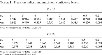
Precision indices and maximum confidence levels
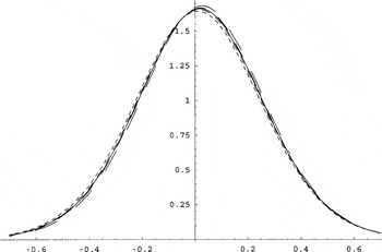
Marginal and conditional densities: OLS estimator. The solid line indicates the marginal density. The dashed lines represent the conditional densities, with the finest line corresponding to the density conditional on f1 and the coarsest line to the density conditional on f4.
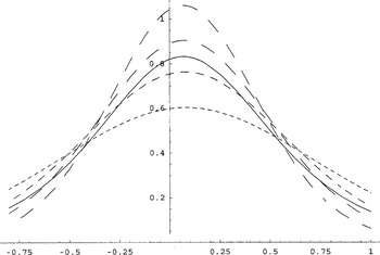
Marginal and conditional densities: TSLS estimator. The solid line indicates the marginal density. The dashed lines represent the conditional densities, with the finest line corresponding to the density conditional on f1 and the coarsest line to the density conditional on f4.
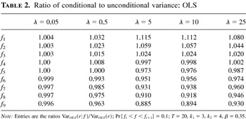
Ratio of conditional to unconditional variance: OLS
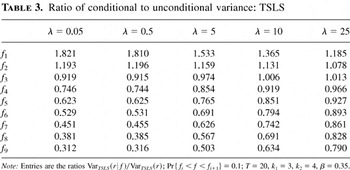
Ratio of conditional to unconditional variance: TSLS
 You have
Access
- 14
- Cited by