


1. Introduction
Variance-optimal hedging was introduced in [Reference Föllmer, Sondermann, Hildenbrand, Mas-Colell and North-Holland12] as a tractable method of hedging contingent claims in incomplete markets (see [Reference Schweizer, Jouini, Cvitanic and Musiela23] for an overview). The main idea of variance-optimal hedging is to find a self-financing trading strategy  ${{\vartheta }^{0}}$
, for a given claim
 $\eta^0$
, which minimizes the (risk-neutral) variance of the residual hedging error at a terminal time
 $T > 0$
. As shown in [Reference Föllmer, Sondermann, Hildenbrand, Mas-Colell and North-Holland12], the solution of this optimization problem is given by the so-called Galtchouk–Kunita–Watanabe (GKW) decomposition of
 $\eta^0$
with respect to the underlying stock S. We assume that we are working under a risk-neutral probability measure
 ${\mathrm{P}}$
and denote by
 ${\mathrm{E}}$
the expectation with respect to
 ${\mathrm{P}}$
: The stock S is a square-integrable martingale with respect to
 ${\mathrm{P}}$
. Then, the GKW decomposition of
 ${\eta}^0$
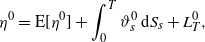
with respect to S takes the form
 \[
\eta^0= {\mathrm{E}}[\eta^0] + \int_0^T\vartheta_s^0{\,\mathrm{d}} S_s + L^0_T ,
\]
where  $L^0$
is a square-integrable martingale orthogonal to S. For applications, it is important to have tractable formulas for the variance-optimal strategy
 $\vartheta^0$
and for the expected squared hedging error
 $\varepsilon^2 \,:\!= {\mathrm{E}}[(L_T^0)^2]$
. To this end, several authors have combined variance-optimal hedging with Fourier methods. This idea was first pursued in [Reference Hubalek, Kallsen and Krawczyk15], where in an exponential Lévy market the expected hedging error was explicitly computed for contingent claims with an integrable and invertible Laplace transform. This method has been further investigated in [Reference Kallsen and Pauwels18], where the underlying market model is a stochastic volatility model described by an affine semimartingale.
In this paper we extend the results of [Reference Hubalek, Kallsen and Krawczyk15,Reference Kallsen and Pauwels18] in two directions: First, we consider a very general setting of semimartingale factor models that is not limited to processes with independent increments or with affine structure. Second, in addition to classic variance-optimal hedging, we also consider the variance-optimal semi-static hedging problem, i.e. we combine dynamic trading in the underlying S with static (i.e. buy-and-hold) positions in a finite number of given contingent claims  ${\pmb{\eta}}\,:\!=({\eta}^1, \dots, {\eta}^d)^{\top}$
, e.g. European puts and calls. Semi-static hedging strategies have been considered for the hedging of barrier options (see [Reference Carr6]), in model-free hedging approaches based on martingale optimal transport (see [Reference Bayraktar and Zhou3,Reference Beiglböck, Henry-Labordère and Penkner4]), and for the semi-static replication of variance swaps by Neuberger’s formula (see [Reference Neuberger21]).
As shown in [Reference Di Tella, Haubold and Keller-Ressel9] and summarized in Section 2 below, the semi-static hedging problem can be solved under a variance-optimality criterion when the covariances  $\varepsilon_{ij} \,:\!= {\mathrm{Cov}}[L_T^i, L_T^{\kern1ptj}]$
of the residuals in the GKW decompositions of all supplementary claims
 $\eta$
are also known. This leads to a natural extension of the questions investigated in [Reference Hubalek, Kallsen and Krawczyk15,Reference Kallsen and Pauwels18]: If the model for S allows for explicit calculation of the moment-generating function of
 $X_T = \log S_T$
(such as Lévy models, the Heston model, or the 3/2 model), and each of the supplementary claims
 $\eta^1, \dotsc, \eta^d$
has a Fourier representation (such as European puts and calls), how can we compute the quantities
 $\varepsilon_{ij}$
? In our main results, Theorems 3.2, 4.1, 4.2, and 4.3, we provide answers to this question and show that the covariances
 $\varepsilon_{ij}$
and the optimal strategies can be recovered by Fourier-type integrals, extending the results of [Reference Hubalek, Kallsen and Krawczyk15,Reference Kallsen and Pauwels18].
We stress that for classical variance-optimal hedging the relevant quantity is  $A\,:\!={\mathrm{E}}[(L^0_T)^2]$
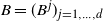
. For the variance-optimal semi-static hedging problem, we additionally need all the covariances
 $B=(B^{\kern1ptj})_{j=1,\ldots,d}$
,
 $B^{\kern1ptj}\,:\!={\mathrm{Cov}}[L_T^0,L^{\kern1ptj}_T]$
and
 $C=(C^{ij})_{i,j=1,\ldots,d}$
,
 $C^{ij}\,:\!=\varepsilon_{ij}$
. Furthermore, we do not assume that
 ${\eta}^0$
has a Fourier representation. Rather, we require that the supplementary claims
 $\pmb{\eta}$
do. The computation of the covariances B and C is completely new, even in the well-studied Heston model.
We now give a brief overview of the companion paper [Reference Di Tella, Haubold and Keller-Ressel9], where we develop numerical results connected with the variance-optimal semi-static hedging problem in the Heston model: We fix a d-dimensional basket of supplementary claims  $\pmb{\eta}$
of European put and call options and set up a variance-optimal semi-static strategy for the variance swap. The quantities A, B, and C, whose analytic expressions are obtained in the present paper, are numerically computed in [Reference Di Tella, Haubold and Keller-Ressel9]. Furthermore, as we shall see below, the variance-optimal semi-static problem can be formulated by two nested minimization problems. The outer minimization problem is interesting because it leads to questions related to optimal subset selection: Given
 $\pmb{\eta}$
, which subset of supplementary claims
 $\pmb{\eta}_k\,:\!=({\eta}^{i_1},\ldots,{\eta}^{i_k})^{\top}$
of cardinality
 $k\leq d$
minimizes the squared hedging error? We call this problem sparse variance-optimal semi-static hedging and we study it in [Reference Di Tella, Haubold and Keller-Ressel9] also comparing different optimal-subset-selection algorithms (e.g. greedy forward selection, Leaps and Bounds, and Lasso).
This paper has the following structure: In Section 2 we collect some notions about stochastic analysis and discuss semi-static variance-optimal strategies. Section 3 is devoted to the study of the GKW decomposition for some square-integrable martingales that play a fundamental role in our setting. In Section 4, we discuss certain problems related to stochastic analysis of processes depending on a parameter and Fourier methods in a general multidimensional factor model. In Section 5 we apply the results of the previous sections to the Heston model (which is an affine model), to the 3/2 model (which is non-affine), and to an exponential Lévy model with jumps.
2. Basic tools and motivation
Let [0,T] be a fixed time interval,  $T>0$
. By
 $({\Omega},{\mathcal{F}},{\mathrm{P}})$
we denote a complete probability space and by
 ${\mathbb{F}}=({\mathcal{F}}_t)_{t\in[0,T]}$
a filtration satisfying the usual conditions. We assume that
 ${\mathcal{F}}_0$
is trivial and that
 ${\mathcal{F}}={\mathcal{F}}_T$
.
We denote by  ${\mathcal{H}}^{\,2}_{\mathbb{C}}$
(resp.
 ${\mathcal{H}}^{\,2}$
) the Hilbert space of càdlàg complex-valued (resp. real-valued)
 ${\mathbb{F}}$
-adapted square-integrable martingales.
If  $X,Y\in{\mathcal{H}}^{\,2}$
, then
 $\left\langle X,Y \right\rangle$
denotes the predictable covariation of X and Y. Notice that X and Y are orthogonal if and only if
 $X_0Y_0=0$
and
 $\left\langle X,Y \right\rangle =0$
.
For  $Z^{\kern1ptj}\,:\!=X^{\kern1ptj}+{\mathrm{i}} Y^{\kern1ptj}\in{\mathcal{H}}^2_{\mathbb{C}}$
,
 $j=1,2$
, we define
 $\left\langle {{Z}^{1}},{{Z}^{2}} \right\rangle :=\left( \left\langle {{X}^{1}},{{X}^{2}} \right\rangle -\left\langle {{Y}^{1}},{{Y}^{2}} \right\rangle \right)+\text{i}\left( \left\langle {{X}^{1}},{{Y}^{2}} \right\rangle +\left\langle {{Y}^{1}},{{X}^{2}} \right\rangle \right).$
For a real- or complex-valued process A of finite variation, we denote by  ${\mathrm{Tv}}(A)$
the total-variation process of A. If H is a (real- or complex-valued) measurable process and A is of finite variation, we denote by
 $\int_0^{\cdot} H_s{\,\mathrm{d}} A_s$
the (Lebesgue–Stieltjes) integral process, if it exists. Recall that
 $\int_0^{\cdot} H_s{\,\mathrm{d}} A_s$
is of finite variation if and only if
 $\int_0^t |H_s({\omega})|{\,\mathrm{d}} {\mathrm{Tv}}(A)_s({\omega})<+\infty$
for every t and
 ${\omega}$
. Furthermore, for such an H and A real-valued, we have
 $
{\mathrm{Tv}}(\int_0^{\cdot} H_s{\,\mathrm{d}} A_s)=\int_0^{\cdot}|H_s|{\,\mathrm{d}}{\mathrm{Tv}}(A)_s.
$
Notice that for  $Z^{\kern1ptj}\,:\!=X^{\kern1ptj}+{\mathrm{i}} Y^{\kern1ptj}\in{\mathcal{H}}^2_{\mathbb{C}}$
,
 $j=1,2$
, by the Kunita–Watanabe inequality for real-valued martingales, we immediately get
 $\text{E}[\text{Tv}{{\left( \left\langle {{Z}^{1}},{{Z}^{2}} \right\rangle \right)}_{t}}]\le 2\text{E}{{[{{\left\langle {{Z}^{1}},{{{\bar{Z}}}^{1}} \right\rangle }_{t}}]}^{1/2}}\text{E}{{[{{\left\langle {{Z}^{2}},{{{\bar{Z}}}^{2}} \right\rangle }_{t}}]}^{1/2}},$
where, for  $Z\in{\mathcal{H}}^2_{\mathbb{C}}$
, we denote by
 $\overline Z\in{\mathcal{H}}^2_{\mathbb{C}}$
the complex conjugate of Z.
For  $X\in{\mathcal{H}}_{\mathbb{C}}^{\,2}$
, we introduce
 $L_{\mathbb{C}}^{2}(X):=\{\vartheta \,\text{predictable}\,\text{and}\,\text{complex-valued}:\text{E}[\int_{0}^{T}{|}{{\vartheta }_{s}}{{|}^{2}}\text{d}{{\left\langle X,\bar{X} \right\rangle }_{s}}]<+\infty \},$
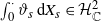
the space of complex-valued integrands for X. For  $\vartheta\in{\mathrm{L}}_{\mathbb{C}}^2(X)$
,
 $\int_0^{\cdot}\vartheta_s{\,\mathrm{d}} X_s\in{\mathcal{H}}^2_{\mathbb{C}}$
denotes the stochastic integral process of
 $\vartheta$
with respect to X. By
 $L^2(X)$
we denote the subspace of
 $L_{\mathbb{C}}^2(X)$
consisting of real-valued elements.
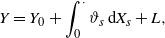
We conclude by recalling the GKW decomposition: Let  $X,Y\in{\mathcal{H}}^2_{\mathbb{C}}$
. Then there exist a unique
 $\vartheta\in L^2_{\mathbb{C}}(X)$
and a unique
 $L\in{\mathcal{H}}^2_{{\mathbb{C}}}$
,
 $L_0=0$
, such that
 $\left\langle X,\bar{L} \right\rangle =0$
(and hence
 $\left\langle L,\bar{X} \right\rangle =0$
), and the decomposition, called the GKW decomposition of Y with respect to X,
 \[
Y=Y_0+\int_0^{\cdot}\vartheta_s{\,\mathrm{d}} X_s+L,
\]
holds. Notice that  $\vartheta =\text{d}\left\langle Y,\bar{X} \right\rangle /\text{d}\left\langle X,\bar{X} \right\rangle$
. We call the orthogonal component Lthe residual in the GKW decomposition of Y with respect to X. For brevity we say that
 $(\vartheta, L)$
is the GKW decomposition of Y with respect to X. Identifying a complex-valued square-integrable and
 ${\mathcal{F}}_T$
-measurable random variable y with the unique (up to indistinguishability) càdlàg martingale
 $Y\in{\mathcal{H}}^2_{\mathbb{C}}$
satisfying
 $Y_t={\mathrm{E}}[y \mid {\mathcal{F}}_t]$
a.s.,
 $t\in[0,T]$
, we also speak of the GKW decomposition of y with respect to X.
2.1. Semi-static variance-optimal hedging
Let  $S\in{\mathcal{H}}^2$
be strictly positive and assume that S models the price process of some stock. This is a crucial assumption on the probability measure
 ${\mathrm{P}}$
: We require that
 ${\mathrm{P}}$
is already an equivalent martingale measure and we do not consider the problem under the historical measure, say
 ${\mathrm{Q}}$
, with respect to which S is, in general, a non-negative semimartingale. This latter case has been considered, e.g., in [Reference Schweizer22]. See also [Reference Schweizer, Jouini, Cvitanic and Musiela23] and the references therein.
A fixed basket of contingent claims  ${\pmb{\eta}}\,:\!=({\eta}^1, \dots, {\eta}^d)^{\top}$
,
 ${\eta}^{\kern1ptj}\in L^2({\mathrm{P}})$
,
 $j=1,\ldots,d$
, is given. We stress that we regard
 ${\mathbb{R}}^d$
as a space of column vectors.
Definition 2.1. (i) A semi-static strategy is a pair  $\left( \vartheta ,v \right)\in {{L}^{2}}\left( S \right)\times {{\mathbb{R}}^{d}}$
. A semi-static strategy is called dynamic if
 $\pmb v=0$
; it is called static if
 $\vartheta=0$
.
(ii) A semi-static variance-optimal hedging strategy for the square-integrable contingent claim  ${\eta}^0$
is a solution of the semi-static variance-optimal hedging problem given by
 \begin{equation}
{{\varepsilon }^{2}}=\overset{\min }{\mathop{_{v\in {{\mathbb{R}}^{d}},\vartheta \in {{\text{L}}^{2}}(S),c\in \mathbb{R}}}}\,\text{E}[{{(c-\text{E}[{{v}^{\top }}\eta ]+\int_{0}^{T}{{{\vartheta }_{s}}}\text{d}{{S}_{s}}-({{\eta }^{0}}-{{v}^{\top }}\text{ }\eta ))}^{2}}].
\label{eqn1}
\end{equation}
In other words, a semi-static strategy is a strategy which, beyond the dynamic (i.e. continuously rebalanced) position in S, also allows a static (i.e. buy-and-hold) position in the fixed basket  $\pmb{\eta}=({\eta}^1, \dots, {\eta}^d)^{\top}$
of contingent claims.
Clearly, (2.1) is a generalization of the classic variance-optimal hedging problem (see, e.g., [Reference Föllmer, Sondermann, Hildenbrand, Mas-Colell and North-Holland12] or [Reference Schweizer, Jouini, Cvitanic and Musiela23]), and semi-static variance-optimal strategies typically allow for a reduction of the quadratic hedging error in comparison with classic variance-optimal strategies.
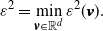
Following [Reference Di Tella, Haubold and Keller-Ressel9], the semi-static hedging problem can be split into an inner and an outer optimization problem. That is, it can be written as an inner problem,
 \begin{equation}
{{\varepsilon }^{2}}(v)=\overset{\min }{\mathop{_{\vartheta \in {{L}^{2}}(S),c\in \mathbb{R}}}}\,\text{E}[{{(c-\text{E}[{{v}^{\top }}\eta ]+\int\limits_{0}^{T}{{{\vartheta }_{s}}}\text{d}{{S}_{s}}-({{\eta }^{0}}-{{v}^{\top }}\text{ }\eta ))}^{2}}],
\label{eqn2}
\end{equation}
and an outer problem,
 \begin{equation}
\displaystyle\varepsilon^2 = \min_{\pmb v \in {\mathbb{R}}^d}{\varepsilon^2(\pmb v)}.
\label{eqn3}
\end{equation}
Now let  $(\vartheta^{\kern1ptj},L^{\kern1ptj})$
be the GKW decomposition of
 ${\eta}^{\kern1ptj}$
with respect to S,
 $j=0,\ldots,d$
. Since (2.2) is a classic variance-optimal hedging problem, the optimal solution
 $(\vartheta^{\pmb v,\ast},c^{\ast})$
is given by the integrand
 $\vartheta^{\pmb v,\ast}\in L^2(S)$
appearing in the GKW decomposition of
 ${\eta}^0-\pmb v^{\top}\pmb{\eta}$
with respect to S, that is,
 $\vartheta^{\pmb v,\ast}=\vartheta^0-\sum_{j=1}^dv_j\vartheta^{\kern1ptj}$
, and
 $c^{\ast}={\mathrm{E}}[{\eta}^0]$
.
The outer problem (2.3) is a finite-dimensional quadratic optimization problem, since  $\varepsilon^2(\pmb v)$
is of the form
 $${{\varepsilon }^{2}}(v)=A-2\text{ }{{v}^{\top }}B+\text{ }{{v}^{\top }}Cv,$$
where the coefficients A, B, and C are given by
 \begin{align}
A:=\text{E}[{{\left\langle {{L}^{0}},{{L}^{0}} \right\rangle }_{T}}],\ \ {{B}^{j}}:=\text{E}[{{\left\langle {{L}^{0}},{{L}^{j}} \right\rangle }_{T}}],\ \ {{C}^{ij}}:=\text{E}[{{\left\langle {{L}^{i}},{{L}^{j}} \right\rangle }_{T}}],\quad i,j=1,\ldots ,d.
\label{eqn4}
\end{align}
If C is invertible, then the optimal strategy  $(\vartheta^{\ast},\pmb v^{\ast}, c^{\ast})$
for the semi-static variance-optimal hedging problem (2.1) is given by
 \[\pmb v^* = C^{-1} B, \quad \vartheta^{\ast} = \vartheta^0 - \sum_{j=1}^dv_j^{\ast} \vartheta^{\kern1ptj},\quad c^{\ast}={\mathrm{E}}[{\eta}^0].\]
Hence, to solve the semi-static variance-optimal hedging problem, it is necessary to compute the predictable covariations of the residuals in the GKW decomposition of  ${\eta}^{\kern1ptj}$
with respect to S,
 $j=1,\ldots,d$
, and then their expectation. This extends beyond the classic variance-optimal hedging problem, where it is enough to determine A in order to compute the squared hedging error and the optimal strategy.
3. The GKW decomposition in factor models
Let  $S,Y^i\in{\mathcal{H}}^2_\mathrm{loc}$
and let
 $(\vartheta^i, L^i)$
be the GKW decomposition of
 $Y^i$
with respect to S,
 $i=1,2$
. In this section we compute
 $\vartheta^i$
,
 $i=1,2$
, and the predictable covariation
 $\left\langle {{L}^{1}},{{L}^{2}} \right\rangle$
. This is motivated by Section 2, where we have seen that these predictable covariations are needed to compute the solution of (2.1).
3.1. Martingale representation
We consider a quasi-left continuous locally square-integrable semimartingale  $X=(X^1,\ldots,X^n)^{\top}$
with state space
 $(E,{\mathcal{E}})\,:\!=({\mathbb{R}}^ n,{\mathcal{B}}({\mathbb{R}}^n))$
(see [16, Definition II.2.27]). Then, for
 $j=1,\ldots,n$
, the unidimensional semimartingale
 $X^{\kern1ptj}$
admits the unique decomposition
 \begin{equation}
X^{\kern1ptj}=X^{\kern1ptj}_0+M^{\kern1ptj}+A^{\kern1ptj},
\label{eqn5}
\end{equation}
where  $A^{\kern1ptj}$
is a continuous adapted process of finite variation and
 $M^{\kern1ptj}\in{\mathcal{H}}^2_\mathrm{loc}$
is quasi-left continuous,
 $j=1,\ldots,n$
. We denote by
 $X^{j,c}$
the continuous martingale part of
 $X^{\kern1ptj}$
. Let
 $Y\in{\mathcal{H}}^2_{\mathrm{loc}}$
be of the form
 \begin{equation}
Y_t = f(t,X_t),\quad f\in C^{1,2}({\mathbb{R}}_+\times{\mathbb{R}}^n).
\label{eqn6}
\end{equation}
We are going to show that Y has the representation property relative to X (see [16, Definition III.4.22]) and also obtain an explicit form of the integrand. To tackle the problem, we pursue the following classical idea: We consider  $Y\in{\mathcal{H}}^2_\mathrm{loc}$
, which is given by a function
 $f\in C^{1,2}({\mathbb{R}}_+\times{\mathbb{R}}^n)$
of time and X. Then, applying Itô’s formula, we show that Y has the representation property relative to X.
Such kinds of martingale representation results have already been considered in the literature, especially for pricing of European options: In [8, Section 3] this result has been shown in a Brownian context, and in [11, Section 3] for the homogeneous Poisson case. In [5, Section 2] the case of a continuous semimartingale is considered. We add a new element to this picture by considering locally square-integrable quasi-left continuous semimartingales.
We denote by  $\mu$
be the jump measure of X, by
 $\nu$
its predictable compensator, and we put
 $\overline\mu\,:\!=\mu-\nu$
. By
 $\mathcal{G}_{\text{loc}}^{2}\left(\mu\right)$
we denote the space of predictable integrands W on
 $[0,T]\times{\Omega}\times E$
such that the stochastic integral
 $Z=\int_0^{\cdot}\int_E W(s,x)\overline\mu({\mathrm{d}} s,{\mathrm{d}} x)$
is the unique (up to indistinguishability) purely discontinuous element of
 ${\mathcal{H}}^2_\mathrm{loc}$
such that
 $Z_0=0$
and
 $\Delta Z=W(\cdot,\Delta X)1_{\{\Delta X\neq0\}}$
. For details, see [16, Section II.1d].
For  $Y\in{\mathcal{H}}^2_\mathrm{loc}$
, we denote by
 $Y^d\in{\mathcal{H}}^2_\mathrm{loc}$
the purely discontinuous part of Y (see [16, Theorem I.4.18]).
Theorem 3.1. Let  $X=(X^1,\ldots,X^n)^{\top}$
be a quasi-left continuous locally square-integrable semimartingale such that
 $X^{\kern1ptj}$
has the canonical decomposition as in (3.1),
 $j=1,\ldots,n$
. Let
 $\mu$
be the jump measure of X,
 $\nu$
the predictable compensator of
 $\mu$
, and
 $\overline\mu\,:\!=\mu-\nu$
. Let
 $Y=(Y_t)_{t\in[0,T]}\in{\mathcal{H}}^2_\mathrm{loc}$
be as in (3.2). Then, denoting by
 $\partial_{\cdot}$
the partial derivative,
 \begin{equation}
Y=Y_0+\sum_{j=1}^n \int_0^{\cdot} \partial_{x_j}\,f(s,X_{s-}){\,\mathrm{d}} X^{j,c}_s+\int_0^{\cdot}\int_E [\:f(s,x+X_{s-})-f(s,X_{s-})]\,\overline\mu({\mathrm{d}} s,{\mathrm{d}} x).
\label{eqn7}
\end{equation}
Proof. By Itô’s formula and (3.1), we deduce that
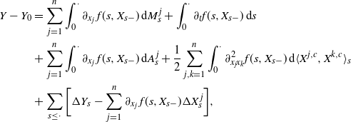 \begin{equation}
\begin{split}
Y-{{Y}_{0}}&=\sum\limits_{j=1}^{n}{\int_{0}^{\cdot }{{{\partial }_{{{x}_{j}}}}}}f(s,{{X}_{s-}})\text{d}M_{s}^{j}+\int_{0}^{\cdot }{{{\partial }_{t}}}f(s,{{X}_{s-}})\text{d}s\\
&+\sum\limits_{j=1}^{n}{\int_{0}^{\cdot }{{{\partial }_{{{x}_{j}}}}}}f(s,{{X}_{s-}})\text{d}A_{s}^{j}+\frac{1}{2}\sum\limits_{j,k=1}^{n}{\int_{0}^{\cdot }{\partial _{{{x}_{j}}{{x}_{k}}}^{2}}}f(s,{{X}_{s-}})\text{d}{{\left\langle {{X}^{j,c}}{{X}^{k,c}} \right\rangle }_{s}}\\
&+\sum\limits_{s\le \cdot }{[}\Delta {{Y}_{s}}-\sum\limits_{j=1}^{n}{{{\partial }_{{{x}_{j}}}}}f(s,{{X}_{s-}})\Delta X_{s}^{j}],
\end{split}
\label{eqn8}
\end{equation}
where  $\partial^2_{\cdot\cdot}$
denotes the second partial derivative. We denote by N the first term and by G the sum of the second, the third, and the fourth terms on the right-hand side of (3.4). Finally, we set
 $
U(t,x)\,:\!=f(t,x+X_{t-})-f(t,X_{t-})-\sum_{j=1}^n\partial_{x_j}\, f(t,X_{t-}) x_j
$
. The process U belongs to
 ${\mathcal{G}}^2_\mathrm{loc}(\mu)$
. Indeed, because of (3.4) and the continuity of G,
 $\Delta (Y-N)=U(\cdot,\Delta X)$
. Hence,
 $\sum_{s\leq\cdot}U_s^2\leq[Y-N,Y-N]$
and
 $[Y-N,Y-N]$
is locally integrable because
 $Y-N\in{\mathcal{H}}^2_\mathrm{loc}$
. Thus,
 $Z\,:\!=\int_0^{\cdot}\int_E U(s,x)\,\overline\mu({\mathrm{d}} s,{\mathrm{d}} x)\in{\mathcal{H}}^2_\mathrm{loc}$
. Furthermore, because of (3.4), we have
 $J\,:\!=\sum_{s\leq \cdot}U(s,\Delta X_s)+G\in{\mathcal{H}}^2_\mathrm{loc}$
and J is of finite variation. Hence, J is a purely discontinuous local martingale and
 $\Delta Z=\Delta J$
. From [16, Corollary I.4.19], Z and J are indistinguishable and (3.4) becomes
 \[
Y=Y_0+\sum_{j=1}^n\int_0^{\cdot}\partial_{x_j}\, f(s,X_{s-}){\,\mathrm{d}} M^{\kern1ptj}_s+\int_0^{\cdot}\int_E U(s,x)\,\overline\mu({\mathrm{d}} s,{\mathrm{d}} x).
\]
Since, for  $j=1,\ldots,n$
, we have
 $M^{\kern1ptj}=X^{ j,c}+(M^{j})^d$
and
 ${{({{M}^{j}})}^{d}}={{x}_{j}}*\bar{\mu}$
, we get the desired result by [16, Proposition II.1.30 (b)] and by linearity.
We now assume that  $S\in{\mathcal{H}}^2_\mathrm{loc}$
is of the form
 $S={\mathrm{e}}^{X^1}$
. Denoting by
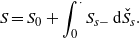
 ${\skew3\check S}$
the stochastic logarithm of S, we have
 \begin{equation}
S=S_0+\int_0^{\cdot} S_{s-}{\,\mathrm{d}} {\skew3\check S}_s.
\label{eqn9}
\end{equation}
Applying Theorem 3.1 to  $f(t,x)={\mathrm{e}}^{x_1}$
yields
 \begin{equation}
{\skew3\check S}\,:\!={\skew3\check S}_0+(X^{1, c}+{\skew3\check S}^d),\quad{\skew3\check S}^d\,:\!=\int_0^{\cdot}\int_E({\mathrm{e}}^{x_1}-1)\,\overline\mu({\mathrm{d}} s,{\mathrm{d}} x)
\label{eqn10}
\end{equation}
and, since  $x\mapsto({\mathrm{e}}^{x_1}-1)\in{\mathcal{G}}^2_\mathrm{loc}(\mu)$
, we have
 ${\skew3\check S} \in{\mathcal{H}}^2_\mathrm{loc}$
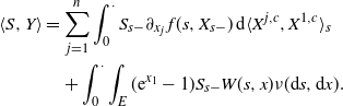
. If Y is as in (3.2), then Theorem 3.1, (3.5), (3.6), and [16, Theorem II.1.33(a)] imply that
 \begin{align}
\left\langle S,Y \right\rangle &=\sum\limits_{j=1}^{n}{\int_{0}^{\cdot }{{{S}_{s-}}}}{{\partial }_{{{x}_{j}}}}f(s,{{X}_{s-}})\text{d}{{\left\langle {{X}^{j,c}},{{X}^{1,c}} \right\rangle }_{s}}\\
&+\int_{0}^{\cdot }{\int_{E}{({{\text{e}}^{{{x}_{1}}}}-1)}}{{S}_{s-}}W(s,x)\nu (\text{d}s,\text{d}x).
\label{eqn11}\end{align}
Theorem 3.2. Let  $X=(X^1,\ldots,X^2)^{\top}$
be a quasi-left continuous locally square-integrable semimartingale such that
 $X^{\kern1ptj}$
has the canonical decomposition as in (3.1),
 $j=1,\ldots,d$
. Let
 $\mu$
be the jump measure of X,
 $\nu$
the predictable compensator of
 $\mu$
, and
 $\overline\mu\,:\!=\mu-\nu$
. Let
 $S={\mathrm{e}}^{X^1}\in{\mathcal{H}}^2_\mathrm{loc}$
. Let
 $Y^i\in{\mathcal{H}}^2_\mathrm{loc}$
be such that
 $Y^i_t=f^i(t,X_t)$
as in (3.2) and put
 $Y^{i,d}\,:\!=(Y^i)^d$
,
 $i=1,2$
. Then the GKW decomposition
 $(\vartheta^i, L^i)$
of
 $Y^i$
with respect to S is given by
 $L^i=Y^i-Y^i_0-\int_0^{\cdot}\vartheta^i_s{\,\mathrm{d}} S_s$
and, for all
 $t\in[0,T]$
,
 \begin{equation}
\vartheta _{t}^{i}=\frac{1}{{{S}_{t-}}}(\sum\limits_{j=1}^{n}{{{\partial }_{{{x}_{j}}}}}{{f}^{i}}(t,{{X}_{t-}})\frac{\text{d}{{\left\langle {{X}^{1,c}},{{X}^{j,c}} \right\rangle }_{t}}}{\text{d}{{\left\langle \overset{}{\skew3\check S}\,,\overset{}{\skew3\check S}\, \right\rangle }_{t}}}+\frac{\text{d}{{\left\langle {{\overset{}{\skew3\check S}\,}^{d}},{{Y}^{i,d}} \right\rangle }_{t}}}{\text{d}{{\left\langle \overset{}{\skew3\check S}\,,\overset{}{\skew3\check S}\, \right\rangle }_{t}}}),\quad i=1,2.
\label{eqn12}
\end{equation}
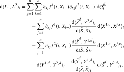
Moreover, setting
 \[{{Q}^{jk}}:=\left\langle {{X}^{j,c}},{{X}^{k,c}} \right\rangle -\int_{0}^{\cdot }{\frac{d\left\langle {{X}^{1,c}},{{X}^{j,c}} \right\rangle s}{d{{\left\langle \overset{{\skew3\check S}}\,,\overset{{\skew3\check S}}\, \right\rangle }_{s}}}}\text{d}{{\left\langle {{X}^{1,c}},{{X}^{k,c}} \right\rangle }_{s,}}\]
we have
 \begin{equation}
\begin{split}
\text{d }{{\left\langle {{L}^{1}},{{L}^{2}} \right\rangle }_{t}}&=\sum\limits_{j=1}^{n}{\sum\limits_{k=1}^{n}{{{\partial }_{{{x}_{j}}}}}}{{f}^{1}}(t,{{X}_{t-}}){{\partial }_{{{x}_{k}}}}{{f}^{2}}(t,{{X}_{t-}})\text{d}Q_{t}^{jk}\\
&-\sum\limits_{j=1}^{n}{{{\partial }_{{{x}_{j}}}}}{{f}^{1}}(t,{{X}_{t-}})\frac{{{\left\langle \text{d}{{\overset{}{\skew3\check S}\,}^{d}},{{Y}^{2,d}} \right\rangle }_{t}}}{\text{d}{{\left\langle \overset{}{\skew3\check S}\,,\overset{}{\skew3\check S}\, \right\rangle }_{t}}}\text{d}{{\left\langle {{X}^{1,c}},{{X}^{j,c}} \right\rangle }_{t}}\\
&-\sum\limits_{j=1}^{n}{{{\partial }_{{{x}_{j}}}}}{{f}^{2}}(t,{{X}_{t-}})\frac{\text{d}{{\left\langle {{\overset{}{\skew3\check S}\,}^{d}}{{Y}^{1,d}} \right\rangle }_{t}}}{\text{d}{{\left\langle \overset{}{\skew3\check S}\,,\overset{}{\skew3\check S}\, \right\rangle }_{t}}}\text{d}{{\left\langle {{X}^{1,c}},{{X}^{j,c}} \right\rangle }_{t}}\\
&+\text{d}{{\left\langle {{Y}^{1,d}},{{Y}^{2,d}} \right\rangle }_{t}}-\frac{\text{d}{{\left\langle {{\overset{}{\skew3\check S}\,}^{d}},{{Y}^{1,d}} \right\rangle }_{t}}}{\text{d}{{\left\langle \overset{}{\skew3\check S}\,,\overset{}{\skew3\check S}\, \right\rangle }_{t}}}\text{d}{{\left\langle {{\overset{}{\skew3\check S}\,}^{d}}{{Y}^{2,d}} \right\rangle }_{t,}}
\end{split}
\label{eqn13}
\end{equation}
where, denoting  $W^i(t,x)\,:\!=f^i(t,x+X_{t-})-f^i(t,X_{t-})$
,
 $i=1,2$
, we have
 \begin{eqnarray}
\left\langle \overset{}{\skew3\check S}\,,\overset{}{\skew3\check S}\, \right\rangle =\left\langle {{X}^{1,c}},{{X}^{1,c}} \right\rangle +\int_{0}^{\cdot }{\int_{E}{{{({{\text{e}}^{{{x}_{1}}}}-1)}^{2}}}}\nu (\text{d}s,\text{d}x),
\label{eqn14}
\end{eqnarray}
 \begin{eqnarray}
\left\langle {{\overset{}{\skew3\check S}\,}^{d}},{{\overset{}{\skew3\check S}\,}^{d}} \right\rangle =\int_{0}^{\cdot }{\int_{E}{{{({{\text{e}}^{{{x}_{1}}}}-1)}^{2}}}}\nu (\text{d}s,\text{d}x),
\label{eqn15}\end{eqnarray}
 \begin{eqnarray}
\left\langle {{\overset{}{\skew3\check S}\,}^{d}},{{Y}^{i,d}} \right\rangle =\int_{0}^{\cdot }{\int_{E}{({{\text{e}}^{{{x}_{1}}}}-1)}}{{W}^{i}}(s,x)\nu (\text{d}s,\text{d}x),
\label{eqn16}\end{eqnarray}
 \begin{eqnarray}
\left\langle {{Y}^{1,d}},{{Y}^{2,d}} \right\rangle =\int_{0}^{\cdot }{\int_{E}{{{W}^{1}}}}(s,x){{W}^{2}}(s,x)\nu (\text{d}s,\text{d}x).
\label{eqn17}\end{eqnarray}
Proof. Clearly, (3.10) and (3.11) follow from (3.6); (3.12) follows from (3.7); and (3.13) is a consequence of Theorem 3.1. Formula (3.8) follows by Theorem 3.1 and (3.6), because of  ${{\vartheta }^{i}}=\text{d}\left\langle S,{{Y}^{i}} \right\rangle /\text{d}\left\langle S,S \right\rangle$
,
 $i=1,2$
, and of
 $\left\langle S,S \right\rangle =S_{-}^{2}\cdot \left\langle \overset{}{\skew3\check S}\,,\overset{}{\skew3\check S}\, \right\rangle$
. To show (3.9) we consider the identity
 $
\left\langle {{L}^{1}},{{L}^{2}} \right\rangle =\left\langle {{Y}^{1}},{{Y}^{2}} \right\rangle -\int_{0}^{\cdot }{\vartheta _{s}^{1}}\vartheta _{s}^{2}\text{d}{{\left\langle S,S \right\rangle }_{s}}
$
, compute
 $\left\langle {{Y}^{1}},{{Y}^{2}} \right\rangle$
from Theorem 3.1, and use (3.8) and (3.10). The proof is complete.
Let  $(B,C,\nu)$
denote the semimartingale characteristics of X (cf. [16, II.§2a]) relative to the truncation function
 $h=(h^1,\ldots,h^n)^{\top}$
, where
 $h^{\kern1ptj}(x)=x_j1_{\{|x_j|\leq1\}}$
,
 $j=1,\ldots,n$
. Let us assume that
 $(B,C,\nu)$
are absolutely continuous with respect to the Lebesgue measure on [0,T] (which we denote by
 ${\mathrm{Leb.}}$
): By (b, c, F) we denote the predictable differential characteristics of X. We stress that
 $F_t({\omega},{\,\mathrm{d}} x)$
is a measure on
 $({\mathbb{R}}^n,{\mathcal{B}}({\mathbb{R}}^n))$
and
 $C^{\,jk}=\int_0^{\cdot} c^{\,jk}_s{\,\mathrm{d}} s$
,
 $j,k=1,\ldots,n$
. We get the following corollary to Theorem 3.2.
Corollary 3.1. Let (b, c, F) be the predictable differential characteristics of X.
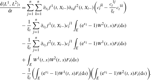
(i) Setting  $\xi_t\,:\!=c_t^{11}+\int_E({\mathrm{e}}^{x_1}-1)^2F_t({\mathrm{d}} x)$
,
 $t\in[0,T]$
, we get,
 ${\mathrm{Leb.}}$
-a.e.,
 \begin{equation}
\vartheta_t^i=\frac{1}{S_{t-}\xi_t}\bigg(\sum_{j=1}^n\partial_{x_j}\,f^i(t,X_{t-})c^{1j}_t+\int_E({\mathrm{e}}^{x_1}-1)W^i(t,x)F_t({\mathrm{d}} x)\bigg), \quad i=1,2,
\label{eqn18}
\end{equation}
and (3.9) becomes
 \begin{equation}
\begin{split}
\frac{\text{d }{{\left\langle {{L}^{1}},{{L}^{2}} \right\rangle }_{t}}}{\text{d}t}&
=\sum_{j=1}^n\sum_{k=1}^n\partial_{x_j}\,f^1(t,X_{t-})\partial_{x_k}f^2(t,X_{t-})\bigg(c^{\,jk}_t-\frac{c^{\,1j}_t}{\xi_t}c^{\,1k}_t\bigg)
\\&-
\frac1{\xi_t}\sum_{j=1}^n\partial_{x_j}\,f^1(t,X_{t-})c^{\,j1}_t\int_E({\mathrm{e}}^{x_1}-1)W^2(t,x)F_t({\mathrm{d}} x)
\\&-
\frac1{\xi_t}\sum_{j=1}^n\partial_{x_j}\,f^2(t,X_{t-})c^{\,j1}_t\int_E({\mathrm{e}}^{x_1}-1)W^1(t,x)F_t({\mathrm{d}} x)
\\&+
\int_EW^1(t,x)W^2(t,x)F_t({\mathrm{d}} x)
\\&-\frac1{\xi_t}\bigg(\!\int_E({\mathrm{e}}^{x_1}-1)W^1(t,x)F_t({\mathrm{d}} x)\bigg)\!\bigg(\!\int_E({\mathrm{e}}^{x_1}-1)W^2(t,x)F_t({\mathrm{d}} x)\bigg).
\end{split}
\label{eqn19}
\end{equation}
(ii) If, furthermore, X is continuous, then
 \begin{equation*}\label{eq:var.opt.str.abs.con.con}
\vartheta_t^i=\frac{1}{S_{t}c^{11}_t}\sum_{j=1}^n\partial_{x_j}\,f^i(t,X_{t})c^{1j}_t,\quad i=1,2,
\end{equation*}
and
 \begin{equation}
\frac{\text{d}{{\left\langle {{L}^{1}},{{L}^{2}} \right\rangle }_{t}}}{\text{d}t}
=\sum_{j=2}^n\sum_{k=2}^n\partial_{x_j}\,f^1(t,X_{t})\partial_{x_k}f^2(t,X_{t})\bigg(c^{\,jk}_t-\frac{c^{\,1j}_t}{c^{\,11}_t}c^{\,1k}_t\bigg).
\label{eqn20}
\end{equation}
We remark that in the case of absolutely continuous semimartingale characteristics as described in Corollary 3.1, by (3.5) and (3.6) we get  $\left\langle S,S \right\rangle =\int_{0}^{\cdot }{S_{s-}^{2}}{{\xi }_{s}}\text{d}s$
.
4. Models with Fourier representation
In this section we combine variance-optimal semi-static hedging with Fourier methods. We do not assume a special stochastic volatility model (in [Reference Kallsen and Pauwels18] affine models were considered). This requires some technical considerations about stochastic processes depending on a parameter. A seminal paper about this topic is [Reference Stricker and Yor24].
4.1. Complex-valued processes depending on a parameter
We denote by  ${\mathcal{S}}\subseteq{\mathbb{C}}^n$
the space of parameters and consider the Borel
 ${\sigma}$
-algebra
 ${\mathcal{B}}({\mathcal{S}})$
. On
 $({\mathcal{S}},{\mathcal{B}}({\mathcal{S}}))$
a finite complex-valued measure
 ${\zeta}$
is given. We recall that with
 ${\zeta}$
we can associate the positive measure
 $|{\zeta}|$
, called the total variation of
 ${\zeta}$
. Moreover,
 ${\mathrm{d}}{\zeta}=h\,{\mathrm{d}}|{\zeta}|$
, where h is a complex-valued function such that
 $|h|=1$
. So,
 $L^1({\zeta})=L^1(|{\zeta}|)$
.
We set  $\widetilde{\Omega}\,:\!={\Omega}\times[0,T]\times{\mathcal{S}}$
. If
 ${\mathcal{O}}$
(resp.
 ${\mathcal{P}}$
) is the optional (resp. predictable)
 ${\sigma}$
-algebra, then we set
 $\widetilde {\mathcal{O}}\,:\!={\mathcal{O}}\otimes{\mathcal{B}}({\mathcal{S}})$
(resp.
 $\widetilde {\mathcal{P}}\,:\!={\mathcal{P}}\otimes{\mathcal{B}}({\mathcal{S}})$
).
We denote by  $\skew3\widetilde U$
a function on
 $\widetilde{\Omega}$
and we say that
 $(t,\omega ,z)\mapsto \text{ }\widetilde{U}{{(\omega ,z)}_{t}}$
is an optional (resp. a predictable) function if it is
 $\widetilde{\mathcal{O}}$
-measurable (
 $\widetilde{\mathcal{P}}$
-measurable). Sometimes, to specify the
 ${\sigma}$
-algebra
 ${\mathcal{B}}({\mathcal{S}})$
, we say that
 $\skew3\widetilde U$
is an optional (resp. predictable) function with respect to
 ${\mathcal{S}}$
. We denote by
 ${\mathrm{Leb.}}$
the Lebesgue measure on [0,T].
Convention.
We assume that all quantities explicitly depending on  $z\in{\mathcal{S}}$
are complex-valued.
Lemma 4.1. Let  $\skew3\widetilde U$
be an optional function such that
 $\skew3\widetilde U(z)$
is a complex-valued square-integrable martingale (non-necessarily càdlàg) for every
 $z\in{\mathcal{S}}$
, and furthermore assume that
 $\sup_{z\in{\mathcal{S}}}{\mathrm{E}}[|\skew3\widetilde U(z)_t|^2]<+\infty$
, for every
 $t\in[0,T]$
. Then the process
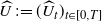 $\skew3\widehat U\,:\!=(\skew3\widehat U_t)_{t\in[0,T]}$
,
 $\skew3\widehat U_t\,:\!=\int_{\mathcal{S}} \skew3\widetilde U(z)_t{\zeta}({\mathrm{d}} z)$
, is a (non-necessarily càdlàg) complex-valued square-integrable martingale. If, additionally,
 $t\mapsto \skew3\widetilde U({\omega},z)_t$
is càdlàg, then
 $\skew3\widehat U$
is a.s. càdlàg.
Proof. We observe that Tonelli’s theorem yields
 \[
{\mathrm{E}}\left[\!\int_{\mathcal{S}}|\skew3\widetilde U(z)_t|^2|{\zeta}|({\mathrm{d}} z)\right]\leq |{\zeta}|({\mathcal{S}})\sup_{z\in{\mathcal{S}}} {\mathrm{E}}[|{ \skew3\widetilde U(z)_t}|^2]<+\infty,\quad t\in[0,T].
\]
So,  $z\mapsto \skew3\widetilde U({\omega},z)_t\in L^2({\zeta})$
a.s.,
 $t\in[0,T]$
, and
 $\skew3\widehat U$
is adapted,
 $(\omega ,z)\mapsto \widetilde{U}{{(\omega ,z)}_{t}}$
being
 ${\mathcal{F}}_t\otimes{\mathcal{B}}({\mathcal{S}})$
-measurable, for every
 $t\in[0,T]$
. Fubini’s theorem now yields that
 $\skew3\widehat U$
is a complex-valued square-integrable martingale (non-necessarily càdlàg). If
 $t\mapsto \skew3\widetilde U({\omega},z)_t$
is càdlàg, then
 $\left( s,\omega ,z \right)\mapsto {{\sup }_{t\in \left[ 0,s \right]}}|\widetilde{U}{{\left( \omega ,z \right)}_{t}}|$
is optional and Tonelli’s theorem and Doob’s inequality yield
 ${\mathrm{E}}[\!\int_{\mathcal{S}} \sup_{t\in[0,T]}|\skew3\widetilde U(z)_t|^2|{\zeta}|({\mathrm{d}} z)]<+\infty$
. Therefore, we have
 $|\skew3\widetilde U(z)_t|\leq\sup_{t\in[0,T]} |\skew3\widetilde U(z)_t|\in L^2({\zeta})$
a.s. Hence, by dominated convergence,
 $\skew3\widehat U$
is a.s. càdlàg. The proof is complete.
To compute the point brackets of square-integrable martingales with a representation as in Lemma 4.1, we shall use the next proposition.
Proposition 4.1. Let  $\widetilde V$
be a function on
 $\widetilde {\Omega}$
such that
 $\widetilde V(z)\in{\mathcal{H}}^2_{\mathbb{C}}$
, for all
 $z\in{\mathcal{S}}$
, and
 $\sup_{z\in{\mathcal{S}}}{\mathrm{E}}[|\widetilde V(z)_T|^2]<+\infty$
. Let
 $Z\in{\mathcal{H}}^2_{\mathbb{C}}$
and let
 $
(t,\omega ,z)\mapsto {{\left\langle Z,\tilde{V}(z) \right\rangle }_{t}}(\omega )
$
be a predictable function.
(i) Then the function  $
(t,\omega ,z)\mapsto \text{Tv}{{(\left\langle Z,\tilde{V}(z) \right\rangle )}_{t}}(\omega)
$
is predictable and
 \begin{equation}
\text{E}\left[ \int_{\mathcal{S}}{\text{Tv}}{{(\left\langle Z,\tilde{V}(z) \right\rangle )}_{T}}|\zeta |(\text{d}z) \right]<+\infty.
\label{eqn21}
\end{equation}
Moreover, the process  $D=(D_t)_{t\in[0,T]}$
,
 $
{{D}_{t}}:={{\int_{\mathcal{S}}{\left\langle Z,\tilde{V}(z) \right\rangle }}_{t}}\zeta (\text{d}z)
$
, is well defined for all
 $t\in[0,T]$
a.s. Furthermore, D is càdlàg, predictable, of finite variation, and
 $D_0=0$
.
(ii) Let  $\skew3\widetilde U$
be an optional function and
 $\skew3\widetilde U(z)$
be a (non-necessarily càdlàg) version of
 $\widetilde V(z)$
for every
 $z\in{\mathcal{S}}$
. Then
 $\sup_{z\in{\mathcal{S}}}{\mathrm{E}}[|\skew3\widetilde U(z)_t|^2]<+\infty$
,
 $t\in[0,T]$
, and the process
 $\skew3\widehat U=(\skew3\widehat U_t)_{t\in[0,T]}$
,
 $\skew3\widehat U_t\,:\!=\int_{\mathcal{S}}\skew3\widetilde U(z)_t{\zeta}({\mathrm{d}} z)$
, is a complex-valued square-integrable martingale. Let
 $U^{\ast}$
be a càdlàg version of
 $\skew3\widehat U$
. Then
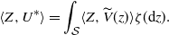 \begin{equation}
\left\langle Z,{{U}^{*}} \right\rangle =\int_{\mathcal{S}}{\left\langle Z\text{,}\tilde{V}(z) \right\rangle }\zeta (\text{d}z).
\label{eqn22}
\end{equation}
(iii) If  $\widetilde K$
is a predictable function such that
 $\int_0^T|\widetilde K({\omega},z)_s|{\,\mathrm{d}} s<+\infty$
,
 $
(\omega ,z)\in \Omega \times \mathcal{S}
$
, and
 ${{\left\langle Z,\tilde{V}(z) \right\rangle }_{t}}(\omega )=\int_{0}^{t}{\tilde{K}{{(\omega ,z)}_{s}}\text{d}s,}$
then  $
(t,\omega ,z)\mapsto {{\left\langle Z,\tilde{V}(z) \right\rangle }_{t}}(\omega )
$
is a predictable function,
 $\widetilde K\in L^1(\widetilde {\mathcal{P}},{\mathrm{P}}\otimes{\mathrm{Leb.}}\otimes{\zeta})$
, and
 \begin{equation}
\left\langle Z,{{U}^{*}} \right\rangle =\int_{\mathcal{S}}{\int_{0}^{\cdot }{\text{ }}}\tilde{K}{{(z)}_{s}}\text{d}s\zeta (\text{d}z)=\int_{0}^{\cdot }{\int_{\mathcal{S}}{\tilde{K}{{(z)}_{s}}\zeta (\text{d}z)\text{d}s}}
\label{eqn23}
\end{equation}
holds. Furthermore,  $\text{E}[\left\langle Z,{{U}^{*}} \right\rangle ]=\int_{0}^{\cdot }{\int_{\mathcal{S}}{\text{E}}}[\tilde{K}{{(z)}_{s}}]\zeta (\text{d}z)\text{d}s$
.
Proof. We first prove (i). The predictability of  $
(t,\omega ,z)\mapsto \text{Tv}{{(\left\langle Z,\tilde{V}(z) \right\rangle )}_{t}}(\omega )
$
follows from the predictability of
 $
(t,\omega ,z)\mapsto {{\left\langle Z,\tilde{V}(z) \right\rangle }_{t}}(\omega )
$
and from
 $
\text{Tv}{{(\left\langle Z,\tilde{V}(z) \right\rangle )}_{t}}=\underset{n\to +\infty }{\mathop{\lim }}\,\sum\limits_{k=1}^{n}{|}{{\left\langle Z,\tilde{V}(z) \right\rangle }_{tk/n}}-{{\left\langle Z,\tilde{V}(z) \right\rangle }_{t(k-1)/n}}|.
$
To prove (4.1), we observe that Tonelli’s theorem, the Kunita–Watanabe inequality, and the relation  $
\text{E}[{{\left\langle X,\bar{X} \right\rangle }_{t}}]\le \text{E}[|{{X}_{t}}{{|}^{2}}]
$
,
 $t\geq0$
, valid for every
 $X\in{\mathcal{H}}^2_{\mathbb{C}}$
(
 $\overline X$
denoting the complex conjugate of X), imply that
 $
\text{E}[\int_{\mathcal{S}}{\text{Tv}}{{(\left\langle Z,\tilde{V}(z) \right\rangle )}_{T}}|\zeta |(\text{d}z)]\le 2\text{E}{{[|{{Z}_{T}}{{|}^{2}}]}^{1/2}}{{(\underset{z\in \mathcal{S}}{\mathop{\sup }}\,\text{E}[|\tilde{V}{{(z)}_{T}}{{|}^{2}}])}^{1/2}}|\zeta |(\mathcal{S})<+\infty.
$
This proves (4.1). From (4.1), since  $\rm su{{p}_{t\in [0,T]}}|{{\left\langle Z,\tilde{V}(z) \right\rangle }_{t}}|\le \text{Tv}{{(\left\langle Z,\tilde{V}(z) \right\rangle )}_{T}}
$
, we get
 $
z\mapsto {{\left\langle Z,\tilde{V}(z) \right\rangle }_{t}}(\omega )\in {{L}^{1}}(\zeta )
$
for all
 $t\in[0,T]$
a.s. So, the process D is defined for every
 $t\in[0,T]$
a.s., and D is predictable. Since
 $
(t,\omega ,z)\mapsto \text{Tv}{{(\left\langle Z,\tilde{V}(z) \right\rangle )}_{t}}(\omega )\in {{L}^{1}}(\zeta )
$
a.s., by dominated convergence we see that D is a.s. càdlàg. From the definition of the total variation for
 $t\mapsto D_t({\omega})$
, by monotone convergence we obtain that D is of finite variation. Since
 $D_0=0$
holds, this concludes the proof of (i). We now verify (ii). Since
 $\skew3\widetilde U(z)$
is a version of
 $\widetilde V(z)$
for every z, we have
 ${\mathrm{E}}[|\skew3\widetilde U(z)_t|^2]={\mathrm{E}}[|\widetilde V(z)_t|^2]$
for every
 $t\in[0,T]$
and every
 $z\in{\mathcal{S}}$
. Hence, by the assumptions on
 $\widetilde V$
, we get
 $\sup_{z\in{\mathcal{S}}}{\mathrm{E}}[|\skew3\widetilde U(z)_t|^2]<+\infty$
for every
 $t\in[0,T]$
. By Lemma 4.1, the process
 $\skew3\widehat U=\int_{\mathcal{S}} \skew3\widetilde U(z){\zeta}({\mathrm{d}} z)$
is a complex-valued square-integrable martingale. We denote by
 $U^{\ast}$
a càdlàg version of
 $\skew3\widehat U$
. Hence,
 $U^{\ast}_t=\int_{\mathcal{S}} \skew3\widetilde U(z)_t{\zeta}({\mathrm{d}} z)$
a.s. for every
 $t\in[0,T]$
. Since
 $\skew3\widetilde U(z)$
is a version of
 $\widetilde V(z)$
, we get that
 $
Z\widetilde{U}(z)-\left\langle Z,\widetilde{V}(z) \right\rangle
$
is a martingale. Furthermore, by Hölder’s inequality, for every
 $t\in[0,T]$
we have
 \[
{\mathrm{E}}\left[\!\int_{\mathcal{S}}|Z_t\skew3\widetilde U(z)_t||{\zeta}|({\mathrm{d}} z)\right]\leq {\mathrm{E}}[|Z_t|^2]^{1/2}\sup_{z\in{\mathcal{S}}}{\mathrm{E}}[|\skew3\widetilde U(z)_t|^2]^{1/2}|{\zeta}|({\mathcal{S}})<+\infty.
\]
To see (4.2), because of this latter estimate and (4.1), we can apply Fubini’s theorem to get that  $ZU^{\ast}-D$
is a martingale. Indeed, a.s. and for every
 $s\leq t$
, we have
 \[
\begin{split}
\text{E}[{{Z}_{t}}U_{t}^{*}-{{D}_{t}}|{{\mathcal{F}}_{s}}]=\int_{\mathcal{S}}{\text{E}}[{{Z}_{t}}\widetilde{U}{{(z)}_{t}}-{{\left\langle Z,\widetilde{V}(z) \right\rangle }_{t}}|{{\mathcal{F}}_{s}}]\zeta (\text{d}z)={{Z}_{s}}U_{s}^{*}-{{D}_{s}}.
\end{split}
\]
So, (4.2) holds and the proof of (ii) is complete. Finally, we show (iii). The predictability of the function  $\left( t,\omega ,z \right)\mapsto \int_{0}^{t}{\widetilde{K}}{{\left( \omega ,z \right)}_{s}}\text{d}s$
can be verified in a standard way. By (ii) we then deduce that
 $
\left\langle Z,{{U}^{*}} \right\rangle =\int_{\mathcal{S}}{\int_{0}^{\cdot }{\widetilde{K}{{(z)}_{s}}\text{d}s\zeta (\text{d}z)}}
$
, which shows the first equality on the right-hand side of (4.3). From Tonelli’s theorem, we get
 \begin{matrix}
\int_{0}^{T}{\int_{S}{|\widetilde{K}{{(z)}_{s}}||\zeta |(dz)}}\text{d}s=\int_{S}{\int_{0}^{T}{|\widetilde{K}{{(z)}_{s}}}}|ds|\zeta |(dz)\\
=\int_{S}{\text{Tv(}\left\langle Z,\widetilde{V}(z) \right\rangle \text{)}T\text{ }\!\!|\!\!\text{ }}\zeta |(dz)<+\infty ,\,\,\,\,\,\,\,\rm{a.s.}, \\
\end{matrix}
where, in the last estimate, we used the properties of the variation process and (4.1). Hence, taking the expectation in (4.4) and using (4.1) yields  $\widetilde K\in L^1(\widetilde {\mathcal{P}},{\mathrm{P}}\otimes{\mathrm{Leb.}}~\otimes~{\zeta})$
. So, Fubini’s theorem implies that
 $z\mapsto \widetilde K({\omega},z)_t$
belongs to
 $L^1({\zeta})$
 ${\mathrm{P}}\otimes{\mathrm{Leb.}}$
-a.e. and that
 $(t,{\omega})\mapsto\int_{\mathcal{S}} \widetilde K({\omega},z)_t{\zeta}({\mathrm{d}} z)$
is predictable,
 ${\mathrm{P}}\otimes{\mathrm{Leb.}}$
-integrable, and, finally, for every
 $t\in[0,T]$
,
 ${\mathrm{E}}[\!\int_{\mathcal{S}}\int_0^t \widetilde K(z)_s{\,\mathrm{d}} s{\zeta}({\mathrm{d}} z)]=\int_0^t\int_{\mathcal{S}} {\mathrm{E}}[\widetilde K(z)_s]{\zeta}({\mathrm{d}} z){\,\mathrm{d}} s$
. From (4.4), we also get
 $\int_{\mathcal{S}}\int_0^t\widetilde K(z)_s{\,\mathrm{d}} s{\zeta}({\mathrm{d}} z)=\int_0^t\int_{\mathcal{S}} \widetilde K(z)_s{\zeta}({\mathrm{d}} z){\,\mathrm{d}} s$
,
 $t\in[0,T]$
, a.s. The proof is complete.
4.2. Fourier representation of the GKW decomposition
Let X be a factor process taking values in  ${\mathbb{R}}^n$
, and let
 $R\in{\mathbb{R}}^n$
be such that
 ${\mathrm{E}}[\!\exp(2R^{\top} X_T)]<~\infty$
. We define
 ${\mathcal{S}}\,:\!=\{z\in{\mathbb{C}}^n\,:\, {\mathrm{Re}}(z)=R\}$
. A European option
 ${\eta}\in L^2({\mathrm{P}})$
is given and its payoff is
 ${\eta}=h({X_T})$
for some real-valued functionh with domain in
 ${\mathbb{R}}^n$
. We remark that
 ${\eta}$
is a real-valued random variable. We assume that the two-sided Laplace transform
 $\hat{h}$
of h exists in R and that it is integrable on
 ${\mathcal{S}}$
. Then, h has the following representation:
 \begin{equation}
h(x)=\frac1{(2\pi\,{\mathrm{i}})^n}\,\int_{R-{\mathrm{i}}\,\infty}^{R+{\mathrm{i}}\,\infty}\exp(z^{\top} x)\hat h(z){\,\mathrm{d}} z=\int_{\mathcal{S}} \exp(z^{\top} x){\zeta}({\mathrm{d}} z),
\label{eqn24}
\end{equation}
where  ${\zeta}$
is the finite complex-valued absolutely continuous measure on
 ${\mathcal{S}}$
defined by
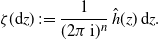 \begin{equation}
{\zeta}({\mathrm{d}} z)\,:\!=\frac1{(2\pi\,{\mathrm{i}})^n}\,\hat h(z)\,{\mathrm{d}} z.
\label{eqn25}
\end{equation}
Let  $H\in{\mathcal{H}}^2$
be the unique (up to indistinguishability) càdlàg real-valued martingale satisfying
 $H_t={\mathrm{E}}[{\eta}\mid{\mathcal{F}}_t]$
a.s.,
 $t\in[0,T]$
.
Assumption 4.1. There exists an optional function  $
(t,\omega ,z)\mapsto \widetilde{H}{{(\omega ,z)}_{t}}
$
such that
 $\skew3\widetilde H(z)$
has càdlàg paths and
 $\skew3\widetilde H(z)_t={\mathrm{E}}[{\mathrm{e}}^{z^{\top} X_T}|{\mathcal{F}}_t]$
a.s. for every
 $t\in[0,T]$
, for every
 $z\in{\mathcal{S}}$
.
Proposition 4.2. Let Assumption 4.1 hold. Then  $\skew3\widetilde H(z)\in{\mathcal{H}}^2_{{\mathbb{C}}}$
, for every
 $z\in{\mathcal{S}}$
, and
 $\sup_{z\in{\mathcal{S}}}{\mathrm{E}}[|\skew3\widetilde H(z)_T|^2]<+\infty$
. Furthermore,
 $\widehat H\in{\mathcal{H}}^2_{\mathbb{C}}$
, where
 $\widehat H_t\,:\!=\int_{\mathcal{S}} \skew3\widetilde H(z)_t {\zeta}({\mathrm{d}} z)$
, and
 $\widehat H$
and H are indistinguishable.
Proof. From Assumption 4.1,  $\left( t,\omega \right)\mapsto \widetilde{H}{{\left( \omega ,z \right)}_{t}}$
is càdlàg and hence
 $\skew3\widetilde H(z)\in{\mathcal{H}}^2_{\mathbb{C}}$
for each
 $z\in{\mathcal{S}}$
, since
 $\skew3\widetilde H(z)_t={\mathrm{E}}[{\mathrm{e}}^{z^{\top} X_T}|{\mathcal{F}}_t]$
a.s. for every
 $t\in[0,T]$
and
 $z\in{\mathcal{S}}$
. Furthermore,
 $\left( t,\omega ,z \right)\mapsto \widetilde{H}{{(\omega ,z)}_{t}}$
is optional and
 $
|\skew3\widetilde H(z)_t|^2\leq \skew3\widetilde H(2R)_t\in L^1({\mathrm{P}})$
holds, a.s., for every
 $t\in[0,T]$
, for every
 $z\in{\mathcal{S}}$
. This yields
 $\sup_{z\in{\mathcal{S}}}{\mathrm{E}}[|\skew3\widetilde H(z)_t|^2]<+\infty$
,
 $t\in[0,T]$
. By Lemma 4.1, we get
 $\widehat H\in{\mathcal{H}}^2_{\mathbb{C}}$
. The identity
 $H_t={\mathrm{E}}[{\eta}|{\mathcal{F}}_t]=\widehat H_t$
holds a.s. and for every
 $t\in[0,T]$
by Fubini’s theorem. This yields that H and
 $\widehat H$
are modifications and, therefore,
 $\widehat H$
is, in particular, real-valued. Since H and
 $\widehat H$
are a.s. càdlàg and modifications, they are indistinguishable. The proof is complete.
Let  $S\in{\mathcal{H}}^2$
describe the price process of some traded asset. We stress that S is a real-valued process. Theorem 4.1 below shows that the Fourier representation (4.5) of
 ${\eta}$
and the GKW decomposition of
 ${\eta}$
with respect to S can be interchanged.
Theorem 4.1. Let  $S\in{\mathcal{H}}^2$
, let
 ${\eta}=h(X_T)\in L^2({\mathrm{P}})$
have the Fourier representation given in (4.5) and (4.6), and let
 $(\vartheta, L)$
denote the GKW decomposition of
 ${\eta}$
with respect to S. Let Assumption 4.1 hold and let
 $(\vartheta(z),L(z))$
be the GKW decomposition of
 $\skew3\widetilde H(z)$
with respect to S, for every
 $z\in{\mathcal{S}}$
, where
 $\skew3\widetilde H$
is the optional function in Assumption 4.1. Let, moreover,
 $\left( t,\omega ,z \right)\mapsto \widetilde{\vartheta }{{\left( \omega ,z \right)}_{t}}$
be a predictable function such that
 $\widetilde\vartheta({\omega},z)_t=\vartheta({\omega},z)_t$
 $
\text{P}\otimes \text{d}\left\langle S,S \right\rangle
$
-a.e. for every
 $z\in{\mathcal{S}}$
.
(i) We have  $\widetilde{\vartheta }\in {{L}^{2}}(\widetilde{\mathcal{P}},\text{P}\otimes \left\langle S,S \right\rangle \otimes \zeta)$
,
 $\int_{\mathcal{S}}\widetilde\vartheta(z){\zeta}({\mathrm{d}} z)\in L^2(S)$
, and there exists an optional function
 $
(t,\omega ,z)\mapsto \widetilde{Y}{{(\omega ,z)}_{t}}
$
such that
 $\widetilde Y(z)$
is a version of
 $\int_0^{\cdot} \widetilde\vartheta(z)_s{\,\mathrm{d}} S_s$
(and hence of
 $\int_0^{\cdot} \vartheta(z)_s{\,\mathrm{d}} S_s$
) for every
 $z\in{\mathcal{S}}$
and
 \begin{equation}
\int_{0}^{t}{\int_{\mathcal{S}}{\widetilde{\vartheta }{{(z)}_{s}}\zeta (\text{d}z)\text{d}{{S}_{s}}}}=\int_{\mathcal{S}}{\widetilde{Y}{{(z)}_{t}}\zeta (\text{d}z),}\quad a.s.,for all\ t\in [0,T].
\label{eqn26}
\end{equation}
(ii) There exists an optional function  $
(t,\omega ,z)\mapsto \text{ }\widetilde{L}{{(\omega ,z)}_{t}}
$
such that
 $\widetilde L(z)$
is a version of L(z), for every
 $z\in{\mathcal{S}}$
. Furthermore,
 $\sup_{z\in{\mathcal{S}}}{\mathrm{E}}[|\widetilde L(z)_t|^2]<+\infty$
,
 $t\in[0,T]$
, and
 \begin{equation}
{{L}_{t}}=\int_{\mathcal{S}}{\text{ }}\widetilde{L}{{(z)}_{t}}\zeta (\text{d}z),\quad \text{a}\text{.s}\text{.},\ for all\ t\in [0,T].
\label{eqn27}
\end{equation}
(iii) The GKW decomposition of  $H\in{\mathcal{H}}^2$
,
 $H_t={\mathrm{E}}[{\eta}\mid{\mathcal{F}}_t]$
a.s.,
 $t\in[0,T]$
, is
 \begin{equation}
H=H_0+\int_0^{\cdot}\int_{\mathcal{S}}\widetilde\vartheta(z)_s\zeta({\mathrm{d}} z){\,\mathrm{d}} S_s+L ,
\label{eqn28}
\end{equation}
and  $\vartheta$
is given by
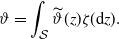 \begin{equation}
\vartheta=\int_{\mathcal{S}}\widetilde\vartheta(z){\zeta}({\mathrm{d}} z).
\label{eqn29}
\end{equation}
Proof. First, we observe that, for every  $z\in{\mathcal{S}}$
, the identity
 \[
{\mathrm{E}}[|\skew3\widetilde H(z)_t|^2]={\mathrm{E}}\left[\Big|\int_0^{\cdot}\vartheta_s(z){\,\mathrm{d}} S_s\Big|^2+|L(z)_t|^2+|\skew3\widetilde H(z)_0|^2\right]
\]
holds. Hence, Proposition 4.2 implies that
 \begin{equation}
\sup_{z\in{\mathcal{S}}}{\mathrm{E}}\left[\Big|\int_0^t\vartheta_s(z){\,\mathrm{d}} S_s\Big|^2\right]<+\infty\,,\qquad \sup_{z\in{\mathcal{S}}}{\mathrm{E}}\Big[|L(z)_t|^2\Big]<+\infty, \quad t\in[0,T].
\label{eqn30}
\end{equation}
We now verify (i). The stochastic integrals  $\int_0^{\cdot}\vartheta_s(z){\,\mathrm{d}} S_s$
and
 $\int_0^{\cdot}\widetilde\vartheta_s(z){\,\mathrm{d}} S_s$
are indistinguishable, for every
 $z\in{\mathcal{S}}$
. So, from (4.11), we get
 $\sup_{z\in{\mathcal{S}}}{\mathrm{E}}[|\int_0^ t\widetilde\vartheta_s(z){\,\mathrm{d}} S_s|^2]<+\infty$
,
 $t\in[0,T]$
. From Tonelli’s theorem and Itô’s isometry, we then have
 \[
\begin{split}
\text{E}\left[ \int_{0}^{T}{\int_{\mathcal{S}}{|}}\widetilde{\vartheta }{{(z)}_{t}}{{|}^{2}}|\zeta |(\text{d}z)\text{d}{{\left\langle S,S \right\rangle }_{t}} \right]&=\int_{\mathcal{S}}{\text{E}}\left[ \int_{0}^{T}{|}\widetilde{\vartheta }{{(z)}_{t}}{{|}^{2}}\text{d}{{\left\langle S,S \right\rangle }_{t}} \right]|\zeta |(\text{d}z)\\
&\le |\zeta |(\mathcal{S})\underset{z\in \mathcal{S}}{\mathop{\sup }}\,\text{E}\left[ |\int_{0}^{T}{\widetilde{\vartheta }(z)\text{d}{{S}_{s}}{{|}^{2}}} \right]<+\infty ,
\end{split}
\]
which shows that  $
\widetilde{\vartheta }\in {{L}^{2}}(\widetilde{\mathcal{P}},\text{P}\otimes \left\langle S,S \right\rangle \otimes \zeta)
$
. Therefore, applying Fubini’s theorem yields that
 $z\mapsto\widetilde\vartheta({\omega},z)_t\in L^2({\zeta})$
 $
\text{P}\otimes \left\langle S,S \right\rangle
$
-a.e., and that
 $(t,{\omega})\mapsto\int_{\mathcal{S}}|\widetilde\vartheta({\omega},z)_t|^2|{\zeta}|({\mathrm{d}} z)$
is predictable and belongs to
 $
{{L}^{1}}(\mathcal{P},\text{P}\otimes \left\langle S,S \right\rangle)
$
. So,
 $\int_{\mathcal{S}}\widetilde\vartheta(z){\zeta}({\mathrm{d}} z)\in L^2(S)$
. To see (4.7), we apply the stochastic Fubini theorem as in [20, Theorem 3(a) and Corollary 2]: There exists an optional function
 $\left( t,\omega ,z \right)\mapsto \widetilde{Y}{{\left( \omega ,z \right)}_{t}}$
such that
 $\widetilde Y(z)$
is a version of
 $\int_0^{\cdot}\widetilde\vartheta(z)_s {\,\mathrm{d}} S_s$
, for every
 $z\in{\mathcal{S}}$
, and we have the identity (4.7). The proof of (i) is complete. We now verify (ii) and (iii). We define
 $\widetilde L({\omega},z)_t\,:\!=\skew3\widetilde H({\omega},z)_t-\skew3\widetilde H(z)_0-\widetilde Y({\omega},z)_t$
, for every
 $(t,\omega ,z)\in \widetilde{\Omega}$
. Since
 $\widetilde L(z)_t=\skew3\widetilde H(z)_t-\skew3\widetilde H(z)_0-\int_0^{\cdot}\widetilde \vartheta(z)_s{\,\mathrm{d}} S_s$
,
 $\widetilde Y(z)$
being a version of
 $\int_0^{\cdot}\widetilde \vartheta(z)_s{\,\mathrm{d}} S_s$
for every
 $z\in{\mathcal{S}}$
, we obtain that
 $\widetilde L(z)$
is a version of L(z) for every
 $z\in{\mathcal{S}}$
. Hence, (4.11) yields the estimate
 $\sup_{z\in{\mathcal{S}}}{\mathrm{E}}[|\widetilde L(z)_t|]<+\infty$
for every
 $t\in[0,T]$
. Therefore, since
 $\widetilde L$
is optional, by Lemma 4.1,
 $\widehat L_t=\int_{\mathcal{S}} \widetilde L(z)_t{\zeta}({\mathrm{d}} z)$
is a square-integrable martingale. We denote by
 $L^{\ast}$
a càdlàg version of
 $\widehat L$
. We can now compute a.s., and for every
 $t\in[0,T]$
,
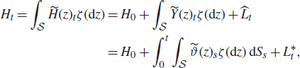 \begin{align}
& {{H}_{t}}=\int_{\mathcal{S}}{\widetilde{H}{{(z)}_{t}}\zeta (dz)}={{H}_{0}}+\int_{\mathcal{S}}{\widetilde{Y}{{(z)}_{t}}\zeta (dz)}+{{\widehat{L}}_{t}} \\
&={{H}_{0}}+\int_{0}^{t}{\int_{\mathcal{S}}{\widetilde{\vartheta }{{(z)}_{s}}\zeta (dz)}}\,\text{d}{{S}_{s}}+L_{t}^{*}, \\
\end{align}
where in the first equality we used Proposition 4.2. But the left-hand side and the right-hand side of the last equality in (4.12) are càdlàg. Hence, they are indistinguishable. To prove (4.9), it remains to show that  $L^{\ast}$
is orthogonal to S. This yields
 $L=L^{\ast}$
. By Tonelli’s theorem and Hölder’s inequality we obtain, for every
 $t\in[0,T]$
,
 $
{\mathrm{E}}[\!\int_{\mathcal{S}} |S_t\widetilde L(z)_t||{\zeta}|({\mathrm{d}} z)]<+\infty
$
. Since SL(z) is a martingale for every
 $z\in{\mathcal{S}}$
,
 $S\widetilde L(z)$
is a martingale for every
 $z\in{\mathcal{S}}$
too,
 $\widetilde L(z)$
being a version of L(z) for every
 $z\in{\mathcal{S}}$
. By Fubini’s theorem, we get, a.s., for every
 $0\leq s\leq t\leq T$
,
 \[
\begin{split}
{\mathrm{E}}[S_t L^{\ast}_t\mid{\mathcal{F}}_s]&={\mathrm{E}}[S_t \widehat L_t\mid{\mathcal{F}}_s]=\int_{\mathcal{S}}{\mathrm{E}}[S_t \widetilde L(z)_t\mid{\mathcal{F}}_s]{\zeta}({\mathrm{d}} z)=S_sL^{\ast}_s.
\end{split}
\]
So,  $L^{\ast}$
is orthogonal to S, and (4.9) and (4.8) hold. From (4.9) we get (4.10) because of
 $
\vartheta =\text{d}\left\langle S,H \right\rangle /\text{d}\left\langle S,S \right\rangle =\int_{\mathcal{S}}{\widetilde{\vartheta }(z)\zeta (\text{d}z)}
$
. The proof is complete.
Let  ${\eta}^{\kern1ptj}$
be a real-valued square-integrable European option with GKW decomposition
 $(\vartheta^{\kern1ptj}, L^{\kern1ptj})$
with respect to S,
 $j=1,2$
. In the following theorem we compute
 $\left\langle {{L}^{1}},{{L}^{2}} \right\rangle$
assuming that
 ${\eta}^{\kern1ptj}=h^{\kern1ptj}(X_T)$
and
 $h^{\kern1ptj}$
has the representation given in (4.5) and (4.6) on
 ${\mathcal{S}}^{\kern1ptj}\,:\!=\{z\in{\mathbb{C}}^n\,:\, {\mathrm{Re}}(z)=R^{\kern1ptj}\}$
with
 ${\mathrm{E}}[\!\exp(2(R^{\kern1ptj})^{\top} X_T)]<+\infty$
,
 $j=1,2$
. We use the notation
 ${\mathcal{S}}\,:\!={\mathcal{S}}^1\cup{\mathcal{S}}^2$
. We also introduce
 $\overline{\Omega}\,:\!=[0,T]\times{\Omega}\times{\mathcal{S}}^1\times{\mathcal{S}}^2$
and
 $\overline{\mathcal{P}}\,:\!={\mathcal{P}}\otimes{\mathcal{B}}({\mathcal{S}}^1)\otimes{\mathcal{B}}({\mathcal{S}}^2)$
.
Theorem 4.2. Let  ${\eta}^{\kern1ptj}\in L^2({\mathrm{P}})$
have the representation (4.5) on
 ${\mathcal{S}}^{\kern1ptj}$
with respect to the measure
 ${\zeta}^{\kern1ptj}$
and let
 $(\vartheta^{\kern1ptj}, L^{\kern1ptj})$
be the GKW decomposition of
 ${\eta}^{\kern1ptj}$
with respect to S,
 $j=1,2$
. Let
 $\skew3\widetilde H$
be the optional mapping in Assumption 4.1 with
 ${\mathcal{S}}\,:\!={\mathcal{S}}^1\cup{\mathcal{S}}^2$
and with the following measurability assumptions: The restriction of
 $\skew3\widetilde H$
to
 $[0,T]\times{\Omega}\times{\mathcal{S}}^{\kern1ptj}$
is optional with respect to
 ${\mathcal{S}}^{\kern1ptj}$
,
 $j=1,2$
. Let
 $(\vartheta(z),L(z))$
be the GKW decomposition of
 $\skew3\widetilde H(z)$
with respect to S for
 $z\in{\mathcal{S}}$
and assume that there exists a mapping
 $\widetilde \vartheta$
on
 $[0,T]\times{\Omega}\times{\mathcal{S}}$
such that
 $\widetilde\vartheta({\omega},z)_t=\vartheta({\omega},z)_t$
 $\text{P}\otimes \left\langle S,S \right\rangle$
-a.e. for every
 $z\in{\mathcal{S}}$
and the restriction of
 $\widetilde\vartheta$
to
 $[0,T]\times{\Omega}\times{\mathcal{S}}^{\kern1ptj}$
is predictable with respect to
 ${\mathcal{S}}^{\kern1ptj}$
,
 $j=1,2$
.
(i) Then there exists an optional mapping  $\widetilde L$
on
 $[0,T]\times{\Omega}\times{\mathcal{S}}$
such that the restriction of
 $\widetilde L$
to
 $[0,T]\times{\Omega}\times{\mathcal{S}}^{\kern1ptj}$
is optional with respect to
 ${\mathcal{S}}^{\kern1ptj}$
,
 $\widetilde L(z)$
is a version of L(z), for every
 $z\in{\mathcal{S}}$
, and
 $L^ j_t=\int_{{\mathcal{S}}^{\kern1ptj}}\widetilde L(z)_t{\zeta}^{\kern1ptj}({\mathrm{d}} z)$
a.s. for every
 $t\in[0,T]$
,
 $j=1,2$
.
(ii) If the function  $
(t,\omega ,{{z}_{1}},{{z}_{2}})\mapsto {{\left\langle L({{z}_{1}})L({{z}_{2}}) \right\rangle }_{t}}(\omega)$
on
 $\overline{\Omega}$
is
 $\overline{\mathcal{P}}$
-measurable then so is
 $
(t,\omega ,{{z}_{1}},{{z}_{2}})\mapsto \text{Tv}{{(\left\langle L({{z}_{1}}),L({{z}_{2}}) \right\rangle )}_{t}}(\omega )
$
, and
 \begin{equation}\begin{split}
\text{E}[{{\int }_{{{\mathcal{S}}^{1}}}}{{\int }_{{{\mathcal{S}}^{2}}}}\text{Tv}{{(\left\langle L({{z}_{1}}),L({{z}_{2}}) \right\rangle )}_{T}}|{{\zeta }^{2}}|(\text{d}{{z}_{2}})|{{\zeta }^{1}}|(\text{d}{{z}_{1}})]<+\infty.
\end{split}
\label{eqn31}
\end{equation}
Moreover,  $
\int_{{{\mathcal{S}}^{1}}}{\int_{{{\mathcal{S}}^{2}}}{\left\langle L({{z}_{1}})L({{z}_{2}}) \right\rangle }}{{\zeta }^{2}}(\text{d}{{z}_{2}}){{\zeta }^{1}}(\text{d}{{z}_{1}})
$
is a predictable process and
 \begin{equation}
\left\langle {{L}^{1}},{{L}^{2}} \right\rangle =\int_{{{\mathcal{S}}^{1}}}{\int_{{{\mathcal{S}}^{2}}}{\left\langle L({{z}_{1}}),L({{z}_{2}}) \right\rangle }}{{\zeta }^{2}}(\text{d}{{z}_{2}}){{\zeta }^{1}}(\text{d}{{z}_{1}}).
\label{eqn32}
\end{equation}
(iii) If  $\widetilde K$
is a
 $\overline{\mathcal{P}}$
-measurable function on
 $\overline{\Omega}$
such that
 $\int_0^T|\widetilde K({\omega},z_1,z_2)_s|{\,\mathrm{d}} s<+\infty$
, for
 $
(\omega ,{{z}_{1}},{{z}_{2}})\in \Omega \times {{\mathcal{S}}^{1}}\times {{\mathcal{S}}^{2}}
$
, and
 $$
{{\left\langle L({{z}_{1}})L({{z}_{2}}) \right\rangle }_{t}}(\omega )=\int_{0}^{t}{\text{ }}\widetilde{K}{{(\omega ,{{z}_{1}},{{z}_{2}})}_{s}}\text{d}s,$$
then  $\widetilde K$
is
 $\overline{\mathcal{P}}$
-measurable,
 $\widetilde K\in L^1(\overline{\mathcal{P}},{\mathrm{P}}\otimes{\mathrm{Leb.}}\otimes{\zeta}^1\otimes{\zeta}^2)$
,
 $$
\left\langle {{L}^{1}},{{L}^{2}} \right\rangle =\int_{0}^{\cdot }{\int_{{{\mathcal{S}}^{1}}}{\int_{{{\mathcal{S}}^{2}}}{\widetilde{K}{{({{z}_{1}},{{z}_{2}})}_{s}}{{\zeta }^{2}}(\text{d}{{z}_{2}}){{\zeta }^{1}}(\text{d}{{z}_{1}})\text{d}s}}}$$
and  $
\text{E}[{{\left\langle {{L}^{1}},{{L}^{2}} \right\rangle }_{T}}]=\int_{0}^{T}{\int_{{{\mathcal{S}}^{1}}}{\int_{{{\mathcal{S}}^{2}}}{\text{E}}}}[\text{ }\widetilde{K}{{({{z}_{1}},{{z}_{2}})}_{s}}]{{\zeta }^{2}}(\text{d}{{z}_{2}}){{\zeta }^{1}}(\text{d}{{z}_{1}})\text{d}s
$
.
Notice that the process  $\left\langle {{L}^{1}},{{L}^{2}} \right\rangle$
in Theorem 4.2 is real valued, while
 $\left\langle L({{z}_{1}}),({{z}_{2}}) \right\rangle$
is complex valued,
 $z_j\in{\mathcal{S}}^{\kern1ptj}$
,
 $j=1,2$
.
Proof of Theorem 4.2. We have  $\sup_{z\in{\mathcal{S}}^{\kern1ptj}}{\mathrm{E}}[|\skew3\widetilde H(z)_T|^2]<+\infty$
,
 $j=1,2$
; this means that
 $\sup_{z\in {\mathcal{S}}}{\mathrm{E}}[|\skew3\widetilde H(z)_T|^2]<+\infty$
. To see (i), it is enough to apply Theorem 4.1 to
 ${\mathcal{S}}^1$
and
 ${\mathcal{S}}^2$
to find a functional
 $\widetilde L^{\kern1ptj}$
which is optional with respect to
 ${\mathcal{S}}^{\kern1ptj}$
, such that
 $\widetilde L^{\kern1ptj}(z)$
is a version of L(z) for
 $z\in{\mathcal{S}}^{\kern1ptj}$
and
 $L^{\kern1ptj}_t=\int_{{\mathcal{S}}^{\kern1ptj}}\widetilde L^{\kern1ptj}(z){\zeta}^{\kern1ptj}({\mathrm{d}} z)$
a.s.,
 $t\in[0,T]$
,
 $j=1,2$
. Since
 ${\mathcal{S}}^1$
and
 ${\mathcal{S}}^2$
are either disjoint or identical, we define
 $\widetilde L$
on
 ${\mathcal{S}}$
setting
 $\widetilde L({\omega},t,z)\,:\!=\widetilde L^{\kern1ptj}({\omega},z)_t$
, for
 $(t,{\omega},z)$
in
 $[0,T]\times{\Omega}\times{\mathcal{S}}^{\kern1ptj}$
,
 $j=1,2$
, and
 $\widetilde L$
has the desired properties. We now come to (ii). By (4.11), we get
 $\sup_{z\in {\mathcal{S}}^{\kern1ptj}}{\mathrm{E}}[|L(z)_t|^2]\leq\sup_{z\in {\mathcal{S}}}{\mathrm{E}}[|L(z)_t|^2]<+\infty$
,
 $t\in[0,T]$
,
 $j=1,2$
, and (4.13) can be proven as (4.1). From (4.13) we see that
 $\int_{{{\mathcal{S}}^{1}}}{\int_{{{\mathcal{S}}^{2}}}{\left\langle L({{z}_{1}}),L({{z}_{2}}) \right\rangle }}{{\zeta }^{2}}(\text{d}{{z}_{2}}){{\zeta }^{1}}(\text{d}{{z}_{1}})$
is defined for every
 $t\in[0,T]$
a.s. and it is a predictable process of finite variation starting at zero. By the properties of
 $\widetilde L$
, the mapping
 $(t,\omega ,{{z}_{1}},{{z}_{2}})\mapsto \widetilde{L}{{(\omega ,{{z}_{1}})}_{t}}\widetilde{L}{{(\omega ,{{z}_{2}})}_{t}}$
on
 $\overline{\Omega}$
is
 ${\mathrm{P}}\otimes|{\zeta}^1|\otimes|{\zeta}^2|$
-integrable. Hence, since
 $
\widetilde{L}({{z}_{1}})\widetilde{L}({{z}_{2}})-\left\langle \widetilde{L}({{z}_{1}})\widetilde{,L}({{z}_{2}}) \right\rangle$
is a martingale, applying Fubini’s theorem, we see that
 $
{{L}^{1}}{{L}^{2}}-\int_{{{\mathcal{S}}^{1}}}{\int_{{{\mathcal{S}}^{2}}}{\left\langle L({{z}_{1}}),L({{z}_{2}}) \right\rangle }}{{\zeta }^{2}}(\text{d}{{z}_{2}}){{\zeta }^{1}}(\text{d}{{z}_{1}})
$
is a martingale. Thus, we get (4.14). The proof of (iii) is similar to the proof of Proposition 4.1(iii), and is therefore omitted. The proof is complete.
We now combine the results of this section with those of Section 3 for semimartingales with absolutely continuous characteristics. Let us consider the factor process  $X=(X^1,\ldots,X^n)^{\top}$
and let
 $R^{\kern1ptj}\in{\mathbb{R}}$
be such that
 ${\mathrm{E}}[\!\exp(2R^{\kern1ptj} X_T^ 1)]<+\infty$
. We define
 ${\mathcal{S}}^{\kern1ptj}\,:\!=\{z\in{\mathbb{C}}\,:\, {\mathrm{Re}}(z)=R^{\kern1ptj}\}$
,
 $j=1,\ldots,d$
, and set
 ${\mathcal{S}}\,:\!=\bigcup_{j=1}^d{\mathcal{S}}^{\kern1ptj}$
.
Theorem 4.3. Let X be a locally square-integrable semimartingale with differential characteristics (b,c,F), and let  $S={\mathrm{e}}^{X^1}\in{\mathcal{H}}^2$
. Let
 ${\eta}^{\kern1ptj}=h^{\kern1ptj}(S_T)=(h^{\kern1ptj}\circ\exp)(X^1_T)$
be a real-valued square-integrable European option, let
 $h^{\kern1ptj}\circ\exp$
have the representation given in (4.5) and (4.6) on
 ${\mathcal{S}}^{\kern1ptj}$
, and let
 $(\vartheta^{\kern1ptj},L^{\kern1ptj})$
be the GKW decomposition of
 ${\eta}^{\kern1ptj}$
with respect to S,
 $j=1,\ldots,d$
. Additionally:
(i) Let  $f\,:\,[0,T]\times{\mathbb{R}}^n\times{\mathcal{S}} \rightarrow{\mathbb{C}} $
be such that the restriction of f to
 $[0,T]\times{\mathbb{R}}^n\times{\mathcal{S}}^{\kern1ptj}$
is
 ${\mathcal{B}}([0,T])\otimes{\mathcal{B}}({\mathbb{R}}^n)\otimes{\mathcal{B}}({\mathcal{S}}^{\kern1ptj})$
-measurable,
 $j=1,\ldots,d$
,
 $f(\cdot,\cdot, z)\in C^{1,2}([0,T]\times{\mathbb{R}}^n)$
, for
 $z\in{\mathcal{S}}$
, and
 $\skew3\widetilde H({\omega},z)_t=f(t,X_t({\omega}),z)$
,
 $\skew3\widetilde H(z)_t={\mathrm{E}}[{\mathrm{e}}^{zX^1_T}\mid{\mathcal{F}}_t]$
, a.s.,
 $t\in[0,T]$
,
 $z\in{\mathcal{S}}$
.
(ii) We define the complex-valued function  $W(t,{\omega},x,z)\,:\!=f(t,x+X_{t-}({\omega}),z)-f(t,$
 $X_{t-}({\omega}),z)$
, for
 $z\in{\mathcal{S}}$
, and assume that
 $\int_E|W(t,{\omega},x,z)|^2 F_t({\omega},{\mathrm{d}} x)<+\infty$
, for every
 $(t,{\omega},z)\in[0,T]\times{\Omega}\times{\mathcal{S}}$
, and that
 $\int_E({\mathrm{e}}^{ x_1}-1)^2F_t({\omega},{\mathrm{d}} x)<+\infty$
,
 $\xi_t({\omega})>0$
for every
 $(t,{\omega})\in[0,T]\times{\Omega}$
(see Corollary 3.1(i) for the definition of the process
 $\xi$
).
(iii) Let  $(\vartheta(z),L(z))$
denote the GKW decomposition of
 $\skew3\widetilde H(z)$
with respect to S, for
 $z\in{\mathcal{S}}$
, and let
 $(t,{\omega},z)\mapsto\widetilde\vartheta({\omega},z)_t$
be the function defined on the right-hand side of (3.14) in terms of
 $f(t,X_{t-}({\omega}),z)$
and
 $W(t,{\omega},x,z)$
(see (ii) above), that is,
 \[
\widetilde\vartheta(z)_t=\frac{1}{S_{t-}\xi_t}\bigg(\sum_{k=1}^n\partial_{x_k}f(t,X_{t-},z)c^{1k}_t+\int_E({\mathrm{e}}^{x_1}-1)W(t,x,z)F_t({\mathrm{d}} x)\bigg),\quad z\in{\mathcal{S}}.
\]
Claim 1. The mapping  $
(t,\omega )\mapsto \text{ }\widetilde{H}{{(\omega ,z)}_{t}}
$
is càdlàg, for
 $z\in{\mathcal{S}}$
, and the restriction of
 $\skew3\widetilde H$
to
 ${\mathcal{S}}^{\kern1ptj}$
is optional with respect to
 ${\mathcal{S}}^{\kern1ptj}$
,
 $j=1,\ldots,d$
. Furthermore,
 $\widetilde\vartheta(z)=\vartheta(z)$
 $
\text{P}\otimes \text{d}\left\langle S,S \right\rangle
$
-a.e., for
 $z\in{\mathcal{S}}$
, holds, and the restriction of
 $\widetilde\vartheta$
to
 ${\mathcal{S}}^{\kern1ptj}$
is a predictable function with respect to
 ${\mathcal{S}}^{\kern1ptj}$
,
 $j=1,\ldots,d$
. In particular, the assumptions of Theorem 4.1 are satisfied with respect to
 ${\mathcal{S}}^{\kern1ptj}$
,
 $j=1,\ldots,d$
.
(iv) We denote by  $f^{\kern1ptj}$
and
 $W^{\kern1ptj}$
the complex-valued functions obtained taking the restriction of f and W to
 ${\mathcal{S}}^{\kern1ptj}$
, respectively, so that
 $\skew3\widetilde H({\omega},z)_t=f^{\kern1ptj}(t,X_t({\omega}),z)$
,
 $z\in{\mathcal{S}}^{\kern1ptj}$
,
 $j=1,\ldots,d$
. Let
 $\widetilde K({\omega},z_i,z_j)$
denote the density of
 $
\left\langle L({{z}_{i}}),L({{z}_{j}}) \right\rangle
$
with respect to the Lebesgue measure given in (3.15) (now defined with respect to
 $f^i$
,
 $f^ j$
,
 $W^i$
, and
 $W^{\kern1ptj}$
,
 $i,j=1,\ldots,d$
) and let
 $\int_0^T|\widetilde K({\omega},z_i,z_j)_t|{\,\mathrm{d}} t<+\infty$
for every
 $
(t,\omega ,{{z}_{i}},{{z}_{j}})\in [0,T]\times \Omega \times {{\mathcal{S}}^{i}}\times {{\mathcal{S}}^{j}}
$
, for every
 $i,j=1,\ldots,d$
.
Claim 2. The function  $
(t,\omega ,{{z}_{i}},{{z}_{j}})\mapsto \int_{0}^{t}{\widetilde{K}{{(\omega ,{{z}_{i}},{{z}_{j}})}_{s}}\text{d}s}
$
is predictable with respect to
 ${\mathcal{S}}^ i\times{\mathcal{S}}^{\kern1ptj}$
and we have
 $\text{E}[{{\left\langle {{L}^{i}},{{L}^{j}} \right\rangle }_{T}}]=\int_{0}^{T}{\int_{{{\mathcal{S}}^{i}}}{\int_{{{\mathcal{S}}^{j}}}{\text{E}}}}[\widetilde{K}{{(\omega ,{{z}_{i}},{{z}_{j}})}_{t}}]{{\zeta }^{j}}(\text{d}{{z}_{j}}){{\zeta }^{i}}(\text{d}{{z}_{i}})\text{d}t$
, for
 $i,j=1,\ldots,d$
.
5. Applications
We apply the results of Sections 3 and 4 to two continuous stochastic volatility models, the Heston model, which is affine, and the 3/2 model, which is not, and to a simple model with jumps.
We set up a variance-optimal semi-static hedging strategy for a variance swap  ${\eta}^0$
: Let X be a square-integrable semimartingale and let
 $S={\mathrm{e}}^X\in{\mathcal{H}}^2$
; then
 \begin{equation*}\label{eq:var.sw}
{\eta}^0=[X,X]_T-k,
\end{equation*}
where  $k={\mathrm{E}}[[X,X]_T]$
so that
 ${\mathrm{E}}[{\eta}^0]=0$
.
A basket  $({\eta}^1,\ldots,{\eta}^d)$
of European options written on S is fixed. We assume that
 ${\eta}^{\kern1ptj}\in L^2({\mathrm{P}})$
and
 ${\eta}^{\kern1ptj}=h^{\kern1ptj}(S_T)$
, where
 $h^{\kern1ptj}\circ\exp$
has the representation given in (4.5) and (4.6), with respect to the complex-valued measure
 ${\zeta}^{\kern1ptj}$
on
 ${\mathcal{S}}^{\kern1ptj}=\{z\in{\mathbb{C}}\,:\, {\mathrm{Re}}(z)=R^{\kern1ptj}\}$
,
 ${\mathrm{E}}[\!\exp(2R^{\kern1ptj}X_T)]<+\infty$
,
 $j=1,\ldots,d$
.
5.1. The Heston model
The Heston model for  ${{(X,V)}^{\top }}$
(see [Reference Heston14]) is given by
 \begin{equation*}\label{eq:Heston}
{\mathrm{d}} X_{\,t}=-\frac12 V_{\,t}{\,\mathrm{d}} t+\sqrt{V_{\,t}} {\,\mathrm{d}} W_{\,t}^{\,1},\quad {\mathrm{d}} V_{\,t}=-\lambda(V_{\,t}-\kappa ){\,\mathrm{d}} t+\sigma\sqrt{V_{\,t}} {\,\mathrm{d}} W_{\,t}^{\,2},
\end{equation*}
where  $W^1$
and
 $W^2$
are correlated Brownian motions with
 $
{{\left\langle {{W}^{1}},{{W}^{2}} \right\rangle }_{t}}=\rho t$
,
 $\rho\in[\!-1,1]$
and
 $\lambda,\sigma,\kappa>0$
,
 $2{\lambda}\kappa\geq{\sigma}^2$
so that
 $V_t>0$
. Notice that
 ${{(X,V)}^{\top }}$
is affine and
 \begin{equation}
{\mathrm{E}}[\!\exp( u_1X_T+u_2V_T)\mid{\mathcal{F}}_t]=\exp(\phi_{T-t}(u_1,u_2)+u_1 X_t+\psi_{T-t}(u_1,u_2)V_t)=\!:\,\skew3\widetilde H(z)_t,
\label{eqn33}
\end{equation}
where  $(t,u_1,u_2)\mapsto\phi_t(u_1,u_2)$
and
 $(t,u_1,u_2)\mapsto\psi_t(u_1,u_2)$
are complex-valued functions that can be expressed in terms of elementary functions. See [Reference Heston14], [2, Section 4.2.1], [Reference Albrecher, Mayer, Schoutens and Tistaert1,Reference Keller-Ressel and Mayerhofer19] etc. for concrete expressions, domain of validity, and numerical issues.
For  $z\in{\mathcal{S}}^{\kern1ptj}$
, we have
 $\skew3\widetilde H(z)\in{\mathcal{H}}^2_{\mathbb{C}}$
,
 $j=1,\ldots,d$
. Defining
 $r^0_{z_1,z_2}\,:\!=\phi_t(z_1,0)+\phi_t(z_2,0)$
and
 $r^ 1_{z_1,z_2}\,:\!=\psi_t(z_1,0)+\psi_t(z_2,0)$
for
 $z_1\in{\mathcal{S}}^i$
,
 $z_2\in{\mathcal{S}}^{\kern1ptj}$
, from [18, Equation (5.18)], for
 $t\in[0,T]$
, the random variable
 $V_t\skew3\widetilde H(z_1)_t\skew3\widetilde H(z_2)_t$
is integrable and
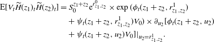 \begin{equation}
\begin{split}
{\mathrm{E}}[V_t\skew3\widetilde H(z_1)_t\skew3\widetilde H(z_2)_t]=&\ S_0^{z_1+z_2}{\mathrm{e}}^{r^0_{z_1,z_2}}\times\exp(\phi_t(z_1+z_2,r^1_{z_1,z_2})\\&+\psi_t(z_1+z_2,r^ 1_{z_1,z_2})V_0)\times\partial_{u_2}[\phi_t(z_1+z_2,u_2)\\
&+\psi_t(z_1+z_2,u_2)V_0]|_{u_2=r^1_{z_1,z_2}}.
\end{split}
\label{eqn34}
\end{equation}
5.1.1. Semi-static variance-optimal hedging
We now compute the quantities A, B, and C defined in (2.4) for the variance swap  ${\eta}^0=\int_0^T V_s{\,\mathrm{d}} s-k$
in the Heston model. We start by computing A.
Proposition 5.1. Setting  ${\alpha}(t)\,:\!={\lambda}^{-1}(1-{\mathrm{e}}^{-{\lambda}(T-t)})$
, we have
 \begin{equation}
A={\sigma}^2(1-\varrho^2)\int_0^T{\alpha}^2(t)[(V_0-\kappa){\mathrm{e}}^{-{\lambda} t}+\kappa]\,{\mathrm{d}} t.
\label{eqn35}
\end{equation}
 \begin{equation}
{\mathrm{E}}[V_s\mid{\mathcal{F}}_t]=\kappa(1-{\mathrm{e}}^{-{\lambda} (s-t)})+{\mathrm{e}}^{-{\lambda} (s-t)}V_t,\quad s\geq t.
\label{eqn36}
\end{equation}
We consider  $H^0\in{\mathcal{H}}^2$
such that
 $H^0_t={\mathrm{E}}[\!\int_0^T V_s{\,\mathrm{d}} s|{\mathcal{F}}_t]$
a.s.,
 $t\in[0,T]$
. By Fubini’s theorem we obtain
 $H^0_t=f^0(t,X_t,V_t,[X,X]_t)$
, where
 $f^0(t,x,v,w)=\tilde{\alpha}(t)+{\alpha}(t)v+w$
, with
 $\tilde{\alpha}(t)\,:\!=\kappa{\lambda}^{-1}({\lambda}(T-t)-1+{\mathrm{e}}^{-{\lambda}(T-t)})$
and
 ${\alpha}(t)$
as above,
 $t\in[0,T]$
. We can now apply Corollary 3.1(ii) with
 $Y^i=H^0$
,
 $f^i=f^0$
,
 $i=1,2$
, and
 $
{{({{X}^{1}},{{X}^{2}},{{X}^{3}})}^{\top }}={{(X,V,[X,X])}^{\top }}
$
. The only relevant derivative is
 $\partial_v f^0={\alpha}(t)$
. Taking the expectation in (3.16), and applying Fubini’s theorem and (5.4) with
 $t=0$
, we get (5.1). The proof is complete.
We stress that according to Corollary 3.1(ii) we have  $\vartheta^0_t=\rho{\sigma}{\alpha}(t)S_t^{-1}$
. As a next step, we compute the vector B in (2.4).
Proposition 5.2. For  $B=(B^1,\ldots,B^d)^{\top}$
we have
 \[
B^{\kern1ptj}={\sigma}^2(1-\varrho^2)\int_0^T\int_{{\mathcal{S}}^{\kern1ptj}}{\alpha}(t)E(t,z)\psi_{T-t}(z,0){\zeta}^{\kern1ptj}({\mathrm{d}} z){\,\mathrm{d}} t,
\]
where  ${\alpha}(t)={\lambda}^{-1}(1-{\mathrm{e}}^{-{\lambda}(T-t)})$
and the explicit expression of
 $E(t,z)\,:\!={\mathrm{E}}[\skew3\widetilde H(z)_tV_t]$
is given by (5.2) with
 $z_1=z\in{\mathcal{S}}^{\kern1ptj}$
,
 $j=1,\ldots,d$
, and
 $z_2=0$
.
Because of (5.1),  $\widetilde K(z)_t\,:\!={\sigma}^2(1-\rho^2){\alpha}(t)\psi_{T-t}(z,0)\skew3\widetilde H(z)_tV_t$
is a predictable function with respect to each
 ${\mathcal{S}}^{\kern1ptj}$
,
 $j=1,\ldots,d$
. Furthermore, it is continuous in t. Because of (5.1) and Theorem 4.3, the assumptions of Theorem 4.1 are satisfied with respect to
 ${\mathcal{S}}^{\kern1ptj}$
, for each
 $j=1,\ldots,d$
, so we have
 $L^ j_t=\int_{{\mathcal{S}}^{\kern1ptj}}\widetilde L(z){\zeta}^{\kern1ptj}({\mathrm{d}} z)$
, a.s.,
 $t\in[0,T]$
. Since
 $\sup_{z\in{\mathcal{S}}^{\kern1ptj}}{\mathrm{E}}[|\widetilde L(z)_t|^2]<+\infty$
,
 $t\in[0,T]$
,
 $j=1,\ldots,d$
, from Proposition 4.1(iii) we get
 $${{B}^{j}}=\text{E}[{{\left\langle {{L}^{0}},{{L}^{j}} \right\rangle }_{T}}]={{\sigma }^{2}}(1-{{\rho }^{2}})\int_{0}^{T}{\int_{{{\mathcal{S}}^{j}}}{\alpha }}(t){{\psi }_{T-t}}(z,0)\text{E}[\widetilde{H}{{(z)}_{t}}{{V}_{t}}]{{\zeta }^{j}}(\text{d}z)\text{d}t.$$
Finally, from (5.2) we get the explicit expression of  ${\mathrm{E}}[\skew3\widetilde H(z)_tV_t]$
.
Proposition 5.3. For  $C=(C^{ij})_{i,j=1,\ldots,d}$
, we have
 \[\begin{split}
C^{ij}={\sigma}^2(1-\varrho^2)\int_0^T\int_{{\mathcal{S}}^i}\int_{{\mathcal{S}}^{\kern1ptj}}\psi_{T-t}(z_1,0)\psi_{T-t}(z_2,0)J(t,z_1,z_2){\zeta}^{\kern1ptj}({\mathrm{d}} z_2){\zeta}^i({\mathrm{d}} z_1){\,\mathrm{d}} t,
\end{split}\]
where  $J(t,z_1,z_2)\,:\!={\mathrm{E}}[\skew3\widetilde H(z_1)_t\widetilde H(z_2)_tV_t]$
is given by (5.2),
 $i,j=1,\ldots,d$
.
where,  $(t,{\omega},z_1,z_2)\mapsto\widetilde K({\omega},z_1,z_2)_t$
is
 ${\mathcal{P}}\otimes{\mathcal{B}}({\mathcal{S}}^i)\otimes{\mathcal{B}}({\mathcal{S}}^{\kern1ptj})$
-measurable and continuous in t. Since we have
 $V_t>0$
, the claim follows from Theorem 4.3.
5.2. The 3/2 model
The 3/2 model for  ${{(X,V)}^{\top }}$
is given by
 \begin{equation}
{\mathrm{d}} X_t=-\frac{V_t}{2}{\,\mathrm{d}} t+\sqrt{V_t}{\,\mathrm{d}} W_t^1,\qquad {\mathrm{d}} V_t=V_t({\lambda}-\kappa V_t){\,\mathrm{d}} t+{\sigma} V_t^{3/2}{\,\mathrm{d}} W^ 2_t,\quad V_0>0,
\label{eqn37}
\end{equation}
where  $W^{1}$
and
 $W^{2}$
are Brownian motions with
 ${{\left\langle {{W}^{1}},{{W}^{2}} \right\rangle }_{t}}=\rho t$
,
 $\rho\in[\!-1,1]$
. We assume
 $\kappa>0$
, which ensures both non-explosion of V (see [10, Equation (3)]) and
 $V_t>0$
,
 $t\in[0,T]$
. The two-dimensional semimartingale
 ${{(X,V)}^{\top }}$
given by (5.5) is not an affine process. For the computation of the conditional moment-generating function we mainly refer to [Reference Grasselli13], that is, we regard the 3/2 model as a special case of the so-called 4/2 model. More precisely, setting
 $a=0$
,
 $b=1$
, and
 $r=0$
in [13, Equation (2.1)], we get the dynamics of the price process
 $S={\mathrm{e}}^X$
(and hence of
 $X=\log S$
) under the local martingale measure in the 3/2 model. We stress that, denoting by
 $\kappa_G, \theta_G, {\sigma}_G$
the parameters in [13, Equation (2.2)], the relation between
 ${\lambda}$
,
 $\kappa$
, and
 ${\sigma}$
in (5.5) and
 $\kappa_G, \theta_G, {\sigma}_G$
is
 \begin{equation}
\kappa=\kappa_G\theta_G-{\sigma}^2_G,\quad {\lambda}=\kappa_G,\quad {\sigma}=-{\sigma}_G.
\label{eqn38}
\end{equation}
In [17, Proposition 6.3.2.1] the transition density of the process  $R=(R_t)_{t\in[0,T]}$
,
 $R_t\,:\!=1/V_t$
is given. From this, we obtain the density function
 $f_{V_t}(v)$
of
 $V_t$
:
 $f_{V_t}(v)=0$
for
 $v\leq0$
, and for
 $v>0$
 \begin{equation}
\begin{split}
f_{V_t}(v)=&\frac{1}{2v^2}\,\frac{4{\lambda}}{{\sigma}^2({\mathrm{e}}^{{\lambda} t}-1)}\bigg(\frac{V_0}v\bigg)^{q/2}\\&\quad\times\exp\bigg({\lambda}\Big(1+\frac{ q}2\Big)t-\frac{2{\lambda}}{{\sigma}^2({\mathrm{e}}^{{\lambda} t}-1)}\Big(\frac{1}{V_0}+\frac{{\mathrm{e}}^{{\lambda} t}}{v}\Big)\bigg) I_q\bigg(\frac{4{\lambda}{\mathrm{e}}^{\frac{{\lambda}}{2}t}}{{\sigma}^2({\mathrm{e}}^{{\lambda} t}-1)\sqrt{V_0v}}\bigg),
\end{split}
\label{eqn39}
\end{equation}
where  $q\,:\!=2({\kappa}+{\sigma}^2)/{\sigma}^2-1$
and
 $I_p(\cdot)$
denotes the modified Bessel function of the first kind.
From [13, p. 17], denoting by  $M(a,b,\cdot)$
the confluent hypergeometric function, we have
 \begin{equation*}\label{eq:mom.v_t}
\begin{split}
\text{E}[V_{t}^{\eta }]={{\left( \frac{2\lambda {{\text{e}}^{\lambda t}}}{{{\sigma }^{2}}({{\text{e}}^{\lambda t}}-1)} \right)}^{\eta }}\exp \left( -\frac{2\lambda }{{{\sigma }^{2}}({{\text{e}}^{\lambda t}}-1){{V}_{0}}} \right)\frac{\Gamma (q+1-\eta )}{\Gamma (q+1)}\times M\left( q+1-\eta ,q+1,\frac{2\lambda }{{{\sigma }^{2}}({{\text{e}}^{\lambda t}}-1){{V}_{0}}} \right)
\end{split}
\end{equation*}
for  ${\eta}\in{\mathbb{R}}$
such that
 $q+1-{\eta}>0$
, which always holds for
 ${\eta}=2+\delta$
, for some fixed
 $\delta>0$
: In the 3/2 model, contrary to the Heston model,
 $V_t$
does not have finite moments of every order. According to [13, Proposition 3.1], for
 $z\in{\mathbb{C}}$
we have
 $\exp(zX_T)\in L^1({\mathrm{P}})$
if
 ${\mathrm{Re}}(z)\in{\mathcal{A}}_{0,+\infty}$
, where the set
 ${\mathcal{A}}_{0,+\infty}$
is defined in [13, Equation (3.7)].
Let  $\exp(zX_T)$
be integrable,
 $z\in{\mathbb{C}}$
. By the relation
 $M(x,y,z)={\mathrm{e}}^z\,M(y-x,y,-z)$
,
 $z\in{\mathbb{C}}$
, for the confluent hypergeometric function, from [13, Equation (3.3)] with
 $a=0$
and
 $b=1$
, we obtain
 $\skew3\widetilde H(z)_t={\mathrm{E}}[\!\exp(zX_T)\mid{\mathcal{F}}_t]$
, a.s.,
 $t\geq0$
, where
 \begin{equation}
\skew3\widetilde H(z)_t={\mathrm{e}}^{zX_t}g(t,V_t,z),
\label{eqn40}
\end{equation}
and the function g is given by
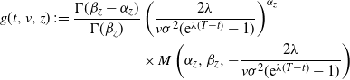 \begin{equation}
\begin{split}
g(t,v,z)\,:\!=\frac{\Gamma({\beta}_z-{\alpha}_z)}{\Gamma({\beta}_z)}&\left(\frac{2{\lambda}}{v{\sigma}^2({\mathrm{e}}^{{\lambda}(T-t)}-1)}\right)^{{\alpha}_z}\\&\times M\left({\alpha}_z,{\beta}_z,-\frac{2{\lambda}}{v{\sigma}^2({\mathrm{e}}^{{\lambda}(T-t)}-1)}\right)
\end{split}
\label{eqn41}
\end{equation}
and  ${\alpha}_z=-\frac12-\frac{\tilde\kappa_z}{{\sigma}^2}+c_z$
,
 ${\beta}_z=1+2c_z$
,
 $\tilde\kappa_z=k-z\varrho{\sigma}$
,
 $c_z\,:\!=\{(\frac12+\frac{\tilde\kappa_z}{{\sigma}^2})^2+\frac{z-z^2}{{\sigma}^2}\}^{1/2}$
.
In the proof of [7, Theorem 3, Section 8], it was shown that  $v\mapsto g(t,v,z)$
(therein
 $\ell$
) solves an ordinary differential equation of the second order and
 $g(T,V_T,z)=1$
. So,
 $t\mapsto\skew3\widetilde H({\omega},z)_t$
is continuous. Taking
 $m_z$
as in [13, Equation (3.5)] with
 $a=0$
and
 $b=1$
, then
 $c_z=\frac{m_z}2$
, by the properties of the confluent hypergeometric function M (x, y, z), and we get:
 \begin{equation}
\begin{split}
\partial_{v} g(t,v,z)=&\frac{{\alpha}_z}{v}(\delta(t,v))^{{\alpha}_z}\frac{\Gamma({\beta}_z-{\alpha}_z)}{\Gamma({\beta}_z)}\\&\times\bigg[\frac{\delta(t,v)}{{\beta}_z}M({\alpha}_z+1,{\beta}_z+1,-\delta(t,v))-M({\alpha}_z,{\beta}_z,-\delta(t,v))\bigg],
\end{split}
\label{eqn42}
\end{equation}
where  $\delta(t,v)\,:\!=\frac{2{\lambda}}{{\sigma}^2({\mathrm{e}}^{{\lambda}(T-t)}-1)v}$
. We require
 $\kappa-\varrho{\sigma}\geq-\frac{{\sigma}^2}{2}$
(i.e., Feller’s condition), which ensures that
 $S={\mathrm{e}}^X$
is a true martingale (see [13, Remark 3.3] with the identification of parameters in (5.6)). To get
 $S\in{\mathcal{H}}^2$
, we require
 $2\in{\mathcal{A}}_{0,+\infty}$
.
We observe that the variance swap  ${\eta}^0$
is square integrable in this model. This follows because, analyzing the explicit expression of the Laplace transform of
 ${\eta}^0$
, which was calculated in [7, Theorem 3] (or [13, Appendix A]), we recognize that it is defined in an open neighborhood of zero.
5.2.1. Variance-optimal semi-static hedging
We now compute the quantities A, B, and C defined in (2.4) for the variance swap  ${\eta}^0=\int_0^T V_s{\,\mathrm{d}} s-k$ in the 3/2 model.
We start by computing A. First, we introduce the function
 \begin{equation}
h^{\prime}(y)=\frac{{\sigma}^2}{2}\Gamma(q){\mathrm{e}}^{-{2/{\sigma}^2y}}y^{-1}{\gamma}^{\ast}\Big(q,-\frac{2}{{\sigma}^2y}\Big),
\label{eqn43}
\end{equation}
where  $\gamma^{\ast}(a,z)\,:\!=\frac1{\Gamma(a)}\int_0^1u^{a-1}{\mathrm{e}}^{-zu}{\,\mathrm{d}} u$
, such that
 $\gamma^{\ast}(a,z)=\frac{z^{-a}}{\Gamma(a)}\,\gamma(a,z)$
,
 $\gamma$
denoting the lower incomplete Gamma function. We then put
 $h(y)\,:\!=\int_0^ yh^{\prime}(x){\,\mathrm{d}} x$
. The function h was introduced in [7, Theorem 4] and this is just a more compact way to write h.
Proposition 5.4. Setting  ${\beta}(t)\,:\!={\lambda}^{-1}({\mathrm{e}}^{{\lambda}(T-t)}-1)$
, we have
 \[
\begin{split}
A&={\sigma}^2(1-\rho^2)\int_0^T\int_0^{\infty}{\beta}(t)^2[h^{\prime}({\alpha}(t)v)]^2v^3f_{V_t}(v)
{\,\mathrm{d}} v\,{\,\mathrm{d}} t,
\end{split}
\]
where  $f_{V_t}(v)$
is as in (5.7) and
 $h^{\prime}$
is from (5.11).
Proof. The process  $(X,V,[X,X])^{\top}$
is a locally square-integrable semimartingale with absolutely continuous characteristics. The second differential characteristic c is given by
 $c_t^{11}=V_t$
,
 $c_t^{12}=\rho{\sigma} V_t^2$
,
 $c_t^{22}={\sigma}^2V_t^3$
, and
 $c_t^{i3}=0$
,
 $i=1,2,3$
. Since
 $[X,X]=\int_0^{\cdot} V_s{\,\mathrm{d}} s$
, we consider
 $H^0\in{\mathcal{H}}^2$
such that
 $H_t^0={\mathrm{E}}[\!\int_0^TV_s{\,\mathrm{d}} s\mid{\mathcal{F}}_t]-k$
a.s.,
 $t\in[0,T]$
. By the Markov property of V and [7, Theorem 4], we get
 $H^0_t+k=f^0(t,X_t,V_t,[X,X]_t)$
, with
 $f^0(t,x,v,w)\,:\!=h({\beta}(t)v)+w$
, and moreover
 $h(y)\,:\!=\int_0^yh^{\prime}(x){\,\mathrm{d}} x$
. The function
 $f^0$
is twice continuously differentiable (see [7, Equation (81)]) and
 $\partial_{v}f^0(t,v,w)={\beta}(t)h^{\prime}({\beta}(t)v)$
. Therefore, by Corollary 3.1(ii), we obtain
 \[
\begin{split}
{{\left\langle {{L}^{0}},{{L}^{0}} \right\rangle }_{T={{\sigma }^{2}}(1-{{\rho }^{2}})}}\int_{0}^{T}{\beta }{{(t)}^{2}}{{[{{h}^{\prime }}(\beta (t){{V}_{t}})]}^{2}}V_{t}^{3}\text{d}t.
\end{split}
\]
Taking the expectation and using Fubini’s theorem yields the result.
We stress that according to Corollary 3.1(ii) we have  $\vartheta^0_t=\rho{\sigma}{\beta}(t)h^{\prime}({\beta}(t)V_t)V_tS_t^{-1}$
.
As the next step, we compute the vector B. The explicit expression of  ${\mathrm{E}}[{\mathrm{e}}^{zX_T}\mid V_t]$
can be obtained from [13, Proposition 4.1], with
 $a=0$
and
 $b=1$
(observe that
 $R_t=V_t^{-1}$
, where
 ${{({{R}_{t}})}_{t\in [0,T]}}$
denotes the volatility process in [13, Equation (2.2)]), and reads
 \begin{equation}
\begin{split}
{\mathrm{E}}[{\mathrm{e}}^{zX_t}\mid V_t]=\exp\bigg(zX_0-z\frac{{\lambda}\rho}{{\sigma}}\,t\bigg)\bigg(\frac{V_t}{V_0}\bigg)^{\frac{z\rho}{{\sigma}}}\;\frac{I_{\frac{2}{{\sigma}^2}\,\sqrt{B_z}}\left(\frac{4{\lambda}{\mathrm{e}}^{\frac{{\lambda}}{2}t}}{{\sigma}^2({\mathrm{e}}^{{\lambda} t}-1)\sqrt{V_0V_t}}\right)}{I_q\left(\frac{4{\lambda}{\mathrm{e}}^{\frac{{\lambda}}{2}t}}{{\sigma}^2({\mathrm{e}}^{{\lambda} t}-1)\sqrt{V_0V_t}}\right)},
\end{split}
\label{eqn44}
\end{equation}
where  $
B_z\,:\!=(\kappa+\frac{{\sigma}^2}{2})^2+2{\sigma}^2[z(\frac{\rho}{{\sigma}}(\kappa+\frac{{\sigma}^2}{2})-\frac12)+\frac{z^2}{2}(1-\rho^2)].
$
Proposition 5.5. For  $B=(B^1,\ldots,B^d)^{\top}$
, setting
 ${\beta}(t)={\lambda}^{-1}({\mathrm{e}}^{{\lambda}(T-t)}-1)$
,
 \[
B^{\kern1ptj}={\sigma}^2(1-\rho^2)\int_0^T\int_{{\mathcal{S}}^{\kern1ptj}} \int_0^{\infty} {\beta}(t)h^{\prime}({\beta}(t)v)\partial_vg(t,v,z)G(t,v,z)v^3f_{V_t}(v){\,\mathrm{d}} v\,{\zeta}^{\kern1ptj}({\mathrm{d}} z){\,\mathrm{d}} t,
\]
where  $G(t,v,z)\,:\!={\mathrm{E}}[{\mathrm{e}}^{zX_T}\mid V_t=v]$
is given by (5.12) with
 $V_t\rightarrow v$
,
 $\partial_vg(t,v,z)$
by (5.10),
 $f_{V_t}(v)$
by (5.7), and
 $z\in{\mathcal{S}}^{\kern1ptj}$
.
Proof. Let  $(\vartheta^{\kern1ptj},L^{\kern1ptj})$
and
 $(\vartheta(z),L(z))$
be the GKW decompositions with respect to S of
 ${\eta}^{\kern1ptj}$
and
 $\skew3\widetilde H(z)$
, respectively,
 $j=0,\ldots,d$
,
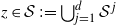 $z\in{\mathcal{S}}\,:\!=\bigcup_{j=1}^d{\mathcal{S}}^{\kern1ptj}$
. We now compute
 $\left\langle {{L}^{0}},L(z) \right\rangle$
,
 $z\in{\mathcal{S}}$
. Let
 $H^0$
and
 $f^0$
be as in the proof of Proposition 5.4. According to Corollary 3.1(ii) with
 $f^1=f^0$
and
 $f^2=f$
,
 $f(t,x,v,w,z)={\mathrm{e}}^{zx}g(t,v,z)$
, and g from (5.9),
 $\vartheta(z)=(zH(z)_t+{\sigma}\rho{\mathrm{e}}^{zX_t}\partial_v g(t,V_t)V_t)S_t^{-1}=\!:\,\widetilde\vartheta(z)$
 $\text{P}\otimes \text{d}\left\langle S,S \right\rangle$
-a.e.,
 $z\in{\mathcal{S}}$
. Thus, the restriction of
 $\widetilde\vartheta$
to
 ${\mathcal{S}}^{\kern1ptj}$
is a predictable function with respect to
 ${\mathcal{S}}^{\kern1ptj}$
,
 $j=1,\ldots,d$
. Furthermore,
 $$\text{d}{{\left\langle {{L}^{0}},L(z) \right\rangle }_{t}}={{\sigma }^{2}}(1-{{\rho }^{2}}){{h}^{\prime }}(\beta (t){{V}_{t}})\beta (t){{\partial }_{v}}g(t,{{V}_{t}},z)V_{t}^{3}{{\text{e}}^{z{{X}_{t}}}}\text{d}t=:\widetilde{K}{{(z)}_{t}}\text{d}t.$$
Since h is twice continuously differentiable and g is twice continuously differentiable in the second variable,  $t\mapsto \widetilde K({\omega},z)_t$
is a continuous function. Because of (5.8) and
 $V_t>0$
, by Theorem 4.3, the assumptions of Theorem 4.1 are satisfied with respect to
 ${\mathcal{S}}^{\kern1ptj}$
, for each
 $j=1,\ldots,d$
, so we have
 $L^{\kern1ptj}_t=\int_{{\mathcal{S}}^{\kern1ptj}}\widetilde L(z){\zeta}^{\kern1ptj}({\mathrm{d}} z)$
, a.s.,
 $t\in[0,T]$
. Since
 $\sup_{z\in{\mathcal{S}}^{\kern1ptj}}{\mathrm{E}}[|\widetilde L(z)_t|^2]<+\infty$
,
 $t\in[0,T]$
,
 $j=1,\ldots,d$
, from Proposition 4.1(iii), the identity
 ${\mathrm{E}}[\,\cdot\,]={\mathrm{E}}[{\mathrm{E}}[\,\cdot\mid V_t]]$
, and (5.12), we obtain the claim.
Proposition 5.6. For  $C=(C^{ij})_{i,j=1,\ldots,d}$
we have
 \[
\begin{split}
C^{ij}=
{\sigma}^2(1-\rho^2)\int_0^T\int_{{\mathcal{S}}^i}\int_{{\mathcal{S}}^{\kern1ptj}}\int_0^{\infty}\Big\{&\partial_vg(t,v,z_1)\partial_vg(t,v,z_2)\times G(t,v,z_1+z_2)v^3f_{V_t}(v)\Big\}\\&\times{\,\mathrm{d}} v\,{\zeta}^{\kern1ptj}({\mathrm{d}} z_2)\,{\zeta}^i({\mathrm{d}} z_1)\,{\,\mathrm{d}} t,
\end{split}
\]
where  $\partial_vg$
is as in (5.10), G(t, v, z) as in Proposition 5.5, and
 $f_{V_t}(v)$
is from (5.7).
Proof. Let  $(\vartheta^{\kern1ptj}, L^{\kern1ptj})$
and
 $(\vartheta(z), L(z))$
be the GKW decompositions with respect to S of
 ${\eta}^{\kern1ptj}$
and of H(z),
 $j=0,\ldots,d$
,
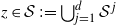 $z\in{\mathcal{S}}\,:\!=\bigcup_{j=1}^d{\mathcal{S}}^{\kern1ptj}$
. By Corollary 3.1(ii) with
 $f^1(t,x,v,w,z)=f(t,x,v,w,z_1)$
,
 $z\in{\mathcal{S}}^ i$
, and
 $f^2(t,x,v,z)=f(t,x,v,w,z_2)$
,
 $z\in{\mathcal{S}}^{\kern1ptj}$
,
 $i,j=1,\ldots,d$
,
 $f(t,x,v,z)={\mathrm{e}}^{zx}g(t,v,z)$
, we get
 $$
\text{d}{{\left\langle L({{z}_{1}}),L({{z}_{2}}) \right\rangle }_{t}}={{\sigma }^{2}}(1-{{\varrho }^{2}}){{\partial }_{v}}g(t,{{V}_{t}},{{z}_{1}}){{\partial }_{v}}g(t,{{V}_{t}},{{z}_{2}}){{\text{e}}^{({{z}_{1}}+{{z}_{2}}){{X}_{t}}}}V_{t}^{3}\text{d}t=:\widetilde{K}({{z}_{1}},{{z}_{2}})\text{d}t.$$
Proof. Let  $(\vartheta^{\kern1ptj}, L^{\kern1ptj})$
and
 $(\vartheta(z), L(z))$
be the GKW decomposition with respect to S of
 ${\eta}^{\kern1ptj}$
and
 $\skew3\widetilde H(z)$
, respectively,
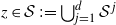 $z\in{\mathcal{S}}\,:\!=\bigcup_{j=1}^d{\mathcal{S}}^{\kern1ptj}$
,
 $j=0,\ldots,d$
. We now compute
 $\left\langle {{L}^{0}},L(z) \right\rangle$
,
 $z\in{\mathcal{S}}$
. Let
 $H^0$
and
 $f^0$
be as in the proof of Proposition 5.1. According to Corollary 3.1 (applied now to the complex-valued square-integrable martingale
 $\skew3\widetilde H(z)$
and to
 $H^0$
) with
 $f^1=f^0$
and
 $f^2=f$
,
 $f(t,x,v,w,z)=\exp(\phi_t(z,0)+\psi_t(z,0)v+zx)$
, we deduce that
 $\vartheta(z)_t=\frac{\skew3\widetilde H(z)_t}{S_t}(z+{\sigma}\rho\psi_{T-t}(z,0))=\!:\,\widetilde\vartheta(z)_t$
 $\text{P}\otimes \text{d}\left\langle S,S \right\rangle$
-a.e.,
 $z\in{\mathcal{S}}$
. Thus, the restriction of
 $\widetilde\vartheta$
to
 ${\mathcal{S}}^{\kern1ptj}$
is a predictable function with respect to
 ${\mathcal{S}}^{\kern1ptj}$
,
 $j=1,\ldots,d$
. Moreover,
 $$\text{d}{{\left\langle {{L}^{0}},L(z) \right\rangle }_{t}}={{\sigma }^{2}}(1-{{\rho }^{2}})\alpha (t){{\psi }_{T-t}}(z,0)\widetilde{H}{{(z)}_{t}}{{V}_{t}}\text{d}t.$$
Proof. We first show claim 1. By assumption (i) of the theorem,  $(t,{\omega},z)\mapsto \skew3\widetilde H({\omega},z)_t$
is optional with respect to
 ${\mathcal{S}}^{\kern1ptj}$
,
 $j=1,\ldots,d$
, and
 $(t,\omega )\mapsto \text{ }\widetilde{H}{{(\omega ,z)}_{t}}$
is càdlàg,
 $z\in{\mathcal{S}}$
. By assumptions (i) and (ii), the function
 $(t,{\omega},z)\mapsto\int_E({\mathrm{e}}^{x_1}-1)W(t,{\omega},x,z)F_t({\omega},{\mathrm{d}} x)$
is predictable with respect to
 ${\mathcal{S}}^{\kern1ptj}$
, for every
 $j=1,\ldots,d$
, the process
 $\xi$
is predictable, and hence the restriction of
 $\widetilde\vartheta$
to
 ${\mathcal{S}}^{\kern1ptj}$
is predictable with respect to
 ${\mathcal{S}}^{\kern1ptj}$
,
 $j=1,\ldots,d$
. Now let
 $(\vartheta(z), L(z))$
be the GKW decomposition of
 $\skew3\widetilde H(z)$
with respect to S, where
 $z\in{\mathcal{S}}$
. From Corollary 3.1, we have
 $\vartheta(z)=\widetilde\vartheta(z)$
 $\text{P}\otimes \text{d}\left\langle S,S \right\rangle$
-a.e. for every
 $z\in{\mathcal{S}}$
. This shows claim 1. To see claim 2, since
 ${{\left\langle L({{z}_{i}}),L({{z}_{j}}) \right\rangle }_{t}}=\int_{0}^{t}{\widetilde{K}{{(\omega ,{{z}_{i}},{{z}_{j}})}_{s}}\text{d}s}$
by Corollary 3.1, we use claim 1 and Theorem 4.2(iii) applied to
 ${\mathcal{S}}^i$
and
 ${\mathcal{S}}^{\kern1ptj}$
.
Proof. The process  ${{(X,V,[X,X])}^{\top }}$
is a locally square-integrable semimartingale whose characteristics are absolutely continuous with respect to the Lebesgue measure. The second differential characteristic c is given by
 $c^{11}=V$
,
 $c^{12}=c^{21}=\rho{\sigma} V$
,
 $c^{22}={\sigma}^2V$
, and
 $c_t^{i3}=0$
,
 $i=1,2,3$
. Since V is a Cox–Ingersoll–Ross process, we have
Proof. Let  $(\vartheta^{\kern1ptj}, L^{\kern1ptj})$
and
 $(\vartheta(z), L(z))$
be the GKW decomposition with respect to S of
 ${\eta}^{\kern1ptj}$
and of
 $\skew3\widetilde H(z)$
, respectively,
 $j=1,\ldots,d$
,
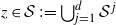 $z\in{\mathcal{S}}\,:\!=\bigcup_{j=1}^d{\mathcal{S}}^{\kern1ptj}$
. By Corollary 3.1(ii) with
 $f^ 1(t,x,v,w,z)=f(t,x,v,w,z_1)$
,
 $z\in{\mathcal{S}}^i$
, and
 $f^2(t,x,v,w,z)=f(t,x,v,w,z_2)$
,
 $z\in{\mathcal{S}}^{\kern1ptj}$
,
 $f(t,x,v,w,z)=\exp(\phi_t(z,0)+\psi_t(z,0)v+zx)$
, we get
 $$
\text{d}{{\left\langle L({{z}_{1}}),L({{z}_{2}}) \right\rangle }_{t}}={{\sigma }^{2}}(1-{{\varrho }^{2}}){{\partial }_{v}}g(t,{{V}_{t}},{{z}_{1}}){{\partial }_{v}}g(t,{{V}_{t}},{{z}_{2}}){{\text{e}}^{({{z}_{1}}+{{z}_{2}}){{X}_{t}}}}V_{t}^{3}\text{d}t=:\widetilde{K}({{z}_{1}},{{z}_{2}})\text{d}t.$$
Since  $\widetilde K$
is
 ${\mathcal{P}}\otimes{\mathcal{B}}({\mathcal{S}}^i)\otimes{\mathcal{B}}({\mathcal{S}}^{\kern1ptj})$
-measurable,
 $t\mapsto\widetilde K({\omega},z_1,z_2)_t$
is continuous, and
 $V_t>0$
, the claim follows from Theorem 4.3 and (5.12).
5.3. An example with jumps
We now consider a special exponential Lévy model with unit jump sizes and compute the quantities A, B, and C for the variance swap.
Let  $N^1$
and
 $N^2$
be independent Poisson processes. Let
 ${\lambda}_i$
be the parameter of
 $N^i$
, that is,
 ${{({{\bar{N}}^{i}})}_{t\in [0,T]}}$
is a martingale,
 $\overline N^i_t\,:\!=N^i_t-{\lambda}_it$
,
 $i=1,2$
. We now introduce the processes
 $M^1_t\,:\!=N^1_t-{\lambda}_1 t({\mathrm{e}}-1)$
and
 $M^2_t\,:\!=N^2_t+{\lambda}_2 t({\mathrm{e}}^{-1}-1)$
and consider the semimartingale
 $X=(X^1,X^2)\,:\!=(X^1_0+M^1-M^2,N^2)$
. Since
 $\Delta N^1\Delta N^2=0$
, the jump measure
 $\mu$
of X is given on
 $E=\{(-1,1),(1,0)\}$
by
 \[
\mu({\omega},{\mathrm{d}} t,{\mathrm{d}} x_1,{\mathrm{d}} x_2)={\mathrm{d}} N^1_t({\omega})\delta_{(1,0)}({\mathrm{d}} x_1,{\mathrm{d}} x_2)+{\mathrm{d}} N^2_t({\omega})\delta_{(-1,1)}({\mathrm{d}} x_1,{\,\mathrm{d}} x_2),
\]
 $\delta_a$
denoting the Dirac measure concentrated at the point a. Hence, the predictable compensator
 $\nu$
of
 $\mu$
is
 \[
\nu({\omega},{\mathrm{d}} t,{\mathrm{d}} x_1,{\mathrm{d}} x_2)= {\lambda}_1\delta_{(1,0)}({\mathrm{d}} x_1,{\mathrm{d}} x_2){\,\mathrm{d}} t+{\lambda}_2\delta_{(-1,1)}({\mathrm{d}} x_1,{\mathrm{d}} x_2){\,\mathrm{d}} t.
\]
The third differential semimartingale characteristic of X is
 \[F_t({\omega},{\mathrm{d}} x)=F({\mathrm{d}} x)={\lambda}_1\delta_{(1,0)}({\mathrm{d}} x_1,{\mathrm{d}} x_2)+{\lambda}_2\delta_{(-1,1)}({\mathrm{d}} x_1,{\mathrm{d}} x_2).\]
We consider the market model  $S={\mathrm{e}}^{M^1-M^2}$
. Then, S is a square-integrable martingale. We now compute the quantities A, B, and C combining Corollary 3.1(i) and Theorem 4.3. The quantity
 $\xi_t$
in Corollary 3.1(i) fulfills
 $\xi_t=\xi=({\mathrm{e}}-1)^2({\lambda}_1+\frac{{\lambda}_2}{{\mathrm{e}}^2})>0$
. For the variance swap we now have
 ${\eta}^0+k=[X^1,X^1]_T=N^1_T+N^2_T$
and
 $k=({\lambda}_1+{\lambda}_2)T$
. We now define
 $f^0(t,x)\,:\!=x^1+2x^2+[{\lambda}_1({\mathrm{e}}-2)+{\lambda}_2({\mathrm{e}}^{-1}-2)] t$
. Then
 $H^0_t={\mathrm{E}}[{\eta}^0\mid{\mathcal{F}}_t]=f^0(t,X)$
holds. Therefore, Corollary 3.1(i) with
 $L^i=L^0$
and
 $W^i=W^0$
,
 $i=1,2$
, where we define
 $W^0\,:\!=f^0(t,x+X_{t-})-f^0(t,X_{t-})=x_1+2x_2$
, yields
 $$A={{\left\langle {{L}^{0}},{{L}^{0}} \right\rangle }_{T}}=\left[ {{\lambda }_{1}}+{{\lambda }_{2}}-\frac{{{({{\lambda }_{1}}-\frac{{{\lambda }_{2}}}{\text{e}})}^{2}}}{{{\lambda }^{1}}+\frac{{{\lambda }^{2}}}{{{\text{e}}^{2}}}} \right]T.$$
We now compute B. Let  ${\mathcal{S}}\,:\!=\bigcup_{j=1}^d{\mathcal{S}}^{\kern1ptj}$
. We observe that
 $X^1$
has exponential moments of every order. Furthermore, since
 $X^1$
has independent increments with respect to the filtration
 ${\mathbb{F}}$
, setting
 $q(z)\,:\!={\lambda}_1({\mathrm{e}}^z-1-z({\mathrm{e}}-1))+{\lambda}_2({\mathrm{e}}^{-z}-1-z({\mathrm{e}}^{-1}-1)),
$
we get
 ${\mathrm{E}}[{\mathrm{e}}^{zX^1_T}\mid{\mathcal{F}}_t]=f(t,X_t,z)=\!:\,\skew3\widetilde H(z)_t$
, where
 $f(t,x,z)\,:\!={\mathrm{e}}^{zx_1+q(z)(T-t)}$
,
 $z\in{\mathbb{C}}$
. Let us consider the GKW decomposition
 $(\vartheta(z),L(z))$
of
 $\skew3\widetilde H(z)$
with respect to S,
 $z\in{\mathcal{S}}$
. We define
 $W(t,x,z)\,:\!=H(z)_{t-}({\mathrm{e}}^{zx_1}-1)$
. Then, by Corollary 3.1(i) applied to
 $L^1=L^0$
and
 $L^2=L(z)$
, with
 $W^1=W^0$
and
 $W^2=W$
, we get
 $\text{d }{{\left\langle {{L}^{0}},L(z) \right\rangle }_{t}}=Q(z)\widetilde{H}{{(z)}_{t-}}\text{d}t$
, where we define
 \[
Q(z)\,:\!=({\mathrm{e}}^z-1)\bigg({\lambda}_1-\frac{{\lambda}_2}{{\mathrm{e}}^ z}-\frac{({\lambda}_1-\frac{{\lambda}_2}{{\mathrm{e}}})({\lambda}_1+\frac{{\lambda}_2}{{\mathrm{e}}^{z+1}})}{{\lambda}_1+\frac{{\lambda}_2}{{\mathrm{e}}^2}}\bigg).\]
Assumptions (ii) of Theorem 4.3 are satisfied, and hence the assumptions of Theorem 4.1 are satisfied. Thus,  $L^{\kern1ptj}_t=\int_{{\mathcal{S}}^{\kern1ptj}}\widetilde L(z)_t{\zeta}^{\kern1ptj}({\mathrm{d}} z)$
, a.s.,
 $t\in[0,T]$
,
 $j=1,\ldots,d$
. Since
 $\skew3\widetilde H(z)_-$
is locally bounded, it is integrable with respect to
 ${\mathrm{Leb.}}$
on [0,T]. So, Proposition 4.1(iii) yields
 $B^{\kern1ptj}=T\int_{{\mathcal{S}}^{\kern1ptj}}\exp(zX_0^1+q(z)T)Q(z){\zeta}^{\kern1ptj}({\mathrm{d}} z)$
.
We now conclude by computing the covariance matrix C. We consider  ${\mathcal{S}}^i$
and
 ${\mathcal{S}}^{\kern1ptj}$
and define
 $f^1(t,x,z)\,:\!=f(t,x,z_1)$
,
 $z_1\in{\mathcal{S}}^ i$
,
 $f^2(t,x,z)\,:\!=f(t,x,z_2)$
,
 $z_2\in{\mathcal{S}}^{\kern1ptj}$
, and
 \[
P(z_1,z_2)\,:\!=({\mathrm{e}}^{z_1}-1)({\mathrm{e}}^ {z_2}-1)\left(\!{\lambda}_1\!+\!\frac{{\lambda}_2}{\exp(z_1+z_2)}-\frac{\left({\lambda}_1+\frac{{\lambda}_2}{\exp({z_1+1})}\right)\left({\lambda}_1+\frac{{\lambda}_2}{\exp({z_2+1})}\right)}{{\lambda}_1+\frac{{\lambda}_2}{{\mathrm{e}}^2}}\!\right).
\]
Then Corollary 3.1(i) yields  $\text{d}{{\left\langle L({{z}_{1}}),L({{z}_{2}}) \right\rangle }_{t}}=P({{z}_{1}},{{z}_{2}})H{{({{z}_{1}})}_{t-}}H{{({{z}_{2}})}_{t-}}\text{d}t$
,
 $z_1\in{\mathcal{S}}^i$
,
 $z_2\in{\mathcal{S}}^{\kern1ptj}$
, and the density is locally bounded. From Theorem 4.3, we get
 \[
\begin{split}
C^{ij}=\int_0^T\int_{{\mathcal{S}}^i}\int_{{\mathcal{S}}^{\kern1ptj}}\Big\{\!&\exp((z_1+z_2)X^1_0+q(z_1+z_2)t+(q(z_1)+q(z_2))(T-t))\\
&\,\times P(z_1,z_2)\Big\}{\zeta}^{\kern1ptj}({\mathrm{d}} z_2){\zeta}^i({\mathrm{d}} z_1){\,\mathrm{d}} t.
\end{split}
\]
Acknowledgements
We acknowledge funding from the German Research Foundation (DFG) under grant ZUK 64 (all authors) and KE 1736/1-1 (MKR, MH). MKR thanks Johannes Muhle-Karbe for early discussions on the idea of ‘variance-optimal semi-static hedging’. We are grateful to the associate editor and to the two referees for their detailed comments which have helped to improve the paper considerably.


