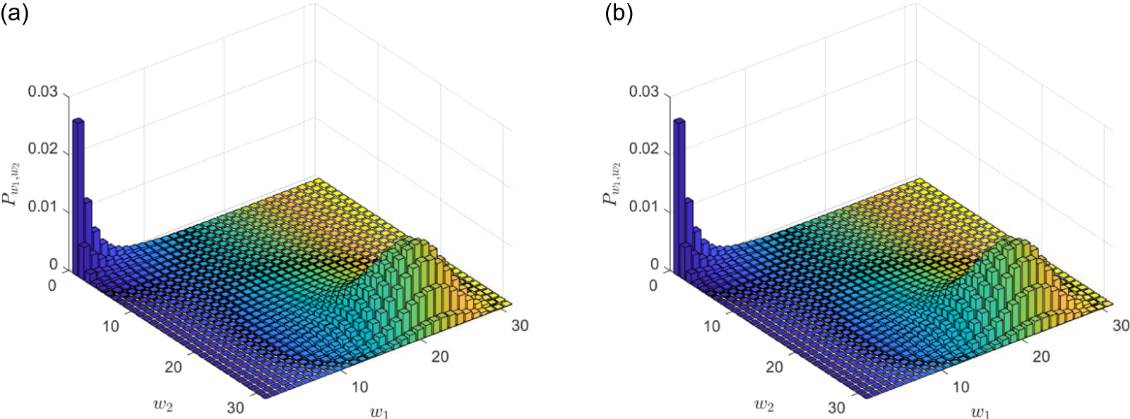
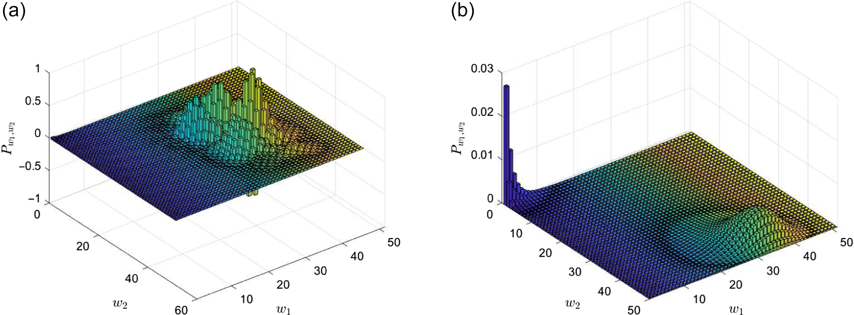
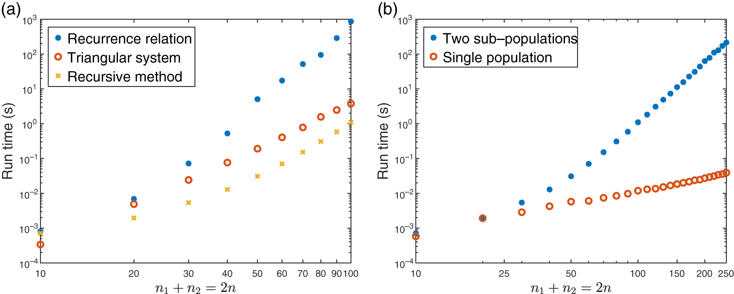
1. Introduction
There is now a considerable body of literature on stochastic SIR (susceptible
 $\to$
infective
 $\to$
removed) epidemics in closed populations. In an SIR epidemic there are three types of individual: susceptibles, infectives, and recovered. If a susceptible is contacted by an infective they also become an infective and remain so for a period of time known as the infectious period, after which they are removed and play no further role in the epidemic. The epidemic eventually ends, since the population is closed. The final size of the epidemic is the number of initial susceptibles who become infected. The sum of the infectious periods of all individuals infected during the epidemic is known as its severity. There have been numerous papers on exact results for the final outcome of stochastic SIR epidemics.
The most-studied continuous-time stochastic SIR epidemic model is the general stochastic epidemic; see e.g. Bailey [Reference Bailey3, Chapter 6]. This assumes that the population is homogeneously mixing, the infectious periods of infectives follow independent exponential random variables, having rate
 $\gamma$
, and contacts between any given infective and any given susceptible occur at the points of independent Poisson processes, each having rate
 $\beta$
. Thus, if there are i infectives and s susceptibles at time t, then new infectives are created at overall rate
 $\beta s i$
and infectives are removed at overall rate
 $\gamma i$
. In Bailey [Reference Bailey2], a two-dimensional linear system of equations is derived, which enables the probability mass function of the final size to be computed. Subsequently, a one-dimensional triangular system of linear equations for this probability mass function was obtained in Whittle [Reference Whittle18]. The assumption of an exponentially distributed infectious period, although mathematically convenient as it leads to a Markov model, is unrealistic for most real-life diseases. In Ball [Reference Ball4], a Wald’s identity for the epidemic process is used to derive a similar triangular system for a model in which the infectious period follows an arbitrary but specified distribution, together with results concerning the severity and extensions to multi-population epidemics. The broader class of collective Reed–Frost epidemic processes was introduced in Picard and Lefèvre [Reference Picard and Lefèvre13] and used to give a unified and extended approach to the above results in terms of Gontcharoff polynomials.
For most real-life epidemics, infectives are not equally infectious throughout their infectious period. This can be modelled by assuming that infectives have independent and identically distributed infectivity profiles,
 $\{I(u)\}=\{I(u)\colon u \ge 0\}$
, where I(u) is the infectiousness of an infective u time units after they were first infected. In a recent paper, Simon [Reference Simon16] considered a model in which infectives behave independently, with the infectivity profile of an infective given by
 $I(u)=\gamma(X(u))$
 $(u\ge 0)$
, where
 $\{X(u)\}$
is a Feller process taking values in a metric space
 $\mathcal{E}$
and
 $\gamma\colon \mathcal{E} \to [0, \infty)$
. It is also assumed that the overall rate that a given infective infects susceptibles at a given time takes the form
 $\beta_s \gamma(x)$
, where s and x are respectively the number of susceptibles and the state of the infective’s Feller process at that time; cf. Clancy [Reference Clancy7], in which the joint distribution of the final size and severity of a standard SIR epidemic under a similar assumption concerning
 $\beta_s$
is derived. (Note that the usual homogeneously mixing assumption implies that
 $\beta_s=s \beta$
, for some
 $\beta>0$
.) In [Reference Simon16], a family of continuous-time martingales associated with the epidemic process is constructed and the optional stopping theorem is used to determine the joint distribution of statistics associated with the final outcome. In particular, a triangular system of linear equations is obtained for the final size distribution. A related discrete-time epidemic process is considered, in which there is a pool of infectives, who are exposed one at a time to the susceptibles, with infected susceptibles being added to the pool. The outcome of a single infective in this process is again determined by using a family of continuous-time martingales. The final outcome of the discrete-time epidemic process is then derived using discrete-time martingales and shown to have the same distribution as that of the original continuous-time epidemic. This is useful in practice since the above-mentioned triangular systems may be numerically unstable for even moderately sized populations (see e.g. House et al. [Reference House, Ross and Sirl9]), whereas, as illustrated in [Reference Simon16], the associated discrete-time epidemic process yields a numerically stable two-dimensional recursive system of equations.
For the special case when
 $\beta_s=s\beta$
, the distribution of the final size of the epidemic can be obtained using [Reference Picard and Lefèvre13], with
 $\int_0^{\infty} I(u) \,{{\mathrm{d}}} u$
playing the same role as the infectious period, and the distribution of more general final outcome statistics can be found using the notion of epidemic general final state random variables (Ball and O’Neill [Reference Ball and O’Neill5]); see the discussion of Ball et al. [Reference Ball, Sirl and Trapman6]. In that special case it is clear by considering the usual random directed graph associated with an SIR epidemic (see e.g. Andersson and Britton [Reference Andersson and Britton1, Chapter 7.1]), that the final outcomes of the continuous-time epidemic and its associated discrete-time epidemic have the same distribution. (Indeed, such an associated discrete-time epidemic is used to analyse the final size of a collective Reed–Frost epidemic in Lefèvre and Utev [Reference Lefèvre and Utev11]; see also Martin-Löf [Reference Martin-Löf12].) In the present paper, we use Sellke-type constructions (see Sellke [Reference Sellke15]) of the continuous-time and associated discrete-time epidemics to give a direct, probabilistic proof that their final outcomes are identically distributed for any choice of
 $\beta_s$
. This leads to proofs of slight generalisations of the results in [Reference Simon16], which hold under more general assumptions concerning the infectivity profile
 $\{I(u)\}$
; all that is required is that its sample paths are almost surely integrable. Moreover, the proofs generalise easily to multipopulation epidemics.
The remainder of the paper is organised as follows. The single-population epidemic is treated in Section 2. The model is defined in Section 2.1 and the main theorem (Theorem 2.1), which gives a set of equations that determines the joint distribution of the final size and a vector of final outcome statistics, is presented. The associated discrete-time epidemic process is described in Section 2.2. The Sellke constructions of the two epidemic processes are given in Section 2.3 and used to show that they have identically distributed final outcomes (Lemma 2.1). Theorem 2.1 is proved in Section 2.1 by proving the corresponding result for the associated discrete-time process. First the outcome of a single infective is determined by exploiting a related death process. Then the discrete-time martingale argument of [Reference Simon16] is used to derive the distribution of the final outcome of the discrete-time epidemic process. Computation of the final outcome distribution is considered in Section 2.5, where an equivalent recurrence relation to that in [Reference Simon16] is derived. The multipopulation epidemic is treated in Section 3, the structure of that section being outlined at its start. Section 3 includes a brief numerical study which investigates the practical usefulness of the discrete-time epidemic process for calculating the final size distribution of a multipopulation epidemic. Finally, some very brief concluding comments are given in Section 4.
2. Single-population epidemics
2.1. Model and final outcome
We consider the following model for the spread of an epidemic in a closed, homogeneously mixing population, which at time
 $t=0$
contains m infectives, who have just become infected, and n susceptibles. Infectives have independent infectivity profiles, each distributed according to a non-negative stochastic process
 $\{I(u)\}$
, where I(u) represents the infectiousness of an infective with infectious age u, i.e. u time units after they were infected. Conditional upon their infectivity profile, an infective makes infectious contacts with susceptibles at the points of an independent Poisson process whose intensity depends on the number of susceptibles present in the population. More precisely, if there are s susceptibles in the population when the infective has infectious age u, then they make contact with susceptibles at overall rate
 $\beta_s I(u)$
. Each contact with susceptibles is with an individual chosen independently and uniformly from the set of susceptibles at that time. Apart from being related through the number of susceptibles, the Poisson processes governing contacts made by infectives are mutually independent. We assume
 $\beta_s>0$
 $(s=1,2,\ldots, n)$
and
 $\beta_s e \beta_{s'}$
for
 $s e s'$
. As mentioned in the Introduction, in [Reference Simon16],
 $I(u)=\gamma(X(u))$
 $(u\ge 0)$
, where
 $\{X(u)\}$
is a Feller process. We make no assumptions concerning the distribution of
 $\{I(u)\}$
, apart from it being integrable and such that there exists a time T, which is almost surely finite, after which no further susceptibles are infected in the epidemic. Note that
 $\{I(u)\}$
may be deterministic and may include an (almost surely finite) latent period before an infected individual is able to make infectious contacts. Denote this model by
 $\mathcal{E}_{n,m}$
. Motivation for and several examples of this type of epidemic model are given in [Reference Simon16].
Let
 ${\boldsymbol{R}}=(R_1, R_2, \ldots, R_p)^{\top}$
, where
 $\top$
denotes transpose, be a vector of p non-negative quantities associated with an infective. One may be their severity
 $A=\int_0^{\infty} I(u) \,{{\mathrm{d}}} u$
. (Note that we allow the possibility that
 $A=\infty$
.) More generally, there may be a cost
 $C=\int_0^{\infty} c(I(u)) \,{{\mathrm{d}}} t$
associated with an infective, where
 $c\colon [0, \infty) \to [0, \infty)$
. Another is the length of the infective’s infectious period
 $T_I=\inf\{v \ge 0\colon I(u)=0 \text{ for all } u >v\}$
. (Note that
 $\mathbb{P}(T_I=\infty)$
may be strictly positive.) In [Reference Simon16],
 $\mathbb{P}(T_I<\infty)=1$
and removals are partitioned into two types: type 1 in which the infective died from the disease and type 2 in which they recover, with the rates of removal of the two types at infectious age u being dependent on X(u), the state of their associated Feller process. This may be included in our framework by letting
 $R_i$
be the indicator function of the removal being of type i
 $(i=1,2)$
.
For
 $t \ge 0$
, let S(t) be the number of susceptibles in the population at time t, so
 $S(0)=n$
. Let
 $S=S(\infty)$
be the number of susceptibles remaining at the end of the epidemic and
 $Z=n-S$
be the size of the epidemic. Let
 $A^F$
be the sum of the severities of all
 $m+Z$
infectives involved in the epidemic and let
 ${\boldsymbol{R}}^F$
be the sum of their associated vector quantities
 ${\boldsymbol{R}}$
. The following theorem, proved in Section 2.4, enables the joint distribution of
 $(S, {\boldsymbol{R}}^F)$
to be determined. For
 $i,j=0,1,\ldots,$
we use the convention that
 $\prod_{l=i}^{i-j}=1$
if
 $j=1$
and 0 if
 $j>1$
. Let
 $\beta_0=0$
and
 $\boldsymbol{\theta}=(\theta_1, \theta_2, \ldots, \theta_p)^{\top}$
.
Theorem 2.1. For
 $k=0,1,\ldots,n$
and
 $\boldsymbol{\theta} \in [0, \infty)^p$
,
 \begin{equation*}\mathbb{E}\Biggl[\Biggl(\prod_{l=k+1}^S \dfrac{\beta_l}{\beta_l-\beta_k}\Biggr){\exp}{(\!-\boldsymbol{\theta}}^{\top} {\boldsymbol{R}}^F)q_k(\boldsymbol{\theta})^S\Biggr]=q_k(\boldsymbol{\theta})^{n+m}\prod_{l=k+1}^n \dfrac{\beta_l}{\beta_l-\beta_k},\end{equation*}
where
 \begin{equation}q_k(\boldsymbol{\theta})=\mathbb{E}[{\exp}{(\!-(\boldsymbol{\theta}}^{\top} {\boldsymbol{R}}+\beta_k A))].\end{equation}
2.2. Weiss and artificial-time epidemics
In the carrier-borne epidemic model of Weiss [Reference Weiss17], only the initial infectives are able to create new infectives. In the present setting, consider a model with initially one infective, having infectivity profile
 $\{\tilde{I}(u)\}$
and associated vector quantity
 $\tilde{{\boldsymbol{R}}}$
, and s susceptibles, where
 $0 \le s \le n$
. The dynamics of the epidemic are the same as those of
 $\mathcal{E}_{n,m}$
, except that contacted susceptibles do not make further infectious contacts. Let
 $\tilde{N}(s)$
denote the number of susceptibles infected by the infective. Denote this model by
 $\mathcal{E}_s^{m Weiss}$
.
We now consider an epidemic with initially m infectives and n susceptibles. The infectives are placed in a pool and are considered one at a time. For each infective considered, a Weiss epidemic takes place among the remaining susceptibles; any susceptible that is infected by the Weiss epidemic is added to the pool of infectives. Let
 $\tilde{S}_0=n$
,
 $\tilde{A}^C_0=0$
, and
 $\tilde{{\boldsymbol{R}}}^C_0=\boldsymbol{0}^{\top}$
. (Throughout the paper,
 $\boldsymbol{0}$
denotes a row vector of zeros whose dimension, in the present case p, is apparent from the context.) For
 $\tau=1,2,\ldots,$
let
 $\{\tilde{I}_{\tau}(u)\}$
and
 $\tilde{{\boldsymbol{R}}}_{\tau}$
denote the infectivity profile and vector quantity of the
 $\tau$
th infective considered. Let
 $\tilde{A}_{\tau}=\int_0^{\infty} \tilde{I}_{\tau}(u) \,{{\mathrm{d}}} u$
be their severity and let
 $\tilde{N}_{\tau}$
denote the number of susceptibles that they infect. Let
 $\tilde{S}_{\tau}$
be the number of susceptibles remaining after
 ${\tau}$
infectives have been considered, and let
 $\tilde{A}_{\tau}^C$
and
 $\tilde{{\boldsymbol{R}}}_{\tau}^C$
be the (cumulative) sums of the severities and vector quantities of the first
 $\tau$
infectives considered. Thus, for
 $\tau=0,1,\ldots,$
 \begin{align*}\tilde{S}_{\tau+1}=\tilde{S}_{\tau}-\tilde{N}_{\tau+1},\quad \tilde{A}_{\tau+1}^C=\tilde{A}_{\tau}^C+\tilde{A}_{\tau+1} \quad\text{and}\quad \tilde{{\boldsymbol{R}}}_{\tau+1}^C=\tilde{{\boldsymbol{R}}}_{\tau}^C+\tilde{{\boldsymbol{R}}}_{\tau+1}. \end{align*}
The process stops when the pool of infectives becomes empty after an infective has been considered. Let
 $\tilde{\mathcal{T}}$
be the number of infectives considered when the process stops. Then
 \begin{equation}\tilde{\mathcal{T}}=\inf\{\tau \ge 0\colon \tau+\tilde{S}_{\tau}=m+n\}.\end{equation}
The size of the epidemic is given by
 $\tilde{Z}=\tilde{\mathcal{T}}-m$
, and the sums of the severities and vector quantities of all infectives involved in the epidemic are given by
 $\tilde{A}^F=\tilde{A}^C_{\tilde{\mathcal{T}}}$
and
 $\tilde{{\boldsymbol{R}}}^F=\tilde{{\boldsymbol{R}}}^C_{\tilde{\mathcal{T}}}$
, respectively. Denote this epidemic process by
 $\tilde{\mathcal{E}}_{n,m}$
. Following [Reference Simon16], we call it an artificial-time epidemic process.
2.3. Sellke construction
We now give Sellke-type constructions (see [Reference Sellke15]) of the epidemics
 $\mathcal{E}_{n,m}$
and
 $\tilde{\mathcal{E}}_{n,m}$
, which we use to show that if
 $(\{I(u)\},{\boldsymbol{R}})\stackrel{\mathrm{D}}{=}(\{\tilde{I}(u)\},\tilde{{\boldsymbol{R}}})$
then
 $(S,{\boldsymbol{R}}^F) \stackrel{\mathrm{D}}{=} (\tilde{S},\tilde{{\boldsymbol{R}}}^F)$
, where
 $\stackrel{\mathrm{D}}{=}$
denotes equal in distribution.
For the construction of
 $\mathcal{E}_{n,m}$
, let
 $L_1,L_2,\ldots, L_n$
be independent and identically distributed (i.i.d.)
 ${m Exp}(1)$
(unit-mean exponential) random variables. Let
 $(\{I_i(u)\},{\boldsymbol{R}}_i)$
 $(i=-(m-1), -(m-2), \ldots, n)$
be an independent set of i.i.d. random quantities, each distributed as
 $(\{I(u)\},{\boldsymbol{R}})$
. Label the initial infectives
 $-(m-1), -(m-2), \ldots, 0$
and the initial susceptibles
 $1,2,\ldots, n$
. For
 $t \ge 0$
, let S(t) be the number of susceptibles at time t, so
 $S(0)=n$
. For
 $i=-(m-1), -(m-2), \ldots, 0$
, the initial infective i has infectivity profile and vector quantity
 $(\{I_i(u)\},{\boldsymbol{R}}_i)$
. For
 $i=1,2,\ldots, n$
, the ith susceptible to be infected by the epidemic (if at least i are infected) has infectivity profile and vector quantity
 $(\{I_i(u)\},{\boldsymbol{R}}_i)$
. Let
 $t_i=0$
 $(i=-(m-1), -(m-2), \ldots, 0)$
and for
 $i=1,2,\ldots, n$
, let
 $t_i$
be the time of the ith infection if at least i infections occur, with
 $t_i=\infty$
otherwise. For
 $t \ge 0$
, let
 \begin{align*}V(t)=\int_0^t \sum_{i=-(m-1)}^n \bar{\beta}_{S(u)} I_i(u-t_i) \,{{\mathrm{d}}} u, \end{align*}
where
 $I_i(v)=0$
if
 $v<0$
and
 $\bar{\beta}_s=s^{-1}\beta_s$
, with
 $\bar{\beta}_0=0$
. Note that V(t) is the cumulative infectious pressure exerted on each susceptible by time t. (Provided
 $S(u)>0$
, an infective, with infective profile
 $\{I(u')\}$
, having infectious age a at time u, exerts infectious pressure on susceptibles as a whole at rate
 $\beta_{S(u)}I(a)$
and hence on each susceptible at rate
 $\beta_{S(u)}I(a)/S(u)=\bar{\beta}_{S(u)}I(a)$
.) For
 $i=1,2,\ldots, n$
, individual i becomes infected when V(t) reaches
 $L_i$
. It is seen easily that this yields a realisation of
 $\mathcal{E}_{n,m}$
. Clearly, the infectivity profiles and vector quantities of the infectives have the correct distribution, and the lack-of-memory property of the exponential distribution ensures that the infection process is modelled correctly.
Let
 $L_{(1)}, L_{(2)}, \ldots, L_{(n)}$
be the order statistics of
 $L_1,L_2,\ldots, L_n$
and
 $L_{(0)}=0$
. For
 $i=-(m-1), -(m-2), \ldots, n$
, let
 $A_i=\int_0^{\infty} I_i(u)\,{{\mathrm{d}}} u$
. Recall that Z is the size of the epidemic
 $\mathcal{E}_{n,m}$
. Note that
 \begin{align*}Z \ge 1 \iff L_{(1)}\le \bar{\beta}_n \sum_{i=-(m-1)}^0 A_i \iff \sum_{i=-(m-1)}^0 A_i \ge \bar{\beta}_n^{-1} L_{(1)}, \end{align*}
and, for
 $k=2,3,\ldots,n$
, if
 $Z \ge k-1$
then
 \begin{align*}Z \ge k &\iff L_{(k)}-L_{(k-1)} \le \bar{\beta}_{n+1-k}\Biggl[\sum_{i=-(m-1)}^{k-1} A_i -\sum_{j=1}^{k-1} \bar{\beta}_{n+1-j}^{-1}(L_{(j)}-L_{(j-1)})\Biggr]\\[3pt]&\iff \sum_{i=-(m-1)}^{k-1} A_i \ge r_k=\sum_{j=1}^k \bar{\beta}_{n+1-j}^{-1}(L_{(j)}-L_{(j-1)}).\end{align*}
Define
 $f_L\colon [0, r_n] \to [0, L_{(n)}]$
by linear interpolation between
 $(0,0), (r_1, L_{(1)}), \ldots, (r_n, L_{(n)})$
and note that
 $f_L$
is almost surely bijective. Then
 \begin{equation}Z=\inf\Biggl\{k \ge 0\colon \sum_{i=-(m-1)}^k A_i < f_L^{-1}(L_{(k+1)})\Biggr\},\end{equation}
where
 $f_L^{-1}(L_{(n+1)})=\infty$
, and
 \begin{equation}(A^F, {\boldsymbol{R}}^F)=\sum_{i=-(m-1)}^Z (A_i, {\boldsymbol{R}}_i).\end{equation}
Turning to the construction of
 $\tilde{\mathcal{E}}_{n,m}$
, let
 $L_1, L_2, \ldots, L_n$
be as above and let
 $(\{\tilde{I}_i(u)\},\tilde{{\boldsymbol{R}}}_i)$
 $(i=1,2,\ldots,m+n)$
be an independent set of i.i.d. random quantities, each distributed as
 $(\{\tilde{I}(u)\},\tilde{{\boldsymbol{R}}})$
. For
 $i=1,2,\ldots, m+n$
, let
 $\tilde{A}_i=\int_0^{\infty} \tilde{I}_i(u)\,{{\mathrm{d}}} u$
. The epidemic
 $\tilde{\mathcal{E}}_{n,m}$
is constructed as follows. Let
 $\tilde{S}_0=n$
. The number of susceptibles contacted by the first infective is
 $\tilde{N}_1=\inf\{l \ge 0\colon \tilde{A}_1< f_L^{-1}(L_{(l+1)})\}$
and
 $\tilde{S}_1=n-\tilde{N}_1$
. If
 $\tilde{S}_1=0$
, then
 $(\tilde{S}_{\tau}, \tilde{N}_{\tau})=(0,0)$
for
 $\tau=2,3,\ldots.$
Otherwise, to determine
 $\tilde{N}_2$
, the number of susceptibles contacted by the second infective, for
 $i>\tilde{N}_1$
, let
 ${L}_{(i)}'= {L}_{(i)}-f_L(\tilde{A}_1)$
. Note that, conditional upon
 $f_L(\tilde{A}_1)$
, the lack-of-memory property of the exponential distribution implies that
 ${L}_{(i)}'$
 $(i=\tilde{N}_1+1, \tilde{N}_1+2,\ldots, n)$
are distributed as the order statistics of
 $\tilde{S}_1$
i.i.d.
 ${m Exp}(1)$
random variables that are independent of
 $f_L(\tilde{A}_1)$
. We now use
 ${L}_{(i)}'$
 $(i=\tilde{N}_1+1, \tilde{N}_1+2,\ldots, n)$
to determine
 $\tilde{N}_2$
by exposing the susceptibles with these tolerances to
 $\tilde{A}_2$
units of infectious pressure. Observe that
 $\tilde{N}_1+\tilde{N}_2=\inf\{l \ge 0 \colon \tilde{A}_1+\tilde{A}_2 < f_L^{-1}(L_{(l+1)})\}$
and
 $\tilde{S}_2=n-\tilde{N}_1+\tilde{N}_2$
. The process is continued in the obvious fashion, yielding
 \begin{align*}\tilde{S}_{\tau} = n-\inf\Biggl\{l \ge 0 \colon \sum_{i=1}^l \tilde{A}_i < f_L^{-1}(L_{(l+1)})\Biggr\} \quad (\tau=1,2,\ldots). \end{align*}
Recalling (2.2),
 \begin{align*}\tilde{\mathcal{T}}=\inf\{\tau \ge 0\colon \tau+\tilde{S}_{\tau}=m+n\}=\inf\{k \ge 0\colon \tilde{N}_1+\tilde{N}_2+\cdots+\tilde{N}_{m+k}=k\}. \end{align*}
Thus
 \begin{align}\tilde{Z}=n-\tilde{S}_{\mathcal{T}}&=\inf\{k \ge 0\colon \tilde{N}_1+\tilde{N}_2+\cdots+\tilde{N}_{m+k}=k\} onumber \\[3pt]&=\inf\Biggl\{k \ge 0\colon \sum_{i=1}^{m+k}\tilde{A}_i < f_L^{-1}(L_{(k+1)})\Biggr\}\end{align}
and
 \begin{equation}(\tilde{A}^F, \tilde{{\boldsymbol{R}}}^F)=\sum_{i=1}^{m+\tilde{Z}} (\tilde{A}_i, \tilde{{\boldsymbol{R}}}_i).\end{equation}
Lemma 2.1. If
 $(\{I(u)\}, {\boldsymbol{R}}) \stackrel{\mathrm{D}}{=} (\{\tilde{I}(u)\}, \tilde{{\boldsymbol{R}}})$
, then
 $(Z, {\boldsymbol{R}}^F) \stackrel{\mathrm{D}}{=} (\tilde{Z}, \tilde{{\boldsymbol{R}}}^F)$
.
Proof. Couple the Sellke constructions of
 $\mathcal{E}_{n,m}$
and
 $\tilde{\mathcal{E}}_{n,m}$
by using the same
 $L_1, L_2, \ldots,L_n$
and setting
 $(\{\tilde{I}_i(u)\},\tilde{{\boldsymbol{R}}}_i)=(\{I_{i-m}(u)\}, {\boldsymbol{R}}_{i-m})$
 $(i=1,2,\ldots,m+n)$
. It follows immediately from (2.3) and (2.5) that
 $Z=\tilde{Z}$
, and then from (2.4) and (2.6) that
 ${\boldsymbol{R}}^F=\tilde{{\boldsymbol{R}}}^F$
.
2.4. Proof of Theorem 2.1
We prove Theorem 2.1 by showing that if
 $(\{I(u)\}, {\boldsymbol{R}}) \stackrel{\mathrm{D}}{=} (\{\tilde{I}(u)\}, \tilde{{\boldsymbol{R}}})$
, then the corresponding result holds for the epidemic
 $\tilde{\mathcal{E}}_{n,m}$
(see Lemma 2.4 below). We consider first the Weiss epidemic
 $\mathcal{E}_s^{m Weiss}$
. We first prove a lemma concerning death processes.
Lemma 2.2. Let
 $\{D(t)\colon t \ge 0\}$
be a death process, with
 $D(0)=s \in\{0,1,\ldots,n\}$
and overall death rate
 $\beta_i$
when
 $D(t)=i$
, where
 $\beta_0=0$
and
 $\beta_i e \beta_j$
when
 $i e j$
. For
 $k=0,1,\ldots, n$
,
 \begin{align*}\mathbb{E}\Biggl[\prod_{l=k+1}^{D(t)} \dfrac{\beta_l}{\beta_l-\beta_k} \Biggr]={\exp}{(\!-\beta_k t)}\prod_{l=k+1}^s \dfrac{\beta_l}{\beta_l-\beta_k} \quad\textit{for all $ t \ge 0$.} \end{align*}
Proof. For
 $i,k \in \{0,1,\ldots,n\}$
, let
 \begin{align*}\theta_{k,i}=\prod_{l=k+1}^i \dfrac{\beta_l}{\beta_l-\beta_k}. \end{align*}
It is easily verified that
 \begin{equation}\beta_i(\theta_{k, i-1}-\theta_{k,i})=-\beta_k \theta_{k,i}\quad (i,k\in\{0,1,\ldots,n\}).\end{equation}
For
 $s,k \in \{0,1,\ldots,n\}$
, let
 $g_{s,k}(t)=\mathbb{E}[\theta_{k, D(t)}\mid D(0)=s]$
 $(t \ge 0)$
. For any
 $t \ge 0$
and
 $h>0$
,
 \begin{align*}g_{s,k}(t+h)&=\mathbb{E}\bigl[\theta_{k, D(t+h)}\mid D(0)=s\bigr]\\[3pt]&=\mathbb{E}_{D(t)\mid D(0)=s}\bigl[\mathbb{E}\bigl[\theta_{k, D(t+h)}\mid D(t)\bigr]\bigr]\\[3pt]&=\mathbb{E}_{D(t)\mid D(0)=s}\bigl[\theta_{k, D(t)}+h\beta_{D(t)}(\theta_{k, D(t)-1}-\theta_{k, D(t)})\bigr]+{{\mathrm{o}}}(h)\\[3pt]&=\mathbb{E}_{D(t)\mid D(0)=s}\bigl[\theta_{k, D(t)}-h\beta_k \theta_{k, D(t)}\bigr]+{{\mathrm{o}}}(h),\end{align*}
using (2.7). Hence
 \begin{align*}g_{s,k}(t+h)=g_{s,k}(t)-h\beta_k g_{s,k}(t)+{{\mathrm{o}}}(h), \end{align*}
so, with
 ${g{\prime}}_{s,k}$
denoting the right-derivative of
 $g_{s,k}$
,
 \begin{align*}{g{\prime}}_{s,k}(t)=-\beta_k g_{s,k}(t). \end{align*}
Thus
 $g_{s,k}(t)={\exp}(\!-\beta_k t) g_{s,k}(0)={\exp}{(\!-{\beta}_k t)}\theta_{k,s}$
and the lemma follows.
Armed with Lemma 2.2, it is straightforward to prove the following result concerning the final outcome of the epidemic
 $\mathcal{E}_s^{m Weiss}$
.
Lemma 2.3. Consider the epidemic
 $\mathcal{E}_s^{m Weiss}$
and suppose that
 $(\{\tilde{I}(u)\}, \tilde{{\boldsymbol{R}}}) \stackrel{\mathrm{D}}{=} (\{I(u)\}, {\boldsymbol{R}})$
. Then, for
 $k, s \in \{0,1,\ldots,n\}$
and
 $\boldsymbol{\theta} \in [0, \infty)^p$
,
 \begin{align*}\mathbb{E}\Biggl[\Biggl(\prod_{l=k+1}^{s-\tilde{N}(s)}\dfrac{\beta_l}{\beta_l-\beta_k}\Biggr){\exp}{(\!-\boldsymbol{\theta}}^{\top} \tilde{{\boldsymbol{R}}})\Biggr]=q_k(\boldsymbol{\theta})\prod_{l=k+1}^s \dfrac{\beta_l}{\beta_l-\beta_k}, \end{align*}
where
 $q_k(\boldsymbol{\theta})$
is given by (2.1).
Proof. For
 $k, s \in \{0,1,\ldots,n\}$
and
 $\boldsymbol{\theta} \in [0, \infty)^p$
,
 \begin{align*}\mathbb{E}\Biggl[\Biggl(\prod_{l=k+1}^{s-\tilde{N}(s)}\dfrac{\beta_l}{\beta_l-\beta_k}\Biggr){\exp}(\!-\boldsymbol{\theta}^{\top} \tilde{{\boldsymbol{R}}})\Biggr]&=\mathbb{E}\Biggl[\mathbb{E}\Biggl[\Biggl(\prod_{l=k+1}^{s-\tilde{N}(s)}\dfrac{\beta_l}{\beta_l-\beta_k}\Biggr){\exp}(\!-\boldsymbol{\theta}^{\top} \tilde{{\boldsymbol{R}}})\biggm|\tilde{A}, \tilde{{\boldsymbol{R}}}\Biggr]\Biggr]\\[3pt]&=\mathbb{E}\Biggl[{\exp}(\!-\boldsymbol{\theta}^{\top} \tilde{{\boldsymbol{R}}})\mathbb{E}\Biggl[\Biggl(\prod_{l=k+1}^{s-\tilde{N}(s)}\dfrac{\beta_l}{\beta_l-\beta_k}\Biggr)\biggm|\tilde{A}\Biggr]\Biggr]\\[3pt]&=\mathbb{E}\Biggl[{\exp}(\!-\boldsymbol{\theta}^{\top} \tilde{{\boldsymbol{R}}}){\exp}(\!-\beta_k \tilde{A})\Biggl(\prod_{l=k+1}^{s}\dfrac{\beta_l}{\beta_l-\beta_k}\Biggr)\Biggr]\\[3pt]&=q_k(\boldsymbol{\theta})\prod_{l=k+1}^s \dfrac{\beta_l}{\beta_l-\beta_k},\end{align*}
where in the third equality we have used Lemma 2.2.
Finally, we consider the artificial-time epidemic process
 $\tilde{\mathcal{E}}_{n,m}$
. The proof of the next lemma closely follows that of Proposition 4.2 of [Reference Simon16].
Lemma 2.4. Consider the epidemic
 $\tilde{\mathcal{E}}_{n,m}$
and suppose that
 $(\{\tilde{I}(u)\}, \tilde{{\boldsymbol{R}}}) \stackrel{\mathrm{D}}{=} (\{I(u)\}, {\boldsymbol{R}})$
. Then, for
 $k \in \{0,1,\ldots,n\}$
and
 $\boldsymbol{\theta} \in [0, \infty)^p$
,
 \begin{equation}\mathbb{E}\Biggl[\Biggl(\prod_{l=k+1}^{\tilde{S}_{\tilde{\mathcal{T}}}} \dfrac{\beta_l}{\beta_l-\beta_k}\Biggr){\exp}(\!-\boldsymbol{\theta}^{\top} \tilde{{\boldsymbol{R}}}^F)q_k(\boldsymbol{\theta})^{\tilde{S}_{\tilde{\mathcal{T}}}}\Biggr]=q_k(\boldsymbol{\theta})^{n+m}\prod_{l=k+1}^n \dfrac{\beta_l}{\beta_l-\beta_k},\end{equation}
where
 $q_k(\boldsymbol{\theta})$
is given by (2.1).
Proof. For
 $\tau=0,1,\ldots,$
let
 $\mathcal{H}_{\tau}=\mathcal{F}\{(\tilde{S}_l, \tilde{A}_l, \tilde{{\boldsymbol{R}}}_l)\colon l=0,1,\ldots,\tau\}$
. Fix
 $k, \boldsymbol{\theta}$
and let
 \begin{align*}\tilde{W}_{\tau}=\Biggl(\prod_{l=k+1}^{\tilde{S}_{\tau}} \dfrac{\beta_l}{\beta_l-\beta_k}\Biggr){\exp}(\!-\boldsymbol{\theta}^{\top} \tilde{{\boldsymbol{R}}}_{\tau}^C)q_k(\boldsymbol{\theta})^{-\tau} \quad (\tau=0,1,\ldots). \end{align*}
We show that
 $\{\tilde{W}_{\tau}\colon \tau=0,1,\ldots\}$
is a martingale with respect to
 $\{\mathcal{H}_{\tau}\colon \tau=0,1,\ldots\}$
and then apply the optional stopping theorem, with the stopping time
 $\tilde{\mathcal{T}}$
, to prove (2.8).
For
 $\tau=0,1,\ldots,$
 \begin{align*}\mathbb{E}[\tilde{W}_{\tau+1}\mid \mathcal{H}_\tau]&=\mathbb{E}\Biggl[\Biggl(\prod_{l=k+1}^{\tilde{S}_{\tau+1}} \dfrac{\beta_l}{\beta_l-\beta_k}\Biggr){\exp}(\!-\boldsymbol{\theta}^{\top} \tilde{{\boldsymbol{R}}}_{\tau+1}^C)q_k(\boldsymbol{\theta})^{-(\tau+1)}\biggm|\mathcal{H}_\tau\Biggr]\\[3pt]&={\exp}(\!-\boldsymbol{\theta}^{\top} \tilde{{\boldsymbol{R}}}_{\tau}^C)q_k(\boldsymbol{\theta})^{-(\tau+1)}\mathbb{E}\Biggl[\Biggl(\prod_{l=k+1}^{\tilde{S}_{\tau+1}} \dfrac{\beta_l}{\beta_l-\beta_k}\Biggr){\exp}(\!-\boldsymbol{\theta}^{\top} \tilde{{\boldsymbol{R}}}_{\tau+1})\biggm|\tilde{S}_{\tau}\Biggr]\\[3pt]&={\exp}(\!-\boldsymbol{\theta}^{\top} \tilde{{\boldsymbol{R}}}_{\tau}^C)q_k(\boldsymbol{\theta})^{-(\tau+1)}\Biggl(\prod_{l=k+1}^{\tilde{S}_{\tau}} \dfrac{\beta_l}{\beta_l-\beta_k}\Biggr)q_k(\boldsymbol{\theta}) \quad (\text{using Lemma }{2.3})\\[3pt]&=\tilde{W}_{\tau}.\end{align*}
Hence
 $\{\tilde{W}_{\tau}\colon \tau=0,1,\ldots\}$
is a martingale.
Now
 $\tilde{\mathcal{T}}$
is a stopping time with respect to
 $\{\mathcal{H}_{\tau}\colon \tau=0,1,\ldots\}$
and
 $\mathbb{P}(\tilde{\mathcal{T}} \le m+n)=1$
, so
 $\mathbb{E}[\tilde{W}_{\tilde{\mathcal{T}}}]=\mathbb{E}[\tilde{W}_0]$
by the optional stopping theorem. Hence
 \begin{align*}\mathbb{E}\Biggl[\Biggl(\prod_{l=k+1}^{\tilde{S}_{\tilde{\mathcal{T}}}} \dfrac{\beta_l}{\beta_l-\beta_k}\Biggr){\exp}(\!-\boldsymbol{\theta}^{\top} \tilde{{\boldsymbol{R}}}_{\tilde{\mathcal{T}}}^C)q_k(\boldsymbol{\theta})^{-\tilde{\mathcal{T}}}\Biggr]=\prod_{l=k+1}^n \dfrac{\beta_l}{\beta_l-\beta_k}, \end{align*}
and (2.8) follows on noting that
 $\tilde{\mathcal{T}}=m+n-\tilde{S}_{\tilde{\mathcal{T}}}$
(see (2.2)) and
 $\tilde{{\boldsymbol{R}}}^F=\tilde{{\boldsymbol{R}}}_{\tilde{\mathcal{T}}}^C$
.
2.5. Computation
Consider the epidemic
 $\mathcal{E}_{n,m}$
. Fix
 $\boldsymbol{\theta} \in [0, \infty)^p$
and
 $g\colon \{0,1,\ldots,n\} \to \mathbb{R}$
, and let
 \begin{align*}G_{n,m}(\boldsymbol{\theta})=\mathbb{E}[g(S){\exp}(\!-\boldsymbol{\theta}^{\top}{\boldsymbol{R}}^F)]. \end{align*}
Note that Theorem 2.1 yields a triangular system of linear equations for
 $\mathbb{E}[1_{\{S=i\}} {\exp}(\!-\boldsymbol{\theta}^{\top}{\boldsymbol{R}}^F)]$
 $(i=0,1,\ldots, n)$
, which in principle can be solved numerically and hence yield
 $G_{n,m}(\boldsymbol{\theta})$
. Alternatively, Corollary 3.2 of Lefèvre and Picard [Reference Lefèvre and Picard10] can be used to express
 $G_{n,m}(\boldsymbol{\theta})$
in terms of Abel–Gontcharoff pseudopolynomials
 $G_0, G_1, \ldots, G_n$
, which are defined recursively via a triangular system of linear equations (see [Reference Clancy7, Theorem 2 (iv)]). However, in practice, these triangular systems may be numerically unstable, even for moderately sized n. Thus, following [Reference Simon16], we show how
 $G_{n,m}(\boldsymbol{\theta})$
can be calculated using the epidemic process
 $\tilde{\mathcal{E}}_{n,m}$
and Lemma 2.1.
We first prove a lemma concerning the outcome of the epidemic
 $\mathcal{E}_s^{m Weiss}$
. The lemma is analogous to Proposition 4.1 of [Reference Simon16], though the proof here is more direct.
Lemma 2.5. Consider the epidemic
 $\mathcal{E}_s^{m Weiss}$
and suppose that
 $(\{\tilde{I}(u)\}, \tilde{{\boldsymbol{R}}}) \stackrel{\mathrm{D}}{=} (\{I(u)\}, {\boldsymbol{R}})$
. Then, for
 $s \in \{0,1,\ldots,n\}$
,
 $l \in \{0,1,\ldots,s\}$
and
 $\boldsymbol{\theta} \in [0, \infty)^p$
,
 \begin{align*}\mathbb{E}\bigl[1_{\{s-\tilde{N}(s)=l\}}{\exp}(\!-\boldsymbol{\theta}^{\top}\tilde{{\boldsymbol{R}}})\bigr]=\sum_{k=l}^s Q_s(l,k) q_k(\boldsymbol{\theta}), \end{align*}
where

Proof. Let
 $\{D(t)\colon t \ge 0\}$
be as in Lemma 2.2. For
 $l=s, s-1, \ldots, 0$
, let
 $X_l$
denote the sojourn time of
 $\{D(t)\colon t \ge 0\}$
in state l, so
 $X_0=\infty$
. Then, for
 $t \ge 0$
and
 $l=s,s-1, \ldots, 0$
,

see e.g. Feller [Reference Feller8, page 40]. (Note that
 $X_s+X_{s-1}+\cdots+X_l$
has a hypoexponential distribution.) Hence, for
 $l=s, s-1, \ldots, 0$
,
 \begin{equation}\mathbb{P}(D(t)=l)=\mathbb{P}(D(t) \ge l)-\mathbb{P}(D(t) \ge l+1)=\sum_{k=l}^s Q_s(l,k) {\exp}(\!-\beta_k t).\end{equation}
Turning to the epidemic
 $\mathcal{E}_s^{m Weiss}$
, for
 $s \in \{0,1,\ldots,n\}$
,
 $l \in \{0,1,\ldots,s\}$
and
 $\boldsymbol{\theta} \in [0, \infty)^p$
,

Now consider the epidemic process
 $\tilde{\mathcal{E}}_{n,m}$
. Fix
 $\boldsymbol{\theta} \in [0, \infty)^p$
and
 $g\colon \{0,1,\ldots,n\} \to \mathbb{R}$
, and let
 \begin{align*}\tilde{G}_{n,m}(\boldsymbol{\theta})=\mathbb{E}\bigl[g(n-\tilde{Z})\,{\exp}\bigl(\!-\boldsymbol{\theta}^{\top}\tilde{{\boldsymbol{R}}}^F\bigr)\bigr]. \end{align*}
By conditioning on
 $(\tilde{N_1}, \tilde{{\boldsymbol{R}}}_1)$
and using the strong Markov property, it is straightforward to obtain the following recurrence relation for
 $\tilde{G}_{n,m}(\boldsymbol{\theta})$
 $((n,m) \in \mathbb{Z}_+^2)$
. The proof parallels that of Proposition 4.3 of [Reference Simon16], and is omitted.
Proposition 2.1. Suppose that
 $(\{\tilde{I}(u)\}, \tilde{{\boldsymbol{R}}}) \stackrel{\mathrm{D}}{=} (\{I(u)\}, {\boldsymbol{R}})$
. Then, for fixed
 $\boldsymbol{\theta} \in [0, \infty)^p$
and fixed
 $g\colon \{0,1,\ldots,n\} \to \mathbb{R}$
,
 \begin{align*}\tilde{G}_{n,m}(\boldsymbol{\theta})=\begin{cases}\displaystyle \sum_{l=0}^n \sum_{k=l}^n Q_n(l,k) q_k(\boldsymbol{\theta}) \tilde{G}_{l,m-1+n-l} & \textit{if $ m>0$,}\\[9pt]g(n)& \textit{if $ m=0$.}\end{cases} \\[-30pt] onumber \end{align*}
As illustrated in [Reference Simon16], Proposition 2.1 provides a numerically more stable method than Theorem 2.1 for computing final outcome properties of an SIR epidemic.
3. Multipopulation epidemics
We now extend the above theory to multipopulation epidemics. The proofs are a natural extension of those used for single-population epidemics, though the material is presented in a slightly different order; the proofs of results for the Weiss and artificial-time epidemics are given in the sections where those epidemics are described. The multipopulation epidemic model and the main result (Theorem 3.1) are described in Section 3.1. The Weiss and artificial-time epidemics are covered in Sections 3.2 and 3.3, respectively, with computational aspects treated in Section 3.4. The Sellke constructions of the continuous-time and artificial-time epidemics are given in Section 3.5, together with a proof that they yield the same final outcome distribution (Lemma 3.4). Finally, some numerical examples are given in Section 3.6.
3.1. Model and final outcome
We assume that the population is split into J sub-populations, labelled
 $1,2,\ldots, J$
, with individuals being typed according to the sub-population to which they belong. Let
 $\mathcal{J}=\{1,2,\ldots,J\}$
. For
 $i \in \mathcal{J}$
, sub-population i initially contains
 $n_i$
susceptibles and
 $m_i$
infectives, who have just become infected. Infectives have independent infectivity profiles, with the infectivity profile of a type-i infective being distributed according to
 $\{I^{(i)}(u)\}$
. For
 $i \in \mathcal{J}$
, consider a type-i infective having infectivity profile
 $\{I^{(i)}(u)\}$
and infectious age u, and suppose at that time there are
 $s_j$
type-j susceptibles
 $(j \in \mathcal{J})$
. Then, at that time, for
 $j \in \mathcal{J}$
, the infective makes contact with type-j susceptibles at overall rate
 $\beta_{s_j}^{(i,j)}I^{(i)}(u)$
, where
 \begin{align*}\beta_s^{(i,j)}=\beta_{s}^{(j)}\beta_{i,j}\quad(s=0,1,\ldots,n_j), \end{align*}
with
 $\beta_0^{(j)}=0$
and
 $\beta_s^{(j)} e \beta_{s'}^{(j)}$
for
 $s e s'$
. (The infection rates are over-parametrised; a unique parametrisation can be obtained, for example, by requiring
 $\beta_{n_j}^{(j)}=n_j$
 $(j \in \mathcal{J})$
.) Denote this epidemic model by
 $\mathcal{E}_{{\boldsymbol{n}},{\boldsymbol{m}}}$
, where
 ${\boldsymbol{n}}=(n_1,n_2,\ldots,n_J)$
and
 ${\boldsymbol{m}}=(m_1,m_2,\ldots,m_J)$
.
Remark 3.1. The assumption that
 $\beta_s^{(i,j)}$
takes the form
 $\beta_{s}^{(j)}\beta_{i,j}$
is necessary for our approach to work (see Remarks 3.2 and 3.3 at the end of Sections 3.3 and 3.5, respectively.) Note that this form is satisfied in the standard SIR multitype epidemic model [Reference Andersson and Britton1, Chapter 6.1], where, in the present notation,
 \begin{align*}\beta_s^{(i,j)}=s\beta_{i,j}\quad ((i,j) \in \mathcal{J}^2, s=0,1,\ldots, n_j). \end{align*}
Let
 ${\boldsymbol{S}}=(S^{(1)}, S^{(2)}, \ldots, S^{(J)})$
, where
 $S^{(j)}$
is the number of type-j susceptibles remaining at the end of the epidemic. Let
 ${\boldsymbol{R}}=(R_1, R_2, \ldots, R_p)^{\top}$
be a vector of p non-negative quantities associated with an infective and let
 ${\boldsymbol{R}}^F$
be the sum of these vectors over all infectives involved in the epidemic. We determine the joint distribution of
 $({\boldsymbol{S}}, {\boldsymbol{R}}^F)$
. Note that if we are interested in the sum of a given quantity, R say, over all infectives of a given type, i say, this is contained in the above framework by setting
 $R_i=R 1_{\{\text{infective has type } i\}}$
.
The following theorem, proved in Section 3.5, extends Theorem 2.1 to the multipopulation epidemic
 $\mathcal{E}_{{\boldsymbol{n}},{\boldsymbol{m}}}$
. Let
 ${\boldsymbol{s}}=(s_1, s_2, \ldots, s_J)$
and
 ${\boldsymbol{k}}=(k_1, k_2, \ldots, k_J)$
belong to
 $\mathbb{Z}_+^J$
, and write
 ${\boldsymbol{k}} \le {\boldsymbol{s}}$
if
 $k_i \le s_i$
for all
 $i \in \mathcal{J}$
.
Theorem 3.1. For
 $\boldsymbol{0} \le {\boldsymbol{k}} \le {\boldsymbol{n}}$
and
 $\boldsymbol{\theta} \in [0, \infty)^p$
,
 \begin{align*}&\mathbb{E}\Biggl[\prod_{j=1}^J\Biggl(\prod_{l=k_j+1}^{S^{(j)}}\dfrac{\beta_l^{(j)}}{\beta_l^{(j)}-\beta_{k_j}^{(j)}}\Biggr){\exp}(\!-\boldsymbol{\theta}^{\top}{\boldsymbol{R}}^F) \bigl(q^{(j)}_{{\boldsymbol{k}}}(\boldsymbol{\theta})\bigr)^{S^{(j)}}\Biggr]\\[3pt]&\quad=\prod_{j=1}^J\Biggl(\prod_{l=k_j+1}^{n_j}\dfrac{\beta_l^{(j)}}{\beta_l^{(j)}-\beta_{k_j}^{(j)}}\Biggr)\bigl(q_{{\boldsymbol{k}}}^{(j)}(\boldsymbol{\theta})\bigr)^{n_j+m_j},\end{align*}
where, for
 $j \in \mathcal{J}$
,
 \begin{align*}q_{{\boldsymbol{k}}}^{(j)}(\boldsymbol{\theta})=\mathbb{E}\Biggl[{\exp}\Biggl(-\Biggl(\boldsymbol{\theta}^{\top}{\boldsymbol{R}}^{(j)}+A^{(j)}\sum_{i=1}^J\beta_{k_i}^{(j,i)}\Biggr)\Biggr) \Biggr], \end{align*}
with
 $A^{(j)}=\int_0^{\infty} I^{(j)}(u) \,{{\mathrm{d}}} u$
.
3.2. Weiss epidemic
Consider a Weiss-type model, with one initial infective, having type i, infective profile
 $\{\tilde{I}^{(i)}(u)\}$
and associated random vector
 $\tilde{{\boldsymbol{R}}}^{(i)}$
, in a population that initially contains
 $s_j$
type-j susceptibles
 $(j \in \mathcal{J})$
, where
 $0 \le s_j \le n_j$
 $(j \in \mathcal{J})$
. Denote this model by
 $\mathcal{E}_{{\boldsymbol{s}},i}^{m Weiss}$
. For
 $j \in \mathcal{J}$
, let
 $\tilde{N}_j^{(i)}(s_j)$
denote the number of type-j susceptibles infected by the type-i infective.
Lemma 3.1. For
 $i \in \mathcal{J}$
and
 $\boldsymbol{0}\le {\boldsymbol{s}} \le {\boldsymbol{n}}$
, consider the epidemic
 $\mathcal{E}_{{\boldsymbol{s}},i}^{m Weiss}$
. Then, for
 $\boldsymbol{0} \le {\boldsymbol{k}} \le {\boldsymbol{s}}$
and
 $\boldsymbol{\theta} \in [0, \infty)^p$
,
 \begin{align*}\mathbb{E}\Biggl[\Biggl(\prod_{j=1}^J\prod_{l=k_j+1}^{s_j-\tilde{N}_j^{(i)}(s_j)}\dfrac{\beta_l^{(j)}}{\beta_l^{(j)}-\beta_{k_j}^{(j)}}\Biggr){\exp}\bigl(\!-\boldsymbol{\theta}^{\top} \tilde{{\boldsymbol{R}}}^{(i)}\bigr)\Biggr]=\tilde{q}_{{\boldsymbol{k}}}^{(i)}(\boldsymbol{\theta})\prod_{j=1}^J\prod_{l=k_j+1}^{s_j} \dfrac{\beta_l^{(j)}}{\beta_l^{(j)}-\beta_{k_j}^{(j)}}, \end{align*}
where
 \begin{align*}\tilde{q}_{{\boldsymbol{k}}}^{(i)}(\boldsymbol{\theta})=\mathbb{E}\Biggl[{\exp}\Biggl(-\Biggl(\boldsymbol{\theta}^{\top}\tilde{{\boldsymbol{R}}}^{(i)}+\tilde{A}^{(i)}\sum_{j=1}^J\beta_{k_j}^{(i,j)}\Biggr)\Biggr) \Biggr], \end{align*}
with
 $\tilde{A}^{(i)}=\int_0^{\infty} \tilde{I}^{(i)}(u) \,{{\mathrm{d}}} u$
.
Proof. For
 $i \in \mathcal{J}$
,
 $\boldsymbol{0} \le {\boldsymbol{k}} \le {\boldsymbol{s}}$
and
 $\boldsymbol{\theta} \in [0, \infty)^p$
,
 \begin{align}&\mathbb{E}\Biggl[\Biggl(\prod_{j=1}^J\prod_{l=k_j+1}^{s_j-\tilde{N}_j^{(i)}(s_j)}\dfrac{\beta_l^{(j)}}{\beta_l^{(j)}-\beta_{k_j}^{(j)}}\Biggr){\exp}\bigl(\!-\boldsymbol{\theta}^{\top} \tilde{{\boldsymbol{R}}}^{(i)}\bigr)\Biggr]onumber\\[3pt]&\quad =\mathbb{E}\Biggl[\mathbb{E}\Biggl[\Biggl(\prod_{j=1}^J\prod_{l=k_j+1}^{s_j-\tilde{N}_j^{(i)}(s_j)}\dfrac{\beta_l^{(j)}}{\beta_l^{(j)}-\beta_{k_j}^{(j)}}\Biggr){\exp}\bigl(\!-\boldsymbol{\theta}^{\top} \tilde{{\boldsymbol{R}}}^{(i)}\bigr)\biggm|\tilde{A}^{(i)},\tilde{{\boldsymbol{R}}}^{(i)}\Biggr]\Biggr]onumber\\[3pt]&\quad =\mathbb{E}\Biggl[{\exp}\bigl(\!-\boldsymbol{\theta}^{\top} \tilde{{\boldsymbol{R}}}^{(i)}\bigr)\mathbb{E}\Biggl[\prod_{j=1}^J\prod_{l=k_j+1}^{s_j-\tilde{N}_j^{(i)}(s_j)}\dfrac{\beta_l^{(j)}}{\beta_l^{(j)}-\beta_{k_j}^{(j)}}\biggm|\tilde{A}^{(i)}\Biggr]\Biggr].\end{align}
Note that for
 $j \in \mathcal{J}$
satisfying
 $\beta_{i,j}>0$
,
 \begin{align*}\dfrac{\beta_l^{(j)}}{\beta_l^{(j)}-\beta_{k_j}^{(j)}}=\dfrac{\beta_l^{(i,j)}}{\beta_l^{(i,j)}-\beta_{k_j}^{(i,j)}}\quad(l=k_j+1, k_j+2, \ldots, s_j). \end{align*}
Hence applying Lemma 2.2 to the death processes associated with the sub-populations satisfying
 $\beta_{i,j}>0$
, and noting that
 $\tilde{N}_j^{(i)}(s_j)=0$
if
 $\beta_{i,j}=0$
,
 \begin{equation}\mathbb{E}\Biggl[\prod_{j=1}^J\prod_{l=k_j+1}^{s_j-\tilde{N}_j^{(i)}(s_j)}\dfrac{\beta_l^{(j)}}{\beta_l^{(j)}-\beta_{k_j}^{(j)}}\biggm|\tilde{A}^{(i)}\Biggr]=\prod_{j=1}^J {\exp}\bigl(\!-\beta_{k_j}^{(i,j)} \tilde{A}^{(i)}\bigr)\prod_{l=k_j+1}^{s_j} \dfrac{\beta_l^{(j)}}{\beta_l^{(j)}-\beta_{k_j}^{(j)}}.\end{equation}
Substituting (3.2) into (3.1) yields
 \begin{align*}&\mathbb{E}\Biggl[\Biggl(\prod_{j=1}^J\prod_{l=k_j+1}^{s_j-\tilde{N}_j^{(i)}(s_j)}\dfrac{\beta_l^{(j)}}{\beta_l^{(j)}-\beta_{k_j}^{(j)}}\Biggr){\exp}\bigl(\!-\boldsymbol{\theta}^{\top} \tilde{{\boldsymbol{R}}}^{(i)}\bigr)\Biggr]\\[3pt]&\quad =\Biggl(\prod_{j=1}^J \prod_{l=k_j+1}^{s_j} \dfrac{\beta_l^{(j)}}{\beta_l^{(j)}-\beta_{k_j}^{(j)}}\Biggr)\mathbb{E}\Biggl[{\exp}\bigl(\!-\boldsymbol{\theta}^{\top} \tilde{{\boldsymbol{R}}}^{(i)}\bigr){\exp}\Biggl(-\tilde{A}^{(i)}\sum_{j=1}^J \beta_{k_j}^{(i,j)} \Biggr)\Biggr]\\[3pt]&\quad =\tilde{q}_{{\boldsymbol{k}}}^{(i)}(\boldsymbol{\theta})\prod_{j=1}^J\prod_{l=k_j+1}^{s_j} \dfrac{\beta_l^{(j)}}{\beta_l^{(j)}-\beta_{k_j}^{(j)}},\end{align*}
as required.
3.3. Artificial-time epidemic
As with the single-population epidemic, we consider an epidemic process, denoted by
 $\tilde{\mathcal{E}}_{{\boldsymbol{n}},{\boldsymbol{m}}}$
, in which the initial numbers of infectives and susceptibles in the J sub-populations are given by
 ${\boldsymbol{m}}$
and
 ${\boldsymbol{n}}$
, respectively. The infectives are placed in a pool and are considered one at a time, always choosing an infective having the smallest type from those available. For each infective, a Weiss epidemic is run among the remaining susceptibles, with any susceptible that is infected being added to the pool of infectives. The process stops when the pool of infectives becomes empty after an infective has been considered.
Let
 $\tilde{{\boldsymbol{S}}}_0={\boldsymbol{n}}$
and
 $\tilde{{\boldsymbol{I}}}_0^C=\tilde{{{\boldsymbol{A}}}}_0^C=\boldsymbol{0}$
(dimension J) and
 $\tilde{{\boldsymbol{R}}}_0^C=\boldsymbol{0}^{\top}$
(dimension p). For
 $\tau=1,2,\ldots$
and
 $i \in \mathcal{J}$
, let
 $\tilde{S}^{(i)}_{\tau}$
be the number of type-i susceptibles remaining at stage
 $\tau$
(i.e. after
 $\tau$
infectives have been considered), let
 $\tilde{I}^{(i),C}_{\tau}$
be the total number of type-i infectives considered by stage
 $\tau$
(so
 $\sum_{i=1}^J \tilde{I}^{(i),C}_{\tau}=\tau$
), let
 $\tilde{A}^{(i),C}_{\tau}$
be the cumulative severity of these
 $\tilde{I}^{(i),C}_{\tau}$
type-i infectives, and let
 $\tilde{{\boldsymbol{R}}}_{\tau}^C$
be the sum of the vector quantities of the first
 $\tau$
infectives considered. Let
 \begin{align*}\tilde{{\boldsymbol{S}}}_{\tau}=\bigl(\tilde{S}_{\tau}^{(1)}, \tilde{S}_{\tau}^{(2)}, \ldots, \tilde{S}_{\tau}^{(J)}\bigr) \end{align*}
and define the vectors
 $\tilde{{\boldsymbol{I}}}_{\tau}^C$
and
 $\tilde{{{\boldsymbol{A}}}}_{\tau}^C$
similarly. The process stops at stage
 $\tilde{\mathcal{T}}$
, where
 \begin{equation}\tilde{\mathcal{T}}=\inf\bigl\{\tau \ge 0\colon \tilde{I}^{(i),C}_{\tau}+\tilde{S}^{(i)}_{\tau}=m_i+n_i \ \text{for all $ i \in \mathcal{J}$}\bigr\}.\end{equation}
Lemma 3.2. For
 $\boldsymbol{0} \le {\boldsymbol{k}} \le {\boldsymbol{s}}$
and
 $\boldsymbol{\theta} \in [0, \infty)^p$
,
 \begin{align*}&\mathbb{E}\Biggl[\prod_{j=1}^J\Biggl(\prod_{l=k_j+1}^{\tilde{S}^{(j)}_{\tilde{\mathcal{T}}}}\dfrac{\beta_l^{(j)}}{\beta_l^{(j)}-\beta_{k_j}^{(j)}}\Biggr){\exp}\bigl(\!-\boldsymbol{\theta}^{\top}\tilde{{\boldsymbol{R}}}_{\tilde{\mathcal{T}}}^C\bigr) (\tilde{q}^{(j)}_{{\boldsymbol{k}}}(\boldsymbol{\theta}))^{\tilde{S}^{(j)}_{\tilde{\mathcal{T}}}}\Biggr]\\[3pt]&\quad=\prod_{j=1}^J\Biggl(\prod_{l=k_j+1}^{n_j}\dfrac{\beta_l^{(j)}}{\beta_l^{(j)}-\beta_{k_j}^{(j)}}\Biggr)\bigl(\tilde{q}_{{\boldsymbol{k}}}^{(j)}(\boldsymbol{\theta})\bigr)^{n_j+m_j}.\end{align*}
Proof. For
 $\tau=0,1,\ldots,$
let
 \begin{align*}\mathcal{H}_{\tau}=\mathcal{F}\bigl\{\bigl(\tilde{{\boldsymbol{S}}}_l, \tilde{{\boldsymbol{I}}}_l^C, \tilde{{{\boldsymbol{A}}}}_l^C, \tilde{{\boldsymbol{R}}}_l^C\bigr)\colon l=0,1,\ldots,\tau\bigr\}. \end{align*}
Fix
 ${\boldsymbol{k}}, \boldsymbol{\theta}$
and let
 \begin{align*}\tilde{W}_{\tau}={\exp}\bigl(\!-\boldsymbol{\theta}^{\top}\tilde{{\boldsymbol{R}}}_{\tau}^C\bigr)\prod_{j=1}^J\Biggl(\prod_{l=k_j+1}^{\tilde{S}^{(j)}_{\tau}}\dfrac{\beta_l^{(j)}}{\beta_l^{(j)}-\beta_{k_j}^{(j)}}\Biggr)\bigl(\tilde{q}^{(j)}_{{\boldsymbol{k}}}(\boldsymbol{\theta})\bigr)^{-\tilde{I}^{(j),C}_{\tau}}\quad(\tau=0,1,\ldots). \end{align*}
Fix
 $\tau \in \{0,1,\ldots\}$
and suppose that the
 $(\tau+1)$
th infective considered has type i. Then
 \begin{align*}\mathbb{E}[\tilde{W}_{\tau+1}\mid \mathcal{H}_{\tau}]&=\mathbb{E}\Biggl[{\exp}\bigl(\!-\boldsymbol{\theta}^{\top}\tilde{{\boldsymbol{R}}}_{\tau+1}^C\bigr)\prod_{j=1}^J\Biggl(\prod_{l=k_j+1}^{\tilde{S}^{(j)}_{\tau+1}}\dfrac{\beta_l^{(j)}}{\beta_l^{(j)}-\beta_{k_j}^{(j)}}\Biggr)\bigl(\tilde{q}^{(j)}_{{\boldsymbol{k}}}(\boldsymbol{\theta})\bigr)^{-\tilde{I}^{(j),C}_{\tau+1}}\biggm|\mathcal{H}_{\tau}\Biggr]\\[3pt]&={\exp}\bigl(\!-\boldsymbol{\theta}^{\top}\tilde{{\boldsymbol{R}}}_{\tau}^C\bigr)\Biggl(\prod_{j=1}^J \bigl(\tilde{q}^{(j)}_{{\boldsymbol{k}}}(\boldsymbol{\theta})\bigr)^{-\tilde{I}^{(j),C}_{\tau}}\Biggr)\bigl(\tilde{q}^{(i)}_{{\boldsymbol{k}}}(\boldsymbol{\theta})\bigr)^{-1}\\[3pt]&\quad\times \mathbb{E}\Biggl[\prod_{j=1}^J\Biggl(\prod_{l=k_j+1}^{\tilde{S}^{(j)}_{\tau+1}}\dfrac{\beta_l^{(j)}}{\beta_l^{(j)}-\beta_{k_j}^{(j)}}\Biggr){\exp}\bigl(\!-\boldsymbol{\theta}^{\top}\tilde{{\boldsymbol{R}}}_{\tau+1}\bigr)\biggm|\tilde{{\boldsymbol{S}}}_{\tau}\Biggr],\end{align*}
where
 $\tilde{{\boldsymbol{R}}}_{\tau+1}$
is the vector quantity associated with the
 $(\tau+1)$
th infective considered. Since this infective has type i, it follows from Lemma 3.1 that
 \begin{align*}E\Biggl[\prod_{j=1}^J\Biggl(\prod_{l=k_j+1}^{\tilde{S}^{(j)}_{\tau+1}}\dfrac{\beta_l^{(j)}}{\beta_l^{(j)}-\beta_{k_j}^{(j)}}\Biggr){\exp}(\!-\boldsymbol{\theta}^{\top}\tilde{{\boldsymbol{R}}}_{\tau+1})\biggm|\tilde{{\boldsymbol{S}}}_{\tau}\Biggr]=\tilde{q}_{{\boldsymbol{k}}}^{(i)}(\boldsymbol{\theta})\prod_{j=1}^J\prod_{l=k_j+1}^{\tilde{S}^{(j)}_{\tau}} \dfrac{\beta_l^{(j)}}{\beta_l^{(j)}-\beta_{k_j}^{(j)}}, \end{align*}
whence
 \begin{align*}\mathbb{E}[\tilde{W}_{\tau+1}\mid \mathcal{H}_{\tau}]=\tilde{W}_{\tau}. \end{align*}
This holds for all
 $i \in \mathcal{J}$
, so
 $\{\tilde{W}_{\tau}\colon \tau=0,1,\ldots\}$
is a martingale. Now
 $\tilde{\mathcal{T}}$
is a stopping time with respect to
 $\{\mathcal{H}_{\tau}\colon \tau=0,1,\ldots\}$
and
 $\mathbb{P}(\tilde{\mathcal{T}} \le \sum_{i=1}^J (m_i+n_i))=1$
, so
 $\mathbb{E}[\tilde{W}_{\tilde{\mathcal{T}}}]=\mathbb{E}[\tilde{W}_0]$
by the optional stopping theorem. Thus
 \begin{align*}\mathbb{E}\Biggl[{\exp}\bigl(\!-\boldsymbol{\theta}^{\top}\tilde{{\boldsymbol{R}}}_{\tau}^C\bigr)\prod_{j=1}^J\Biggl(\prod_{l=k_j+1}^{\tilde{S}^{(j)}_{\tilde{\mathcal{T}}}}\dfrac{\beta_l^{(j)}}{\beta_l^{(j)}-\beta_{k_j}^{(j)}}\Biggr)\bigl(\tilde{q}^{(j)}_{{\boldsymbol{k}}}(\boldsymbol{\theta})\bigr)^{-\tilde{I}^{(j),C}_{\tilde{\mathcal{T}}}}\Biggr]=\prod_{j=1}^J \prod_{l=k_j+1}^{n_j}\dfrac{\beta_l^{(j)}}{\beta_l^{(j)}-\beta_{k_j}^{(j)}} \end{align*}
and the lemma follows since (3.3) implies that
 $\tilde{I}^{(j),C}_{\tilde{\mathcal{T}}}+\tilde{S}^{(j)}_{\tilde{\mathcal{T}}}=m_j+n_j$
for all
 $j \in \mathcal{J}$
.
Remark 3.2. Note that as Lemma 3.1 involves only a single infective, it holds, after suitable modification, without assuming the form
 $\beta_s^{(i,j)}=\beta_{s}^{(j)}\beta_{i,j}$
. All that is required is that for each
 $(i,j) \in \mathcal{J}^2$
, either
 $\beta_s^{(i,j)}=0$
for all
 $s=0,1,\ldots, n_j$
(i.e. infection from sub-population i to sub-population j is impossible) or
 $\beta_0^{(i,j)}=0$
and
 $\beta_s^{(i,j)} e \beta_{s'}^{(i,j)}$
for
 $s e s'$
. However, Lemma 3.2 requires the form
 $\beta_s^{(i,j)}=\beta_{s}^{(j)}\beta_{i,j}$
, since without it the martingale
 $\{\tilde{W}_{\tau}\colon \tau=0,1,\ldots\}$
cannot be suitably defined.
3.4. Computation
For
 $j \in \mathcal{J}$
,
 $s \in \{0,1,\ldots, n_j\}$
,
 $l \in \{0,1,\ldots,s\}$
and
 $k \in \{l, l+1,\ldots,s\}$
, let
 $Q_s^{(j)}(l,k)$
be given by (2.9), with
 $\beta_i$
 $(i=0,1,\ldots,n)$
replaced by
 $\beta_i^{(j)}$
 $(i=0,1,\ldots,n_j)$
. Let
 \begin{align*}Q_{{\boldsymbol{s}}}({{\boldsymbol{l}}}, {\boldsymbol{k}})=\prod_{j=1}^J Q_{s_j}^{(j)}(l_j,k_j) \quad({{\boldsymbol{l}}} \le {\boldsymbol{k}} \le {\boldsymbol{s}} \le {\boldsymbol{n}}). \end{align*}
In the following,
 \begin{align*}\sum_{{\boldsymbol{k}}={{\boldsymbol{l}}}}^{{\boldsymbol{s}}}=\sum_{k_1=l_1}^{s_1} \sum_{k_2=l_2}^{s_2} \cdots \sum_{k_J=l_J}^{s_J}. \end{align*}
Lemma 3.3. For
 $i \in \mathcal{J}$
and
 $\boldsymbol{0}\le {\boldsymbol{s}} \le {\boldsymbol{n}}$
, consider the epidemic
 $\mathcal{E}_{{\boldsymbol{s}},i}^{m Weiss}$
and let
 \begin{align*}\tilde{{{\boldsymbol{N}}}}^{(i)}=\bigl(\tilde{N}_1^{(i)}(s_1), \tilde{N}_2^{(i)}(s_2),\ldots, \tilde{N}_J^{(i)}(s_J)\bigr). \end{align*}
For
 $\boldsymbol{0} \le {{\boldsymbol{l}}} \le {\boldsymbol{s}}$
and
 $\boldsymbol{\theta} \in [0, \infty)^p$
,
 \begin{align*}\mathbb{E}\Big[1_{\{{\boldsymbol{s}}-\tilde{{{\boldsymbol{N}}}}^{(i)}={{\boldsymbol{l}}}\}} {\exp}\bigl(\!-\boldsymbol{\theta}^{\top} \tilde{{\boldsymbol{R}}}^{(i)}\bigr)\Big]=\sum_{{\boldsymbol{k}}={{\boldsymbol{l}}}}^{{\boldsymbol{s}}}Q_{{\boldsymbol{s}}}({{\boldsymbol{l}}}, {\boldsymbol{k}}) \tilde{q}^{(i)}_{{\boldsymbol{k}}}(\boldsymbol{\theta}). \end{align*}
Proof. First note that
 \begin{align}\mathbb{E}\Big[1_{\{{\boldsymbol{s}}-\tilde{{{\boldsymbol{N}}}}^{(i)}={{\boldsymbol{l}}}\}} {\exp}\big(\!-\boldsymbol{\theta}^{\top} \tilde{{\boldsymbol{R}}}^{(i)}\big)\Big]&=\mathbb{E}\Big[\mathbb{E}\Big[1_{\{{\boldsymbol{s}}-\tilde{{{\boldsymbol{N}}}}^{(i)}={{\boldsymbol{l}}}\}} {\exp}\big(\!-\boldsymbol{\theta}^{\top} \tilde{{\boldsymbol{R}}}^{(i)}\big)\mid \tilde{A}^{(i)},\tilde{{\boldsymbol{R}}}^{(i)}\Big]\Big]onumber\\[3pt]&=\mathbb{E}\Big[{\exp}\big(\!-\boldsymbol{\theta}^{\top} \tilde{{\boldsymbol{R}}}^{(i)}\big)\mathbb{P}\big({\boldsymbol{s}}-\tilde{{{\boldsymbol{N}}}}^{(i)}={{\boldsymbol{l}}}\mid \tilde{A}^{(i)}\big)\Big].\end{align}
Suppose that
 $\beta_{i,j}>0$
for all
 $j \in \mathcal{J}$
. Then, using (2.10) for the death process associated with each sub-population,
 \begin{align}\mathbb{P}\bigl({\boldsymbol{s}}-\tilde{{{\boldsymbol{N}}}}^{(i)}={{\boldsymbol{l}}}\mid \tilde{A}^{(i)}\bigr)&=\prod_{j=1}^J \sum_{k_j=l_j}^{s_j} Q_{s_j}^{(j)}(l_j,k_j)\,{\exp}\bigl(\!-\beta_{k_j}^{(i,j)}\tilde{A}^{(i)}\bigr)onumber\\[3pt]&=\sum_{{\boldsymbol{k}}={{\boldsymbol{l}}}}^{{\boldsymbol{s}}}Q_{{\boldsymbol{s}}}({{\boldsymbol{l}}}, {\boldsymbol{k}})\,{\exp}\Biggl(-\tilde{A}^{(i)}\sum_{j=1}^J \beta_{k_j}^{(i,j)}\Biggr).\end{align}
Note that setting
 $t=0$
in (2.10) implies that
 $\sum_{k=l}^s Q_s(l,k)=1$
if
 $l=s$
and 0 if
 $l<s$
(cf. [Reference Simon16, equation (4.6)]), so (3.5) holds without the restriction that
 $\beta_{i,j}>0$
for all
 $j \in \mathcal{J}$
. Hence substituting (3.5) into (3.4) yields
 \begin{align*}\mathbb{E}\bigl[1_{\{{\boldsymbol{s}}-\tilde{{{\boldsymbol{N}}}}^{(i)}={{\boldsymbol{l}}}\}} {\exp}\bigl(\!-\boldsymbol{\theta}^{\top} \tilde{{\boldsymbol{R}}}^{(i)}\bigr)\bigr]&=\mathbb{E}\Biggl[{\exp}\bigl(\!-\boldsymbol{\theta}^{\top} \tilde{{\boldsymbol{R}}}^{(i)}\bigr)\sum_{{\boldsymbol{k}}={{\boldsymbol{l}}}}^{{\boldsymbol{s}}}Q_{{\boldsymbol{s}}}({{\boldsymbol{l}}}, {\boldsymbol{k}})\,{\exp}\Biggl(-\tilde{A}^{(i)}\sum_{j=1}^J \beta_{k_j}^{(i,j)}\Biggr)\Biggr]\\[3pt]&=\sum_{{\boldsymbol{k}}={{\boldsymbol{l}}}}^{{\boldsymbol{s}}}Q_{{\boldsymbol{s}}}({{\boldsymbol{l}}}, {\boldsymbol{k}})\tilde{q}^{(i)}_{{\boldsymbol{k}}}(\boldsymbol{\theta}),\end{align*}
as required.
Finally, consider the artificial-time epidemic process
 $\tilde{\mathcal{E}}_{{\boldsymbol{n}},{\boldsymbol{m}}}$
. For fixed
 $g\colon \mathbb{Z}_+^J \to \mathbb{R}$
and fixed
 $\boldsymbol{\theta} \in [0, \infty)^p$
, let
 \begin{align*}\tilde{G}_{{\boldsymbol{n}}, {\boldsymbol{m}}}=\mathbb{E}\bigl[g(\tilde{{\boldsymbol{S}}}_{\tilde{\mathcal{T}}}){\exp}(\!-\boldsymbol{\theta}^{\top}\tilde{{\boldsymbol{R}}}_{\tilde{\mathcal{T}}}^C)\bigr]. \end{align*}
The following proposition, together with
 $\tilde{G}_{{\boldsymbol{n}},\boldsymbol{0}}=g({\boldsymbol{n}})$
, enables
 $\tilde{G}_{{\boldsymbol{n}},{\boldsymbol{m}}}$
to be computed recursively. For
 $i \in \mathcal{J}$
, let
 ${{\boldsymbol{e}}}_i$
denote the unit row vector of length J, in which the ith element is 1 and all other elements are 0.
Proposition 3.1. For fixed
 $\boldsymbol{\theta} \in [0, \infty)^p$
, fixed
 $g\colon \{0,1,\ldots,n\} \to \mathbb{R}$
, and any
 $i \in \mathcal{J}$
with
 $m_i>0$
,
 \begin{align*}\tilde{G}_{{\boldsymbol{n}},{\boldsymbol{m}}}=\sum_{{{\boldsymbol{l}}}=\boldsymbol{0}}^{{\boldsymbol{n}}} \sum_{{\boldsymbol{k}}={{\boldsymbol{l}}}}^{{\boldsymbol{n}}} Q_{{\boldsymbol{n}}}({{\boldsymbol{l}}},{\boldsymbol{k}}) \tilde{q}^{(i)}_{{\boldsymbol{k}}}(\boldsymbol{\theta}) \tilde{G}_{{{\boldsymbol{l}}},{\boldsymbol{m}}+{\boldsymbol{n}}-{{\boldsymbol{l}}}-{{\boldsymbol{e}}}_i}. \end{align*}
Proof. This follows easily by conditioning on
 $(\tilde{{\boldsymbol{S}}}_1, \tilde{{\boldsymbol{R}}}_1)$
and using Lemma 3.3.
Computation is discussed further with some numerical examples in Section 3.6.
3.5. Sellke construction and proof of Theorem 3.1
The Sellke constructions of the single-population epidemics
 $\mathcal{E}_{n,m}$
and
 $\tilde{\mathcal{E}}_{n,m}$
may be generalised to the multipopulation epidemics
 $\mathcal{E}_{{\boldsymbol{n}},{\boldsymbol{m}}}$
and
 $\tilde{\mathcal{E}}_{{\boldsymbol{n}},{\boldsymbol{m}}}$
in the obvious fashion.
Consider first the construction of
 $\mathcal{E}_{{\boldsymbol{n}},{\boldsymbol{m}}}$
. Let
 $L^{(i)}_j$
 $(i \in \mathcal{J}, j=1,2,\ldots, n_i)$
be i.i.d.
 ${m Exp}(1)$
random variables. Let
 \begin{align*}\bigl(\bigl\{I^{(i)}_j(u)\bigr\}, {\boldsymbol{R}}^{(i)}_j\bigr)\quad (i \in \mathcal{J}, j=-(m_i-1), -(m_i-2),\ldots, n_i) \end{align*}
be an independent set of independent random quantities, with
 \begin{align*}\bigl(\bigl\{I^{(i)}_j(u)\bigr\}, {\boldsymbol{R}}^{(i)}_j\bigr) \stackrel{\mathrm{D}}{=} (\{I^{(i)}(u)\}, {\boldsymbol{R}}^{(i)}). \end{align*}
For
 $i \in \mathcal{J}$
, give the initial infectives in sub-population i the labels
 $(i,-(m_i-1))$
,
 $(i,-(m_i-2)),\ldots, (i,0)$
and the initial susceptibles the labels
 $(i,1), (i,2), \ldots, (i,n_i)$
. For
 $i \in \mathcal{J}$
and
 $j =-(m_i-1), -(m_i-2), \ldots, 0$
, the infectivity profile and vector quantity of the initial infective (i,j) is given by
 $\bigl(\bigl\{I^{(i)}_j(u)\bigr\}, {\boldsymbol{R}}^{(i)}_j\bigr)$
. For
 $i \in \mathcal{J}$
and
 $j =1, 2, \ldots, n_i$
, the infectivity profile and vector quantity of the jth type-i susceptible to be infected by the epidemic is given by
 $\bigl(\bigl\{I^{(i)}_j(u)\bigr\}, {\boldsymbol{R}}^{(i)}_j\bigr)$
. For
 $t \ge 0$
, let
 \begin{align*}{\boldsymbol{S}}(t)=\bigl(S^{(1)}(t), S^{(2)}(t), \ldots, S^{(J)}(t)\bigr), \end{align*}
where
 $S^{(j)}(t)$
is the number of type-j susceptibles at time t, so
 ${\boldsymbol{S}}(0)={\boldsymbol{n}}$
. For
 $i \in \mathcal{J}$
, let
 $t^{(i)}_j=0$
 $(j=-(m_i-1), -(m_i-2), \ldots, 0)$
and
 $t^{(i)}_j$
 $(j=1,2,\ldots n_i)$
be the time of the jth infection of a type-i susceptible in
 $\mathcal{E}_{{\boldsymbol{n}},{\boldsymbol{m}}}$
, where
 $t^{(i)}_j=\infty$
if fewer than j type-i susceptibles are infected in
 $\mathcal{E}_{{\boldsymbol{n}},{\boldsymbol{m}}}$
. For
 $i \in \mathcal{J}$
, let
 \begin{align*}V^{(i)}(t)=\int_0^t \sum_{j=1}^J\sum_{k=-(m_j-1)}^{n_j} \bar{\beta}_{S^{(i)}(u)}^{(j,i)} I^{(j)}_k\bigl(u-t_k^{(j)}\bigr) \,{{\mathrm{d}}} u\quad (t \ge 0), \end{align*}
where
 $I^{(j)}_k(v)=0$
if
 $v<0$
and
 $\bar{\beta}_s^{(j,i)}=s^{-1}\beta_s^{(j,i)}$
, with
 $\bar{\beta}_0^{(j,i)}=0$
. (Thus
 $V^{(i)}(t)$
is the infectious pressure exerted on each type-i susceptible by time t.) For
 $i \in \mathcal{J}$
and
 $j=1,2,\ldots, n_i$
, individual (i,j) becomes infected when
 $V^{(i)}(t)$
reaches
 $L^{(i)}_j$
. As in Section 2.3, this clearly gives a realisation of the epidemic
 $\mathcal{E}_{{\boldsymbol{n}},{\boldsymbol{m}}}$
. Let
 ${\boldsymbol{S}}={\boldsymbol{S}}(\infty)$
and
 ${{\boldsymbol{Z}}}=(Z^{(1)}, Z^{(2)}, \ldots, Z^{(J)})={\boldsymbol{n}}-{\boldsymbol{S}}$
. Then
 ${{\boldsymbol{Z}}}$
is the size of the epidemic and the sum
 ${\boldsymbol{R}}^F$
of the vector quantities over all infectives in the epidemic is given by
 \begin{align*}{\boldsymbol{R}}^F=\sum_{i=1}^J \sum_{j=-(m_i-1)}^{m_i+Z^{(i)}} {\boldsymbol{R}}^{(i)}_j. \end{align*}
The final outcome of the realisation of
 $\mathcal{E}_{{\boldsymbol{n}},{\boldsymbol{m}}}$
is considered in the proof of Lemma 3.4 below.
Turning to the construction of the artificial-time epidemic
 $\tilde{\mathcal{E}}_{{\boldsymbol{n}},{\boldsymbol{m}}}$
, let
 $L^{(i)}_j$
 $(i \in \mathcal{J}, j=1,2,\ldots, n_i)$
be as above. Let
 \begin{align*}\bigl(\bigl\{\tilde{I}^{(i)}_j(u)\bigr\}, \tilde{{\boldsymbol{R}}}^{(i)}_j\bigr)\quad (i \in \mathcal{J}, j=1, 2, \ldots, m_i+n_i) \end{align*}
be an independent set of independent random quantities, with
 \begin{align*}\bigl(\bigl\{\tilde{I}^{(i)}_j(u)\bigr\}, \tilde{{\boldsymbol{R}}}^{(i)}_j\bigr) \stackrel{\mathrm{D}}{=} \bigl(\bigl\{\tilde{I}^{(i)}(u)\bigr\}, \tilde{{\boldsymbol{R}}}^{(i)}\bigr). \end{align*}
Let
 \begin{align*}\tilde{A}^{(i)}_j=\int_0^{\infty}\tilde{I}^{(i)}_j(u)\,{{\mathrm{d}}} u\quad (i \in \mathcal{J}, j=1, 2, \ldots, m_i+n_i). \end{align*}
For
 $i \in \mathcal{J}$
, let
 $L^{(i)}_{(1)}, L^{(i)}_{(2)},\ldots,L^{(i)}_{(n_i)}$
be the order statistics of
 $L^{(i)}_1, L^{(i)}_2,\ldots,L^{(i)}_{n_i}$
, let
 \begin{align*}r_k^{(i)}=\sum_{j=1}^k \bigl(\bar{\beta}^{(i)}_{n_i+1-j}\bigr)^{-1}\bigl(L^{(i)}_{(j)}-L^{(i)}_{(j-1)}\bigr), \end{align*}
where
 $L^{(i)}_0=0$
and
 $\bar{\beta}^{(i)}_s=s^{-1}\beta_s^{(i)}$
with
 $\bar{\beta}^{(i)}_0=0$
, and let
 \begin{align*}f_{L,i}\colon \bigl[0, r^{(i)}_{n_i}\bigr] \to \bigl[0, L^{(i)}_{n_i}\bigr] \end{align*}
be defined by linear interpolation between
 $(0,0), \bigl(r^{(i)}_1, L^{(i)}_{(1)}\bigr), \ldots, \bigl(r^{(i)}_{n_i}, L^{(i)}_{(n_i)}\bigr)$
.
To construct
 $\tilde{\mathcal{E}}_{{\boldsymbol{n}},{\boldsymbol{m}}}$
, the infectives are considered one at a time in the same order as described in Section 3.3. We use the same notation as in Section 3.3. Suppose that the first infective considered has type
 $i_*$
. Then the numbers of susceptibles this infective infects of the different types are given by
 \begin{align*}\tilde{N}_1^{(j)}&=\inf\bigl\{l \ge 0\colon \beta_{i_*,j} \tilde{A}^{(i_*)}_1 < f_{L,j}^{-1}\bigl(L^{(j)}_{(l+1)}\bigr)\bigr\}\\[3pt]&=\inf\Biggl\{l \ge 0\colon \sum_{i=1}^J\beta_{i,j} \sum_{r=1}^{\tilde{I}_1^{(i),C}}\tilde{A}^{(i)}_r < f_{L,j}^{-1}\bigl(L^{(j)}_{(l+1)}\bigr)\Biggr\} \quad (j \in \mathcal{J}),\end{align*}
since
 $\tilde{I}_1^{(i),C}=1$
if
 $i=i_*$
and 0 otherwise. (Sums are zero if vacuous, and similar to before,
 $f_{L,j}^{-1}\bigl(L^{(j)}_{(n_j+1)}\bigr)=\infty$
 $(j \in \mathcal{J})$
.) The construction continues in an analogous fashion to that of
 $\tilde{\mathcal{E}}_{n,m}$
in Section 2.3. For
 $\tau=1,2, \ldots,$
 \begin{align*}\sum_{k=1}^{\tau} \tilde{N}_k^{(j)}=\inf\Biggl\{l \ge 0\colon \sum_{i=1}^J\beta_{i,j} \sum_{r=1}^{\tilde{I}_{\tau}^{(i),C}}\tilde{A}^{(i)}_r < f_{L,j}^{-1}\bigl(L^{(j)}_{(l+1)}\bigr)\Biggr\} \quad (j \in \mathcal{J}), \end{align*}
 \begin{align*}S^{(j)}_{\tau}=n_j-\sum_{k=1}^{\tau} \tilde{N}_k^{(j)} \quad (j \in \mathcal{J}) \quad \text{and} \quad \tilde{{\boldsymbol{R}}}^C_{\tau}=\sum_{i=1}^J \sum_{r=1}^{\tilde{I}_{\tau}^{(i),C}} \tilde{{\boldsymbol{R}}}^{(i)}_r. \end{align*}
Recalling (3.3),
 \begin{align*}\tilde{\mathcal{T}}&=\inf\bigl\{\tau \ge 0\colon \tilde{I}^{(i),C}_{\tau}+\tilde{S}^{(i)}_{\tau}=m_i+n_i \text{ for all } i \in \mathcal{J}\bigr\}\\[3pt]&=\inf\Biggl\{\tau \ge 0\colon \tilde{I}^{(i),C}_{\tau}-m_i= \sum_{k=1}^{\tau} \tilde{N}_k^{(i)} \text{ for all } i \in \mathcal{J}\Biggr\}.\end{align*}
Lemma 3.4. Suppose that
 $(\{I^{(i)}(u)\}, {\boldsymbol{R}}^{(i)}) \stackrel{\mathrm{D}}{=} (\{\tilde{I}^{(i)}(u)\}, \tilde{{\boldsymbol{R}}}^{(i)})$
for all
 $i \in \mathcal{J}$
. Then
 $({\boldsymbol{S}}, {\boldsymbol{R}}^F) \stackrel{\mathrm{D}}{=} (\tilde{{\boldsymbol{S}}}_{\mathcal{T}}, \tilde{{\boldsymbol{R}}}^C_{\mathcal{T}})$
.
Proof. Couple the Sellke constructions of
 $\mathcal{E}_{{\boldsymbol{n}},{\boldsymbol{m}}}$
and
 $\tilde{\mathcal{E}}_{{\boldsymbol{n}},{\boldsymbol{m}}}$
by using the same
 $L^{(i)}_j$
 $(i \in \mathcal{J}, j=1,2,\ldots, n_i)$
and setting
 \begin{align*}\bigl(\bigl\{\tilde{I}^{(i)}_j(u)\bigr\},\tilde{{\boldsymbol{R}}}^{(i)}_j\bigr)=\bigl(\bigl\{I^{(i)}_{j-m_i}(u)\bigr\}, {\boldsymbol{R}}^{(i)}_{j-m_i}\bigr)\quad (i \in \mathcal{J}, j=1,2,\ldots,m_i+n_i). \end{align*}
We show that the same individuals become infected in the two epidemics, which implies immediately that
 $({\boldsymbol{S}}, {\boldsymbol{R}}^F) = (\tilde{{\boldsymbol{S}}}_{\mathcal{T}}, \tilde{{\boldsymbol{R}}}^C_{\mathcal{T}})$
.
To determine which individuals get infected in the realisations of
 $\mathcal{E}_{{\boldsymbol{n}},{\boldsymbol{m}}}$
and
 $\tilde{\mathcal{E}}_{{\boldsymbol{n}},{\boldsymbol{m}}}$
, consider the following directed graph
 $\mathcal{G}$
with vertex set
 $\mathcal{V}=\{{\boldsymbol{k}}\colon \boldsymbol{0} \le {\boldsymbol{k}} \le {\boldsymbol{n}}+{\boldsymbol{m}}\} \setminus \{\boldsymbol{0}\}$
. For
 ${\boldsymbol{k}} \in \mathcal{V}$
and
 $j \in \mathcal{J}$
, there is a directed edge from
 ${\boldsymbol{k}}$
to
 ${\boldsymbol{k}}+{{\boldsymbol{e}}}_j$
, denoted by
 ${\boldsymbol{k}} \to {\boldsymbol{k}}+{{\boldsymbol{e}}}_j$
, if and only if
 \begin{align*}\sum_{i=1}^J \beta_{i,j} \sum_{r=1}^{k_i}\tilde{A}^{(i)}_r \ge f_{L,j}^{-1}\bigl(L^{(j)}_{(k_j+1)}\bigr). \end{align*}
For the realisation of the epidemic
 $\tilde{\mathcal{E}}_{{\boldsymbol{n}},{\boldsymbol{m}}}$
, this means that if the epidemic infects at least
 $k_i$
type-i individuals, for each
 $i \in \mathcal{J}$
, and
 ${\boldsymbol{k}} \to {\boldsymbol{k}}+{{\boldsymbol{e}}}_j$
, then the epidemic necessarily infects at least
 $k_j+1$
type-j individuals. Call
 ${\boldsymbol{k}} \in \mathcal{V}$
a terminus if there is no directed edge from
 ${\boldsymbol{k}}$
. (Thus
 ${\boldsymbol{m}}+{\boldsymbol{n}}$
is necessarily a terminus.) Consider any chain of directed edges from
 ${\boldsymbol{m}}$
. Such a chain must end at a terminus after at most
 $\sum_{i=1}^J n_i$
steps. In fact, all such chains end at the same terminus. Suppose, for contradiction, there are chains
 $\mathcal{C}^A$
and
 $\mathcal{C}^B$
ending at distinct termini,
 \begin{align*}{\boldsymbol{k}}^A=\bigl(k_1^A, k_2^A, \ldots, k_J^A\bigr)\quad\text{and}\quad{\boldsymbol{k}}^B=\bigl(k_1^B, k_2^B, \ldots, k_J^B\bigr). \end{align*}
Now, for all
 $ {\boldsymbol{m}} \le {{\boldsymbol{l}}} \le {\boldsymbol{k}}^A$
,
 \begin{align*}\sum_{i=1}^J \beta_{i,j} \sum_{r=1}^{l_i}\tilde{A}^{(i)}_r \le \sum_{i=1}^J \beta_{i,j} \sum_{r=1}^{k^A_i}\tilde{A}^{(i)}_r < f_{L,j}^{-1}\bigl(L^{(j)}_{(k_j^A+1)}\bigr) \quad \text{for all } j \in \mathcal{J}, \end{align*}
since
 ${\boldsymbol{k}}^A$
is a terminus, so the chain
 $\mathcal{C}^B$
cannot leave
 $\{ {{\boldsymbol{l}}}\colon {\boldsymbol{m}} \le {{\boldsymbol{l}}} \le {\boldsymbol{k}}^A\}$
. It follows that
 $k^B_i \le k^A_i$
 $(i \in \mathcal{J})$
, with strict inequality for at least one i. A similar argument, using the fact that
 ${\boldsymbol{k}}^B$
is a terminus, shows that chain
 $\mathcal{C}^A$
cannot leave
 $\{ {{\boldsymbol{l}}}\colon {\boldsymbol{m}} \le {{\boldsymbol{l}}} \le {\boldsymbol{k}}^B\}$
, yielding a contradiction since
 ${\boldsymbol{k}}^A otin \{ {{\boldsymbol{l}}}\colon {\boldsymbol{m}} \le {{\boldsymbol{l}}} \le {\boldsymbol{k}}^B\}$
is a terminus for the chain
 $\mathcal{C}^A$
.
It follows that every chain starting at
 ${\boldsymbol{m}}$
ends at the same terminus,
 ${\boldsymbol{k}}_A$
say. The process of the cumulative numbers infected of the different types in the realisation of
 $\mathcal{E}_{{\boldsymbol{n}},{\boldsymbol{m}}}$
must follow one such chain, so
 ${\boldsymbol{S}}={\boldsymbol{m}}+{\boldsymbol{n}}-{\boldsymbol{k}}_A$
. The process of the cumulative numbers infected of the different types in the realisation of
 $\tilde{\mathcal{E}}_{{\boldsymbol{n}},{\boldsymbol{m}}}$
follows a chain,
 $\tilde{\mathcal{C}}$
say, starting from
 ${{\boldsymbol{e}}}_i$
for some
 $i \in \mathcal{J}$
, though at each stage
 $\tau$
several links in the chain may be traversed. Since the realisation of
 $\tilde{\mathcal{E}}_{{\boldsymbol{n}},{\boldsymbol{m}}}$
necessarily involves
 $m_i$
infectives of type i, for each
 $i \in \mathcal{J}$
, it follows that
 $\tilde{\mathcal{C}}$
must intersect one of the chains starting from
 ${\boldsymbol{m}}$
, and hence must also terminate at
 ${\boldsymbol{k}}_A$
. (Alternatively, the definition of
 $\tilde{\mathcal{E}}_{{\boldsymbol{n}},{\boldsymbol{m}}}$
can be changed so that the first
 $\sum_{i=1}^J m_i$
infectives considered correspond to the initial infectives in
 $\mathcal{E}_{{\boldsymbol{n}},{\boldsymbol{m}}}$
.) Hence
 $\tilde{{\boldsymbol{S}}}_{\mathcal{T}}={\boldsymbol{m}}+{\boldsymbol{n}}-{\boldsymbol{k}}_A$
 $(={\boldsymbol{S}})$
, which completes the proof.
Theorem 3.1 follows immediately from Lemmas 3.2 and 3.4.
Remark 3.3. The above arguments break down if
 $\beta_s^{(i,j)}$
does not take the form
 $\beta_{s}^{(j)}\beta_{i,j}$
, since then
 $f_{L, j}$
cannot be suitably defined, as the factor affecting the rate of infectious pressure exerted by an infective on a type-j susceptible depends not only on the number of type-j susceptibles present but also on the type of the infective.
3.6. Numerical illustrations
In this section we describe a small numerical study to investigate whether or not, despite the (potentially) large number of variables involved, the recurrence in Proposition 3.1 (and an associated method) is a significant improvement on solving an unstable triangular system of linear equations to compute the final size distribution of a multipopulation SIR epidemic.
Suppose, for
 $j \in \mathcal{J}$
, that
 $\mathbb{P}(A^{(j)}=1)=1$
and
 $\beta_{s}^{(j)}=s$
 $(s=0,1,\ldots,n_j)$
. The final size of the epidemic
 $\mathcal{E}_{{\boldsymbol{n}},{\boldsymbol{m}}}$
then has the same distribution as that of a multitype Reed–Frost epidemic in which, for
 $i \in \mathcal{J}$
, a typical type-i infective infects susceptibles independently, with probability
 $p_{i,j}$
for a type-j susceptible, where
 $p_{i,j}=1-{\exp}(\beta_{i,j})$
. Recall that
 ${{\boldsymbol{Z}}}={\boldsymbol{n}}-{\boldsymbol{S}}$
is the final size of
 $\mathcal{E}_{{\boldsymbol{n}},{\boldsymbol{m}}}$
and let
 $P_{{\boldsymbol{w}}}=\mathbb{P}({{\boldsymbol{Z}}}={\boldsymbol{w}})$
 $(\boldsymbol{0} \le {\boldsymbol{w}} \le {\boldsymbol{n}})$
. Let
 $q_{i,j}=1-p_{i,j}$
 $((i,j) \in \mathcal{J}^2)$
. Setting
 $\boldsymbol{\theta}=\boldsymbol{0}$
in Theorem 3.1 yields the following triangular system of linear equations for
 $P_{{\boldsymbol{w}}}=\mathbb{P}({{\boldsymbol{Z}}}={\boldsymbol{w}})$
 $(\boldsymbol{0} \le {\boldsymbol{w}} \le {\boldsymbol{n}})$
,
 \begin{equation}\dfrac{\sum_{{\boldsymbol{w}}=\boldsymbol{0}}^{{{\boldsymbol{j}}}} \binom{{\boldsymbol{n}}-{\boldsymbol{w}}}{{{\boldsymbol{j}}}-{\boldsymbol{w}}} P_{{\boldsymbol{w}}}}{\displaystyle\prod_{i=1}^J \displaystyle\prod_{k=1}^J q_{i,k}^{(n_k-j_k)(w_i+m_i)}}=\binom{{\boldsymbol{n}}}{{{\boldsymbol{j}}}} \quad (\boldsymbol{0} \le {{\boldsymbol{j}}} \le {\boldsymbol{n}}),\end{equation}
where, for
 $\boldsymbol{0} \le {\boldsymbol{k}} \le {{\boldsymbol{l}}}$
,
 $\binom{{{\boldsymbol{l}}}}{{\boldsymbol{k}}}=\prod_{i=1}^J \binom{l_i}{k_i}$
; see also Ball [Reference Ball4, equation (3.4)], and Andersson and Britton [Reference Andersson and Britton1, page 53].
We now describe the computation of
 $P_{{\boldsymbol{w}}}$
 $(\boldsymbol{0} \le {\boldsymbol{w}} \le {\boldsymbol{n}})$
using Proposition 3.1. First note, in the notation of Lemma 3.3, that for
 $i \in \mathcal{J}$
and
 $\boldsymbol{0}\le {{\boldsymbol{l}}} \le {\boldsymbol{s}}$
,
 \begin{align*}p^{(i)}({\boldsymbol{s}},{{\boldsymbol{l}}})=\mathbb{P}(\tilde{{{\boldsymbol{N}}}}^{(i)}={\boldsymbol{s}}-{{\boldsymbol{l}}})=\prod_{k=1}^J\binom{s_i}{l_i}q_{i,k}^{l_i}\;p_{i,k}^{s_i-l_i}, \end{align*}
since the infective contacts susceptibles independently. (For models in which
 $A^{(i)}$
is not constant,
 $p^{(i)}({\boldsymbol{s}},{{\boldsymbol{l}}})$
can be obtained by setting
 $\boldsymbol{\theta}=\boldsymbol{0}$
in Lemma 3.3.) Let
 ${\boldsymbol{w}}$
satisfying
 $\boldsymbol{0} \le {\boldsymbol{w}} \le {\boldsymbol{n}}$
be fixed and, for
 ${\boldsymbol{n}}-{\boldsymbol{w}} \le {\boldsymbol{n}}' \le {\boldsymbol{n}}$
and
 $\boldsymbol{0} \le {\boldsymbol{m}}' \le {\boldsymbol{m}}+{\boldsymbol{w}}$
, let
 $\tilde{{\boldsymbol{S}}}_{\tilde{\mathcal{T}}}^{({\boldsymbol{n}}', {\boldsymbol{m}}')}$
be the final number of susceptibles in the artificial-time epidemic process
 $\tilde{\mathcal{E}}_{{\boldsymbol{n}}',{\boldsymbol{m}}'}$
and
 \begin{align*}\tilde{G}_{{\boldsymbol{n}}', {\boldsymbol{m}}'}^{({\boldsymbol{w}})}=\mathbb{P}\Big(\tilde{{\boldsymbol{S}}}_{\tilde{\mathcal{T}}}^{({\boldsymbol{n}}', {\boldsymbol{m}}')}={\boldsymbol{n}}-{\boldsymbol{w}}\Big). \end{align*}
Then Lemma 3.4 implies that
 $P_{{\boldsymbol{w}}}=\tilde{G}_{{\boldsymbol{n}}, {\boldsymbol{m}}}^{({\boldsymbol{w}})}$
. Further,
 \begin{equation}\tilde{G}_{{\boldsymbol{n}}', \boldsymbol{0}}^{({\boldsymbol{w}})}=1_{\{{\boldsymbol{n}}'={\boldsymbol{n}}-{\boldsymbol{w}}\}} \quad (\boldsymbol{0} \le {\boldsymbol{n}}' \le {\boldsymbol{n}})\end{equation}
and (see Proposition 3.1) for any
 $i \in \mathcal{J}$
with
 $m'_i>0$
,
 \begin{equation}\tilde{G}_{{\boldsymbol{n}}', {\boldsymbol{m}}'}^{({\boldsymbol{w}})}=\sum_{{{\boldsymbol{l}}}={\boldsymbol{n}}'-{\boldsymbol{w}}}^{{\boldsymbol{n}}'} p^{(i)}({\boldsymbol{n}}',{{\boldsymbol{l}}})\tilde{G}_{{{\boldsymbol{l}}}, {\boldsymbol{m}}'+{\boldsymbol{n}}'-{{\boldsymbol{l}}}-{{\boldsymbol{e}}}_i}^{({\boldsymbol{w}})}.\end{equation}
The recurrence relation (3.8), together with the initial condition (3.7), can be solved numerically to yield
 $\tilde{G}_{{\boldsymbol{n}}, {\boldsymbol{m}}}^{({\boldsymbol{w}})}$
and hence
 $P_{{\boldsymbol{w}}}$
.
Let
 \begin{align*}\bigl\{\bigl(\tilde{{\boldsymbol{S}}}_{\tau},\tilde{{\boldsymbol{I}}}_{\tau}^C\bigr)\bigr\}=\bigl\{\bigl(\tilde{{\boldsymbol{S}}}_{\tau},\tilde{{\boldsymbol{I}}}_{\tau}^C\bigr)\colon \tau=0,1,\ldots\bigr\}, \end{align*}
where
 \begin{align*}\bigl(\tilde{{\boldsymbol{S}}}_{\tau},\tilde{{\boldsymbol{I}}}_{\tau}^C\bigr)=\bigl(\tilde{{\boldsymbol{S}}}_{\tilde{\mathcal{T}}},\tilde{{\boldsymbol{I}}}_{\tilde{\mathcal{T}}}^C\bigr)\quad\text{for $\tau \ge \tilde{\mathcal{T}}$,} \end{align*}
and let
 $N{\kern-.5pt}={\kern-.5pt}\sum_{i \in \mathcal{J}} (n_i{\kern-.5pt}+{\kern-.5pt}m_i)$
be the total population size. Then
 $\mathbb{P}(\tilde{\mathcal{T}} {\kern-.5pt}\le{\kern-.5pt} N){\kern-.5pt}={\kern-.5pt}1$
, and for
 $\boldsymbol{0} {\kern-.5pt}\le{\kern-.5pt} {\boldsymbol{w}} {\kern-.5pt}\le{\kern-.5pt} {\boldsymbol{n}}$
,
 \begin{align*}P_{{\boldsymbol{w}}}=\mathbb{P}\Big(\Big(\tilde{{\boldsymbol{S}}}_{\tau({\boldsymbol{w}})},\tilde{{\boldsymbol{I}}}_{\tau({\boldsymbol{w}})}^C\Big)=({\boldsymbol{n}}-{\boldsymbol{w}},{\boldsymbol{w}}+{\boldsymbol{m}})\Big), \end{align*}
where
 $\tau({\boldsymbol{w}})=\sum_{i \in \mathcal{J}} (w_i+m_i)$
. Thus the whole distribution
 $P_{{\boldsymbol{w}}}$
 $(\boldsymbol{0} \le {\boldsymbol{w}} \le {\boldsymbol{n}})$
can be obtained by calculating recursively the distribution of
 $\bigl(\tilde{{\boldsymbol{S}}}_{\tau},\tilde{{\boldsymbol{I}}}_{\tau}^C\bigr)$
for
 $\tau=1,2, \ldots, N$
. We refer to this method as the recursive method, to distinguish it from that using the recurrence relation (3.8). Note that since
 $\sum_{i=1}^J \tilde{I}^{(i),C}_{\tau}=\tau$
, it is sufficient to consider the process
 \begin{align*}\bigl\{\bigl(\tilde{{\boldsymbol{S}}}_{\tau},\tilde{I}_{\tau}^{(2),C}, \tilde{I}_{\tau}^{(3),C},\ldots,\tilde{I}_{\tau}^{(J),C}\bigr)\bigr\} \end{align*}
if
 $J>1$
, or the process
 $\{\tilde{S}_{\tau}\}$
if
 $J=1$
.
We consider the case
 $J=2$
and
 $n_1=n_2$
(
 $=n$
say). Let
 $P=[p_{i,j}]$
be the
 $2 \times 2$
matrix of infection probabilities. We assume that P depends on n and takes the form
 $P^{(n)}=R_0 P_0/(n ho(P_0))$
, where
 $R_0>0$
,
 $P_0$
is a fixed non-negative
 $2 \times 2$
matrix,
 $ho(P_0)$
is the maximal eigenvalue of
 $P_0$
, and n is sufficiently large that all the elements of
 $P^{(n)}$
are less than one. Thus
 $R_0$
is the basic reproduction number of the above-mentioned multitype Reed–Frost epidemic. Figure 1 shows the bivariate probability mass function
 $P_{{\boldsymbol{w}}}$
 $(0 \le {\boldsymbol{w}} \le {\boldsymbol{n}})$
, calculated using MATLAB, when
 \begin{align*}P_0= \begin{bmatrix} 2 &\quad \frac{1}{2}\\[3pt] \frac{1}{4} &\quad 1 \end{bmatrix}\!,\quad R_0=2\quad\text{and}\quad n=30. \end{align*}
Figure 2 shows the corresponding probability mass function when
 $n=50$
. In both figures, panels (a) and (b) are produced using the system (3.6) and the recurrence relation (3.8), respectively. When
 $n=30$
, both methods produce essentially the same result. (The total variation distance between the distributions produced by the two methods is
 $1.4779 \times 10^{-6}$
, compared with
 $3.4429 \times 10^{-15}$
for the distributions produced using the recurrence relation and recursive methods.) However, when
 $n=50$
, the distribution produced using the system (3.6) is clearly aberrant, having negative probabilities, but that produced by the recurrent relation (3.8) looks fine. Note that using (3.8), the
 $P_{{\boldsymbol{w}}}$
are calculated separately for each
 ${\boldsymbol{w}}$
and are necessarily non-negative. Thus an indication of whether or not the algorithm is working correctly is given by the sum of all the
 $P_{{\boldsymbol{w}}}$
, which is
 $1-5 \times 10^{-15}$
when
 $n=30$
and
 $1+12\times 10^{-15}$
when
 $n=50$
. (These sums are both 1, to 15 decimal places, when the distribution is computed using the recursive method.) For smaller values of
 $R_0$
, the system (3.6) becomes numerically unstable at smaller values of n. For example, when
 $R_0=1$
, the smallest
 $P_{{\boldsymbol{w}}}$
is less than
 $-10^{-4}$
,
 $-10^{-3}$
, and
 $-10^{-1}$
when
 $n=22$
, 24, and 26, respectively. When
 $R_0=0.5$
, the corresponding values of n are 18, 20, and 21.


Log-log plot of the run time to calculate the distribution
 $P_{{\boldsymbol{w}}}$
 $(\boldsymbol{0} \le {\boldsymbol{w}} \le {\boldsymbol{n}})$
against the total number of initial susceptibles
 $n_1+n_2=2n$
, using the three methods of calculation; see text for further details.

Figure 3 shows the run times to compute the final size distribution for the three methods, estimated using the MATLAB function timeit, when
 $(m_1, m_2)=(1,0)$
,
 \begin{align*}P_0= \begin{bmatrix} 1 &\quad 1\\ 1 &\quad 1 \end{bmatrix}\quad\text{and}\quad R_0=1. \end{align*}
In both panels the run times are plotted against the total number of initial susceptibles
 $2n=n_1+n_2$
using a log-log plot. In Figure 3(a),
 $(n_1, n_2)=(n,n)$
. The run time of the recursive method is appreciably smaller than that of the recurrence-relation method, and also than that of the triangular system unless n is very small. Note that owing to the form of P, the distribution of the total number infected (summed over the two sub-populations) is the same as that of a single-population Reed–Frost epidemic having initially 2n susceptibles and one infective. Figure 3(b) shows the run times to compute the final size distribution, using the recursive method, for the model with two sub-populations (
 $J=2$
) and for the corresponding single-population model (
 $J=1$
). The run times when
 $J=2$
are appreciably longer than when
 $J=1$
and also grow faster with n. Nevertheless, when
 $J=2$
, the recursive method is clearly a significant improvement on the triangular system method. It is both quicker to run and remains numerically stable as the population size increases. We expect a similar conclusion to hold when
 $J>2$
, although the maximum total population size for which computation is feasible with the recursive method is expected to decrease with J.
4. Concluding comments
The results presented enable exact computation of a wide range of final outcome quantities for a very general SIR epidemic model. Also of interest, but beyond the scope of this paper, are asymptotic results, both qualitative and quantitative, as the population becomes large. Consider a sequence of single-population epidemics
 $\mathcal{E}_{n,m}$
, in which the initial number of infectives m is held fixed and the initial number of susceptibles
 $n \to \infty$
. For
 $s=0,1,\ldots,n$
, let
 $\beta^{(n)}_s$
and
 $\bar{\beta}^{(n)}_s=s^{-1}\beta^{(n)}_s$
be the overall and individual-to-individual infection rates for an infective in
 $\mathcal{E}_{n,m}$
when s susceptibles are present. Suppose that
 $\bar{\beta}^{(n)}_s$
takes the form
 $\bar{\beta}^{(n)}_s=n^{-1}\bar{\beta}({s}/{n})$
for some continuous function
 $\bar{\beta}\colon [0,1] \to [0, \infty)$
. Let
 $R_0=\bar{\beta}(1)\mathbb{E}[A]$
. Then branching process approximation can be used to show that, in the limit as
 $n \to \infty$
, a major outbreak occurs with non-zero probability if and only if
 $R_0>1$
. It seems likely that, subject to further conditions on
 $\bar{\beta}(\cdot)$
, a central limit theorem for the final outcome of such a major epidemic can be obtained by using the Sellke construction in Section 2.3 and the embedding approach of Scalia-Tomba [Reference Scalia-Tomba14].
Acknowledgement
I thank the referee for constructive comments which have improved the paper.
Funding information
There are no funding bodies to thank relating to this creation of this article.
Competing interests
There were no competing interests to declare which arose during the preparation or publication process of this article.