2.1 General principle of the model development

Applicability of one-dimensional self-consistent models is valid for the class of tasks with specific geometry, i.e. for both the beam configuration and the external fields geometry. It is a relevant model in the case of one-direction oscillations of the beam particles, for example, when the beam propagates in a diode with large aspect ratio or when the external field is extremely strong and forbids the transverse oscillations (in high-voltage planar diodes and in long solenoids). Another example of one-dimensional model applicability is the case of a sheet geometry of the particle flow, when the beam has significant width in one of the transverse coordinate directions so the beam oscillations corresponding to this direction may be neglected. Such a model is supposed to be applicable for investigation of some regimes of plasma interaction with a short duration power laser pulse, laser-based particle acceleration and plasma wakefield acceleration. In all the cases where the particle oscillations may be described by a motion equation dependent from the only space coordinate, the appropriate invariant may be built. The requirement of the linearity of the external field as well as the beam self-fields results in the possibility of building the integral of the motion as a quadratic function of the particle coordinates and velocities, which may have a canonical (diagonal) form under specific initial conditions of the task. In contrast to the case of a two-dimensional problem, in which the kinetic distribution function looks like a Dirac or $\unicode[STIX]{x1D6FF}$ function with respect to the invariant $I$ (Kapchinsky & Vladimirsky Reference Kapchinsky and Vladimirsky1959):

(2.1) $$\begin{eqnarray}f=\unicode[STIX]{x1D705}\unicode[STIX]{x1D6FF}(1-I),\end{eqnarray}$$

the one-dimensional model should include the ‘step’ function to be fully self-consistent and to describe the beam with a sharp edge in the corresponding coordinate direction:

(2.2) $$\begin{eqnarray}f=\unicode[STIX]{x1D705}g(I)\unicode[STIX]{x1D70E}(1-I).\end{eqnarray}$$

Here $\unicode[STIX]{x1D70E}$ is the Heaviside function, $\unicode[STIX]{x1D705}$ is the normalization constant, $g(I)$ – a specific algebraic function with respect to $I$ , $I$ – is the bilinear integral of the motion equation or the quadratic form with respect to the corresponding coordinate and its time derivative.

Integration of the distribution function with respect to the velocity space must give us the expression for the particle beam density corresponding to the initial assumption of the uniformity of the beam density (the linearity of the self-forces). The distribution of the charge density has a sharp boundary, which automatically arises from the integration of the distribution function (2.2) over the velocity space (see, for example, Barminova & Chikhachev Reference Barminova and Chikhachev2012). Such results serve as confirmation of the model self-consistency.

The distribution function (2.2) depends on the Heaviside function and looks like the waterbag distribution. If $g(I)=1$ , the phase space is filled uniformly, similarly the case of the waterbag function. But the real waterbag distribution in the case of a charge-dominated beam gives a non-uniform charge density in coordinate space. Contrary to this, function (2.2) can give a uniform charge distribution and, hence, linear self-fields, depending on the type of function $g(I)$ , which in turn depends on the initial conditions of the problem. This is demonstrated in §§ 2.2 and 2.3.

One should note here that $g(I)=\sqrt{I_{z}-I_{z0}}$ formally corresponds to the Neuffer distribution (Neuffer Reference Neuffer1979), which was first applied to describe the self-consistent independent longitudinal dynamics of a 3-D high current ion bunch. In the Neuffer distribution the integrals $I_{z},I_{z0}$ characterize the longitudinal particle motion. Neuffer distribution gives the linear self-field as is the case with the KV distribution.

The class of the distribution function considered above is less idealistic than the KV distribution. The KV distribution (2.1) describes only the shell of a hyperellipsoid, corresponding to the beam particles in the phase space, due to the delta function applied. The distributions (2.2) is relevant to non-thermal beams also, but the spectrum of accessible energies is more than in the case of distribution (2.1), because with (2.2) the phase volume of the beam is not empty but is filled uniformly. Both distributions (2.1) and (2.2) have a peculiarity in describing the beam with the sharp boundary in the coordinate space.

2.2 Model for a wide flow with a sharp front

The model corresponding to the one-dimensional flow of the particles accelerated in a strong non-steady-state electric field between two infinite planes was proposed in Barminova & Chikhachev (Reference Barminova and Chikhachev1992), where the extraction of the electron beam from the plasma layer formed near the hot cathode was investigated. The self-consistent motion of the beam particles inside the accelerating interval is described by:

(2.3) $$\begin{eqnarray}\ddot{z}=\unicode[STIX]{x1D714}^{2}(t)(z+z_{0}),\end{eqnarray}$$

where $z(t)$ is longitudinal coordinate, $t$ the time, $\unicode[STIX]{x1D714}(t)$ is the plasma frequency, corresponding to the particle with charge $e$ and mass $m$ , $z_{0}$ is the position of the additional plane, which is characterized by zero field, i.e. the coordinate where the gradient of self-consistent potential is equal to zero. This value is time dependent up to the time when the beam front leaves the area of the acceleration.

The invariant for this task may be written as

(2.4) $$\begin{eqnarray}I=\frac{({\dot{R}}_{1}z_{1}-R_{1}{\dot{z}}_{1})^{2}}{\unicode[STIX]{x1D700}_{0}^{2}}+\frac{z_{1}^{2}}{R_{1}^{2}}.\end{eqnarray}$$

Here $\unicode[STIX]{x1D700}_{0}$ is constant, $R_{1}$ the coordinate of the front. The values with low index ‘1’ correspond to the values describing the flow in the coordinate system where the motion equation is ordinary:

(2.5) $$\begin{eqnarray}\ddot{z}_{1}=\unicode[STIX]{x1D714}^{2}(t)z_{1}.\end{eqnarray}$$

The distribution function for such a task may be written as

(2.6) $$\begin{eqnarray}f=\frac{\unicode[STIX]{x1D705}\unicode[STIX]{x1D70E}(1-I)}{\sqrt{(1-I)}}.\end{eqnarray}$$

Using the property of $I$ conservation and the beam particle motion equation in self-consistent field one can find the function $R_{1}$ as a solution of the equation:

(2.7) $$\begin{eqnarray}\ddot{R}_{1}(t)=\unicode[STIX]{x1D714}^{2}(t)R_{1}(t)+\frac{\unicode[STIX]{x1D700}_{0}^{2}}{R_{1}^{3}(t)}.\end{eqnarray}$$

Integration of expression (2.6) over the velocity space gives the expression for the flow density:

(2.8) $$\begin{eqnarray}n=\frac{\unicode[STIX]{x03C0}\unicode[STIX]{x1D705}\unicode[STIX]{x1D700}_{0}\unicode[STIX]{x1D70E}(R_{1}-z_{1})}{R_{1}},\end{eqnarray}$$

from which is clear that the time-dependent linear density of the flow is uniform throughout the area occupied by the particles. Such a situation may exist while the accelerating field has a specific time dependency, decreasing with time approximately as $1/t^{4}$ .

The particles of the flow considered above occupy the specific area in phase space which can be represented as a part of the ellipse. The evolution of the phase portrait of the particle ensemble with longitudinal coordinate or with time is shown on probation in figure 1. Note here that the phase curve ${\dot{R}}_{1}(R_{1})$ has the shape of an ellipse, which is evident from the first integral of (2.7).

In figure 1  $v_{z}={\dot{z}}$ , $v_{T}$ the characteristic thermal velocity for the case of an electron beam, formed in the diode with the thermocathode, is shown. The beam behaviour demonstrated in figure 1 is valid in the case of the beam extraction from the ion source too, but the initial thermal velocity of the electron should be replaced by the Bohm velocity.

Figure 1.

Beam phase volume evolution with longitudinal coordinate (time).

2.3 Model for a sheet flow with uniform linear density

Let us consider another physical situation which may be described by means of a one-dimensional Vlasov equation solution. The dynamics of a charged particle continuous beam with a sheet geometry will be fully determined by the oscillations of the beam envelope, corresponding to the smallest beam size. The particle motion equation is an equation of a harmonic oscillator if one assumes that there are no external nonlinear fields in the area of the beam propagation, the beam charge density is uniform, the own space charge of the beam is neutralized and the beam current is far from Alfvén limit. For such a beam one can introduce the next distribution function  $f$ :

(2.9) $$\begin{eqnarray}f=\unicode[STIX]{x1D705}\unicode[STIX]{x1D70E}(1-I),\end{eqnarray}$$

where $\unicode[STIX]{x1D705}$ is a time-independent normalization constant, $\unicode[STIX]{x1D70E}$ the Heaviside function, $I$ the invariant of the task, which looks similar to integral (2.4) with $z$ replaced by  $x$ .

Integrating the function (2.9) over the velocity space one can obtain for the linear density of the beam:

(2.10) $$\begin{eqnarray}n=\frac{\unicode[STIX]{x1D705}\unicode[STIX]{x1D700}^{2}}{2R}\unicode[STIX]{x1D70E}(R-|x|),\end{eqnarray}$$

where $R$ is the radius of the beam envelope corresponding to the smallest size of the sheet beam, $x$ is the coordinate direction, corresponding to the smallest size of the beam, $\unicode[STIX]{x1D700}$ is the partial emittance (phase volume) corresponding to the $x$ -coordinate.

The behaviour of the beam radius $R$ , corresponding the beam oscillations in the $x$ -direction, is described by the equation

(2.11) $$\begin{eqnarray}\ddot{R}+\unicode[STIX]{x1D714}^{2}(t)=\frac{\unicode[STIX]{x1D700}^{2}}{R^{3}},\end{eqnarray}$$

where $\unicode[STIX]{x1D714}$ is the plasma frequency: $\unicode[STIX]{x1D714}^{2}=4\unicode[STIX]{x03C0}e^{2}n(t)/m$ , $e$ and $m$ are the charge and the mass of the particle respectively.

The expression (2.10) satisfies the initial assumption of the linearity of the fields acting on the particles inside the beam, so the distribution function satisfies the requirement of self-consistency.

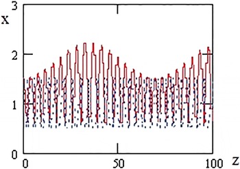
A similar model was shown to be relevant for the description of a sheet beam with non-uniform charge distribution, i.e. when the self-forces and hence the oscillations inside the beam are nonlinear. In the nonlinear case some additional assumptions should be made. For this aim, the modified one-dimensional invariant should be used (Barminova Reference Barminova2014), which allows us to study beams with both strong and weak nonlinearity. In figure 2 the case of a weak self-field nonlinearity, caused by the deviation of the charge distribution from uniformity, is illustrated. In figure 2 the dimensionless longitudinal coordinate $z$ is used instead of the time. This is valid if the drift velocity of the particles is a constant value. The oscillations of the envelope are demonstrated as having two characteristic frequencies. The envelope oscillations are obtained with the help of the kinetic distribution function of the same type as (2.9).

Figure 2.

Two frequency radius oscillations of a sheet beam in the case of a weak deviation of the field from linearity ( $x$ and $z$ are dimensionless transverse and longitudinal coordinates respectively).