




No CrossRef data available.
ASYMPTOTICS FOR GARCH SQUARED RESIDUAL CORRELATIONS
Published online by Cambridge University Press: 06 June 2003
Abstract
We develop an asymptotic theory for quadratic forms of the autocorrelations of squared residuals from a GARCH(p,q) model. Denoting by 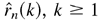 , k ≥ 1, these autocorrelations computed from a realization of length n, we show that the statistic
 is a matrix computed from the data, converges to the chi-square distribution with K degrees of freedom for any 1 ≤ i1 < ··· < iK. Our results are valid under weak assumptions on the innovations and model coefficients that admit that arbitrary low-order moments of the observations can be infinite. The matrix
 and its asymptotic limit D depend on the distribution of the innovations. A small simulation study illustrates the theory and shows, in particular, that using the matrix D computed under the assumption of normal innovations may lead to incorrect conclusions if the innovations have a different distribution.We thank the two referees for their comments and Professor Bruce E. Hansen, the co-editor in charge, for his sound advice on how to improve the paper. The work of István Berkes was supported by the Hungarian National Foundation for Scientific Research, grant T 29621. The work of Lajos Horváth and Piotr Kokoszka was supported by NATO grant PST.CLG.977607.
Information
- Type
- Research Article
- Information
- Copyright
- © 2003 Cambridge University Press
1. INTRODUCTION
The present paper extends earlier results presented in Horváth and Kokoszka (2001), where the asymptotic distribution of sums of squared residual autocorrelations in an ARCH(p) model was considered under the assumption that the realizations have finite fourth moment. In practical applications, however, the most frequently used model is GARCH(1,1); see, e.g., Chapter 15 of Hull (2000) for an introduction and McNeill and Frey (2000) for a recent application. We consider the more general GARCH(p,q) model. If the parameters of a GARCH(p,q) are estimated by the quasi–maximum likelihood method (for the general results, cf. Lee and Hansen, 1994; Lumsdaine, 1996; Berkes, Horváth, and Kokoszka, 2001), it is implicitly assumed that the innovations have at least four finite moments.
The statistical methodology investigated in this paper is proposed by Li and Mak (1994) and Ling and Li (1997), who aim at developing portmanteau tests based on autocorrelations of squared residuals in a large class of heteroskedastic time series models. Using Gaussian formalism, they derive the asymptotic distributions of analogues of the Box–Pierce statistic. These authors assume the conditional normality and finite fourth moments of the observations. As argued by Lee and Hansen (1994) (for an empirical study, see also Guillaume, Dacorogna, Dave, Müller, Olsen, and Pictet, 1997), these assumptions need not necessarily be satisfied by models and time series encountered in econometric applications, and so an analogous theory under more general assumptions should be developed. As in Lee and Hansen (1994) and Berkes et al. (2001) we do not assume that the innovations have a density, and we allow the observations to have arbitrarily heavy tails, so that even the expected value need not exist. We show that under these more general assumptions the estimated autocorrelations are asymptotically normal. We then apply our results to construct a GARCH(p,q) specification test. Goodness-of-fit tests based on model residuals have long been an established tool in diagnostic checking of time series models with additive noise; see, e.g., Chapter 8 of Box, Jenkins, and Reinsel, (1994) for an introduction and Hong (1996), de Jong (1996), and Bierens and Ploberger (1997) for some new approaches. In this paper we focus on a model with multiplicative noise.
Horváth, Kokoszka, and Teyssiére (2001) obtains the asymptotic distribution of the sequential empirical process of the squared residuals of ARCH(p) processes and shows that it does not converge to a standard Gaussian process, so, in contrast to the approach considered in the present paper, it is unlikely that asymptotically pivotal goodness-of-fit tests based on the empirical process can be developed. Berkes and Horváth (2002) extend the results of Horváth et al. (2001) to the setting considered in this paper whereas Horváth, Kokoszka, and Teyssiére (2002) study by means of simulations the corresponding bootstrap tests.
A GARCH(p,q) process is defined by the equations

and

where

are constants. We also assume that

Nelson (1990) shows that in the case of GARCH(1,1) sequence, (1.1) and (1.2) have a unique stationary solution if and only if E log(β1 + α1ε02) < 0. Bougerol and Picard (1992a, 1992b) find necessary and sufficient conditions for the existence of a unique stationary solution of (1.1) and (1.2) in the case of general GARCH(p,q). To state their condition we must introduce further notation. Let

(Clearly, without loss of generality we may and shall assume min(p,q) ≥ 2.) Define the (p + q − 1) × (p + q − 1) matrix An, written in block form, by

where Iq−1 and Ip−2 are the identity matrices of size q − 1 and p − 2, respectively. The norm of any d × d matrix is defined by

where ∥·∥ is the usual (Euclidean) norm in

. The top Lyapunov exponent γL associated with the sequence {An,−∞ < n < ∞} is

assuming that

(We note that ∥A0∥ ≥ 1; cf. Berkes et al., 2001.) Bougerol and Picard (1992a, 1992b) show that if (1.5) holds, then (1.1) and (1.2) have a unique stationary solution if and only if

Throughout this paper we will assume that conditions (1.1)–(1.6) hold. Clearly, they are a minimal set of conditions for the existence and stationarity of the GARCH(p,q) sequence.
Lumsdaine (1996) studies the quasi–maximum likelihood estimator of θ = (ω,α1, α2,…,αp,β1,β2,…,βq) from y1,y2,…,yn and proves its (weak) consistency and asymptotic normality for the GARCH(1,1) model. We wish to note that the consistency (and therefore the asymptotic normality also) is local; i.e., in the definition of the quasi–maximum likelihood estimator, the maximum of the likelihood function is computed in a small neighborhood of θ. Berkes et al. (2001) remove some unnecessary conditions assumed by Lumsdaine (1996) and extend the almost sure consistency and asymptotic normality to GARCH(p,q) sequences. The conditions in Berkes et al. (2001) are essentially optimal, so we follow their approach.
We continue with the formal definition of the quasi–maximum likelihood estimator for θ. First we define a sequence of functions by a recursion. Let

, then

and if q < p, the preceding equations are replaced with

If i > max(p,q), then

The logarithm of the quasi-likelihood function of the sample y1,y2,…,yn is given by

where

The quasi–maximum likelihood estimator is defined as

where U is given by

2. MAIN RESULTS
If the innovations ε1,…,εn were observable, an estimator for the autocovariance function of the squared innovations would be

(We assume in (2.5), which follows, that Eε02 = 1.) Because ε12,…,εn2 are not observable, we replace them with the squared residuals

and we shall use

Our first result compares

. First we list the conditions that are shown in Berkes et al. (2001) to be sufficient for the asymptotic normality of

:


and

If k gets large then

of (1.7) can be replaced with

Here the infinite series converges with probability one by Lemmas 4.1 and 4.4 and relation (5.4), which follow. Let

We show in Section 4 that ck is finite. We use uT to denote transpose of a vector or a matrix.
THEOREM 2.1. If (2.1)–(2.6) hold, then for any 0 ≤ k < ∞

According to Theorem 2.1 the first-order properties (i.e., the mean, law of large numbers) are the same for

as for rn(k). However, they differ in the second-order properties (i.e., variance, central limit theorem).
Theorem 2.1 implies the asymptotic normality of

for any 1 ≤ k < ∞. To get χ2-statistics we shall prove the joint asymptotic normality of

for any 1 ≤ i1 < i2 < ··· < iK. We start with the description of the asymptotic covariance matrix of

. Let

and

where

We note that the matrices in (2.10) and (2.11) have already appeared in the asymptotic covariance matrix of

(cf. Berkes et al., 2001) and they were proved to be nonsingular. Their appearance in our theorems is due to the presence of

in the definition of the squared residuals. For any 1 ≤ K < ∞ and 1 ≤ i1 < i2 < ··· < iK let D be the matrix with elements

THEOREM 2.2. If (2.1)–(2.6) hold, then

where N(0,D) stands for a multivariate normal random variable with mean 0 and covariance matrix D.
Remark 1.1. Berkes et al. (2001) prove that A0 = −B0, if Eε04 = 3 which is satisfied, e.g., if ε0 is standard normal. In this case D(k,k) = 4 + cikB0−1cikT and

.
Li and Mak (1994) and Ling and Li (1997) assume that conditionally on the past the y's have normal distribution. In our setting, this reduces to standard normal innovations εi. In this case, our results accord with those of these authors.
The covariance matrix in Theorem 2.2 has a very special structure. Let C be the K × (p + q + 1) matrix defined as

and let IK denote the K × K identity matrix. Using this notation we can write

where

THEOREM 2.3. If (2.1)–(2.6) hold and

then

Theorem 2.3 yields that D−1 exists. The existence of D−1 is used in Li (1992), Li and Mak (1994), and Ling and Li (1997) without proving it.
Combining Theorems 2.2 and 2.3 we get the convergence in distribution of quadratic forms of

.
THEOREM 2.4. If (2.1)–(2.6) hold, then

where χ2(K) denotes a chi-square random variable with K degrees of freedom.
The matrix D is unknown in Theorems 2.2 and 2.3, and so these results cannot be applied immediately. However, D can be easily estimated from the data. Let

We note that

if n is large enough. Hence

can be used to estimate A0. We use

to estimate B0, ck, and d02, respectively. Let

Replacing d0, C, and S with the corresponding estimators in (2.13) and (2.14) we get

, our estimator for D−1.
THEOREM 2.5. If (2.1)–(2.6) hold, then

where χ2(K) denotes a chi-square random variable with K degrees of freedom.
The proofs of Theorems 2.1–2.4 will be postponed until Section 5. Next we discuss a small simulation study to illustrate the applicability of our results.
3. A SIMULATION STUDY
The goal of the small simulation study that we performed in conjunction with the theoretical research presented in this paper was to develop some idea on how the goodness-of-fit procedures we propose might perform in finite samples. The results presented here are intended only to highlight some points of interest and are by no means intended as a guide for practitioners. If anything, we hope that our research and the simulation results presented in this section will encourage further investigation of these tests, and this should lead to a better fine-tuning of the finite sample procedures. It is also possible that a more extensive simulation study would modify our tentative conclusions.
In all our simulations we estimated the GARCH(1,1) model, which is most frequently used in practice. Under the null hypothesis the simulated series follow the GARCH(1,1) model, and under the alternative they do not follow GARCH(1,1). Ling and Li (1997) perform a similar simulation study assuming that the errors are normal. For this reason we focus here on nonnormal errors. We wanted to shed some light on the following questions.
(1) If the innovations are very different from normal, but the underlying model is correctly specified, is there a distinct possibility of arriving at incorrect conclusions if one uses the statistic proposed by Ling and Li (1997) (which was derived under the assumption of Gaussian errors and should be used only for such errors)?
(2) Ling and Li (1997) assume finite fourth moment of the observations, but our theoretical results are valid without this assumption. Do the tests have correct size in finite samples when the fourth moment is infinite?
Beyond these two questions, we would like to see how much is gained by applying the procedures proposed by Ling and Li (1997) and developed in this paper rather than using the “standard” statistic

and to have some idea about the power of the test against some typical alternatives.
With these questions in mind we considered the following test statistics:

where

is the estimator from Theorem 2.5. The analogue of the statistic Q(K) in situations in which we know that the errors are standard normal (or at least have the same first four moments as a standard normal random variable; cf. Remark 1.1) is

where

is the estimator of

obtained by replacing C and B0 with the estimates proposed in Section 2. We also take a look at the statistic

to see what conclusions a researcher not familiar with the theory developed in this paper and the work of Ling and Li (1997) might arrive at if he or she incorrectly used the “usual” statistic Q*(K). In our simulations, we treated Q*(K) as if it had the asymptotic chi-squared distribution with K degrees of freedom (in analogy to Q(K)). If we treated it, as is usual in case of ARIMA models, as if it had less than K degrees of freedom, its performance would be even worse.
We present here detailed results for two models:

The parameters of the model N1 are typical for daily stock returns, whereas model N2 has very heavy tails: P(|y| > u) ∼ cu−2, so that even the variance of the observations is infinite.
We considered sample of sizes 250 and 500. These are natural sample sizes if one wants to model daily returns on speculative assets because there are about 250 trading days per year. The empirical sizes are based on 1,000 replications, and so the standard error of the size estimates is about 0.005.
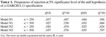
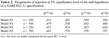
Comparing the entries in Tables 1 and 2, we see that using the “Gaussian” matrix

instead of the matrix

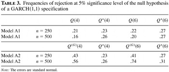
can lead to enormous size distortions if the errors are far from normal, double exponential in this case. In such cases using the statistic Q*(K) instead of the correct statistic Q(K) also causes a very large size distortion (see Table 1). The latter effect is not so noticeable if the innovations are normal, as can be gleaned from Table 3, which also shows that in such cases using the matrix

gives better results than using

. To estimate D one has to estimate d02 and A0, and this is not required when estimating D(G).
Frequencies of rejection at 5% significance level of the null hypothesis of a GARCH(1,1) specification

Frequencies of rejection at 5% significance level of the null hypothesis of a GARCH(1,1) specification

Frequencies of rejection at 5% significance level of the null hypothesis of a GARCH(1,1) specification

The empirical sizes of tests based on the statistic Q(K) (see Table 1), are smaller than the nominal size of .05, even though the sample size of n = 500 is quite large. The situation here appears to be quite similar to what has been observed for the statistic Q*(K) in the context of ARIMA models (see Box et al., 1994, Section 8.2.2, where a discussion and further references are provided). To address this problem Ljung and Box (1978) modify the statistic Q*(K) by using a more accurate approximation for the variance of the white noise autocorrelations. It might be interesting to see if such a finite sample correction is possible in the present setting. For samples of size n = 103 and the statistic Q(K) the empirical size is around .04, but in applications stationarity of such long samples may be questionable. Observe that for model N1 (see Tables 1 and 2) the empirical size appears to be closer to the nominal size for n = 250 than for n = 500. We repeated these simulations with different sets of random numbers and slightly different models and this anomaly appears to exist when β is close to 1 and α close to zero. It does not appear for other choices of parameters (e.g., model N2).
To investigate the power of the tests we focused on two alternatives

For sample sizes of 250 and 500 the power for the statistic Q(K) ranges from 0.1 to 0.3, which accords with the low empirical size reported previously.
In conclusion, our limited simulation study indicates that the goodness-of-fit tests based on the statistics studied in this paper may be quite useful when finite sample approximations to their distributions are better understood, but even in the present form they may serve as preliminary diagnostic tools. Our study clearly establishes that it is not acceptable to use tests derived under the assumption of the normality of errors if these are far from normal.
4. SOME TECHNICAL RESULTS
We start with a partial sum representation of

.
THEOREM 4.1. If (2.1)–(2.6) hold, then


and

Proof. Lee and Hansen (1994) and Lumsdaine (1996) obtain (4.1)–(4.3) for GARCH(1,1) under stronger conditions. Theorem 4.1 is proved by Berkes et al. (2001) under the present conditions for general GARCH(p,q) processes.
LEMMA 4.1. If (2.1)–(2.6) hold, then there is δ* > 0 such that

Proof. Lemma 2.3 of Berkes et al. (2001) yields (4.4).
For any γ > 0 let U(γ) = {u ∈ U : ∥θ − u∥ ≤ γ}. █
LEMMA 4.2. If (2.1)–(2.6) hold, then for any −∞ < ν < ∞ there is a 0 < γ < ∞ such that

Also, for any κ > 0

and

Proof. The result in (4.5) is a special case of Lemma 3.7 in Berkes and Horváth (2001).
Combining Lemmas 3.2, 3.3, and 5.2 in Berkes et al. (2001) and Lemma 4.1 we immediately obtain (4.6) and (4.7) (cf. also Berkes and Horváth, 2001, Lemma 3.4).
The next lemma wil be used to show that D−1 exists. Let 1 ≤ i1 < i2 < … iK and define

where

are constants.
LEMMA 4.3. If (2.1)–(2.6) and (2.15) hold, then Dμ* = EμTμ is nonsingular and positive definite.
Proof. Condition (2.6) and Lemma 4.2 imply that E∥μ∥2 < ∞ and therefore Dμ* exists. Thus it is enough to prove that Dμ* is nonsingular.
We assume that Dμ* is singular and show that this assumption leads to contradiction. If Dμ* is singular, then there are λ0 and (λ1,…,λK) ≠ 0 such that

Hence by (2.7) and Berkes et al. (2001) there are constants γ0,γ1,… satisfying |γi| = O(ρ*i) with some 0 < ρ* < 1 such that

By (1.1) and (1.2) we have that

Replacing w0(θ) in (4.8) with the expression in (4.9) we obtain that

It follows from the definition of the GARCH sequence that Z is measurable with respect to σ(ε−22,ε−32,…), the σ-algebra generated by ε−22,ε−32,…. Equation (4.10) yields that

Condition (2.15) implies that

and because σ−12 ≥ ω > 0, the right-hand side of (4.11) is finite almost surely. If i1 > 1 or i1 = 1 and λ1 = 0, then the right-hand side of (4.11) is measurable with respect to the σ(ε−22,ε−32,…). By (2.1) this contradicts (1.4).
Now we assume that i1 = 1 and λ1 ≠ 0. We can rewrite (4.11) as

The preceding equation is a quadratic function of ε−12. Because the coefficients are measurable with respect to σ(ε−22,ε−32,…), the solution, ε−12, must be measurable with respect to σ(ε−22,ε−32,…), contradicting (1.4) and (2.1). █
The last lemma will be used to estimate the difference between wk(u) and

. Let log+x = log x if x ≥ 1 and 0 otherwise. It is Lemma 2.2 of Berkes et al. (2001) and we state it here for easy reference. We denote log+x = log x if x ≥ 1 and 0 otherwise.
LEMMA 4.4. If {ξk,0 ≤ k < ∞} is a sequence of identically distributed random variables satisfying

then

converges with probability one for any |z| < 1.
5. PROOFS OF THEOREMS 2.1–2.4
Let

Elementary algebra gives

and similarly

where

LEMMA 5.1. If (2.1)–(2.6) hold, then there is γ > 0 such that

for all δ′ < δ, where δ is defined in (2.6).
Proof. By Lemma 3.1 in Berkes et al. (2001) there is a constant C1 such that

Hence,

where

. By Lemmas 4.1 and 4.4 ζ is finite with probability one.
Because c0(u) ≥ u1 > 0 and ci(u) ≥ 0 for all u ∈ U, we get

because of (5.5). Again using Lemmas 4.1 and 4.4 we conclude that

By (2.6) we have that

and therefore by (5.6) we have

Proceeding as in (5.6), by (5.5), (5.7), and (5.8) we have

Next we write

By (5.5) we conclude

Using the definitions of wi(u) and

with (5.4) and (5.5) we get for any u ∈ U

Hence (5.7) implies

By (5.7) and (5.8) we have

Let 0 < δ′ < δ and choose δ* so that δ′ < δ* < δ. Using (4.5) we see that there are γ > 0 and C2 such that

Because

are independent, by (5.12) and the Markov inequality we have

and therefore the Borel–Cantelli lemma implies

Thus we showed that

resulting in

Similar arguments yield

Lemma 5.1 now follows from (5.9)–(5.11), (5.13), and (5.14). █
For any 0 < L < ∞ let

LEMMA 5.2. If (2.1)–(2.6) hold, then for any 0 ≤ k < ∞ and 0 < L < ∞ we have

as n→∞.
Proof. Using Taylor expansion for wi−1(u) we get

where ξi satisfies ∥ξi − θ∥ ≤ ∥u − θ∥. The Hölder inequality, (2.6), and (4.6) yield E∥(εi−k2 − 1)wi′(θ)/wi(θ)∥ < ∞. So by (2.5) and the independence of εi2 and εi−k2wi′(u)/wi(u) we have

For any 1 ≤ k < ∞, {εi2(εi−k2 − 1)wi′(θ)/wi(θ), −∞ < i < ∞} is a stationary and ergodic sequence (cf. Stout, 1974, Theorem 3.5.8) with finite mean, so by the ergodic theorem we conclude

Hence

Next we write

By the Hölder inequality for all large enough n we have

where in the last step we used the Cauchy inequality, (2.6), and Lemma 4.2. Again using the ergodic theorem we get

as n→∞. Similarly to (5.18) one can verify that

as n→∞. Putting together (5.16)–(5.19) we obtain that

as n→∞.
Repeating the arguments leading to (5.16) we conclude

where ξi−k satisfies ∥ξi−k − θ∥ ≤ ∥u − θ∥. Because εi2 and {εi−k2,wi−k′(θ)/ wi−k(θ)} are independent, by (2.5) and Lemma 4.2 we have

So the ergodic theorem yields

as n→∞ for any 0 < L < ∞. Similarly to (5.18) and (5.19) we have

Thus we have established that

Using the mean value theorem we conclude

so following the proof of (5.18), using Lemma 4.2 and the ergodic theorem we have

Lemma 5.2 now follows from (5.1) and (5.20)–(5.22). █
Proof of Theorem 2.1. Putting together Lemmas 5.1 and 5.2 we get that for any 0 ≤ k < ∞ and L < ∞

as n→∞. We note that the random vectors (1 − εi2)wi′(θ)/wi(θ), −∞ < i < ∞ are uncorrelated and have bounded second moments, so by the Chebyshev inequality we have

Thus by (4.3) we get

and therefore Theorem 2.1 follows from (5.23). █
Proof of Theorem 2.2. By Theorems 2.1 and 4.1 it is enough to prove that

We note that η1, η2,… are uncorrelated, stationary random vectors. It is easy to see that Eηj = 0 and because

(cf. Berkes et al., 2001, the proof of Remark 4.5) we get EηjTηj = D.
Next we observe that η1, η2,… is a stationary, ergodic process. It is also a martingale difference sequence with respect to the σ-algebras generated by {εj,−∞ < j < i} with finite second moments. Using the Cramér–Wold theorem (cf. Billingsley, 1968, p. 49) and Theorem 23.1 of Billingsley (1968, p. 206) we obtain (5.25). █
Proof of Theorem 2.3. We note that

where zj = cij(B0−1)T/2. Thus (2.6) follows from Lemma 4.3. █
Proof of Theorem 2.4. It is an immediate consequence of Theorem 2.2 and (2.16). █
Let

LEMMA 5.3. If (2.1)–(2.6) hold, then there is γ > 0 such that A0(u),B0(u), and ck(u) exist for all u ∈ U(γ),


and

as n→∞.
Proof. It is easy to see that

Using the Hölder inequality, (2.6), (4.5), and (4.6) we conclude

for all u ∈ U(γ) assuming that γ > 0 is small enough. The existence of B0(u) is proved in Lemma 5.6 of Berkes et al. (2001). By the Cauchy inequality, (2.6), and (4.6) we have

establishing the existence of ck(u) for all u ∈ U.
Observing that

(5.27) is proved in Berkes et al. (2001). The proofs of (5.26) and (5.28) are similar so we provide an outline for (5.28) only. Following the proof of Lemma 5.1 one can verify that with a small enough γ > 0

Introducing

we write

Applying (5.5) there is a random variable ζ* such that

by (4.6) and Lemmas 4.1 and 4.4. Using the mean value theorem we get with a small enough γ that

By (2.6) and Lemma 4.2 we obtain

and therefore by the ergodic theorem we have

So (5.24) yields

with some γ > 0. The ergodic theorem implies that

and

Putting together (5.30) and (5.31) we conclude by standard arguments

completing the proof of (5.28).
Because by the independence of ε0 and w0′(θ)/w0(θ) we have that c0 = 0, (5.29) follows from Theorem 2.1 and the strong law of large numbers. █
Proof of Theorem 2.5. Lemma 5.3 and (5.24) imply

and therefore the result follows from the central limit theorem in Theorem 2.4. █
References
REFERENCES
Berkes, I. &
L. Horváth
(2001)
The Efficiency of the Estimators of the Parameters in GARCH
Processes.
Preprint.
Berkes, I. &
L. Horváth
(2002)
Limit Results for the Empirical Process of Squared Residuals in GARCH
Models.
Preprint.
Berkes, I.,
L. Horváth, &
P. Kokoszka
(2001)
GARCH processes: Structure and estimation.
Bernoulli.
Forthcoming.
Bierens, H.J. &
W. Ploberger
(1997)
Asymptotic theory of integrated conditional moment tests.
Econometrica
65,
1129–1151.CrossRefGoogle Scholar
Billingsley, P.
(1968)
Convergence of Probability Measures.
New York:
Wiley.
Bougerol, P. &
N. Picard
(1992a)
Strict stationarity of generalized autoregressive processes.
Annals of Probability
20,
1714–1730.Google Scholar
Bougerol, P. &
N. Picard
(1992b)
Stationarity of GARCH processes and of some nonnegative time series.
Journal of Econometrics
52,
115–127.Google Scholar
Box, G.E.P,
G.M. Jenkins, &
G.C. Reinsel
(1994)
Time Series Analysis: Forecasting and Control,
3rd ed.
Englewood Cliffs, New Jersey:
Prentice Hall.
de Jong, R.M.
(1996)
The Bierens test under data dependence.
Journal of Econometrics
72,
1–32.CrossRefGoogle Scholar
Guillaume, D.M.,
M.M. Dacorogna,
R.D. Dave,
U.A. Müller,
R.B. Olsen, &
O.V. Pictet
(1997)
From the bird's eye to the microscope: A survey of new
stylized facts of the intra-daily foreign exchange markets.
Finance and Stochastics
1,
95–129.CrossRefGoogle Scholar
Hong, Y.
(1996)
Consistent testing for serial correlation of unknown form.
Econometrica
64,
837–864.CrossRefGoogle Scholar
Horváth, L. &
P. Kokoszka
(2001)
Large sample distribution of weighted sums of ARCH(p)
square residual correlations.
Econometric Theory
17,
283–295.CrossRefGoogle Scholar
Horváth, L.,
P. Kokoszka, &
G. Teyssiére
(2001)
Empirical process of the squared residuals of an ARCH sequence.
Annals of Statistics
29,
445–469.Google Scholar
Horváth, L.,
P. Kokoszka, &
G. Teyssiére
(2002)
Bootstrap Specification Tests for ARCH Based on the Empirical Process
of the Squared Residuals.
Preprint.
Hull, J.C.
(2000)
Options, Futures, and Other Derivatives.
Upper Saddle River, New Jersey:
Prentice Hall.
Lee, S.-W. &
B.E. Hansen
(1994)
Asymptotic theory for the GARCH(1,1) quasi-maximum likelihood
estimator.
Econometric Theory
10,
29–52.CrossRefGoogle Scholar
Li, W.K.
(1992)
On the asymptotic distribution of residual autocorrelations in
nonlinear time series modelling.
Biometrika
79,
435–437.CrossRefGoogle Scholar
Li, W.K. &
T.K. Mak
(1994)
On the squared residual autocorrelations in non-linear time series
with conditional heteroskedasticity.
Journal of Time Series Analysis
15,
627–636.CrossRefGoogle Scholar
Ling, S. &
W.K. Li
(1997)
On fractionally integrated autoregressive moving–average time
series models with conditional heteroscedasticity.
Journal of the American Statistical Association
92,
1184–1194.CrossRefGoogle Scholar
Ljung, G. &
G. Box
(1978)
On a measure of lack of fit in time series models.
Biometrika
66,
67–72.CrossRefGoogle Scholar
Lumsdaine, R.L.
(1996)
Consistency and asymptotic normality of the quasi–maximum
likelihood estimator in IGARCH (1,1) and covariance stationary GARCH
(1,1) models.
Econometrica
6,
575–596.CrossRefGoogle Scholar
McNeill, A.J. &
R. Frey
(2000)
Estimation of tail-related risk measures for heteroskedastic
financial time series: An extreme value approach.
Journal of Empirical Finance
7,
271–300.CrossRefGoogle Scholar
Nelson, D.B.
(1990)
Stationarity and persistence in GARCH(1, 1) model.
Econometric Theory
6,
318–334.CrossRefGoogle Scholar
Stout, W.F.
(1974)
Almost Sure Convergence.
New York:
Academic Press.
Frequencies of rejection at 5% significance level of the null hypothesis of a GARCH(1,1) specification
Frequencies of rejection at 5% significance level of the null hypothesis of a GARCH(1,1) specification
Frequencies of rejection at 5% significance level of the null hypothesis of a GARCH(1,1) specification
 You have
Access
- 33
- Cited by