


1. INTRODUCTION
Let X denote the steady-state number of customers in the system for the first come–first served M/G/1 queue. Imagine that, for a specified n, the nth oldest customer in the system (if there are at least n in the system) pays us 1 per unit time. Then, with λ being the Poisson arrival rate and with S being a generic service time random variable, we obtain, upon applying the cost identity,

along with the PASTA principle, that when n = 1

and for n > 1,

where Rj is the remaining time in service of the person being served when a customer arrives to find j others in the system.
Thus, with

we see that

Thus,

giving

Remarks:
1. Equations (1) and (2) are neatly summarized in terms of the failure rate function r(n) = P(X = n|X ≥ n) = 1 − P(X ≥ n + 1|X ≥ n). With E [R0] = E [S],

with

2. BOUNDS
If we let

then

The preceding bounds can be particularly useful in cases where we only have partial information about G.
Example 1: If S has the new worse than used in expectation property (NWUE) that

then m1 = E [S], showing that

In other words, X is stochastically larger (in fact, hazard rate larger) than when the service distribution is exponential with mean E [S]. Similarly, if S has the new better than used in expectation property that E [S − t|S ≥ t] ≤ E [S], then m2 = E [S], showing in this case that

Example 2: Suppose that all that is known about the service distribution is its mean and that it is a mixture of exponential random variables with respective means θ1 > θ2 > ··· > θm. Because S is NWUE, and the conditional distribution of S given that it exceeds t is a mixture of the exponentials whose weight on θ1 goes to 1 as t → ∞, we have that m1 = E [S] and m2 = θ1. Therefore,

Example 3: Suppose that S is a convolution of exponential random variables with respective means θ1 > θ2 > ··· > θm. Because S is an increasing failure rate random variable whose limiting failure rate is 1/θ1, it follows that m1 = θ1. Thus, provided θ1 and E [S] are known, we have

To obtain stronger bounds than those given in the preceding, let S,W1,W2,… be independent, with S having the service time distribution and the Wi being exponential random variables with rate λ. Let

and let

Then, with Fj denoting the distribution function of Yj (viz. gamma with parameters j and λ), a simple computation yields

with the formula for α1 simplifying to
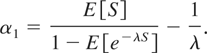
Now consider a customer, call it *, that finds j, j > 0, in the system upon arrival. Letting M denote the number of customers (including *) that have so far arrived while the current service has been in progress, then the remaining service time is distributed as the conditional distribution of S − YM conditional on the event that S > YM. Conditioning on M shows that E [Rj] is a weighted average of the values α1,…, αj, yielding the bounds

Now suppose that S has the decreasing mean residual life time (DMRL) property that E [S − t|S > t] decreases in t. Because the exponential distribution has a decreasing reversed hazard rate, it follows that the conditional distribution of Yj, given that Yj < S, is stochastically increasing in j (see [3]). Consequentially, it follows from the DMRL property of S that αj is decreasing in j, showing that

which implies

Similarly, if S has the increasing mean residual life time property that E [S − t|S > t] increases in t, then



