2. First alarm triggering

Consider the first alarm if it actually occurs. The process (1.1) is then stopped at the time

(2.1) \begin{equation}\tau_1 = \inf\{t>0\,:\, A_t=1 \mbox{ or } I_t=0\}.\end{equation}

If the population ends by an alarm, the stopping state has the form $(A_{\tau_1}=1, I_{\tau_1}=i)$ , $i\geq 1$ . Conversely, if the population dies out before any alarm, the stopping state is $(A_{\tau_1}=0, I_{\tau_1}=0)$ . Note that $A_{\tau_1}=\min(I_{\tau_1},1)$ , so that only $I_{\tau_1}$ needed to be retained.

Our goal in this section is to determine the PGF of the population state $(I_{\tau_1}, R_{\tau_1})$ . For that, we will use simple martingale arguments and the optional stopping theorem. We start by looking for a martingale of the form

(2.2) \begin{equation}M_t=f(I_t,R_t,A_t), \qquad t\geq 0,\end{equation}

with respect to $\mathcal{F}_t=\sigma\{(I_u,R_u,A_u),\, 0\leq u\leq t\}$ , where f(i, r, a) is a real function to choose.

Lemma 2.1. $\{M_t,\, t\geq 0\}$ is a martingale if the values f(i, r, a) satisfy the conditions

(2.3) \begin{equation}f(i+1,r,a) \lambda + f(i-1,r+1,a) \mu + f(i,r,a+1) \alpha = f(i,r,a) (\lambda+\mu+\alpha), \quad i\geq 1.\end{equation}

Proof. Let $m_t=\mathbb{E}(M_t \mid \mathcal{F}_{t_0})$ , $t\geq t_0$ . From (1.1), we have

\begin{align*}m_{t+{\rm d} t} &=\mathbb{E}\bigl\{\,f(I_t+1,R_t,A_t) \lambda I_t {\rm d} t + f(I_t-1,R_t+1,A_t) \mu I_t {\rm d} t + f(I_t,R_t,A_t+1) \alpha I_t {\rm d} t \\[2pt] &\qquad +\, f(I_t,R_t,A_t) [1- (\lambda+\mu+\alpha) I_t {\rm d} t]\bigr\} + o({\rm d} t),\end{align*}

so that the derivative of m(t) satisfies the equation

(2.4) \begin{align}m_t^\prime &= \mathbb{E}\bigl\{I_t\bigl[f(I_t+1,R_t,A_t) \lambda + f(I_t-1,R_t+1,A_t) \mu + f(I_t,R_t,A_t+1) \alpha\nonumber \\[2pt] &\qquad - f(I_t,R_t,A_t) (\lambda+\mu+\alpha) \bigr]\bigr\}.\end{align}

The martingale condition requires that $m_t^\prime=0$ for all $t\geq t_0$ . From (2.4), this condition is obviously satisfied if $I_t=0$ . On the other hand, when $I_t=i\geq 1$ , the condition gives us the announced relations (2.3).

Let us now try as a particular case the function f defined by

(2.5) \begin{equation}f(i,r,a)=y^i z^r v^a,\end{equation}

where y, z are any reals in (0, 1] and $v\equiv v(y,z)$ is a real that will be taken accordingly.

Lemma 2.2. The function (2.5) satisfies the martingale conditions (2.3) if

(2.6) \begin{equation}v(y,z) = \frac{-\lambda y^2 +(\lambda+\mu+\alpha)y -\mu z}{\alpha y}.\end{equation}

The associated martingale (2.2) is then

(2.7) \begin{equation}M_t = y^{I_t} z^{R_t} [v(y,z)]^{A_t}, \qquad t\geq 0.\end{equation}

Proof. Substituting (2.5) in (2.3) gives

\begin{equation*}\lambda y^{i+1} z^r v^a + \mu y^{i-1} z^{r+1} v^a + \alpha y^{i} z^r v^{a+1} = (\lambda+\mu+\alpha) y^{i} z^r v^a, \qquad i\geq 1,\end{equation*}

which reduces to

\begin{equation*}\lambda y^2 + \mu z + \alpha y v = (\lambda+\mu+\alpha) y.\end{equation*}

For y, z fixed in (0, 1], this equality gives the expression (2.6) for $v=v(y,z)$ . The martingale (2.7) follows directly.

We are ready to derive the state distribution at the stopping time (2.1). Clearly, we can write

(2.8) \begin{align}\mathbb{E}\!\left(y^{I_{\tau_1}}z^{R_{\tau_1}}\right) &= \mathbb{E}\big(y^{I_{\tau_1}}z^{R_{\tau_1}}\textbf{1}_{(I_{\tau_1}=0)}\big) + \mathbb{E}\big(y^{I_{\tau_1}}z^{R_{\tau_1}}\textbf{1}_{(I_{\tau_1}>0)}\big)\nonumber \\[2pt] &= p_1(z) + \mathbb{E}\big(y^{I_{\tau_1}}z^{R_{\tau_1}}\textbf{1}_{(I_{\tau_1}>0)}\big),\end{align}

after setting

(2.9) \begin{equation}p_1(z)\equiv \mathbb{E}\big(z^{R_{\tau_1}}\textbf{1}_{(I_{\tau_1}=0)}\big).\end{equation}

The expectation (2.9) plays a key role in the following and will be determined in Proposition 2.4 below. Note that for $z=1$ , $p_1(1)=\mathbb{P}(I_{\tau_1}=0)$ , which represents the probability of extinction of the population before any alarm. The formula (2.8) can now be completed as follows.

Proposition 2.1. The PGF of $(I_{\tau_1}, R_{\tau_1})$ is given by

(2.10) \begin{equation}\mathbb{E}\!\left(y^{I_{\tau_1}}z^{R_{\tau_1}}\right) = p_1(z) - \frac{\alpha y [y-p_1(z)]}{\lambda y^2 - (\lambda+\mu+\alpha) y +\mu z}.\end{equation}

Proof. Let us stop the martingale (2.7) at the time $\tau_1$ . By the optional stopping theorem, we know that $\mathbb{E}(M_{\tau_1}\!) = M_0$ . Of course, $M_0=y$ since $(I_0,R_0, A_0)=(1,0,0)$ . Therefore,

(2.11) \begin{equation}\mathbb{E}(M_{\tau_1}\!) = \mathbb{E}\big(y^{I_{\tau_1}}z^{R_{\tau_1}} [v(y,z)]^{A_{\tau_1}}\big) = y.\end{equation}

Moreover, $\mathbb{E}(M_{\tau_1}\!)$ can be expressed as

(2.12) \begin{align}\mathbb{E}(M_{\tau_1}\!) &= \mathbb{E}\big[y^{I_{\tau_1}}z^{R_{\tau_1}}(v(y,z))^{A_{\tau_1}} \textbf{1}_{(I_{\tau_1}=0)}\big] + \mathbb{E}\big[y^{I_{\tau_1}}z^{R_{\tau_1}}(v(y,z))^{A_{\tau_1}} \textbf{1}_{(I_{\tau_1}>0)}\big]\nonumber \\[3pt] &= \mathbb{E}\big(z^{R_{\tau_1}}\textbf{1}_{(I_{\tau_1}=0)}\big) + v(y,z) \mathbb{E}\big(y^{I_{\tau_1}}z^{R_{\tau_1}}\textbf{1}_{(I_{\tau_1}>0)}\big) \nonumber\\[3pt] &= \mathbb{E}\big(z^{R_{\tau_1}}\textbf{1}_{(I_{\tau_1}=0)}\big) + v(y,z) \big[\mathbb{E}\big(y^{I_{\tau_1}}z^{R_{\tau_1}}\big) - \mathbb{E}\big(y^{I_{\tau_1}}z^{R_{\tau_1}}\textbf{1}_{(I_{\tau_1}=0)}\big)\big]\nonumber\\[3pt] &= p_1(z) + v(y,z) \big[\mathbb{E}\big(y^{I_{\tau_1}}z^{R_{\tau_1}}\big) - p_1(z)\big],\end{align}

using the notation (2.9). From (2.11) and (2.12), we obtain

\begin{equation*}y-p_1(z) = v(y,z) \big[\mathbb{E}\big(y^{I_{\tau_1}}z^{R_{\tau_1}}\big) - p_1(z)\big],\end{equation*}

and hence the desired result (2.10) after inserting (2.6).

It remains to determine $p_1(z)$ as announced. Since the rates $\mu, \alpha$ are positive, we notice from (2.9) that

(2.13) \begin{equation}0 < p_1(z) < 1, \qquad z\in (0,1].\end{equation}

Proposition 2.2. The expectation $p_1(z)$ is the root in (0, 1) of the quadratic equation

(2.14) \begin{equation}\lambda y^2 -(\lambda+\mu+\alpha) y + \mu z = 0.\end{equation}

Proof. Consider the quadratic equation (2.14). For $z \in (0,1]$ , we see that its two roots, denoted $y_1 (z)$ and $y_2 (z)$ , are such that $0 <y_1 (z) <1 <y_2 (z)$ . Thus, if $p_1 (z)$ is one of these roots, it is necessarily the smallest, $y_1 (z)$ .

Proceeding by contradiction, suppose that $p_1(z)$ is not a root of (2.14), i.e.

\begin{equation*}\lambda \left[p_1(z)\right]^2 - (\lambda+\mu+\alpha) p_1(z) + \mu z \neq 0.\end{equation*}

As a consequence, we may choose $y=p_1(z)$ in the formula (2.10), which gives the identity

(2.15) \begin{equation}\mathbb{E}\Big(\!\left[p_1(z)\right]^{I_{\tau_1}}z^{R_{\tau_1}}\!\Big) = p_1(z).\end{equation}

Let us expand the left-hand side of (2.15) depending on whether the value of $I_{\tau_1}$ is null or not. Using (2.9), the formula (2.15) becomes

(2.16) \begin{equation}p_1(z) + \mathbb{E}\Big(\!\left[p_1(z)\right]^{I_{\tau_1}} z^{R_{\tau_1}} \textbf{1}_{(I_{\tau_1} >0)}\Big) = p_1(z).\end{equation}

The solution $p_1(z)=0$ is excluded by (2.13). Since $p_1(z)>0$ , the identity (2.16) implies that $\mathbb{P}(I_{\tau_1}>0)=0$ or, equivalently, $p_1(1)=1$ . This is in contradiction with (2.13).

The formula (2.10) provides us with the PGF of $I_{\tau_1}$ . We are going to derive an explicit formula for the distribution itself of $I_{\tau_1}$ . Remember that $\mathbb{P}(I_{\tau_1}\geq 1)=1-p_1(1)$ .

Corollary 2.1. We have

(2.17) \begin{equation}\mathbb{P}\!\left(I_{\tau_1}=i \mid I_{\tau_1}\geq 1 \!\right) = (\!1-\pi_1\!)\pi_1^{i-1}, \qquad i\geq 1,\end{equation}

where $\pi_1 \in (0,1)$ is given by

(2.18) \begin{equation}\pi_1 = \lambda p_1(1)/\mu\qquad (\!=1/y_2(1)).\end{equation}

Proof. From (2.10) with $z=1$ , we get

(2.19) \begin{equation}\mathbb{E}\!\left(y^{I_{\tau_1}}\right) = p_1(1) - \frac{\alpha y [y-p_1(1)]}{\lambda y^2 - (\lambda+\mu+\alpha) y +\mu}.\end{equation}

On the right-hand side of (2.19), the quadratic form has two roots $y_1(1), y_2(1)$ such that $y_1(1)y_2(1)=\mu/\lambda$ and $y_1(1)=p_1(1)$ , hence $y_2(1)=\mu/\lambda p_1(1)$ ( $>1$ ). We thus see that $y_2(1)=1/\pi_1$ in the notation (2.18). Then, the formula (2.19) becomes

(2.20) \begin{align}\mathbb{E}\!\left(y^{I_{\tau_1}}\right) &= p_1(1) - \frac{\alpha y}{\lambda [y-\mu/\lambda p_1(1)]}\nonumber\\[3pt] &= p_1(1) + \frac{\alpha \pi_1 y}{\lambda (1 -\pi_1 y)}.\end{align}

Moreover, since $p_1(1)$ is a root of (2.14) with $z=1$ , we have the equality

\begin{equation*}-\lambda p_1(1)[1-p_1(1)]-\alpha p_1(1)+\mu[1-p_1(1)] =0,\end{equation*}

which yields, after division by $\mu[1-p_1(1)]$ and using (2.18),

(2.21) \begin{equation}\frac{\alpha\pi_1}{\lambda[1-p_1(1)]}=1-\pi_1.\end{equation}

Inserting (2.21), we can rewrite (2.20) as

\begin{align*}\mathbb{E}\!\left(y^{I_{\tau_1}}\right) &= p_1(1) + \frac{\alpha \pi_1 y}{\lambda (1 -\pi_1 y)}\frac{1-p_1(1)}{1-p_1(1)}\nonumber\\[3pt] &= p_1(1) + \frac{(1-\pi_1) y}{1 -\pi_1 y} [1-p_1(1)],\end{align*}

whose power series expansion in y is

\begin{equation*}\mathbb{E}\!\left(y^{I_{\tau_1}}\right) = p_1(1) +[1-p_1(1)] \sum_{i=1}^{\infty}(1-\pi_1) \pi_1^{i-1} y^{i}.\end{equation*}

The desired result (2.17) then follows.

By (2.17), we thus have the representation $(I_{\tau_1}\mid I_{\tau_1}\geq 1) \eqdist 1+G_1$ , where $G_1$ is a geometric random variable of parameter $1-\pi_1$ . In other words, given that an alarm is triggered at $\tau_1$ , the population size $I_{\tau_1}$ has a shifted geometric distribution. A similar result was obtained in [Reference Trapman and Bootsma17] in a close setting.

In particular, we obtain from (2.17) that

(2.22) \begin{equation}\mathbb{E}(I_{\tau_1}) = \frac{1-p_1(1)}{1-\pi_1} = \frac{1-p_1(1)}{1-\lambda p_1(1)/\mu}.\end{equation}

Let us look at the influence of the detection rate $\alpha$ . From (2.14), we see that $p_1(1)$ , the probability of extinction of the population at time $\tau_1$ , is a decreasing function of $\alpha$ , as waited intuitively. From (2.22), we deduce that $\mathbb{E}(I_{\tau_1})$ , the expected population size at $\tau_1$ , increases with $\alpha$ when $\lambda<\mu$ (i.e. if the population decreases on average).

From (2.10), we can also derive an explicit formula for the distribution of $R_{\tau_1}$ . For convenience, we set $\Big(\begin{array}{c}{0}\\{1}\end{array}\Big)\frac{1}{0}=1$ .

Corollary 2.2. We have

(2.23) \begin{align}\mathbb{P}(R_{\tau_1} = 0) &= \frac{\alpha}{\mu+\alpha}, \nonumber\\[3pt] \mathbb{P}(R_{\tau_1} = r) &= \frac{\alpha}{\mu+\alpha} \bigg(\frac{\mu}{\mu+\alpha}\bigg)^r + \frac{\mu}{\mu+\alpha}\, {\left(\begin{array}{c}{2r-2}\\[3pt] {r}\end{array}\right)} \frac{1}{r-1} \frac{\lambda^{r-1} \mu^{r}}{(\lambda+\mu+\alpha)^{2r-1}} \nonumber \\[3pt] & \quad - \sum_{k=1}^{r-1} \frac{\alpha}{\mu+\alpha} \bigg(\frac{\mu}{\mu+\alpha}\bigg)^{r-k} {\left(\begin{array}{c}{2k-2}\\{k}\end{array}\right)} \frac{1}{k-1} \frac{\lambda^{k-1} \mu^k}{(\lambda+\mu+\alpha)^{2k-1}}, \quad\ r\geq 1.\end{align}

Proof. From (2.10) with $y=1$ , we get

(2.24) \begin{align}\mathbb{E}\!\left(z^{R_{\tau_1}}\right) &= p_1(z) + \frac{\alpha [1-p_1(z)]}{ (\mu+\alpha) -\mu z}\nonumber\\[3pt] &= p_1(z) + [1-p_1(z)] \sum_{i=0}^{\infty}\frac{\alpha}{\mu+\alpha} \bigg(\frac{\mu}{\mu+\alpha}\bigg)^i z^i \nonumber\\[3pt] &= \sum_{i=0}^{\infty}\frac{\alpha}{\mu+\alpha} \bigg(\frac{\mu}{\mu+\alpha}\bigg)^i z^i + p_1(z) \frac{\mu}{\mu+\alpha} - p_1(z) \sum_{i=1}^{\infty}\frac{\alpha}{\mu+\alpha} \bigg(\frac{\mu}{\mu+\alpha}\bigg)^i z^i.\end{align}

Let us expand $p_1(z)$ as a power series in z. We recall that

\begin{equation*}(1+z)^{1/2} = \sum_{k=0}^{\infty}{\left(\begin{array}{c}{1/2}\\{k}\end{array}\right)} z^k = 1+ \sum_{k=1}^{\infty}{\left(\begin{array}{c}{2k-3}\\{k-1}\end{array}\right)} \frac{(\!-1)^{k-1}}{k2^{2k-2}} z^k,\end{equation*}

for any real z. From Proposition 2.2, we then obtain that

(2.25) \begin{align}p_1(z) &= \frac{\lambda+\mu+\alpha - [(\lambda+\mu+\alpha)^2-4\lambda \mu z]^{1/2}}{2\lambda}\nonumber\\[2pt] &= \frac{\lambda+\mu+\alpha}{2\lambda} \bigg\{1 - \bigg[1 - \frac{4\lambda \mu}{(\lambda+\mu+\alpha)^2} z\bigg]^{1/2}\bigg\}\nonumber\\[3pt] &= \frac{\lambda+\mu+\alpha}{2\lambda} \sum_{k=1}^{\infty}{\left(\begin{array}{c}{2k-3}\\{k-1}\end{array}\right)} \frac{1}{k2^{2k-2}} \frac{(4\lambda \mu)^k}{(\lambda+\mu+\alpha)^{2k}} z^k \nonumber\\[2pt] &= \sum_{k=1}^{\infty}{\left(\begin{array}{c}{2k-2 }\\{k}\end{array}\right)} \frac{1}{k-1} \frac{\lambda^{k-1} \mu^k}{(\lambda+\mu+\alpha)^{2k-1}} z^k.\end{align}

Inserting (2.25) in (2.24), we get a power series for the PGF of $R_{\tau_1}$ , which leads to the desired formula (2.23).

3. Multiple births and initial size

So far, the birth process can only generate one new individual, and the population has only one initial individual. These assumptions can, however, be relaxed.

3.1. Several possible offspring

For a branching with multiple births, the first transition probability in (1.1) is replaced by the probabilities of $k\, (\geq 1)$ possible births defined as

(3.1) \begin{equation}\mathbb{P}[(I_{t+{\rm d} t},R_{t+{\rm d} t},A_{t+{\rm d} t})= (i+k,r,a) \mid (I_t,R_t,A_t)=(i,r,a)]= \lambda_k i {\rm d} t + o({\rm d} t),\end{equation}

where $\lambda_k \geq 0$ with $\lambda \equiv \sum_{k=1}^{\infty}\lambda_k>0$ . The same martingale method is also applicable to this extended model.

Proposition 3.1. The PGF of $(I_{\tau_1}, R_{\tau_1})$ is given by

(3.2) \begin{equation}\mathbb{E}\!\left(y^{I_{\tau_1}}z^{R_{\tau_1}}\right) = p_{1}(z) - \frac{\alpha y [y-p_{1}(z)]}{\sum_{k=1}^{\infty}\lambda_k y^{k+1} - (\lambda+\mu+\alpha) y +\mu z},\end{equation}

in which $p_{1}(z)$ is the root in (0, 1) of the polynomial equation

(3.3) \begin{equation}\sum_{k=1}^{\infty}\lambda_k y^{k+1} - (\lambda+\mu+\alpha) y + \mu z = 0.\end{equation}

Proof. Under (3.1), the conditions (2.3) on f for having a martingale (2.2) become

\begin{equation*}\sum_{k=1}^{\infty}\lambda_k f(i+k,r,a) \lambda + f(i-1,r+1,a) \mu + f(i,r,a+1) \alpha = f(i,r,a) (\lambda+\mu+\alpha), \quad i\geq 1.\end{equation*}

For f given by (2.5), these conditions are satisfied if

\begin{equation*}v(y,z) = \frac{-\sum_{k=1}^{\infty}\lambda_k y^{k+1} +(\lambda+\mu+\alpha)y -\mu z}{\alpha y}.\end{equation*}

By arguing as for Propositions 2.1 and 2.2, we then obtain the announced results (3.2) and (3.3). Note that the equation (3.3) has a unique root in (0, 1) since the polynomial on the left is a convex function that is positive in $y=0$ and negative in $y=1$ .

For instance, if $\lambda_k$ is geometrically decreasing, i.e. $\lambda_k = ab^{k-1}$ , $k\geq 1$ ( $a>0,\ 0<b<1$ ), the formula (3.3) states that $p_{1}(z)$ is the root in (0, 1) of the quadratic equation

\begin{equation*}[a+b(1-b)(\mu+\alpha)]y^2-[a+(1-b)(\mu+\alpha+b\mu z)]y+(1-b)\mu z=0.\end{equation*}

3.2. Several initial individuals

Let us go back to the branching model (1.1), but now suppose that $I_0=m \, (\geq 1)$ . We can easily adapt the previous method to this situation. Denote by $p_1(z;\, m)$ the expectation (2.9), with $p_1(z; 1)\equiv p_1(z)$ .

Proposition 3.2. The PGF of $(I_{\tau_1}, R_{\tau_1})$ is given by

(3.4) \begin{equation}\mathbb{E}\!\left(y^{I_{\tau_1}}z^{R_{\tau_1}}\right) = (p_1(z))^m - \frac{\alpha y [y^m-(p_1(z))^m]}{\lambda y^2 - (\lambda+\mu+\alpha) y +\mu z}.\end{equation}

In particular, conditionally that the alarm is triggered first, $I_{\tau_1}$ is distributed as a mixture of m independent shifted geometric random variables, namely

(3.5) \begin{equation}\left(I_{\tau_1}\mid I_{\tau_1}\geq 1\right) \eqdist j+G_j \textit{\ with probability } c_j,\qquad j=1, \ldots, m,\end{equation}

where the $G_j$ are independent and identically distributed (i.i.d.) geometric random variables of parameter $1-\pi_1$ , and the $c_j$ are given by $c_j=(p_1(1))^{m-j}/\sum_{i=0}^{m-1}(p_1(1))^{i}$ .

Proof. Obviously, Lemmas 2.1 and 2.2 still hold. Instead of (2.11), we now have $\mathbb{E}(M_{\tau_1}\!) = y^m$ so that (2.10) in Proposition 2.1 is replaced by

\begin{equation*}\mathbb{E}\!\left(y^{I_{\tau_1}}z^{R_{\tau_1}}\right) = p_1(z;\, m) - \frac{\alpha y [y^m-p_1(z;\, m)]}{\lambda y^2 - (\lambda+\mu+\alpha) y +\mu z},\end{equation*}

where $p_1(z;\, m)$ is defined by (2.9). Arguing as for Proposition 2.2, we find that $p_1(z;\, m) =\break (p_1(z))^m$ , which is intuitive because the m individuals have i.i.d. behaviours. This yields the announced formula (3.4).

When $z=1$ , (3.4) becomes

(3.6) \begin{equation}\mathbb{E}\!\left(y^{I_{\tau_1}}\right) = (p_1(1))^m - \frac{\alpha y [y^m-(p_1(1))^m]}{\lambda y^2 - (\lambda+\mu+\alpha) y +\mu}.\end{equation}

Since the quadratic form in (3.6) has roots $y_1(1)=p_1(1)$ , $y_2(1)=1/\pi_1$ , and as we can write

\begin{equation*}y^m-(p_1(1))^m = [y-p_1(1)] \sum_{j=0}^{m-1} y^j (p_1(1))^{m-1-j},\end{equation*}

we deduce from (3.6) that

\begin{equation*}\mathbb{E}\!\left(y^{I_{\tau_1}}\right) = (p_1(1))^m + \frac{\alpha \pi_1}{\lambda} \sum_{j=1}^{m} \frac{y^j (p_1(1))^{m-j}}{1-\pi_1 y}.\end{equation*}

Using (2.21), we then obtain

\begin{equation*}\mathbb{E}\!\left(y^{I_{\tau_1}}\right) = (p_1(1))^m + \sum_{j=1}^{m} [1-p_1(1)] (p_1(1))^{m-j} \, \frac{(1-\pi_1)y^j}{1-\pi_1 y},\end{equation*}

and hence the distributional representation (3.5).

4. Next alarm triggerings

Consider a later alarm, say the jth, if it actually occurs ( ${\kern1.3pt}j \geq 1$ ). As a first alarm may already have been triggered, it is necessary to specify in the model whether the triggering of the successive alarms implies certain control measures of the monitoring system. Both possibilities are discussed below in the case where $I_0=1$ .

4.1. Without intervention

In this part, we assume that when an alarm is triggered, it is not possible to identify the cause (i.e. the infective who is responsible) or to remedy this cause (e.g. by isolating this infective). Thus, the infinitesimal generator (1.1) of the model remains unchanged.

As a result, the same martingale (2.7) is still applicable. The model (1.1) is then stopped at the time

(4.1) \begin{equation}\tau_j = \inf\{t>0\,:\, A_t=j \mbox{ or } I_t=0\}.\end{equation}

If the process ends with the jth alarm, the stopped state has the form $(A_{\tau_j}=j, I_{\tau_j}=i)$ , $i\geq 1$ . Conversely, if the population dies out before the jth alarm, the stopped state is $(A_{\tau_j}=a, I_{\tau_j}=0)$ , $0\leq a\leq j-1$ .

Our goal is to determine the PGF of the population state $(I_{\tau_j}, R_{\tau_j}, A_{\tau_j})$ . This will ask us to generalize (2.8) by defining the expectations

(4.2) \begin{equation}p_{j,a}(z)\equiv \mathbb{E}\big(z^{R_{\tau_j}}\textbf{1}_{(A_{\tau_j}=a)}\big), \qquad 0\leq a \leq j-1.\end{equation}

When $z=1$ , $p_{j,a}(1)=\mathbb{P}(A_{\tau_j}=a)$ , which represents the probability of extinction of the population after the triggering of a $(\!<j)$ alarms.

First, we consider the case where $A_{\tau_j}=j$ . As a preliminary, we rewrite v(y, z) defined by (2.6) as

(4.3) \begin{equation}v(y,z) \equiv w(y,z)/\alpha y,\end{equation}

where $w(y,z)=0$ is the quadratic equation (2.14) of roots $y_1(z), y_2(z)$ , i.e.

(4.4) \begin{equation}w(y,z)= -\lambda(y-y_1(z))(y-y_2(z)).\end{equation}

Proposition 4.1. The PGF of $(I_{\tau_j}, R_{\tau_j})$ when the jth alarm first arises is given by

(4.5) \begin{equation}\mathbb{E}\big(y^{I_{\tau_j}}z^{R_{\tau_j}}\textbf{1}_{(A_{\tau_j}=j)}\big) = \frac{\alpha^j y^{j+1} - \sum_{a=0}^{j-1} \alpha^{j-a} [w(y,z)]^a y^{j-a} p_{j,a}(z)}{[w(y,z)]^j}.\end{equation}

Proof. Let us stop the martingale (2.7) at the time (4.1). By the optional stopping theorem,

(4.6) \begin{equation}\mathbb{E}(M_{\tau_j}) = \mathbb{E}\big(y^{I_{\tau_j}}z^{R_{\tau_j}} [v(y,z)]^{A_{\tau_j}}\big) = y.\end{equation}

Moreover, $ \mathbb{E}(M_{\tau_j})$ can be expressed as

(4.7) \begin{align}\mathbb{E}(M_{\tau_j}) &= \mathbb{E}\big(y^{I_{\tau_j}}z^{R_{\tau_j}}[v(y,z)]^{A_{\tau_j}} \textbf{1}_{(A_{\tau_j}<j)}\big) + \mathbb{E}\big(y^{I_{\tau_j}}z^{R_{\tau_j}}[v(y,z)]^{A_{\tau_j}} \textbf{1}_{(A_{\tau_j}=j)}\big)\nonumber \\[3pt] &= \mathbb{E}\big(z^{R_{\tau_j}}[v(y,z)]^{A_{\tau_j}}\textbf{1}_{(A_{\tau_j}<j)}\big) + [v(y,z)]^j \mathbb{E}\big(y^{I_{\tau_j}}z^{R_{\tau_j}}\textbf{1}_{(A_{\tau_j}=j)}\big).\end{align}

From (4.6) and (4.7) and with the substitutions (4.3) and (4.4), we then obtain

\begin{align*}\mathbb{E}\big(y^{I_{\tau_j}}z^{R_{\tau_j}}\textbf{1}_{(A_{\tau_j}=j)}\big) &= \frac{y - \mathbb{E}\big(z^{R_{\tau_j}}[v(y,z)]^{A_{\tau_j}}\textbf{1}_{(A_{\tau_j}<j)}\big)}{[v(y,z)]^j} \nonumber \\[3pt] &=\frac{\alpha^j y^{j+1} - \mathbb{E}\big(\alpha^{j-A_{\tau_j}} [w(y,z)]^{A_{\tau_j}} y^{j-A_{\tau_j}} z^{R_{\tau_j}} \textbf{1}_{(A_{\tau_j}<j)}\big) }{[w(y,z)]^j},\end{align*}

and hence the formula (4.5) using the notation (4.2).

It remains to determine in (4.5) the expectations $p_{j,a}(z)$ for $a<j$ . To begin, we take (4.4) to write

(4.8) \begin{equation}[w(y,z)]^a y^{j-a} = (y-y_1(z))^a \, b_{j,a}(y,y_2(z)),\end{equation}

after putting $b_{j,a}(y,y_2(z)) \equiv \lambda^a (y_2(z)-y)^a \, y^{j-a}$ . Let $b_{j,a}^{(i)}(y,y_2(z))$ be the ith derivative of $b_{j,a}$ at point y.

Proposition 4.2. The expectations $p_{j,a}(z)$ , $0\leq a \leq j-1$ , are the solution of the triangular system of j linear equations

(4.9) \begin{equation}{\left(\begin{array}{c}{j+1}\\{k}\end{array}\right)} [y_1(z)]^{j+1-k} = \sum_{a=0}^{k} \frac{1}{\alpha^a}\, \frac{b_{j,a}^{(k-a)}(y_1(z),y_2(z))}{(k-a)!} \, p_{j,a}(z), \qquad 0\leq k \leq j-1.\end{equation}

Proof. Inserting (4.8) in (4.5) yields

(4.10) \begin{equation}\mathbb{E}\big(y^{I_{\tau_j}}z^{R_{\tau_j}}\textbf{1}_{(A_{\tau_j}=j)}\big) = \frac{\alpha^j y^{j+1} - \sum_{a=0}^{j-1} \alpha^{j-a} (y-y_1(z))^a b_{j,a}(y,y_2(z)) \,p_{j,a}(z)}{[w(y,z)]^j}.\end{equation}

The right-hand side of (4.10) must not have a pole in the unit disk, so at the small root $y_1(z)\in (0,1)$ of w(y, z). This requires that the following j conditions are met:

\begin{equation*}\left\{\frac{{\rm d}^k}{{\rm d} y^k}\Bigg[\alpha^j y^{j+1} - \sum_{a=0}^{j-1} \alpha^{j-a} (y-y_1(z))^a b_{j,a}(y,y_2(z)) \,p_{j,a}(z)\Bigg]\right\}_{y=y_1(z)}\!\!\!\!=0, \quad 0\leq k\leq j-1.\end{equation*}

Written explicitly, these conditions become

\begin{align*}&\alpha^j \, {\left(\begin{array}{c}{j+1}\\{k}\end{array}\right)} (k!) \, [y_1(z)]^{j+1-k}\nonumber\\&\qquad\qquad= \sum_{a=0}^{j-1} \alpha^{j-a} \,p_{j,a}(z) \, \left\{\frac{{\rm d}^k}{{\rm d} y^k}\left[(y-y_1(z))^a \, b_{j,a}(y,y_2(z))\right]\right\}_{y=y_1(z)}\nonumber\\&\qquad\qquad= \sum_{a=0}^{j-1} \alpha^{j-a} \,p_{j,a}(z) \,\sum_{i=0}^{k} {\left(\begin{array}{c}{k}\\{i}\end{array}\right)} {\left(\begin{array}{c}{a}\\{i}\end{array}\right)} (i!) \, 0^{a-i}\, b_{j,a}^{(k-i)}(y_1(z),y_2(z)) \nonumber\\&\qquad\qquad= \sum_{a=0}^{j-1} \alpha^{j-a} \,p_{j,a}(z) \, {\left(\begin{array}{c}{k}\\{a}\end{array}\right)} (a!) \, b_{j,a}^{(k-a)}(y_1(z),y_2(z)),\end{align*}

which gives the j linear equations (4.9).

Second, we consider the case where $A_{\tau_j}<j$ . This time, the argument v is freely chosen in (0, 1] and the argument $y\equiv y(v, z)$ is taken accordingly. From (2.6), y(v, z) is therefore the root in (0, 1) of the quadratic equation

\begin{equation*}-\lambda y^2 + [\lambda+\mu+\alpha(1-v)]y-\mu z=0.\end{equation*}

Proposition 4.3. The PGF of $(R_{\tau_j}, A_{\tau_j})$ when the population first dies out is given by

(4.11) \begin{equation}\mathbb{E}\big(z^{R_{\tau_j}}v^{A_{\tau_j}}\textbf{1}_{(A_{\tau_j}<j)}\big) = y(v,z) - v^j \mathbb{E}\big([y(v,z)]^{I_{\tau_j}}z^{R_{\tau_j}}\textbf{1}_{(A_{\tau_j}=j)}\big) , \end{equation}

where the expectation on the right-hand side is provided by (4.5) for $y=y(v,z)$ .

Proof. From (4.6) and (4.7), we have

(4.12) \begin{equation}\mathbb{E}\big(z^{R_{\tau_j}}[v(y,z)]^{A_{\tau_j}}\textbf{1}_{(A_{\tau_j}<j)}\big) = y - [v(y,z)]^j \mathbb{E}\big(y^{I_{\tau_j}}z^{R_{\tau_j}}\textbf{1}_{(A_{\tau_j}=j)}\big).\end{equation}

Substituting in (4.12) v to v(y, z) and y(v, z) to y, we deduce the formula (4.11).

Motivated by Corollary 2.1, we would like to know the conditional distribution of $I_{\tau_j}$ given that the alarm is triggered at $\tau_j$ .

Corollary 4.1. When $j\geq 2$ ,

(4.13) \begin{equation}\mathbb{P}\left(I_{\tau_j}=i \mid A_{\tau_j}=j\right) = \sum_{t=0}^{j-2} b_{j,t} \, \mathbb{P}(G_1+\cdots+G_{j-t}=i-1), \qquad i\geq 1,\end{equation}

where the $b_{j,t}$ are appropriate real coefficients and the $G_j$ are i.i.d. geometric random variables of parameter $1-\pi_1$ .

Proof. Putting $z=1$ in (4.5), we have

(4.14) \begin{equation}\mathbb{E}\big(y^{I_{\tau_j}}\textbf{1}_{(A_{\tau_j}=j)}\big) = \frac{\alpha^j y^{j+1} - \sum_{a=0}^{j-1} \alpha^{j-a} [w(y,1)]^a y^{j-a} p_{j,a}(1)}{[w(y,1)]^j},\end{equation}

and from (4.4) and (2.18),

(4.15) \begin{equation}w(y,1)= \lambda(y-y_1(1))(y_2(1)-y) = \lambda y_2(1)(y-y_1(1))(1-\pi_1 y).\end{equation}

The numerator on the right-hand side of (4.14) can be written as a product $y \psi_{2(j-1)}(y)$ , where $\psi_{2(j-1)}(y)$ is a polynomial in y of degree equal to $\max\{j, 2(j-1)\}$ , i.e. $2(j-1)$ since $j\geq 2$ . Thus, dividing $\psi_{2(j-1)}(y)$ by $\lambda^j(y_2(1))^j(y-y_1(1))^j$ gives a polynomial of degree $j-2$ that we denote $\chi_{j-2}(y)$ . The formula (4.14) then becomes

(4.16) \begin{equation}\mathbb{E}\big(y^{I_{\tau_j}} \textbf{1}_{(A_{\tau_j}=j)}\big) = \frac{y \chi_{j-2}(y)}{(1-\pi_1 y)^j}.\end{equation}

From (4.16), we directly obtain that

(4.17) \begin{equation}\mathbb{E}\big(y^{I_{\tau_j}} \mid A_{\tau_j}=j\big) = y\, \frac{1}{p_{j,j}(1)}\,\frac{\chi_{j-2}(y)}{(1-\pi_1 y)^j},\end{equation}

where $p_{j,j}(1)\equiv \mathbb{P}(A_{\tau_j}=j)$ and is given by

\begin{equation*} p_{j,j}(1)=1-\sum_{a=0}^{j-1} p_{j,a}(1),\end{equation*}

the $p_{j,a}(1)$ being provided by the equations (4.9) with $z=1$ . Now, the fraction following y on the right-hand side of (4.16) corresponds to the PGF (A.1) of Proposition A.1 in the appendix, where $\delta = \pi_1$ and $k = j-2$ . Therefore, the expansion derived in (A.2) is applicable. After its insertion in (4.17), we deduce the result (4.13).

An explicit expression of the formula (4.13) is given in the appendix for the jth alarm when $j=2,3,4$ . Note that some coefficients $b_{j,t}$ can be negative, so the representation (4.13) is not always a true mixed distribution.

4.2. With isolation measures

In this second part, we make the opposite assumption: that when an alarm is triggered, the responsible person can be identified and is immediately isolated as a precautionary measure or to be treated. The infinitesimal generator (1.1) of the model is then partially modified by replacing the third transition probability by

\begin{equation*}\mathbb{P}[(I_{t+{\rm d} t},R_{t+{\rm d} t},A_{t+{\rm d} t})= (i-1,r,a+1) \mid (I_t,R_t,A_t)=(i,r,a)]= \alpha i {\rm d} t + o({\rm d} t).\end{equation*}

The model (1.1) is again stopped at the time $\tau_j$ defined by (4.1). Note, however, that the two possible causes of stopping $I_t = 0$ and $A_t = j$ are no longer exclusive because if $(A_t = j-1,\break I_t = 1)$ at a time t, the triggering of an alarm will then give $(A _ {\tau_j} = j, I_ {\tau_j} = 0)$ . Thus, if the process ends with the jth alarm, the stopped state has the form $(A_{\tau_j}=j, I_{\tau_j}=i)$ , $i\geq 0$ , while if the population dies out before the jth alarm, the stopped state is $(I_{\tau_j}=0, A_{\tau_j}=a)$ , $0\leq a\leq j-1$ .

To determine the PGF of the vector $(I_{\tau_j}, R_{\tau_j}, A_{\tau_j})$ , we follow a similar reasoning method and start by adapting Lemmas 2.1 and 2.2 to the current situation.

Lemma 4.1. $\{M_t,\, t\geq 0\}$ is a martingale if the values f(i,r,a) satisfy the conditions

(4.18) \begin{equation}f(i+1,r,a) \lambda + f(i-1,r+1,a) \mu + f(i-1,r,a+1) \alpha = f(i,r,a) (\lambda+\mu+\alpha), \quad i\geq 1.\end{equation}

Let $f(i,r,a)=y^i z^r v^a$ with $y, z \in (0,1]$ . Then the conditions (4.18) are satisfied if $v\equiv v(y,z)$ is defined as

(4.19) \begin{equation}v(y,z) = \frac{-\lambda y^2 +(\lambda+\mu+\alpha)y -\mu z}{\alpha}.\end{equation}

Let $p_{j,a}(z)$ , $0\leq a \leq j-1$ , be the expectations (4.2) calculated for this model. As done previously, we also define $y\equiv y(v,z)$ as the root in (0, 1) of the quadratic equation (4.19). For fixed z, let $y^{(i)}(0,z)$ be its ith derivative at point y. We then easily deduce the following variants of Propositions 4.1, 4.2, and 4.3.

Proposition 4.4. When the jth alarm first arises, the PGF of $(I_{\tau_j}, R_{\tau_j})$ is given by

\begin{equation*}\mathbb{E}\big(y^{I_{\tau_j}}z^{R_{\tau_j}}\textbf{1}_{(A_{\tau_j}=j)}\big) = \frac{y - \sum_{a=0}^{j-1} [v(y,z)]^a p_{j,a}(z)}{[v(y,z)]^j},\end{equation*}

while when the infection first dies out, the PGF of $(R_{\tau_j}, A_{\tau_j})$ is given by

\begin{equation*}\mathbb{E}\big(z^{R_{\tau_j}}v^{A_{\tau_j}}\textbf{1}_{(A_{\tau_j}<j)}\big) = \sum_{a=0}^{j-1} p_{j,a}(z) v^a,\end{equation*}

where the expectations $p_{j,a}(z)$ are obtained as

\begin{equation*}p_{j,a}(z) = \frac{y^{(a)}(0,z)}{a!}, \qquad 0\leq a \leq j-1.\end{equation*}

Concerning Corollary 4.1, the formula (4.16) is replaced here by

\begin{equation*}\mathbb{E}\big(y^{I_{\tau_j}} \textbf{1}_{(A_{\tau_j}=j)}\big) = \frac{\psi_{j-2}(y)}{(1-\pi_1 y)^j},\end{equation*}

where $\psi_{j-2}(y)$ is still a polynomial of degree $j-2 \, (\geq 0)$ . Applying Proposition A.1 of the appendix, we then obtain, in a similar notation,

(4.20) \begin{equation}\mathbb{P}(I_{\tau_j}=i \mid A_{\tau_j}=j) = \sum_{t=0}^{j-2} d_{j,t} \, \mathbb{P}(G_1+\cdots+G_{j-t}=i), \qquad i\geq 0.\end{equation}

To conclude, let us mention that the situation in which each infection causing an alarm is isolated or not with a given probability could also be treated.

5. Temporal state distribution

Let us focus on any fixed moment $t_0$ . The martingale method also allows us to determine the PGF of the state of the model $(I_{t_0}, R_{t_0}, A_{t_0})$ . For brevity, we only consider the situation in which an alarm does not involve intervention measures, with $I_0=1$ .

We are now looking for a martingale which explicitly depends on the time t, i.e. of the form

(5.1) \begin{equation}M_t=f(I_t, R_t, A_t;\, t), \qquad t\geq 0,\end{equation}

for some bounded function f.

Lemma 5.1. $\{M_t,\, t\geq 0\}$ is a martingale if the functions $f(i,r,a;\, t)$ satisfy the differential equations

(5.2) \begin{align} &\frac{{\rm d} f(i,r,a;\, t)}{{\rm d} t} + \lambda i f(i+1,r,a;\, t) + \mu i f(i-1,r+1,a;\, t) + \alpha i f(i,r,a+1;\, t) \nonumber\\ &\quad = (\lambda+\mu+\alpha) i f(i,r,a;\, t), \qquad i\geq 0.\end{align}

Let f be the function

(5.3) \begin{equation}f(i,r,a;\, t)=y(t)^i z^r v^a,\end{equation}

where z, v are any reals in (0, 1] and y(t) is some function of t in (0, 1]. Then, the equations (5.2) are satisfied if $y\equiv y(t)$ is a solution in (0, 1] of the Riccati equation with constant coefficients:

(5.4) \begin{equation}\frac{{\rm d} y}{{\rm d} t} + \lambda y^2 - \left(\lambda+\mu+\alpha(1-v)\right)y +\mu z= 0.\end{equation}

Proof. From (5.1), $m_t=\mathbb{E}(M_t \mid \mathcal{F}_{t_0})$ , $t\geq t_0$ , is such that

(5.5) \begin{align} m_{t+{\rm d} t} &= \mathbb{E}\bigl\{\,f(I_t+1,R_t,A_t;\, t+{\rm d} t) \lambda I_t {\rm d} t + f(I_t-1,R_t+1,A_t;\, t+{\rm d} t) \mu I_t {\rm d} t \nonumber\\[3pt] &\qquad + f(I_t,R_t,A_t+1;\, t+{\rm d} t) \alpha I_t {\rm d} t + f(I_t,R_t,A_t;\, t+{\rm d} t) \nonumber\\[3pt] &\quad \qquad [1- (\lambda+\mu+\alpha) I_t {\rm d} t]\bigr\} + o({\rm d} t).\end{align}

A first-order approximation gives

\begin{equation*}f(I_t,R_t,A_t;\, t+{\rm d} t)\approx f(I_t,R_t,A_t;\, t) + \left[{\rm d} f(I_t,R_t,A_t;\, t)/{\rm d} t\right] {\rm d} t,\end{equation*}

which implies that in (5.5),

\begin{align*}&f(I_t,R_t,A_t;\, t+{\rm d} t) [1- (\lambda+\mu+\alpha) I_t {\rm d} t] \\[3pt] &\quad \approx f(I_t,R_t,A_t;\, t)+ [{\rm d} f(I_t,R_t,A_t;\, t)/{\rm d} t] {\rm d} t - (\lambda+\mu+\alpha) I_t f(I_t,R_t,A_t;\, t) {\rm d} t.\end{align*}

Since the derivative of m(t) must be 0, we then obtain from (5.5) the system of differential equations (5.2). For the function f given by (5.3), we directly see that these equations are reduced to the Riccati equation (5.4).

Now define $y(t)\equiv y(t;\, t_0,y_0)$ , $t\geq 0$ , as the solution of the equation (5.4) which takes the value $y_0$ at the time $t=t_0 \, (\geq 0)$ , with $y_0$ arbitrary in [0,1]. We easily derive an explicit expression of this solution in Proposition A.2 of the appendix. Moreover, we show that, as required, $y(t)\in [0,1]$ for $0\leq t \leq t_0$ . Note that y(t) depends on the parameters z, v, but this is not indicated to simplify the notation.

Returning to the martingale (5.1) with (5.3), we can then write that

(5.6) \begin{equation}\mathbb{E}\big[y(t;\, t_0,y_0)^{I_t} z^{R_t} v^{A_t}\big] = y(0; t_0,y_0), \qquad t\geq 0.\end{equation}

Consider any stopping time $\tau_j$ given by (4.1). We are going to position this moment $\tau_j$ with respect to the moment of interest $t_0$ in order to obtain the desired PGF. The result will be expressed in terms of the function l(v, z) defined by

(5.7) \begin{equation}l(z,v) \equiv y(0; t_0,y_0) - y(0; t_0,0),\end{equation}

whose ath derivative at point $v=0$ is denoted $l ^ {(a)}(z,0)$ .

Proposition 5.1. The basic formula is given by

(5.8) \begin{equation}\mathbb{E}\Big(y_0^{I_{t_0}} z^{R_{t_0}}\textbf{1}_{(I_{t_0}>0, A_{t_0}=a)}\Big) = \frac{l^{(a)}(z,0)}{a!}, \qquad a\ge 0.\end{equation}

When the jth stopping time occurs after $t_0$ , the PGF of $(I_{t_0}, R_{t_0}, A_{t_0})$ is

(5.9) \begin{equation}\mathbb{E}\Big(y_0^{I_{t_0}} z^{R_{t_0}} v^{A_{t_0}} \textbf{1}_{(\tau_j>t_0)}\Big) = \sum_{a=0}^{j-1} \frac{l^{(a)}(z,0)}{a!}\, v^a,\end{equation}

while when the jth stopping time occurs before $t_0$ ,

(5.10) \begin{equation}\mathbb{E}\Big(y_0^{I_{t_0}} z^{R_{t_0}} v^{A_{t_0}}\textbf{1}_{(\tau_j<t_0)}\Big) = y(0; t_0,y_0) - \sum_{a=0}^{j-1} \frac{l^{(a)}(z,0)}{a!}\, v^a.\end{equation}

Proof. Obviously, we have

(5.11) \begin{equation}\mathbb{E}\Big(y_0^{I_{t_0}} z^{R_{t_0}} v^{A_{t_0}}\textbf{1}_{(I_{t_0}>0)}\Big) = \mathbb{E}\Big(y_0^{I_{t_0}} z^{R_{t_0}} v^{A_{t_0}}\Big) - \mathbb{E}\Big(z^{R_{t_0}} v^{A_{t_0}}\textbf{1}_{(I_{t_0}=0)}\Big).\end{equation}

The identity (5.6) at time $t=t_0$ gives

(5.12) \begin{equation}\mathbb{E}\Big(y_0^{I_{t_0}} z^{R_{t_0}} v^{A_{t_0}}\Big) = y(0; t_0,y_0), \qquad \mathbb{E}\Big(z^{R_{t_0}} v^{A_{t_0}}\textbf{1}_{(I_{t_0}=0)}\Big) = y(0; t_0,0),\end{equation}

so that (5.11) becomes

(5.13) \begin{equation}\mathbb{E}\Big(y_0^{I_{t_0}} z^{R_{t_0}} v^{A_{t_0}}\textbf{1}_{(I_{t_0}>0)}\Big) = y(0; t_0,y_0) - y(0; t_0,0) \equiv l(z,v) \end{equation}

in the notation of (5.7). Differentiating (5.13) with respect to v and at point $v=0$ , we deduce the basic formula (5.8). This implies the formula (5.9) by noting that $(\tau_j > t_0)$ means $(I_{t_0}\,{>}\,0,\break A_{t_0}\,{<}\,j)$ . The formula (5.10) then follows from (5.9) and (5.12).

6. After several recorded deaths

Sometimes, a regulator decides to trigger the alarm process only when there have been enough recorded deaths. We consider such a situation, assuming that alarms are triggered once a given number l of deaths has occurred ( $l \geq 0$ ). Thus, in the transition probabilities (1.1), the alarm rate is given by $\alpha i \textbf{1} _{(r\geq l)}$ (instead of $\alpha i$ ). In other words, the alarm system is activated, if it is, from the random time $\inf \{t\,:\, I_t>0 \,\,\mbox {and} \,\, R_t = l \}$ .

Let $\tau_1$ be the stopping time defined again by (2.1). We want to determine the PGF of the population state $(I_{\tau_1},R_{\tau_1})$ . The initial number of individuals plays a special role here; set $I_0 = m$ . We notice that $(I_{\tau_1}>0)$ implies $(R_{\tau_1}\geq l)$ , and $(I_{\tau_1}=0)$ implies $(R_{\tau_1}\geq m)$ . Thus, if $m\geq l$ , then $R_{\tau_1}\geq l$ necessarily, while if $m< l$ , then $R_{\tau_1}\geq m$ necessarily. Both situations are discussed separately below.

Lemma 6.1. $\{M_t,\, t\geq 0\}$ given by (2.2) is a martingale if the values f(i,r,a) take the form

(6.1) \begin{equation}f(i,r,a)=y^i q_r(y,z) [v(y,z)]^a,\end{equation}

where v(y,z) is given by (2.6), and $q_r(y,z)$ is defined as

(6.2) \begin{equation}q_r(y,z) = z^l \, \left(\frac{\mu}{y[\mu+\lambda (1-y)]}\right)^{(l-r)_+}.\end{equation}

Proof. To build a martingale (2.2), we have to solve the equations

(6.3) \begin{equation}f(i+1,r,a) \lambda + f(i-1,r+1,a) \mu + f(i,r,a+1) \alpha \textbf{1} _{(r\geq l)}= f(i,r,a) (\lambda+\mu+\alpha \textbf{1} _{(r\geq l)}) \end{equation}

for $i\geq 1$ . Let us consider the two cases $r\geq l$ and $r<l$ .

For $r\geq l$ we have $\textbf{1} _{(r\geq l)}=1$ , so that the system (6.3) reduces to (2.3). This leads us to take, as in (2.5), $f(i,r,a)=y^iz^rv^a$ in which $v\equiv v(y,z)$ is given by (2.6).

For $r<l$ we have $\textbf{1} _{(r\geq l)}=0$ , so that (6.3) becomes

(6.4) \begin{equation}f(i+1,r,a) \lambda + f(i-1,r+1,a) \mu = f(i,r,a) (\lambda+\mu), \qquad i\geq 1.\end{equation}

This suggests extending the function f to lower values of r under the form indicated in (6.1) above, where $q_r(y,z)$ remains to be determined via (6.4). Inserting (6.1) in (6.4), we get

\begin{equation*}y^{i+1} q_r(y,z) [v(y,z)]^a \lambda + y^{i-1} q_{r+1}(y,z) [v(y,z)]^a \mu = y^i q_r(y,z) [v(y,z)]^a (\lambda+\mu),\end{equation*}

which provides the following recursion in r:

\begin{equation*}y^{2} q_r(y,z) \lambda + q_{r+1}(y,z) \mu = y q_r(y,z) (\lambda+\mu), \qquad 0\leq r \leq l-1.\end{equation*}

Note that the choice made before when $r\geq l$ implies that $q_l(y,z)=z^l$ . Therefore, we deduce that $q_r(y,z)$ is given by

(6.5) \begin{align}q_r(y,z) &= q_{r+1}(y,z)\, \frac{\mu}{y[\mu+\lambda (1-y)]} \nonumber\\[3pt] &= z^l \, \bigg(\frac{\mu}{y[\mu+\lambda (1-y)]}\bigg)^{l-r}.\end{align}

Combining the results (2.5) when $r\geq l$ and (6.1), (6.5) when $r<l$ , we then obtain the martingale (6.1), (6.2).

Let us now exploit this martingale. We start with the case where $m\geq l$ , so that $R_{\tau_1}\geq l$ . Let $p_1(z;\, m,l)$ denote the expectation (2.9) computed for the present model. As before, $p_1(z)=y_1(z)$ represents the smallest root of the quadratic equation (2.14).

Proposition 6.1. If $m\geq l$ , the PGF of $(I_{\tau_1},R_{\tau_1})$ is given by

(6.6) \begin{equation}\mathbb{E}\!\left(y^{I_{\tau_1}}z^{R_{\tau_1}}\right) = p_1(z;\, m,l) - \frac{\alpha y[y^m q_0(y,z)-p_1(z;\, m,l)]}{\lambda y^2 - (\lambda+\mu+\alpha) y +\mu z},\end{equation}

where $q_0(y,z)$ is defined by (6.2) for $r=0$ and

(6.7) \begin{equation}p_1(z;\, m,l) = (p_1(z))^m \, q_0\left(p_1(z),z\right).\end{equation}

Proof. By the optional stopping theorem, we have $M_0=\mathbb{E}(M_\tau)$ , i.e., equivalently,

(6.8) \begin{equation}y^m q_0(y,z) = \mathbb{E}\big(y^{I_{\tau_1}} q_{R_{\tau_1}}(y,z) [v(y,z)]^{A_{\tau_1}}\big) .\end{equation}

Since $R_{\tau_1}\geq l$ by assumption, we have from (6.2) that 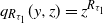$q_{R_{\tau_1}}(y,z)=z^{R_{\tau_1}}$ . Thus, (6.8) becomes

\begin{align*}y^m q_0(y,z) &= \mathbb{E}\big(y^{I_{\tau_1}} z^{R_{\tau_1}} [v(y,z)]^{A_{\tau_1}}\big)\\[3pt] &= p_1(z;\, m,l) + v(y,z) \big[\mathbb{E}\big(y^{I_{\tau_1}} z^{R_{\tau_1}}\big) - p_1(z;\, m,l)\big],\end{align*}

by arguing as for (2.12). We deduce that

\begin{equation*}\mathbb{E}\big(y^{I_{\tau_1}} z^{R_{\tau_1}}\big) = p_1(z;\, m,l) + \frac{y^mq_0(y,z)-p_1(z;\, m,l)}{v(y,z)},\end{equation*}

and substituting (2.6) for v(y, z) then gives the formula (6.6). Moreover, Proposition 2.2 directly yields the formula (6.7).

As a particular model, assume that the initial population has $I_0=1$ individual and the detection is activated only when $l=1$ individual has been removed. In this case, the state $ I_{\tau_1}$ still has a simple distributional representation. Define $\pi_1\in (0,1)$ again by the formula (2.18).

Corollary 6.1. Let $m=l=1$ . If positive, the population size $I_{\tau_1}$ is distributed as

(6.9) \begin{equation}(I_{\tau_1}\mid I_{\tau_1}\geq 1) \eqdist 1+G_1+ H_1,\end{equation}

where $G_1$ and $H_1$ are two independent geometric random variables of parameter $1-\pi_1$ and $\mu/(\mu+\lambda)$ , respectively.

Proof. From (6.6), (6.7) with $z=1$ , we have

\begin{equation*}\mathbb{E}\big(y^{I_{\tau_1}}\big) = p_1(1)q_0(p_1(1),1) - \frac{\alpha y\left[yq_0(y,1)-p_1(1)q_0(p_1(1),1)\right]}{\lambda y^2 - (\lambda+\mu+\alpha) y +\mu}.\end{equation*}

By factorizing the quadratic form as before in terms of $y_1(1)=p_1(1)$ and $y_2(1)=1/\pi_1$ , this can be rewritten as

(6.10) \begin{equation}\mathbb{E}\!\left(y^{I_{\tau_1}}\right) = p_1(1)q_0(p_1(1),1) + \frac{\alpha\pi_1}{\lambda}\frac{y}{1-\pi_1y} \, \frac{yq_0(y,1)-p_1(1)q_0(p_1(1),1)}{y-p_1(1)}.\end{equation}

Note from (6.2) that $yq_0(y,1) = \mu/[\mu+\lambda (1-y)]$ , so that

(6.11) \begin{align}yq_0(y,1)-p_1(1)q_0(p_1(1),1) &= \frac{\mu}{\mu+\lambda(1-p_1(1))} \frac{\lambda}{\mu+\lambda(1-y)} \,(y-p_1(1))\nonumber\\[3pt] &= \frac{p_1(1)q_0(p_1(1),1) y_3}{1-y_3y} \,(y-p_1(1)),\end{align}

in which we set $y_3=\lambda/(\mu+\lambda)$ $(<1)$ . Inserting (6.11) in (6.10), we obtain

\begin{align*}\mathbb{E}\!\left(y^{I_{\tau_1}}\right) &= p_1(1)q_0(p_1(1),1) + \frac{\alpha\pi_1}{\lambda} \frac{y}{1-\pi_1y} \, \frac{p_1(1)q_0(p_1(1),1)y_3}{1-y_3y}\\[3pt] &= p_1(1)q_0(p_1(1),1) p_1(1) + \frac{\alpha \pi_1 p_1(1)q_0(p_1(1),1)y_3}{\lambda (1-\pi_1)(1-y_3)} \, y \, \frac{1-\pi_1}{1-\pi_1y} \, \frac{1-y_3}{1-y_3y}\\[3pt] &= p_1(1)q_0(p_1(1),1) + [1-p_1(1)q_0(p_1(1),1)]\, y \, \frac{1-\pi_1}{1-\pi_1y} \, \frac{1-y_3}{1-y_3y},\end{align*}

where the last equality follows from the definitions of $\pi_1$ , $y_3$ , and $q_0(p_1(1),1)$ , and the fact that $p_1(1)$ is a root of (2.14). This implies the distributional representation (6.9) for $I_{\tau_1}$ under the condition that it is positive.

Second, we consider this time the case where $l>m$ , so that $R_{\tau_1}\geq m$ . Let us define the expectation $\phi_1(z;\, m,l)$ as

(6.12) \begin{equation}\phi_1(z;\, m,l) = \mathbb{E}\big(z^{R_{\tau_1}}\textbf{1}_{(I_{\tau_1}=0,R_{\tau_1}\geq l)}\big).\end{equation}

Proposition 6.2. If $l>m$ , the PGF of $(I_{\tau_1},R_{\tau_1})$ is given by

(6.13) \begin{equation}\mathbb{E}\!\left(y^{I_{\tau_1}}z^{R_{\tau_1}}\right) = \sum_{i=m}^{l-1} b_i z^i + \phi_1(z;\, m,l) - \frac{\alpha y[z^l h(y)-\phi_1(z;\, m,l)]}{\lambda y^2 - (\lambda+\mu+\alpha) y +\mu z},\end{equation}

where h(y) is defined by

\begin{equation*}h(y) = y^m\, \bigg[\frac{\mu}{y(\mu+\lambda(1-y))}\bigg]^l - \sum_{i=m}^{l-1} b_i \, \bigg[\frac{\mu}{y(\mu+\lambda(1-y))}\bigg]^{l-i},\end{equation*}

the $b_i$ are provided by (6.20) and (6.22) below, and $\phi_1(z;\, m,l)$ is given by

(6.14) \begin{equation}\phi_1(z;\, m,l) = z^l \, h\left(p_1(z)\right).\end{equation}

In particular, $I_{\tau_1}$ is of PGF

(6.15) \begin{equation}\mathbb{E}\!\left(y^{I_{\tau_1}}\right) = 1+h(1)-h\left(p_1(1)\right) - \frac{\alpha y[h(y)-h(p_1(1))]}{\lambda y^2 - (\lambda+\mu+\alpha) y +\mu }.\end{equation}

Proof. Stopping at time $\tau_1$ , we have

(6.16) \begin{align}y^m q_0 &= \mathbb{E}\big(y^{I_{\tau_1}} q_{R_{\tau_1}}(y,z) [v(y,z)]^{A_{\tau_1}}\big)\nonumber\\[3pt] &= \mathbb{E}\big(y^{I_{\tau_1}} z^{R_{\tau_1}} [v(y,z)]^{A_{\tau_1}} \textbf{1} _{(R_{\tau_1}\geq l)}\big)+ \mathbb{E}\big(y^{I_{\tau_1}} q_{R_{\tau_1}}(y,z) [v(y,z)]^{A_{\tau_1}}\textbf{1} _{(R_{\tau_1}<l)}\big)\nonumber\\[3pt] &= \mathbb{E}\big(y^{I_{\tau_1}} z^{R_{\tau_1}} [v(y,z)]^{A_{\tau_1}} \textbf{1} _{(R_{\tau_1}\geq l)}\big)+ \mathbb{E}\big(q_{R_{\tau_1}}(y,z)\textbf{1} _{(R_{\tau_1}<l)}\big),\end{align}

since $(R_{\tau_1}<l)$ implies that $A_{\tau_1}=0$ , hence $I_{\tau_1}=0$ too. Using (6.2) for $q_r(y,z)$ and setting $b_i\equiv \mathbb{P}(R_{\tau_1}=i)$ for $0\leq i\leq l-1$ , we obtain from (6.16) that

(6.17) \begin{multline}\mathbb{E}\big(y^{I_{\tau_1}} z^{R_{\tau_1}} [v(y,z)]^{A_{\tau_1}} \textbf{1} _{(R_{\tau_1}\geq l)}\big) \\= z^l \bigg\{y^m\, \bigg[\frac{\mu}{y(\mu+\lambda(1-y))}\bigg]^l - \sum_{i=0}^{l-1} b_i \, \bigg[\frac{\mu}{y(\mu+\lambda(1-y))}\bigg]^{l-i}\bigg\} \,\equiv\, z^l \, h(y), \mbox{ say}.\end{multline}

We are going to see how to determine the probabilities $b_i$ in (6.17). For that, we introduce an argument u by writing

(6.18) \begin{equation}u=y(\mu+\lambda(1-y)) . \end{equation}

Viewing (6.18) as a quadratic equation in y, we then get

\begin{equation*}y=\frac{1}{2\lambda} \{\lambda+\mu - [(\lambda+\mu)^2-4\lambda u]^{1/2}\} = \frac{\lambda+\mu}{2\lambda}\bigg\{1-\bigg[1-\frac{4\lambda u}{(\lambda+\mu)^2}\bigg]^{1/2}\bigg\}.\end{equation*}

Thus, y can be expanded under the form $\sum_{i=1}^{\infty} a_i u^i$ . As a result, we get

(6.19) \begin{equation}y^m=\Bigg(\sum_{i=1}^{\infty} a_i u^i\Bigg)^m=\sum_{i_1, \ldots, i_m\geq 1} a_{i_1} \cdots a_{i_m} u^{i_1+\cdots+i_m}=\sum_{k=m}^{\infty} c_k u^k,\end{equation}

where

(6.20) \begin{equation}c_k=\sum_{i_1,\ldots,i_m\geq 1\,: \, i_1+\cdots +i_m=k} a_{i_1} \cdots a_{i_m}.\end{equation}

Let us return to the right-hand side of (6.17). In terms of u, the function h(y) becomes, after insertion of (6.18) and (6.19), a function k(u) given by

(6.21) \begin{equation}k(u) = \Bigg(\sum_{k=m}^{\infty} c_k u^k\Bigg) \bigg(\frac{\mu}{u}\bigg)^l - \sum_{i=0}^{l-1} b_i \bigg(\frac{\mu}{u}\bigg)^{l-i}. \end{equation}

We note that the expectation on the left-hand side of (6.17) is bounded as $y \to 0$ . Thus, this is true for h(y) on the right-hand side. From (6.18), $y \to 0$ as $u \to 0$ , so that $k(u)\equiv h(y)$ must also be bounded when $u\to 0$ . But, from (6.21), k(u) can be expressed as

\begin{equation*}k(u) = \mu^l \Bigg(\sum_{k=m}^{l-1} \frac{c_k}{u^{l-k}}+ \sum_{k=l}^{\infty} c_k u^{k-l}\Bigg) - \Bigg(\sum_{i=0}^{m-1} \frac{\mu^{l-i} b_i}{u^{l-i}}+ \sum_{i=m}^{l-1} \frac{\mu^{l-i} b_i}{u^{l-i}}\Bigg).\end{equation*}

From this, we deduce that $b_0=b_1= \cdots =b_{m-1}=0$ (as we knew because $R_{\tau_1}\geq m$ ), and that the following $b_i$ are given by

(6.22) \begin{equation}b_i=\mu^i c_i, \qquad i=m, \ldots, l-1.\end{equation}

We can now derive the desired PGF. First, we rewrite the left-hand side of (6.17) taking into account that $I_{\tau_1}$ can be 0 or positive. This gives

(6.23) \begin{align}&\mathbb{E}\big(y^{I_{\tau_1}} z^{R_{\tau_1}} [v(y,z)]^{A_{\tau_1}} \textbf{1} _{(R_{\tau_1}\geq l)}\big) \nonumber\\[3pt] &\quad =\mathbb{E}\big(z^{R_{\tau_1}} \textbf{1}_{(I_{\tau_1}=0,R_{\tau_1}\geq l)}\big) + v(y,z) \mathbb{E}\big(y^{I_{\tau_1}} z^{R_{\tau_1}} \textbf{1}_{(I_{\tau_1}>0,R_{\tau_1}\geq l)}\big) \nonumber\\[3pt]& \quad =\phi_1(z;\, m,l) + v(y,z) \big[\mathbb{E}\big(y^{I_{\tau_1}} z^{R_{\tau_1}} \textbf{1}_{(R_{\tau_1}\geq l)}\big) - \phi_1(z;\, m,l)\big] \end{align}

in the notation of (6.12). Combining (6.17) and (6.23), we then obtain

\begin{equation*}\mathbb{E}\big(y^{I_{\tau_1}} z^{R_{\tau_1}} \textbf{1}_{(R_{\tau_1}\geq l)}\big) = \phi_1(z;\, m,l) + \frac{z^l h(y)-\phi_1(z;\, m,l)}{v(y,z)}.\end{equation*}

Thus, we find that $\phi_1(z;\, m,l)=z^l h(p_1(z))$ as stated in (6.14), and, using (2.6),

(6.24) \begin{equation}\mathbb{E}\big(y^{I_{\tau_1}} z^{R_{\tau_1}} \textbf{1}_{(R_{\tau_1}\geq l)}\big) = \phi_1(z;\, m,l) - \frac{\alpha y[z^l h(y)-\phi_1(z;\, m,l)]}{\lambda y^2 - (\lambda+\mu+\alpha) y +\mu z}.\end{equation}

On the other hand, we have

(6.25) \begin{equation}\mathbb{E}\big(y^{I_{\tau_1}} z^{R_{\tau_1}} \textbf{1}_{(R_{\tau_1}< l)}\big) = \mathbb{E}\big(z^{R_{\tau_1}} \textbf{1}_{(R_{\tau_1}< l)}\big) = \sum_{i=m}^{l-1} b_i z^i. \end{equation}

Therefore, adding the expectations (6.24), (6.25) yields the formula (6.13).

For $z=1$ , (6.14) becomes $\phi_1(1;\, m,l)=h(p_1(1))$ , and, from (6.13),

(6.26) \begin{equation}\mathbb{E}\!\left(y^{I_{\tau_1}}\right)=\sum_{i=m}^{l-1} b_i + h(p_1(1)) - \frac{\alpha y[h(y)-h(p_1(1))]}{\lambda y^2 - (\lambda+\mu+\alpha) y +\mu }.\end{equation}

Moreover, $\sum_{i=m}^{l-1} b_i = 1 - \mathbb{P}(R_{\tau_1}\geq l)$ by definition, and (6.24) for $y=z=1$ gives

(6.27) \begin{equation}\mathbb{P}(R_{\tau_1}\geq l) = \phi_1(1;\, m,l)-[h(1)-\phi_1(1;\, m,l)] = 2h(p_1(1))-h(1).\end{equation}

From (6.26) and (6.27), we deduce the formula (6.15) for the PGF of $I_{\tau_1}$ .

7. Alarms by recorded deaths

Until now, the individuals responsible for a possible alarm are those present in the population. In this section, we assume that the triggering of an alarm is due to the number of deaths that have occurred so far. Thus, the alarm rate in (1.1) is now given by $\alpha r$ (instead of $\alpha i$ ).

Let $t_0$ be any fixed moment. As in Section 5, our goal is to determine the PGF of the state $(I_{t_0}, R_{t_0}, A_{t_0})$ . Here too, there is no intervention after an alarm and $I_0=1$ . We try again a martingale like (5.1), i.e. of the form $M_t=f(I_t,R_t,A_t;\, t)$ for some bounded function f.

Lemma 7.1. $\{M_t,\, t\geq 0\}$ is a martingale if the functions $f(i,r,a;\, t)$ satisfy the differential equations

(7.1) \begin{align} &\frac{{\rm d} f(i,r,a;\, t)}{{\rm d} t} + \lambda i f(i+1,r,a;\, t) + \mu i f(i-1,r+1,a;\, t) + \alpha r f(i,r,a+1;\, t) \nonumber\\[3pt] & \quad = [(\lambda+\mu)i+\alpha r] f(i,r,a;\, t), \qquad i\geq 0.\end{align}

Let f be the function

(7.2) \begin{equation}f(i,r,a;\, t)=y(t)^i z(t)^r v^a,\end{equation}

where v is any real in (0, 1] and y(t), z(t) are functions of t in (0, 1]. Then, the equations (7.2) are satisfied if

(7.3) \begin{equation}z(t) = z_0 {\rm e}^{\alpha(1-v)(t-t_0)},\end{equation}

where $z(t_0)=z_0 \in [0,1]$ , and $y\equiv y(t)$ is the solution in (0, 1] of the Riccati equation

(7.4) \begin{equation}\frac{{\rm d} y}{{\rm d} t} + \lambda y^2 - (\lambda+\mu) y +\mu z_0 {\rm e}^{\alpha(1-v)(t-t_0)} = 0.\end{equation}

Proof. Arguing as for Lemma 5.1, we find this time that the $f(i,r,a;\, t)$ must satisfy the system of differential equations (7.1).

Choose now $f(i,r,a;\, t)$ of the special form (7.2). After simplification by $f(i,r,a;\, t)$ , these equations (7.1) are reduced to

(7.5) \begin{equation}i\bigg[\lambda y+\mu\frac{z}{y}-(\lambda+\mu)+\frac{{\rm d} y}{{\rm d} t}\frac{1}{y}\bigg] + r\bigg[\alpha(v-1) + \frac{{\rm d} z}{{\rm d} t}\frac{1}{z}\bigg] =0, \qquad i\geq 0.\end{equation}

Therefore, it suffices that the two terms $[\ldots]$ in (7.5) are equal to 0. The second condition yields the differential equation ${\rm d} z/{\rm d} t + \alpha(v-1)z =0$ . Its solution z(t), of value $z_0$ at time $t=t_0$ , is given by (7.3). The first condition yields the differential equation ${\rm d} y/{\rm d} t+\lambda y^2-(\lambda+\mu)y+\mu z=0$ , which is the Riccati equation (7.4) after inserting (7.3).

Let $y(t)\equiv y(t;\, t_0,y_0)$ , $t\geq 0$ , be the solution of the equation (7.4) that takes the value $y_0$ at the time $t=t_0$ , with $y_0$ arbitrary in [0,1]. Applying a standard method, we derive an explicit expression for this solution in Proposition A.3 of the appendix. Moreover, as desired, $y(t)\in (0,1]$ for $0\leq t \leq t_0$ . Obviously, y(t) depends here on the parameters $z_0,v$ . When $v=1$ , (7.4) becomes a Riccati equation with constant coefficients (as (5.4)).

From the martingale (5.1), (7.2), we then obtain

(7.6) \begin{equation}\mathbb{E}\big[y(t;\, t_0,y_0)^{I_t} z(t;\, t_0,z_0)^{R_t} v^{A_t}\big] = y(0; t_0,y_0), \qquad t\geq 0.\end{equation}

In particular, (7.6) at time $t=t_0$ gives

\begin{equation*} \mathbb{E}\big(y_0^{I_{t_0}} z_0^{R_{t_0}} v^{A_{t_0}}\big) = y(0; t_0,y_0),\end{equation*}

which is similar to the identity (5.12). Now, consider any stopping time (4.1). To obtain the desired PGF, we define a function $l(z_0,v)$ as in (5.7), then we follow the same reasoning as for Proposition 5.1. This leads to results with the same structure.

Appendix A. Technical results

We derive below some technical results used in proofs of Sections 4, 5, and 7.

A.1. Section 4

The following property allows us to establish the distributional representations (4.13) and (4.20).

Proposition A.1. Let $\xi$ be a random variable valued in $\mathbb{N}_0$ with PGF given by

(A.1) \begin{equation}\mathbb{E}(y^{\xi})= \frac{\sum_{i=0}^{k} b_i y^i}{(1-\delta y)^j}, \qquad y\in [0,1],\end{equation}

where j is a positive integer, k is a non-negative integer $<j$ , and $\delta$ is a real number in (0, 1). Then $\xi$ is distributed as a pseudo-mixture of sums of geometric random variables, i.e. its probability density function can be expressed as

(A.2) \begin{equation}\mathbb{P}(\xi=l) = \sum_{t=0}^{k} c_{j,t} \, \mathbb{P}(G_1+\cdots+ G_{j-t}=l), \qquad l\geq 0,\end{equation}

where $G_1, \ldots, G_{j}$ are i.i.d. geometric random variables of parameter $1-\delta$ , and the weights $c_{j,t}$ , which are not necessarily positive, are given by

(A.3) \begin{equation}c_{j,t} = (\!-1)^t (1-\delta)^{t-j} \, \sum_{i=t}^{k} {\left(\begin{array}{c}{i}\\{t}\end{array}\right)} \frac{b_i}{\delta^{i}}.\end{equation}

Proof. We write a monomial $y^i$ under the form

\begin{align*}y^i &= (1/\delta^{i}) (\delta y)^i = (1/\delta^{i}) (\delta y -1+1)^i\\[3pt] &= \frac{1}{\delta^{i}} \sum_{t=0}^{i} {\left(\begin{array}{c}{i}\\{t}\end{array}\right)} (\!-1)^t (1-\delta y)^t.\end{align*}

Dividing by $(1-\delta y)^j$ with $j>i $ $(\geq t)$ gives

\begin{align*}\frac{y^i}{(1-\delta y)^j} &= \frac{1}{\delta^{i}} \sum_{t=0}^{i} {\left(\begin{array}{c}{i}\\{t}\end{array}\right)} (\!-1)^t (1-\delta)^{t-j} \, \bigg(\frac{1-\delta}{1-\delta y}\bigg)^{j-t} \\[3pt] &= \frac{1}{\delta^{i}} \sum_{t=0}^{i} {\left(\begin{array}{c}{i}\\{t}\end{array}\right)} (\!-1)^t (1-\delta)^{t-j} \, \mathbb{E}\big(y^{G_1+\cdots+ G_{j-t}}\big),\end{align*}

where the random variables $G_j$ are defined as above. Thus, (A.1) can be rewritten as

\begin{eqnarray*}\mathbb{E}(y^{\xi}) &\,=\,& \sum_{i=0}^{k} \frac{b_i}{\delta^{i}} \sum_{t=0}^{i} {\left(\begin{array}{c}{i}\\{t}\end{array}\right)} (\!-1)^t (1-\delta)^{t-j} \, \mathbb{E}\big(y^{G_1+\cdots+ G_{j-t}}\big)\\ &\,=\,& \sum_{t=0}^{k} (\!-1)^t (1-\delta)^{t-j} \, \Bigg[\sum_{i=t}^{k} {\left(\begin{array}{c}{i}\\{t}\end{array}\right)} \frac{b_i}{\delta^{i}}\Bigg] \, \mathbb{E}\big(y^{G_1+\cdots+ G_{j-t}}\big).\end{eqnarray*}

In other words, $\xi$ is a mixture of $(k + 1)$ sums of geometrics, $G_1 + \cdots + G_{j-t}$ for $t = 0, \ldots, k$ , with weights $c_{j, t}$ given by (A.3), hence the formula (A.2). Note that the $c_{j, t}$ are not necessarily positive.

To illustrate the formula (4.13), we determine below the distribution of $(I_{\tau_j}\mid A_{\tau_j}=j)$ in the special cases $j=2,3,4$ .

A.1.1. Special cases of (4.13)

Let us return to the proof of this formula. For $j=2$ , we get from (4.16), (4.14) respectively

\begin{equation*}\chi_0(y) = \lim_{y\to 0}\, \frac{1}{y} \, \mathbb{E}\big(y^{I_{\tau_2}} \textbf{1}_{(A_{\tau_2}=2)}\big)= \frac{-\alpha w(0,1) p_{2,1}(1)}{[w(0,1)]^2} = \frac{\alpha}{\mu} p_{2,1}(1) \equiv \chi_0,\end{equation*}

since (4.15) gives $w(0,1)=-\lambda y_1(1)y_2(1)=-\mu$ . From (4.16), we have

\begin{equation*}\mathbb{E}\big(y^{I_{\tau_2}} \mid A_{\tau_2}=2\big) = y\, \frac{1}{p_{2,2}(1)}\,\frac{\chi_{0}}{(1-\pi_1 y)^2} =\bigg[\frac{\chi_0}{p_{2,2}(1)(1-\pi_1)^2}\bigg]\, y\, \frac{(1-\pi_1)^2}{(1-\pi_1 y)^2}.\end{equation*}

Taking $y=1$ shows that the constant $[\ldots]$ is equal to 1. Therefore, we deduce that $(I_{\tau_2}\mid A_{\tau_2}=2) \eqdist 1+G_1+G_2$ .

Consider $j=3$ and denote $\chi_1(y)=a_{1,0}+a_{1,1}y$ . From (4.16) and (4.14) we similarly obtain

\begin{equation*}a_{1,0} = \lim_{y\to 0}\, \frac{1}{y} \, \mathbb{E}\big(y^{I_{\tau_3}} \textbf{1}_{(A_{\tau_3}=3)}\big) = \frac{-\alpha [w(0,1)]^2 p_{3,2}(1)}{[w(0,1)]^3} = \frac{\alpha}{\mu} p_{3,2}(1).\end{equation*}

On the other hand, we also find that

\begin{align*}\lim_{y\to \infty}\, y \, \mathbb{E}\big(y^{I_{\tau_3}} \textbf{1}_{(A_{\tau_3}=3)}\big) &= \lim_{y\to \infty} \frac{y^2\,\chi_1(y)}{(1-\pi_1 y)^3}= \frac{a_{1,1}}{(\!-\pi_1)^3}\\[3pt] &= - \lim_{y\to \infty}\, \alpha^{3-2} \frac{[w(y,1)]^2}{[w(y,1)]^3} y^{3+1-2} p_{3,2}(1)= \frac{\alpha}{\lambda}p_{3,2}(1), \end{align*}

hence the value of $a_{1,1}$ . The expression of $\chi_1(y)$ follows. Using (4.17) and (A.2), we then deduce the representation (4.13); the details are omitted.

Consider $j=4$ and denote $\chi_2(y)=a_{2,0}+a_{2,1}y+a_{2,2}y^2$ . As for $j=3$ , we take successively $y\to 0$ and $y\to \infty$ to obtain

\begin{align*}\lim_{y\to 0}\, \frac{1}{y} \, \mathbb{E}\big(y^{I_{\tau_4}} \textbf{1}_{(A_{\tau_4}=4)}\big) & = a_{2,0} = \frac{\alpha}{\mu} p_{4,3}(1), \\[3pt] \lim_{y\to \infty}\, \frac{y^2\chi_2(y)}{(1-\pi_1y)^4} & = \frac{a_{2,2}}{\pi_1^4}= \lim_{y\to \infty}\, y \, \mathbb{E}\big(y^{I_{\tau_4}} \textbf{1}_{(A_{\tau_4}=4)}\big)\\[3pt] & = - \lim_{y\to \infty}\, \alpha^{4-3} \frac{[w(y,1)]^3}{[w(y,1)]^4} y^{4+1-3} p_{4,3}(1) = \frac{\alpha}{\lambda} p_{4,3}(1),\end{align*}

which gives us $a_{2,2}$ . Moreover, when $y=1$ , we have

\begin{equation*}\chi_2(1) = a_{2,0}+a_{2,1}+a_{2,2} = (1-\pi_1)^4 p_{4,4}(1),\end{equation*}

the last equality resulting from (4.16). This gives $a_ {2,1}$ and so $\chi_2( y) $ , hence again (4.13).

Remark A.1. The polynomial $\chi_{j-2}(y)$ can also be determined once its derivatives at $y=0$ are known. From (4.16) and (4.14), we see that

\begin{equation*}\chi_{j-2}(y) = (1-\pi_1 y)^j \bigg\{\alpha^j y^{j} [w(y,1)]^{-j} - \sum_{a=0}^{j-1} \alpha^{j-a} [w(y,1)]^{a-j} y^{j-1-a} p_{j,a}(1)\bigg\}.\end{equation*}

Thus, the calculation of the derivatives $[\chi_{j-2}(y)]^{(i)}$ requires calculating the derivatives $[w(y,1)^b]^{(k)}$ (with b a negative integer) for $1\leq i,k \leq j-2$ . As w(y,1) is a polynomial of degree 2, we obtain

\begin{equation*}[w(y,1)^b]^{(k)} = \sum_{r=0}^{[k/2]} c_{k,r}\, b_{[k-r]} [w(y,1)]^{b-k+r} \big[w(y,1)^{(1)}\big]^{k-2r} \big[w(y,1)^{(2)}\big]^{r},\end{equation*}

where the coefficients $c_{k,r}$ satisfy the recurrence

\begin{equation*}c_{k,0} = 1, \qquad c_{k+1,r} = c_{k,r} + (k+2-2r) c_{k,r-1}, \qquad k\geq 1, \, 1\leq r \leq [k/2].\end{equation*}

A.2. Section 5

For Proposition 5.1, we must know the function l(z, v) given by (5.7), and thus the values of $y(0; t_0, y_0)$ and $y(0; t_0, 0)$ . These are provided by the solution $y(t)=y(t;\, t_0,y_0)$ of the Riccati equation (5.4), with constant coefficients, satisfying $y(t_0; t_0,y_0)=y_0\in [0,1]$ . Let us derive that solution.

Proposition A.2. The solution of the Riccati equation (5.4) is

(A.4) \begin{equation}y(t;\, t_0,y_0)=c+m+\frac{2m(y_0-c-m)}{(y_0-c+m)\exp(2m\lambda (t-t_0))-(y_0-c-m)},\end{equation}

where $c\equiv c(v)$ and $m\equiv m(z,v)$ are defined by

(A.5) \begin{equation}c= \frac{\lambda+\mu+\alpha(1-v)}{2\lambda}, \qquad m=\bigg(c^2 -\frac{\mu z}{\lambda}\bigg)^{1/2},\end{equation}

with $m>0$ for z small enough. This solution is such that $y(t;\, t_0,y_0)\in [0,1]$ for all $0\leq t \leq t_0$ .

Proof. Equation (5.4) can be rewritten as

\begin{equation*}- \frac{{\rm d} y}{{\rm d} t} =\lambda \bigg[y-\frac{\lambda+\mu+\alpha(1-v)}{2\lambda}\bigg]^2 - \bigg[\frac{(\lambda+\mu+\alpha(1-v))^2}{4\lambda} -\mu z\bigg] = \lambda [(y-c)^2 - m^2] \end{equation*}

using the notation (A.5). Setting $\bar y\equiv y-c$ , that equation just becomes ${\rm d} \bar y/ (\bar y^2 -m^2) = -\lambda {\rm d} t$ . At time $t_0$ we have $\bar y_0=y_0-c$ by assumption. After some calculations, we then obtain as a solution

\begin{equation*}\frac{\bar y+m}{\bar y-m} = \frac{\bar y_0+m}{\bar y_0-m} {\rm e}^{2m\lambda (t-t_0)}.\end{equation*}

The left-hand side is equal to $1+2m/(\bar y-m)$ , so that

\begin{equation*}\bar y = m+ \frac{2m(\bar y_0-m)}{(\bar y_0+m)\exp[2m\lambda (t-t_0)] - (\bar y_0-m)}.\end{equation*}

This becomes the formula (A.4) for $y=y(t;_0,y_0)$ .

It remains to show that $y(t;\, t_0,y_0)$ of value $y_0\in [0,1]$ at time $t=t_0$ stays in the interval [0,1] when we go back in time from $t_0$ to 0. Let us prove this by contradiction. A first possibility would be to go through the point 0 at some time $t_1$ ( $<t_0$ ). Then, $y(t_1)=0$ and, from (5.4), this implies that ${\rm d} y/{\rm d} t<0$ at time $t_1$ , which is contradictory (remember that we work in reverse time from $t_0$ to 0). A second posibility would be to go through the point 1 at some time $t_2$ ( $<t_0$ ). Then, $y(t_2)=1$ and, from (5.4), we see that ${\rm d} y/{\rm d} t>0$ at time $t_2$ , which is again contradictory.

A.3. Section 7

Proposition 7.1 is expressed similarly in terms of the function $l(z_0,v)$ . Thus, to compute the values of $y(0; t_0, y_0)$ and $y(0; t_0, 0)$ , we must obtain the solution $y(t)=y(t;\, t_0,y_0)$ of the Riccati equation (7.4) satisfying $y(t_0; t_0,y_0)=y_0\in [0,1]$ . To get it, we start with a brief reminder.

Lemma A.1. The confluent hypergeometric equation

\begin{equation*}x\frac{{\rm d}^2y}{{\rm d} x^2} + (\gamma-x) \frac{{\rm d} y}{{\rm d} x} -\alpha y =0 \end{equation*}

admits, if $\gamma$ is not an integer, the linearly independent solutions

\begin{equation*}F(\alpha, \gamma;\, x) = \sum_{n=0}^\infty \prod_{j=0}^{n-1}\frac{\alpha+j}{\gamma+j}\frac{x^n}{n!} \quad \text{and} \quad x^{1-\gamma} F(\alpha-\gamma+1, 2-\gamma;\, x),\end{equation*}

called confluent hypergeometric functions of the first and second kinds.

From this lemma, we deduce that the equation

(A.6) \begin{equation}x\frac{{\rm d}^2y}{{\rm d} x^2} + \gamma \frac{{\rm d} y}{{\rm d} x} -\alpha y =0 \end{equation}

admits the linearly independent solutions

(A.7) \begin{align}& G(\alpha, \gamma;\,x) = \lim_{k\to 0}F(\alpha/k, \gamma;\, kx) = \sum_{n=0}^\infty \frac{\alpha^n}{\prod_{j=0}^{n-1}(\gamma+j)}\frac{x^n}{n!},\nonumber\\[3pt] & H(\alpha, 2-\gamma;\,x) = \lim_{k\to 0} x^{1-\gamma} F(\alpha/k-\gamma+1, 2-\gamma;\, kx) = x^{1-\gamma} G(\alpha, 2-\gamma;\,x).\end{align}

Now, consider the Riccati equation (7.4). We define the constants $\rho, a, b$ as

(A.8) \begin{equation}\rho=\alpha (1-v), \qquad b=-(\lambda+\mu)/\rho, \qquad c=\lambda \mu z_0 {\rm e}^{-\rho t_0}/\rho^2,\end{equation}

so that (7.4) takes the form

(A.9) \begin{equation}\frac{{\rm d} y}{{\rm d} t} + \lambda y^2 +b\rho y + \frac{c}{\lambda}\rho^2 {\rm e}^{\rho t}= 0.\end{equation}

Proposition A.3. The solution of the Riccati equation (A.9) is

(A.10) \begin{equation}y(t ; t_0, y_0) = \frac{\rho\tau}{\lambda}\, \frac{c_0 ({\rm d}/{\rm d}\tau) G(\!-c,b+1;\, \tau) + ({\rm d}/{\rm d}\tau) H(\!-c, 1-b;\, \tau)}{c_0 G(\!-c,b+1;\, \tau) + H(\!-c, 1-b;\, \tau)},\end{equation}

where $\tau\equiv\exp(\rho t)$ , G, H are defined in (A.7), and $c_0$ is the constant

(A.11) \begin{equation}c_0 = \frac{\rho \tau_0 [({\rm d}/{\rm d}\tau)H(\!-c, 1-b;\, \tau)]_{\tau=\tau_0} - \lambda y_0 H(\!-c, 1-b;\, \tau_0)}{\lambda y_0G(\!-c,b+1;\, \tau_0)-[({\rm d}/{\rm d}\tau)G(\!-c,b+1;\, \tau)]_{\tau=\tau_0}}.\end{equation}

This solution is such that $y(t;t_0,y_0)\in [0,1]$ for all $0\leq t \leq t_0$ .

Proof. Let $u(t)\equiv \exp(\lambda\int_0^t y(s){\rm d} s)$ , so that ${\rm d} u/{\rm d} t=\lambda y u$ . After multiplication by $\lambda u$ , (A.9) can be rewritten as

(A.12) \begin{equation}\frac{{\rm d}^2u}{{\rm d} t^2} + b\rho \frac{{\rm d} u}{{\rm d} t} + c\rho^2 {\rm e}^{\rho t} u=0.\end{equation}

Put $\tau=\exp(\rho t)$ as announced, and then denote $u(t)\equiv v(\tau)$ . Obviously, ${\rm d} u/{\rm d} t=({\rm d} v/{\rm d}\tau) \rho\tau$ and ${\rm d}^2u/{\rm d} t^2=({\rm d}^2v/{\rm d}\tau^2) \rho^2\tau^2+({\rm d} v/{\rm d}\tau) \rho^2\tau$ . Therefore, (A.12) becomes, after simplification by $\rho^2 \tau$ , the second-order linear differential equation

\begin{equation*}\tau \frac{{\rm d}^2v}{{\rm d}\tau^2} + (b+1) \frac{{\rm d} v}{{\rm d}\tau} + cv =0,\end{equation*}

which is exactly of the type (A.6). From (A.7), the general solution of this equation is

(A.13) \begin{equation}v(\tau) = c_1 G(\!-c,b+1;\, \tau) + c_2H(\!-c, 1-b;\, \tau) \end{equation}

for some constants $c_1, c_2$ . By the definition of u(t) and $v(\tau)$ ,

\begin{equation*}y(t;\, t_0, y_0) = \frac{1}{\lambda}\, \frac{{\rm d} u(t)}{{\rm d} t}\frac{1}{u(t)} = \frac{\rho\tau}{\lambda}\,\frac{{\rm d} v(\tau)}{{\rm d} \tau}\frac{1}{v(\tau)},\end{equation*}

and, using (A.13), we then deduce the formula (A.10) in which $c_0\equiv c_1/c_2$ . This constant $c_0$ is such that $y(t)=y_0$ at time $t_0$ , i.e. when $\tau_0=\exp(\rho t_0)$ , hence its expression (A.11). Finally, as for Proposition A.2, we obtain from (7.4) that $y(t;\,t_0,y_0)$ of value $y_0\in [0,1]$ at $t_0$ stays in the interval [0,1] for $0\leq t \leq t_0$ .