2.1. Control set-up

This study focuses on the transonic buffet flow over the NACA 0012 aerofoil. The active control actuator is a trailing-edge flap with a length of $15\,\%$ chord and its rotation axis located at $85\,\%$ chord length, as shown in figure 1. Compared with TED, the trailing-edge flap is the original control surface of the wing, eliminating the need to add any additional devices to the system and thereby simplifying the modelling procedure. The closed-loop control takes lift coefficient as the feedback signal. $u_\infty$ represents the free-stream velocity, $x_F$ represents the position of the rotation axis of the trailing edge flap and $c$ is the chord length of the airfoil. As figure 1 illustrates, $\alpha$ is the angle of attack representing the angle between the direction of incoming flow and the chord of the aerofoil, and $\beta$ is the flap deflection angle showing the angle between the deflected flap and the chord of the aerofoil. The value of $\alpha$ is decided by incoming flow conditions and  $\beta$ is determined by closed-loop control law.

Figure 1.

Sketch diagram of NACA 0012 aerofoil and control system.

2.2. CFD simulation

The numerical simulation of transonic buffet flow is conducted using an in-house hybrid-unstructured flow solver. The finite-volume method is employed to solve the unsteady Reynolds-averaged Navier–Stokes (URANS) equations. The Spalart–Allmaras (SA) turbulence model is applied to close the URANS equations for two-dimensional compressible flow.

The spatial discretisation and time integration of the turbulence model equation and the mean flow equations are weakly coupled. The inviscid flux is discretised by the second-order advection upstream splitting method (AUSM+) and least-squares reconstruction scheme. And the viscous flux is evaluated by the second-order central scheme. The time discretisation uses the dual time stepping method while the pseudo time iteration applies the fourth-stage Runge–Kutta scheme. A detailed introduction to this study’s numerical method can be found in Appendix A and Gao et al. (Reference Gao, Zhang and Ye2016).

Figure 2 shows the hybrid computational domain of the NACA 0012 aerofoil employed in this study, which is the same as G3 in Gao et al. (Reference Gao, Zhang and Ye2016). The far field extends 20 chords from the aerofoil. There are 25 361 surface nodes and 50 layers of the structured viscous grid around the aerofoil. The height of the first boundary layer near the wall is $5 \times 10^{-6}c$ (where $c$ denotes the chord length of the aerofoil), and the non-dimensional wall distance is $y^+\lt 1$ . The simulation real-time step is $dt_{\textit{real}}=2.94 \times 10^{-4}\,\rm s$ (physical) and the non-dimensional time step is $dt=dt_{\textit{real}}\times a/c=0.1$ , where $a$ represents the velocity of sound. The chosen Reynolds number throughout this article is $Re=3 \times 10^{6}$ . 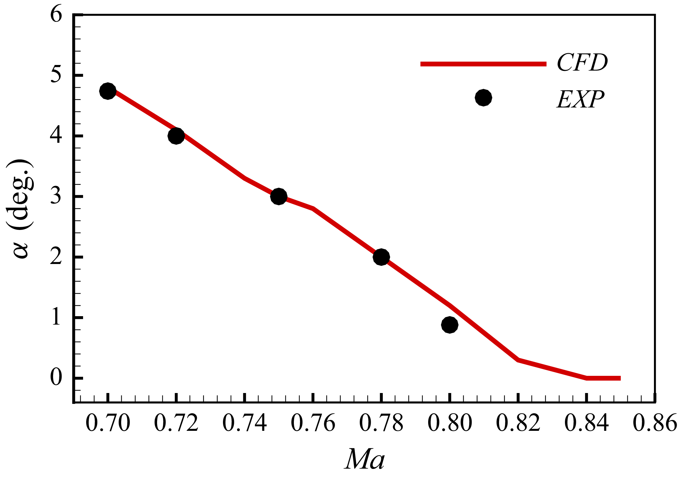As figure 3 shows, the calculated buffet-onset boundary is in good agreement with the experimental results (Doerffer et al. Reference Doerffer, Hirsch, Dussauge, Babinsky and Barakos2010). For instance, the simulated buffet-onset angle of attack is approximately $4.8^{\circ }$ when ${\textit{Ma}}=0.7$ , which is basically consistent with the experimental value of $4.74^{\circ }$ . Under this Mach number, the maximum buffet load is obtained at an attack angle of $5.5^{\circ }$ . Figure 4 shows the lift coefficient response developing from the unstable steady state to nonlinear limit cycle state and corresponding spectral analysis at ${\textit{Ma}}=0.7$ , $\alpha =5.5^{\circ }$ . The intrinsic Strouhal frequency of the system under this condition is $St=\textit{fc}/u_{\infty }=0.062$ , where $f$ is the flow frequency and $u_{\infty }$ is the free-stream velocity.

Figure 2.

(a) Overview of the NACA 0012 aerofoil computational grid and (b) detailed mesh around the aerofoil. X, Y here represent the dimensionless x and y coordinates.

Figure 3.

Comparison of buffet-onset boundary.

Figure 4.

(a) Lift response and (b) the wavelet analysis of it at ${\textit{Ma}}=0.7$ , $\alpha =5.5^{\circ }$ . $C_l$ is the lift coefficient, and $A$ is the amplitude of the wavelet coefficient reflecting the degree of similarity or resonance intensity between the original signal and the wavelet basis function at a specific time and frequency.

2.3. Flow characteristics

This section examines the time-varying characteristics of the transonic buffet flow under an incoming flow condition when the angle of attack $\alpha$ varies from $4.0^\circ$ to $5.5^\circ$ while the Mach number remains constant at 0.70, as illustrated in figure 5(a). Through the aforementioned numerical simulation method, the aerodynamic responses of the NACA 0012 aerofoil are obtained, such as the lift coefficient response depicted in figure 5(b). Figure 5(c) further shows the variation patterns of the dominant frequency of the lift coefficient response under this changing flow condition. The grey area in the figure represents the buffet region. It can be concluded that, as the angle of attack $\alpha$ increases from the non-buffet stage to the buffet stage, the fluctuation amplitude of the aerodynamic response will rise rapidly, and the response frequency will also experience a continuous increase. Moreover, a premature buffet phenomenon may occur attributable to the disturbance caused by the changing condition.

Figure 5.

The time-varying characteristics of the transonic buffet flow when ${\textit{Ma}}=0.70$ , $\alpha =4.0^\circ \sim 5.5^{\circ }$ : (a) the time-variant incoming flow condition; (b) the calculated lift coefficient response and (c) the wavelet analysis of the time-varying response.

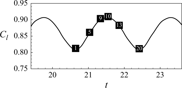
Furthermore, six typical time intervals are selected for conducting DMD modal analysis. The central moments of these intervals are illustrated as red circles in figure 5(b) and labelled in chronological sequence. The first three DMD modes, ranked by modal energy, are presented in figure 6, accompanied by the corresponding pressure fields at the representative moments. As observed in figure 6(a), the position of the leading shock wave shifts progressively from $P_s=0.314$ to $P_s=0.158$ over time, where $P_s=x_s/c$ and $x_s$ represents the chordwise coordinate of the shock wave. The first-order DMD mode corresponds to the zero-frequency time-averaged static mode, whose edge becomes increasingly indistinct, indicating that the flow field undergoes more pronounced variations as time progresses. The remaining modes capture the dynamic features associated with oscillating shock waves. Specifically, the second-order DMD modal frequency gradually converges towards the natural frequency $St=0.063$ of the transonic buffet flow at ${\textit{Ma}}=0.70$ and $\alpha =5.5^\circ$ , starting from an initial value of $St=0.014$ . Meanwhile, the third-order mode emerges as a harmonic mode of the second-order mode. This observation indicates that the second-order DMD mode corresponds to the main mode of oscillatory shock waves, gradually dominating the transonic buffet flow characteristics over time.

Figure 6.

Pressure fields of the time-varying transonic buffet flow and the top three DMD pressure modes at typical moments. $C_p$ here represents the pressure coefficient.

These results strongly demonstrate the sensitivity of the intrinsic characteristics of transonic buffet flow over aerofoils to changes in incoming flow conditions. Meanwhile, the strong nonlinearity of the change in the intrinsic features puts higher demands on the accuracy of aerodynamic modelling and control effectiveness under time-variant incoming flow conditions. Therefore, it is necessary to develop time-variant modelling methods and control design methods for transonic buffet flow under changing conditions.

2.4. Adaptive control design framework

The primary existing approach to establishing TV-ROMs is the ‘evolve then correct’ methodology, where a basic flow evolution model is first established, followed by the development of an error model that captures the discrepancy between time series simulation and the basic model prediction through methods such as neural networks. For example, Pawar et al. (Reference Pawar, Ahmed, San and Rasheed2020) employed a recurrent neural network to correct the original intrusive Galerkin model in real time, greatly improving the prediction accuracy of the model. However, the error models introduced to augment model precision often incorporate strong nonlinear terms that are difficult to explicitly represent, posing unpredictable challenges for control design research.

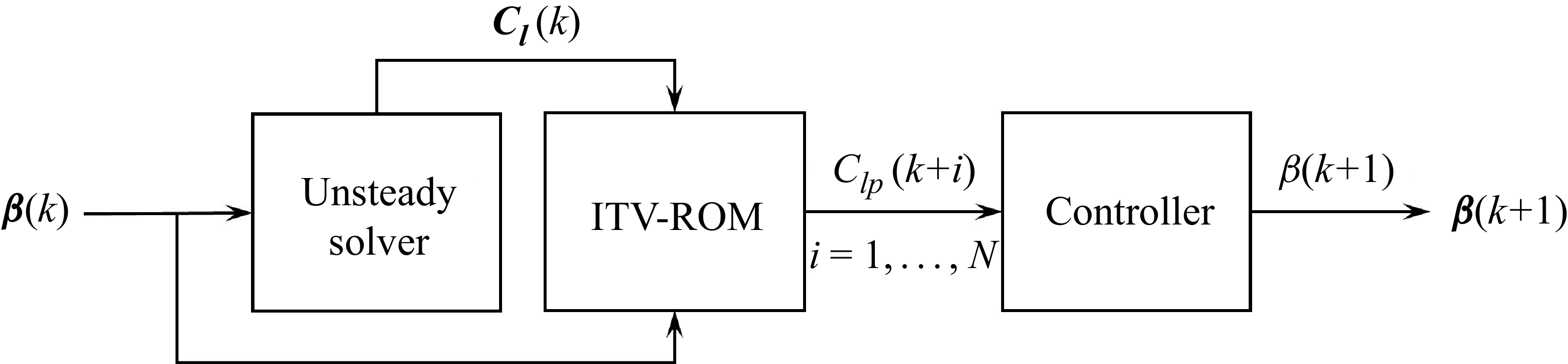
To avoid introducing additional nonlinear terms for error correction, this article develops an ITV-ROM method rooted in the traditional time-invariant modelling architecture, and combines it with adaptive controllers to achieve superior suppression of transonic buffet under time-variant conditions. The parameter update process for time-variant modelling and adaptive control design is shown in figure 7. The data required for updating the parameters of TV-ROMs are the deflection history $\boldsymbol{\beta }(k)=[\beta (k{-}i),\beta (k-i+1),\ldots ,\beta (k)]^{\mathrm{T}}$ of the trailing-edge flap from time step $(k-i)$ to current time step $k$ and the lift response $\boldsymbol{C_l}(k)=[C_l(k-i),C_l(k-i+1),\ldots ,C_l(k)]^{\mathrm{T}}$ of the flow system under control. Subsequently, the lift response $C_{lp}(k+i), (i=1,\ldots ,N)$ at time step $(k+i)$ is predicted by the updated model as the input of the adaptive controller. Then the flap deflection angle at the next time step $\beta (k+1)$ is determined by the controller, and the subsequent lift response is calculated using an unsteady CFD solver. By following this process, the adaptive control law design for time-variant flow conditions can be readily achieved.

Figure 7.

Combination of time-variant modelling and adaptive control design.

The two self-tuning control design methods adopted in this article are minimum variance control (MVC) and GPC. The detailed adaptive control design framework is shown in figure 8. The whole design procedure consists of two circuits, which are inner loop A and outer loop B. The inner loop A is composed of a flow system to be controlled and an adjustable controller. The control law generated by the controller acts directly on the flow system. This set-up is quite similar to the traditional feedback loop commonly employed in closed-loop control system. The outer loop B comprises the identification of the ITV-ROM’s parameters and the update of the self-tuning controller’s parameters, which is the core component of our adaptive control design framework. In this way, the proposed ITV-ROM parameter identification and controller adjustment processes are combined organically to form a real-time control system, thus achieving adaptive control under time-variant incoming flow conditions.

Figure 8.

The adaptive control design framework.

3.1. Traditional time-invariant ARX modelling approach

The ARX model is usually used to build the aerodynamic ROM (Shi et al. Reference Shi, Gao, Liu and Zhang2025), which establishes the transfer function relationship between the input and output data of a complex system based on the following single-input single-output difference equations:

(3.1) \begin{equation} y(k) = \sum \limits _{i = 1}^{na} {{{A}_i}y(k - i)} + \sum \limits _{i = d}^{nb} {{{B}_i}u(k - i)} + \xi (k). \end{equation}

For this study, $u(k)$ in (3.1) represents the control input, namely, the actuation displacement $\beta (k)$ of the trailing-edge flap; $y(k)$ is the numerical simulated aerodynamic response $f_a$ , such as lift coefficient response $C_l$ , also serving as the feedback signal; and $\xi (k)$ refers to the white noise sequence. Both the input and output data are obtained completely before modelling in this part of work. Here $A_i$ and $B_i$ are the coefficients to be identified offline, where $na$ and $nb$ are the delay orders of the input and output datasets and $d$ is the pure delay between the input and output data, which is taken as $d=0$ in this study.

Usually, the coefficients are identified through the least-squares (LS) method. Define the parameter matrix $\boldsymbol{\theta }$ and the state vector ${{\boldsymbol{x}}}(k)$ as follows:

(3.2) \begin{equation} \begin{aligned} \boldsymbol{\theta }&=\begin{bmatrix}A_1,&{\cdots} ,&A_{na},&B_d,&{\cdots} ,&B_{nb}\end{bmatrix}^{\mathrm{T}},\\ \boldsymbol{x}(k)&=\begin{bmatrix}y(k-1),&{\cdots} ,&y(k-na),&u(k-d),&{\cdots} ,&u(k-nb)\end{bmatrix}^{\mathrm{T}}. \end{aligned} \end{equation}

Then (3.1) can be rewritten as

(3.3) \begin{equation} y(k)=\boldsymbol{x}^{\mathrm{T}}(k)\boldsymbol{\theta }+\xi (k). \end{equation}

Assume that there are $L$ couples of input/output data $\{y(k), u(k), k=1,2,\ldots ,L, L\gt (na+nb-d+1)\}$ , then the target of the parameter identification process is to minimise the LS criterion $\textit {J}$ :

(3.4) \begin{equation} \begin{aligned} \textit {J}=\sum _{k=1}^{L}\xi ^{2}(k)=\sum _{k=1}^{L}\left[y(k)-\boldsymbol{x}^{\mathrm{T}}(k)\boldsymbol{\tilde {\theta }}\right]^{2}, \end{aligned} \end{equation}

where $\boldsymbol{\tilde {\theta }}=\begin{bmatrix}\tilde {A}_1,&\!{\cdots} ,&\!\tilde {A}_{na},&\!\tilde {B}_d,&\!{\cdots} ,&\!\tilde {B}_{nb}\end{bmatrix}^{\mathrm{T}}$ represents the identified parameter vector.

Further define the following vectors:

(3.5) \begin{align} \begin{array}{l} \boldsymbol{Y}=\begin{bmatrix}y(1),&y(2),&{\cdots} ,&y(L)\end{bmatrix}^{\mathrm{T}} \in \mathbb{R}^{L \times 1},\\ \boldsymbol{E}=\begin{bmatrix}\xi (1),&\xi (2),&{\cdots} ,&\xi (L)\end{bmatrix}^{\mathrm{T}} \in \mathbb{R}^{L \times 1},\\ \boldsymbol{\varPhi }^{\mathrm{T}}=\begin{bmatrix}\boldsymbol{x}(1),&\boldsymbol{x}(2),&{\cdots} ,&\boldsymbol{x}(L)\end{bmatrix} \in \mathbb{R}^{(na+nb-d+1) \times L}. \end{array} \end{align}

Then (3.4) can be turned into

(3.6) \begin{equation} \begin{aligned} \textit {J}&=\boldsymbol{E}^{\mathrm{T}}\boldsymbol{E}\\ &=(\boldsymbol{Y}-\boldsymbol{\varPhi }\boldsymbol{\tilde {\theta }})^{\mathrm{T}}(\boldsymbol{Y}-\boldsymbol{\varPhi }\boldsymbol{\tilde {\theta }})\\ &=\boldsymbol{Y}^{\mathrm{T}}\boldsymbol{Y}-2(\boldsymbol{\varPhi }^{\mathrm{T}}\boldsymbol{Y})^{\mathrm{T}}\boldsymbol{\tilde {\theta }}+\boldsymbol{\tilde {\theta }}^{\mathrm{T}}\boldsymbol{\varPhi }^{\mathrm{T}}\boldsymbol{\varPhi }\boldsymbol{\tilde {\theta }}. \end{aligned} \end{equation}

Make the first derivative of $\textit {J}$ with respect to $\boldsymbol{\tilde {\theta }}$ equal to 0:

(3.7) \begin{equation} \begin{aligned} \frac {\partial J}{\partial \tilde {\boldsymbol{\theta }}}=-2\boldsymbol{\varPhi }^{\mathrm{T}}\boldsymbol{Y}+2\boldsymbol{\varPhi }^{\mathrm{T}}\boldsymbol{\varPhi }\tilde {\boldsymbol{\theta }}=0. \end{aligned} \end{equation}

Finally, the parameter vector $\tilde {\boldsymbol{\theta }}$ identified through the LS method is shown as follows:

(3.8) \begin{equation} \begin{aligned} \tilde {\boldsymbol{\theta }}=[\boldsymbol{\varPhi }^{\mathrm{T}}\boldsymbol{\varPhi }]^{-1}\boldsymbol{\varPhi }^{\mathrm{T}}\boldsymbol{Y}, \end{aligned} \end{equation}

where $\boldsymbol{\varPhi }$ should be a full column-rank matrix, which requires non-zero input and output data.

Notably, the establishment of (3.1) is based on the assumption that the input and output data of the system satisfy the linear superposition principle. This requires that the acquisition process of the input/output data for linear modelling the transonic buffet system should be constrained within the linear developing stage, imposing stringent requirements on the design of the training signal which serves as both the input data and the external excitation for generating the corresponding output data (Dou et al. Reference Dou, Gao and Zhang2024).

The established ARX model can accurately model the overall dynamic characteristics of the system and be easily changed into discrete state space equations with the help of the state vector ${{\boldsymbol{x}}}(k)$ as follows:

(3.9) \begin{equation} \left \{ \!\!\begin{array}{l} \boldsymbol{x}(k+1)={\tilde {\boldsymbol{A}}}\boldsymbol{x}(k)+{\tilde {\boldsymbol{B}}}u(k-d),\\ y(k)={\tilde {\boldsymbol{C}}}\boldsymbol{x}(k)+{\tilde {B}_d}u(k-d), \end{array} \right . \end{equation}

where

(3.10) \begin{align} \begin{array}{l} {\tilde {\boldsymbol{A}}} = \left [ {\begin{array}{*{20}{c}} {\tilde {A}_1}&{\tilde {A}_2}& {\cdots} &{\tilde {A}_{na - 1}}&{\tilde {A}_{na}}&{0}&{\tilde {B}_{d+1}}&{\tilde {B}_{d+2}}& {\cdots} &{\tilde {B}_{nb - 1}}&{\tilde {B}_{nb}}\\ {1}&{0}& {\cdots} &{0}&{0}&{0}&{0}&{0}& {\cdots} &{0}&{0}\\ \vdots &{1}& {\cdots} &{0}&{0}&{0}&{0}&{0}& {\cdots} &{0}&{0}\\ \vdots & \vdots & \ddots & \vdots & \vdots & \vdots & \vdots & \vdots & \ddots & \vdots & \vdots \\ {0}&{0}& {\cdots} &{1}&{0}&{0}&{0}&{0}& {\cdots} &{0}&{0}\\ {0}&{0}& {\cdots} &{0}&{1}&{0}&{0}&{0}& {\cdots} &{0}&{0}\\ {0}&{0}& {\cdots} &{0}&{0}&{0}&{0}&{0}& {\cdots} &{0}&{0}\\ {0}&{0}& {\cdots} &{0}&{0}&{0}&{1}&{0}& {\cdots} &{0}&{0}\\ {0}&{0}& {\cdots} &{0}&{0}&{0}&{0}&{1}& {\cdots} &{0}&{0}\\ \vdots & \vdots & \ddots & \vdots & \vdots & \vdots & \vdots & \vdots & \ddots & \vdots & \vdots \\ {0}&{0}& {\cdots} &{0}&{0}&{0}&{0}&{0}& {\cdots} &{1}&{0} \end{array}} \right ]\!,\\ {\tilde {\boldsymbol{B}}} = \left [ {\begin{array}{*{20}{c}} {\tilde {B}_d}&{0}&{{\cdots} }&{0}&{1}&{0}&{0}&{{\cdots} }&{0} \end{array}} \right ]^{\mathrm{T}}\!,\\ {\tilde {\boldsymbol{C}}} = \left [ {\begin{array}{*{20}{c}} {\tilde {A}_1}&{\tilde {A}_2}& {\cdots} &{\tilde {A}_{na - 1}}&{\tilde {A}_{na}}& {0} &{\tilde {B}_{d+1}}&{\tilde {B}_{d+2}}& {\cdots} &{\tilde {B}_{nb - 1}}&{\tilde {B}_{nb}} \end{array}} \right ]\!.\\ \end{array} \end{align}

Subsequently, the discrete-time form equations can be further turned into the continuous-time form shown through bilinear transformation as follows:

(3.11) \begin{equation} \left \{ \begin{array}{l} \dot {\boldsymbol{x}}(t)={\boldsymbol{A}}\boldsymbol{x}(t)+\boldsymbol{B}u(t-t_0),\\ y(t)=\boldsymbol{C}\boldsymbol{x}(t)+B_du(t-t_0). \end{array} \right . \end{equation}

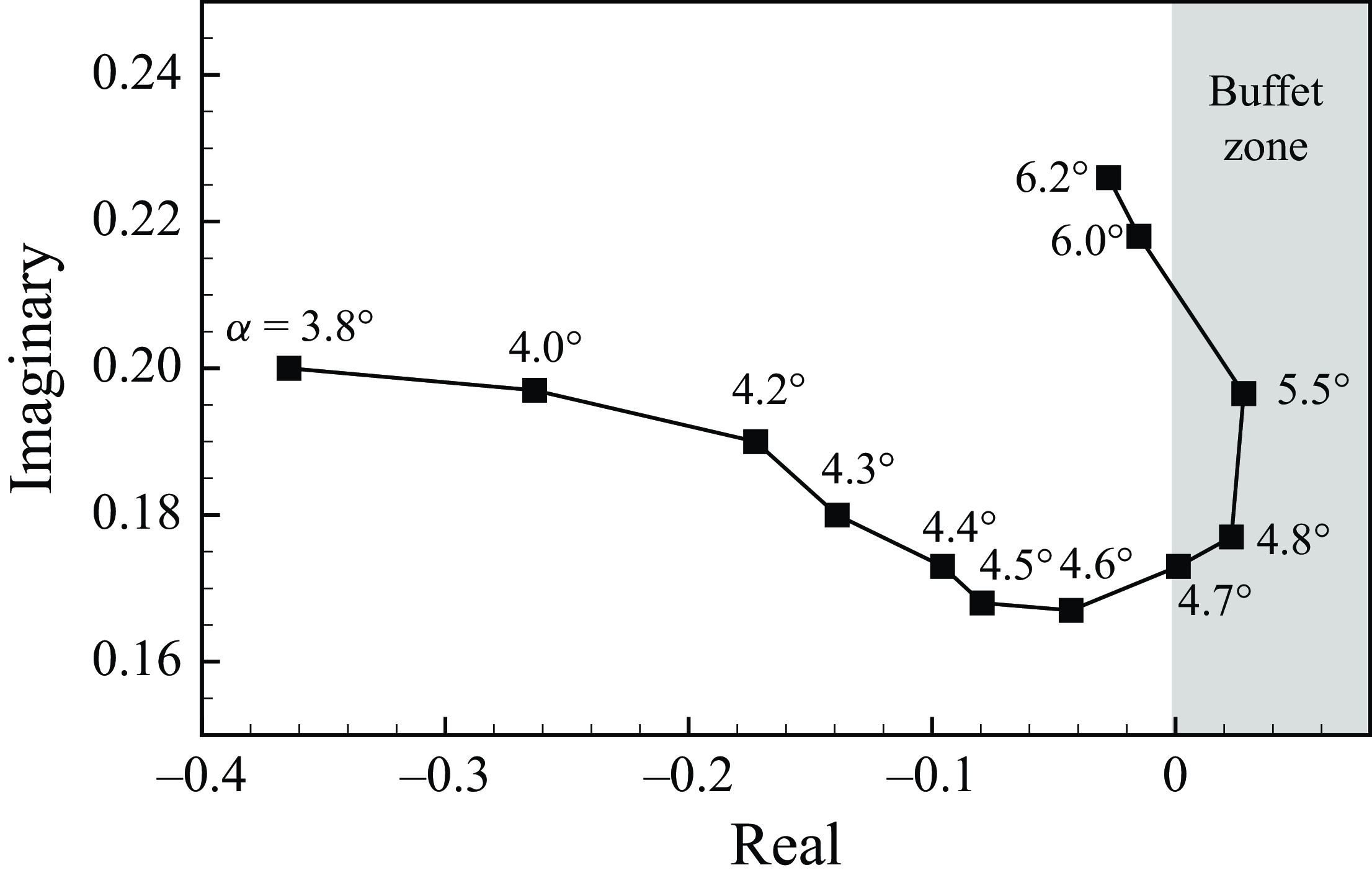
$\boldsymbol{A}$ , $\boldsymbol{B}$ , $\boldsymbol{C}$ are the coefficient matrices of the continuous-time form equations. $t$ represents the continuous time and $t_0$ is the continuous time delay between the input and output signal. Figure 9 shows the distribution of dominant eigenvalues of the matrix $\boldsymbol{A}$ at different angles of attack when ${\textit{Ma}}=0.7$ . The sign of the real part of the dominant eigenvalues represents the stability characteristics of the flow system. When it is positive, the flow system is unstable along with the appearance of the transonic shock buffet phenomenon, and vice versa. From the figure 9, it can be concluded that the model-predicted buffet-onset and offset angles of attack are approximately $4.8^\circ$ and $6^\circ$ , respectively, which are consistent with the CFD calculation results and the experimental results (Doerffer et al. Reference Doerffer, Hirsch, Dussauge, Babinsky and Barakos2010) shown in figure 3, validating that the modelling accuracy is satisfactory.

Figure 9.

Flow characteristic modes predicted by ARX model at different angles of attack when ${\textit{Ma}}=0.7$ .

Consequently, the aforementioned offline modelling method has been widely combined with model-based control design methods under time-invariant incoming flow conditions, achieving satisfactory control effects (Gao et al. Reference Gao, Zhang, Kou, Liu and Ye2017).

3.2. Inner-iterated time-variant reduced-order modelling method

However, for the adaptive control under time-variant conditions, the former established TI-ROM fails to provide accurate-enough aerodynamic prediction when the incoming flow conditions change, as it is difficult for designing an appropriate training signal or establishing a universal linear model for the system with time-variant intrinsic features, let alone correctly guide the flap’s actuation and achieve the control objectives.

To improve the high-precision prediction ability of the model under time-variant conditions and achieve the goal of overcoming the existing limitations of time-invariant models, this study develops a time-variant reduced-order modelling method based on the idea of local linearisation. With the ARX modelling architecture remaining unchanged, this method updates the model parameters online by rolling sampling the input/output data and applying the recursive least-square (RLS) method instead of the LS method introduced in § 3.1, simultaneously reducing the storage occupation. Figure 10 briefly introduces the sampling difference between the two modelling methods.

Figure 10.

Comparison of the two modelling frameworks.

The main idea of the RLS method is to transform the standard LS estimation equation (3.8) into the recursive form shown in the following expression (Pang & Cui Reference Pang and Cui2013):

(3.12) \begin{equation} \begin{aligned} \tilde {\boldsymbol{\theta }}(k)=\tilde {\boldsymbol{\theta }}(k-1)+\boldsymbol{\theta }_{\xi }(k), \end{aligned} \end{equation}

where $\tilde {\boldsymbol{\theta }}(k)$ represents the identified parameter matrix of the ROM at discrete time step $k$ and $\boldsymbol{\theta }_{\xi }(k)$ is the correction term between the parameter matrices of the adjacent two steps $(k-1)$ and $k$ .

Assume the identified parameter matrix at time step $k$ can be written as

(3.13) \begin{equation} \begin{aligned} \tilde {\boldsymbol{\theta }}(k)=\left[\boldsymbol{\varPhi }^{\mathrm{T}}(k)\boldsymbol{\varPhi }(k)\right]^{-1}\boldsymbol{\varPhi }^{\mathrm{T}}(k)\boldsymbol{Y}(k), \end{aligned} \end{equation}

where

(3.14) \begin{equation} \begin{aligned} \boldsymbol{\varPhi }(k)&=\begin{bmatrix}\boldsymbol{\varPhi }(k-1)\\\boldsymbol{x}^{\mathrm{T}}(k)\end{bmatrix}\in \mathbb{R}^{k\times (na+nb-d+1)},\\ \boldsymbol{Y}(k)&=\begin{bmatrix}\boldsymbol{Y}(k-1)\\y(k)\end{bmatrix}\in \mathbb{R}^{k\times 1}. \end{aligned} \end{equation}

Define

(3.15) \begin{equation} \begin{aligned} \boldsymbol{P}(k)&=[\boldsymbol{\varPhi }^{\mathrm{T}}(k)\boldsymbol{\varPhi }(k)]^{-1}\\ &=[\boldsymbol{\varPhi }^{\mathrm{T}}(k-1)\boldsymbol{\varPhi }(k-1)+\boldsymbol{x}(k)\boldsymbol{x}^{\mathrm{T}}(k)]^{-1}\\ &=[\boldsymbol{P}^{-1}(k-1)+\boldsymbol{x}(k)\boldsymbol{x}^{\mathrm{T}}(k)]^{-1}, \end{aligned} \end{equation}

then

(3.16) \begin{equation} \begin{aligned} \boldsymbol{P}^{-1}(k)=\boldsymbol{P}^{-1}(k-1)+\boldsymbol{x}(k)\boldsymbol{x}^{\mathrm{T}}(k). \end{aligned} \end{equation}

Substitute (3.16) into (3.13):

\begin{align*} \tilde {\boldsymbol{\theta }}(k)&=[\boldsymbol{\varPhi }^{\mathrm{T}}(k)\boldsymbol{\varPhi }(k)]^{-1}\boldsymbol{\varPhi }^{\mathrm{T}}(k)\boldsymbol{Y}(k) \nonumber \\&=\boldsymbol{P}(k)\boldsymbol{\varPhi }^{\mathrm{T}}(k)\boldsymbol{Y}(k) \nonumber\\&=\boldsymbol{P}(k)[\boldsymbol{\varPhi }^{\mathrm{T}}(k-1)\boldsymbol{Y}(k-1)+\boldsymbol{x}(k)y(k)]\nonumber\\&=\boldsymbol{P}(k)[\boldsymbol{P}^{-1}(k-1)\tilde {\boldsymbol{\theta }}(k-1)+\boldsymbol{x}(k)y(k)]\nonumber\\&=\boldsymbol{P}(k)\{[\boldsymbol{P}^{-1}(k)-\boldsymbol{x}(k)\boldsymbol{x}^{\mathrm{T}}(k)]\tilde {\boldsymbol{\theta }}(k-1)+\boldsymbol{x}(k)y(k)\}\nonumber\\ \end{align*}

(3.17) \begin{equation} \begin{aligned} &=\tilde {\boldsymbol{\theta }}(k-1)-\boldsymbol{P}(k)\boldsymbol{x}(k)\boldsymbol{x}^{\mathrm{T}}(k)\tilde {\boldsymbol{\theta }}(k-1)+\boldsymbol{P}(k)\boldsymbol{x}(k)y(k)\\&=\tilde {\boldsymbol{\theta }}(k-1)+\boldsymbol{P}(k)\boldsymbol{x}(k)[y(k)-\boldsymbol{x}^{\mathrm{T}}(k)\tilde {\boldsymbol{\theta }}(k-1)]. \end{aligned} \end{equation}

Further define

(3.18) \begin{equation} \begin{aligned} \boldsymbol{K}(k)=\boldsymbol{P}(k)\boldsymbol{x}(k). \end{aligned} \end{equation}

Based on the matrix inverse lemma

(3.19) \begin{equation} \begin{aligned} (\boldsymbol{A}+\boldsymbol{B}\boldsymbol{C})^{-1}=\boldsymbol{A}^{-1}-\boldsymbol{A}^{-1}\boldsymbol{B}(\boldsymbol{I}+\boldsymbol{C}\boldsymbol{A}^{-1}\boldsymbol{B})^{-1}\boldsymbol{C}\boldsymbol{A}^{-1}, \end{aligned} \end{equation}

where the matrices $\boldsymbol{A}$ , $(\boldsymbol{A}+\boldsymbol{B}\boldsymbol{C})$ and $(\boldsymbol{I}+\boldsymbol{C}\boldsymbol{A}^{-1}\boldsymbol{B})$ are required to be non-singular, we can let $\boldsymbol{A}=\boldsymbol{P}^{-1}(k-1)$ , $\boldsymbol{B}=\boldsymbol{x}(k)$ and $\boldsymbol{C}=\boldsymbol{x}^{\mathrm{T}}(k)$ and obtain

(3.20) \begin{equation} \begin{aligned} \boldsymbol{P}(k)=\boldsymbol{P}(k-1)-\boldsymbol{P}(k-1)\boldsymbol{x}(k)[1+\boldsymbol{x}^{\mathrm{T}}(k)\boldsymbol{P}(k-1)\boldsymbol{x}(k)]^{-1}\boldsymbol{x}^{\mathrm{T}}(k)\boldsymbol{P}(k-1). \end{aligned} \end{equation}

Take (3.20) back into (3.18):

(3.21) \begin{equation} \begin{aligned} \boldsymbol{K}(k)&=\boldsymbol{P}(k-1)\boldsymbol{x}(k)-\frac {\boldsymbol{P}(k-1)\boldsymbol{x}(k)\boldsymbol{x}^{\mathrm{T}}(k)\boldsymbol{P}(k-1)\boldsymbol{x}(k)}{1+\boldsymbol{x}^{\mathrm{T}}(k)\boldsymbol{P}(k-1)\boldsymbol{x}(k)}\\ &=\frac {\boldsymbol{P}(k-1)\boldsymbol{x}(k)[1+\boldsymbol{x}^{\mathrm{T}}(k)\boldsymbol{P}(k-1)\boldsymbol{x}(k)]-\boldsymbol{P}(k-1)\boldsymbol{x}(k)\boldsymbol{x}^{\mathrm{T}}(k)\boldsymbol{P}(k-1)\boldsymbol{x}(k)}{1+\boldsymbol{x}^{\mathrm{T}}(k)\boldsymbol{P}(k-1)\boldsymbol{x}(k)}\\ &=\frac {\boldsymbol{P}(k-1)\boldsymbol{x}(k)}{1+\boldsymbol{x}^{\mathrm{T}}(k)\boldsymbol{P}(k-1)\boldsymbol{x}(k)},\\ \boldsymbol{P}(k)&=[\boldsymbol{I}-\boldsymbol{K}(k)\boldsymbol{x}^{\mathrm{T}}(k)]\boldsymbol{P}(k-1). \end{aligned} \end{equation}

Until now, the RLS-based parameter identification process can be concluded as the following set of equations:

(3.22) \begin{equation} \left \{\begin{aligned} \tilde {\boldsymbol{\theta }}(k)&=\tilde {\boldsymbol{\theta }}(k-1)+\boldsymbol{K}(k)[y(k)-\boldsymbol{x}^{\mathrm{T}}(k)\tilde {\boldsymbol{\theta }}(k-1)],\\ \boldsymbol{K}(k)&=\frac {\boldsymbol{P}(k-1)\boldsymbol{x}(k)}{1+\boldsymbol{x}^{\mathrm{T}}(k)\boldsymbol{P}(k-1)\boldsymbol{x}(k)},\\ \boldsymbol{P}(k)&=[\boldsymbol{I}-\boldsymbol{K}(k)\boldsymbol{x}^{\mathrm{T}}(k)]\boldsymbol{P}(k-1). \end{aligned}\right . \end{equation}

To ensure that the ITV-ROM exhibits satisfactory accuracy at each time step, this study further introduces an inner iteration into the parameter update process. During the inner iteration, the model parameters are still updated by (3.22) with the input and output data unchanged until the following convergence criterion is met within each time step $k$ :

(3.23) \begin{equation} \begin{aligned} \Delta {\tilde {\boldsymbol{\theta }}}_k= \tilde {\boldsymbol{\theta }}_k(m)-\tilde {\boldsymbol{\theta }}_k(m-1) \leqslant \boldsymbol{\epsilon }, \end{aligned} \end{equation}

where $m \leqslant 100$ is the number of inner iterations for time step $k$ , and $\boldsymbol{\epsilon }$ is a sufficiently small vector with all positive real elements set to $10^{-6}$ in this paper.

This study activates the recursive formula through manually assigning the initial matrices as follows:

(3.24) \begin{equation} \left \{ \begin{aligned} \boldsymbol{P}(0)&=p\boldsymbol{I},\\ \tilde {\boldsymbol{\theta }}(0)&=\boldsymbol{\epsilon }, \end{aligned}\right . \end{equation}

where $p$ is a sufficiently large positive real number with a magnitude between $10^4$ and $10^{10}$ .

3.3. Comparison of the two modelling methods

This section further compares the identification ability of different modelling methods. The definition of the identification error is as follows:

(3.25) \begin{equation} \begin{aligned} \textit{Error} (\%) =\frac {\sum \limits _{k=1}^N\mid y(k)-\tilde {y}(k)\mid }{\sum \limits _{k=1}^N\mid y(k)\mid }, \end{aligned} \end{equation}

where $\tilde {y}(k)$ represents the response reversed by the ROM at time step $k$ , which is chosen as the lift coefficient response $C_l$ throughout the following study, and $N$ is the length of the input/output data. According to experience (Li, Zhang & Gao Reference Li, Zhang and Gao2018; Dou et al. Reference Dou, Gao and Zhang2024; Gao et al. Reference Gao, Yang, Ren and Zhang2025b ), the ARX model has a relatively high identification accuracy when $na=nb$ . Thus, this article considers only the case of $na=nb$ when identifying the model.

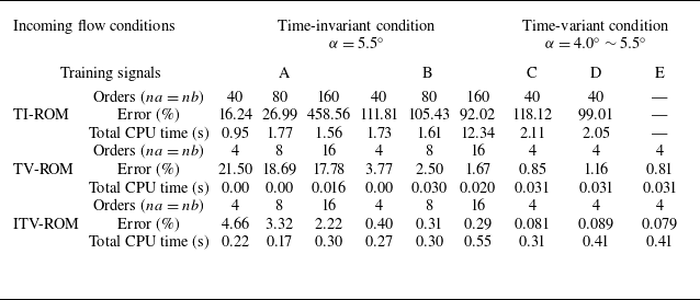
We designed five different training signals to test the identification ability and efficiency of TI-ROMs, TV-ROMs and ITV-ROMs under the previously introduced conditions, with the results depicted in table 1 and figure 11. Among them, signals A and B are used for the time-invariant buffet condition shown in figure 4, while signals C, D and E are meant for the time-variant condition shown in figure 5(a).

Table 1.

Comparison of modelling accuracy and computational efficiency across different ROM methods with different orders under different incoming flow conditions and training signals when ${\textit{Ma}}=0.70$ .

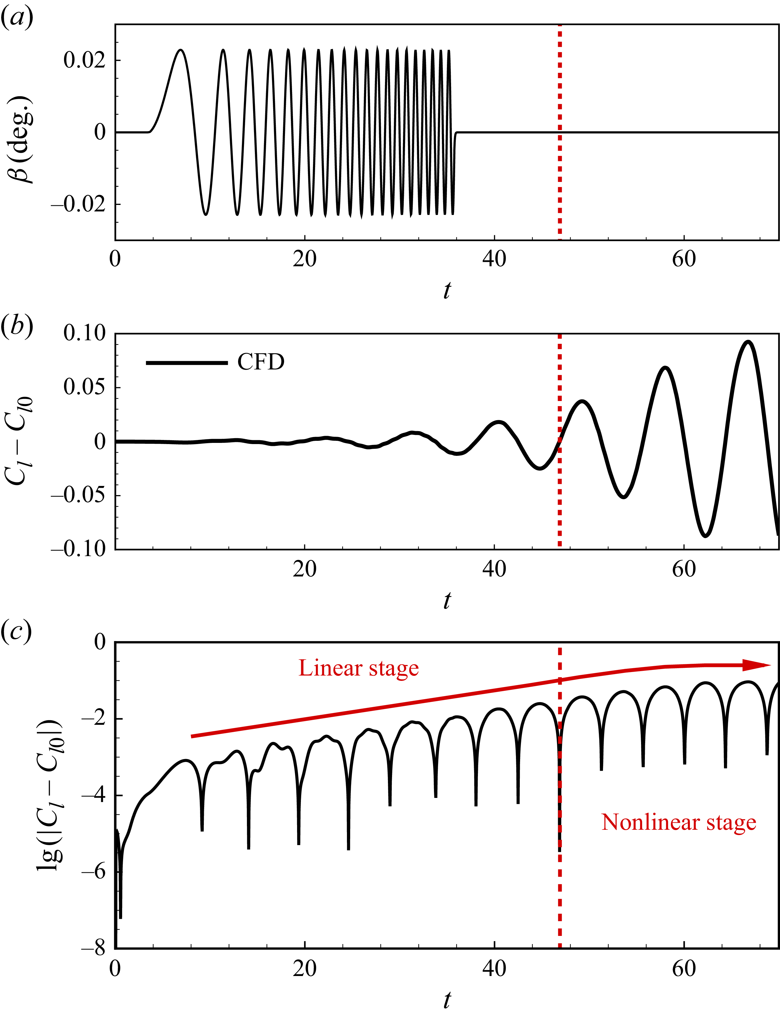
Both signals A and B act on the unstable steady base flow to ensure the stimulated unstable system remains at a linear developing stage as long as possible, thus enabling the TI-ROMs to work well. Signal A features constant amplitude and varying frequency within the range of $0.05 \leqslant St \leqslant 0.30$ , and its length is shorter than that of the linear developing stage of the flow system. Signal B is a signal formed by concatenating signal A with a zero signal, making the system freely develop to the nonlinear stage after the external excitation ends. The analysis of the output lift response stimulated by signal B is shown in figure 12.

Signal C is the superposition of two pulse signals with different amplitudes. The pulse signal with an amplitude of $0.2^{\circ }$ acts on the stable flow state of ${\textit{Ma}}=0.7, \alpha =4.0^{\circ }$ , while the pulse signal with an amplitude of $0.4^{\circ }$ acts on the buffet state. Signal D shares the same frequency with the transonic buffet flow over the NACA 0012 aerofoil at ${\textit{Ma}}=0.7, \alpha =5.5^{\circ }$ and its amplitude increases linearly from $0.2^{\circ }$ to $0.5^{\circ }$ . Signal E is a zero signal.

Table 1 systematically presents the identification error and time consumption of different modelling methods under different incoming flow conditions, training signals and delay orders. It can be seen that the TI-ROMs have good identification accuracy only when the proportion of non-zero signals is large enough and the flow system remains at a linear developing stage under time-invariant conditions. The TV-ROMs can stabilise the identification accuracy within $5\,\%$ when the signal length is long enough as it takes time for the parameters of TV-ROM to converge to the real system parameters. In comparison, the ITV-ROMs show the highest identification accuracy under various inflow conditions and training signals. At the same time, both TV-ROMs require a very small delay order, which is approximately 0.1 times that of the TI-ROMs, greatly reducing the storage usage and thus significantly improving the identification efficiency.

Figure 11 further exhibits the identification results, where the initial unstable steady lift coefficient $C_{l0}$ of time-invariant condition is 0.5529 and the stable lift coefficient of time-variant condition is $C_{l0}=0.5798$ . It can be concluded that the TV-ROMs have overcome the problem of linear models being unable to predict the response history of transition and nonlinear limit cycles. Meanwhile, the parameter update method with recursive characteristics also enables the TV-ROMs to perform response prediction work with zero input.

Figure 11.

Comparison of the identified responses under different incoming flow conditions and training signals.

Figure 12.

Analysis of the response developing process from the unstable steady base flow with the excitation of training signal B at ${\textit{Ma}}=0.7, \alpha =5.5^{\circ }$ .

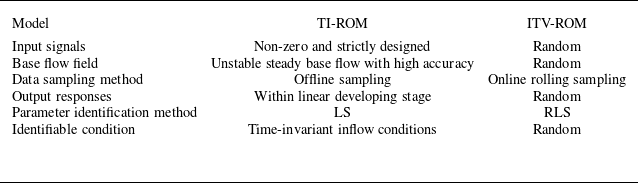
Table 2 concludes the improvement of the ITV-ROMs compared with the TI-ROMs. As it illustrates, the ITV-ROMs improve the global predictive ability of the linear model for nonlinear flow-system response through a rolling sampling strategy and RLS-based parameter update strategy. They also significantly reduce the amount of storage occupied in the model identification process, improve identification efficiency, and provide new possibilities for feedback control design work combined with model-based adaptive control methods. As four-order ITV-ROM is accurate enough in response prediction, so this study fixes the orders of ITV-ROM as $na=nb=4$ .

4.1. Methodology of MVC

Minimum variance control is designed with the goal of minimising output variance. Due to the delay normally existing in dynamics systems, assuming a delay of $d$ , the current control may make an effect on the system output after $d$ sampling time steps. Therefore, in order to minimise the output variance, it is necessary to make predictions on the output in advance, and then design the required control law based on the predicted values obtained. By continuously predicting and conducting control instructions, it is possible to ensure that the steady-state output variance is minimised. It can be seen that the key to achieving MVC lies in the accuracy of output prediction.

Table 2.

Improvement of the ITV-ROMs compared with the TI-ROMs.

The specific steps of MVC are as follows. To begin with, the difference equations shown in (3.1) need to be transformed into a discrete-time form using the z-transform, demonstrated as follows with the assumption of $\xi (k)=0$ :

(4.1) \begin{equation} A(z^{-1})y(k)=z^{-d}B(z^{-1})u(k). \end{equation}

The parameters of the coefficient matrices can be obtained through the RLS method introduced in § 3.2, the representations of which are as follows:

(4.2) \begin{equation} \left \{ \!\!\begin{array}{l} A(z^{-1})=1-A_1z^{-1}-A_2z^{-2}-{\cdots} -A_{na}z^{-na},\\ B(z^{-1})=B_d+B_{d+1}z^{-1}+B_{d+2}z^{-2}+{\cdots} +B_{nb}z^{-nb+d},B_d\neq 0.\\ \end{array} \right . \end{equation}

Calculate the future output $\tilde {y}(k+d|k)$ at time step $(k+d)$ predicted by the ITV-ROM established at time step $k$ as the preparation of the control law design process. The control target applied in this section is to minimise the variance between the predicted output and the expected output, with the performance metric $J$ shown as follows:

(4.3) \begin{equation} J=\mathbf{E}\left\{[\tilde {y}(k+d)-y_r(k+d)]^2\right\}\!. \end{equation}

Here, $y_r(k+d)$ is the target output defined by the researcher based on the system characteristics, which can be the mean system response or the unstable steady response solution.

According to the optimal control requirements, if targeting at minimising the performance metric $J$ , the MVC law can be obtained as follows:

(4.4) \begin{equation} F(z^{-1})u(k)=y_r(k+d)-G(z^{-1})y(k), \end{equation}

where

(4.5) \begin{equation} \left \{\!\!\begin{array}{l} 1=A(z^{-1})E(z^{-1})+z^{-d}G(z^{-1}),\\ F(z^{-1})=B(z^{-1})E(z^{-1}), \end{array}\right . \end{equation}

and

(4.6) \begin{align} \left \{\!\!\begin{array}{l} E(z^{-1})=1+e_{1}z^{-1}+e_{2}z^{-2}+{\cdots} +e_{ne}z^{-ne},(ne=d-1)\\ G(z^{-1})=g_0+g_1z^{-1}+g_2z^{-2}+{\cdots} +g_{ng}z^{-ng},(ng=na-1)\\ F(z^{-1})=f_{0}+f_{1}z^{-1}+f_{2}z^{-2}+{\cdots} +f_{nf}z^{-nf},(nf=nb+d-1). \end{array}\right . \end{align}

Similar to $A(z^{-1})$ and $B(z^{-1})$ , $E(z^{-1})$ , $F(z^{-1})$ , and $G(z^{-1})$ are also polynomials obtained through $z$ -transform, where $e_i$ , $f_i$ , $g_i$ are the coefficients awaiting to be solved through (4.5). $ne$ , $ng$ , $nf$ are the orders of these polynomials, respectively.

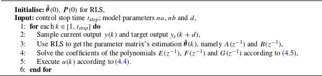
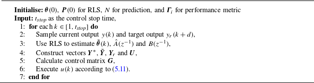
The whole MVC algorithm can be concluded as Algorithm1.

Algorithm 1

algorithm of MVC

Notably, take (4.1) into (4.4) and then the expression of the input and the output can be turned into

(4.7) \begin{equation} \left \{ \begin{array}{l} u(k)=\dfrac {\dfrac {1}{F}}{1+\dfrac {z^{-d}B}{A}\dfrac {G}{F}} y_r(k+d)+\dfrac {-\dfrac {1}{A}\dfrac {G}{F}}{1+\dfrac {z^{-d}B}{A}\dfrac {G}{F}}\xi (k)=\dfrac {Ay_r(k+d)-G\xi (k)}{B},\\[15pt] y(k)=\dfrac {z^{-d}B}Au(k)+\dfrac {1}{A}\xi (k)=y_r(k)+E\xi (k), \end{array} \right . \end{equation}

where $A$ , $B$ , $E$ , $F$ and $G$ are the abbreviations of $A(z^{-1})$ , $B(z^{-1})$ , $E(z^{-1})$ , $F(z^{-1})$ and $G(z^{-1})$ . It can be concluded that the essence of MVC is to use the pole of the controller (the zero of $F(z^{-1})$ ) to cancel the zero of the controlled object (the zero of $B(z^{-1})$ ). According to (4.7), when $B(z^{-1})$ is unstable, the control input $u(k)$ will increase exponentially and reach the saturation, eventually resulting in the instability of the flow-control coupled system (Sipp & Schmid Reference Sipp and Schmid2016).

Unfortunately, the controlled object of this study shows a great potential in having unstable zeros of $B(z^{-1})$ as the transonic buffet flow system itself is a highly nonlinear system with strong instability. Figure 13 shows the trajectories of the zeros of $B(z^{-1})$ obtained through the ITV-ROM under the condition shown in figure 5. It is obvious that when the shock wave buffet phenomenon begins to occur, the stable zeros of $B(z^{-1})$ quickly change to unstable ones (changing from inside the black stable boundary to outside). Therefore, it is necessary to take certain actions on the choice of the expected output $y_r(k+d)$ to overcome the influence of the existing unstable zeros of $B(z^{-1})$ when applying ITV-ROM-based MVC method for closed-loop control design.

Figure 13.

The trajectories of the zeros of $B(z^{-1})$ under the time-variant condition when ${\textit{Ma}}=0.70, \alpha =4.0^{\circ } \sim 5.5^{\circ }$ .

4.2. MVC for transonic buffet

In the numerical simulation environment, it can be approximately assumed that the transonic buffet flow response has no significant delay on the control input, namely $d=0$ . Take the lift coefficient response $C_l$ as the model output and also the feedback data. Therefore, the performance metric of MVC can be expressed as

(4.8) \begin{equation} J=E\left\{[C_l(k)-C_{lr}(k)]^2\right\}\!. \end{equation}

And the minimum variance self-tuning control law shown in (4.7) can be further simplified as follows:

(4.9) \begin{equation} \beta (k)=\dfrac {A(k)C_{lr}(k)}{B(k)}. \end{equation}

In this equation, $\beta (k)$ represents the deflection of the trailing-edge flap, $A(k)$ and $B(k)$ are the identified parameter matrices and $C_{lr}(k)$ signifies the target lift coefficient output, all specified at time $k$ .

4.2.1. Influence of different target outputs

The ideal effect of transonic buffet control is to make the self-excited oscillation shock wave stationary, and the unstable flow eventually approaches a steady state without changing the incoming flow conditions and the shape of the aerofoil. This steady state strictly satisfies the boundary conditions and control equations in mathematics, that is, the unstable steady solution of the flow system. In previous research, such as the work of Ren et al. (Reference Ren, Gao, Xiong and Zhang2024), the unstable steady solution was used as a reference for optimal DRL control, thereby achieving complete suppression of buffet loads. Therefore, the lift coefficient corresponding to the unstable steady solution is first employed as the target output of the control system in this paper.

This article first conducts research on the control of transonic buffet over a NACA 0012 aerofoil in the state of ${\textit{Ma}}=0.7$ and $\alpha =5.5^\circ$ , where the buffet phenomenon is relatively apparent. Gao et al. (Reference Gao, Zhang, Kou, Liu and Ye2017) once carried out transonic buffet control research under this state, achieving complete suppression of the fluctuating loads through the linear quadratic (LQ) method. The unstable steady lift coefficient after control is $C_{l0}=0.5529$ , and the non-dimensional pressure distribution in this state is presented in figure 14.

Figure 14.

The pressure distribution of the unstable steady solution when ${\textit{Ma}}=0.70$ , $\alpha =5.5^\circ$ .

Considering the influence of the unstable zeros of $B(z^{-1})$ , this paper chooses to linearly soften the target output in order to avoid situations where the initial deflection angle of the trailing-edge flap could cause significant disturbances to the sensitive flow system or exceed the maximum deformation limits allowed by the dynamic grid method, both of which may lead to simulation failure (see Appendix B for details). Specifically, it is to introduce a softening coefficient $\gamma$ to balance the weight of unstable steady solution and the last step output. The target output is constructed by the linear superposition of these two terms as follows:

(4.10) \begin{equation} C_{lr}(k)=(1-\gamma )C_{l0}+\gamma C_l(k-1). \end{equation}

The control effects under different softening coefficients are compared in figure 15. It can be seen that after increasing the softening coefficient, the impact caused by instantaneous deformation is reduced, and the deflection angle of the flap is within the acceptable range of the dynamic grid method. The larger the softening coefficient, the smaller the difference between the target output and the current output, and the smaller the impact of the flap actuation on the flow system when starting control. With the two typical softening coefficients depicted in figure 15, complete suppression of buffet loads can be achieved. Ultimately, the flap angle stabilises at $0^{\circ }$ , the lift coefficient $C_l$ settles at the unstable steady solution of 0.5529, and the torque coefficient $C_m$ also tends to stabilise. From the analysis, it is evident that using the unstable steady solution as the target output can effectively suppress transonic buffet loads within quite a short adjustment period. However, there are still certain challenges in utilising unstable steady solutions as target outputs. Firstly, the potential significant discrepancy between the current output and the unstable steady solution may lead to an inescapable huge impact at the very beginning of control. Although this problem can be mitigated by limiting the controller amplitude and introducing a softening coefficient, there is still a risk of excessive adjustment time. Secondly, unstable steady solutions are not a universal target output, and, in many cases, the performance of the controlled system remains unknown, which poses significant challenges in obtaining unstable steady solutions in advance. Especially in adaptive control scenarios, where the system undergoes real-time changes under varying inflow conditions, obtaining the unstable steady solution beforehand for such continuously evolving flows is unrealistic. Therefore, it is necessary to define a more universal target output based on the response characteristics of transonic buffet.

Figure 15.

Comparison of control effects under different softening coefficients when ${\textit{Ma}}=0.70$ , $\alpha =5.5^\circ$ .

Considering that the lift coefficient response of transonic buffet exhibits an approximate harmonic response, this paper tends to employ the mean lift coefficient response over $q$ time steps before current time step $k$ as the target output, as follows:

(4.11) \begin{equation} C_{lr}(k)=\frac {C_l(k-1)+C_l(k-2)+{\cdots} +C_l(k-q)}q. \end{equation}

Figure 16.

Buffet control effect under time-averaged target output with different $q$ when ${\textit{Ma}}=0.70$ , $\alpha =5.5^\circ$ .

This time-averaged target output changes in real time, thus overcoming the disadvantages of unstable steady solutions and facilitating the adaptive control system to efficiently achieve control objectives.

Figure 16 shows the control results under different values of forward time step $q$ , where $q=226$ corresponds to the number of simulation steps within a single period of transonic buffet at ${\textit{Ma}}=0.7$ and $\alpha =5.5^\circ$ . It is evident that complete suppression of control objectives is achieved for varying values of $q$ . The inevitable impact of control increases with the increase of $q$ as the difference between current output and the target output increases. Nevertheless, this impact remains within the acceptable range for the dynamic grid method. In addition, the lift coefficient and flap deflection angle both tend to non-oscillatory stable states. However, these steady states differ from those observed in the unstable steady solution depicted in figure 15. To be more specific, when $q=10$ and $q=20$ , there are stable positive flap deflection angles of $5.1^\circ$ and $4.1^\circ$ , respectively; when $q=226$ , the flap deflection angle converges to approximately $-1.5^\circ$ which means that the flap ultimately deflects upward under this situation. It means that the stable deflection of the control surface adjusts the equivalent angle of attack of the aerofoil to either below the buffet-onset boundary or above the buffet-offset boundary, thereby suppressing the unsteady aerodynamic loads caused by flow separation.

This control mechanism is similar to the TED methods. However, changing the equivalent angle of attack through relevant control devices is usually undesirable during the transonic cruising state of an aircraft, as it can result in lowered mean $C_l$ (as shown in figure 16 b) and compromised aerodynamic efficiency. To avoid this, the final flap deflection angle should be constrained through appropriate design of the control performance metric.

4.2.2. Validation of MVC’s effectiveness

This section further verifies the control effect of MVC at ${\textit{Ma}}=0.75$ and $\alpha =3.5^\circ$ , which employs the time-averaged lift coefficient calculated by (4.11) as the target output, with $q=20$ . The control results of MVC at this state are shown in figure 17.

Figure 17.

Control effect of MVC at ${\textit{Ma}}=0.75$ and $\alpha =3.5^\circ$ .

As the figure illustrates, when control starts, the fluctuation characteristics of the lift coefficient rapidly weaken and its value ultimately converges to a nearly stable state around $0.34$ , which is close to the unstable steady solution $C_{l0}=0.357$ obtained in the work of Gao et al. (Reference Gao, Zhang and Ye2016). The performance metric $J$ also rapidly decays and approaches  $0$ . From the perspective of the responses of lift coefficient and performance metric, it can be concluded that MVC eventually achieves satisfactory suppression of buffet loads. However, despite the convergence of the lift coefficient response to a stable value, the flap continues to actuate with an amplitude of approximately $3^\circ$ , rather than converging to $0^\circ$ as shown in figure 16. Additionally, the shock wave and torque coefficient also exhibit continuous oscillation (with the torque integration point at $25\,\%$ chord length), indicating that while the flap oscillation controls the lift load, the shock waves in the flow field remain unstable.

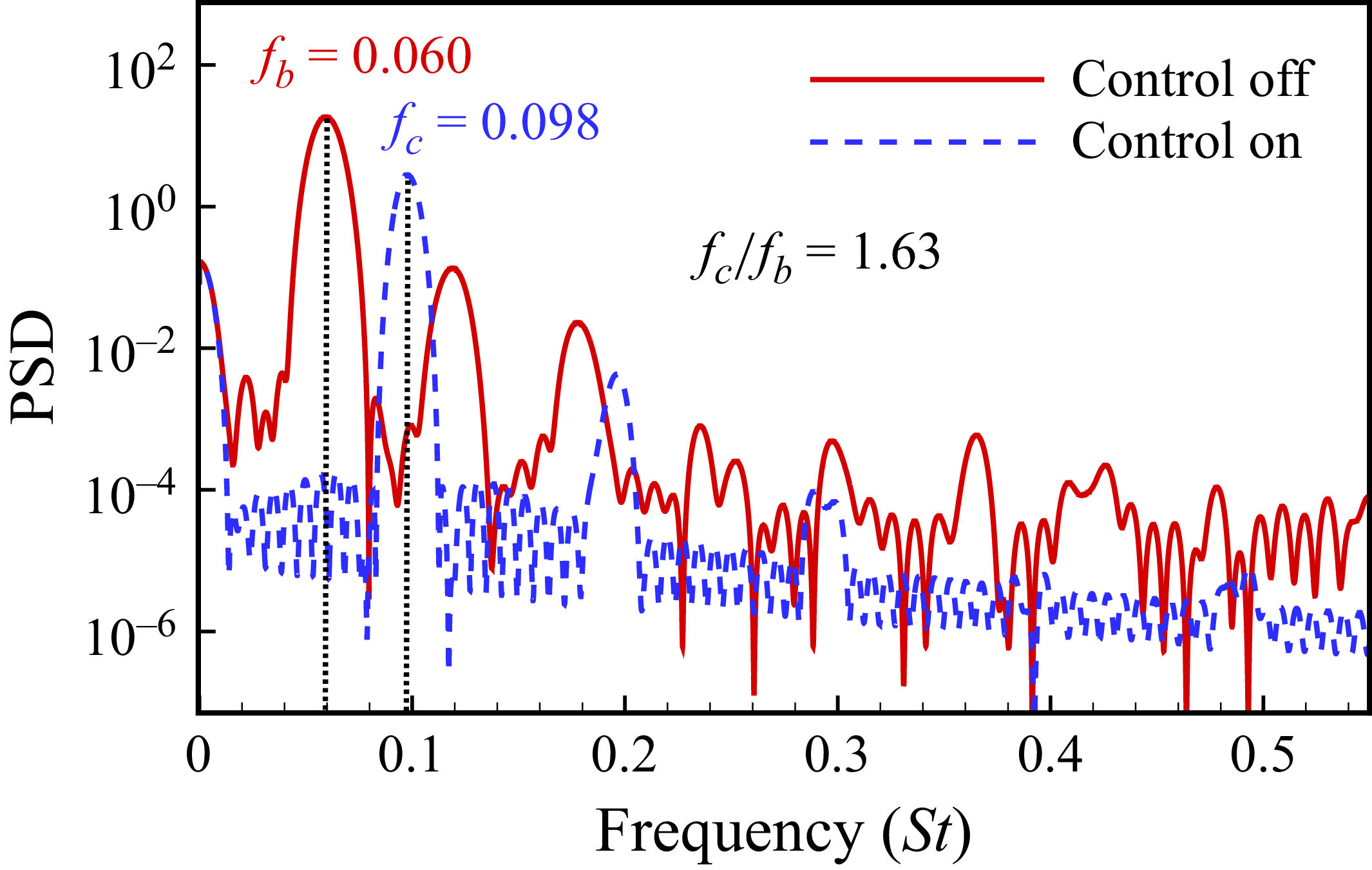
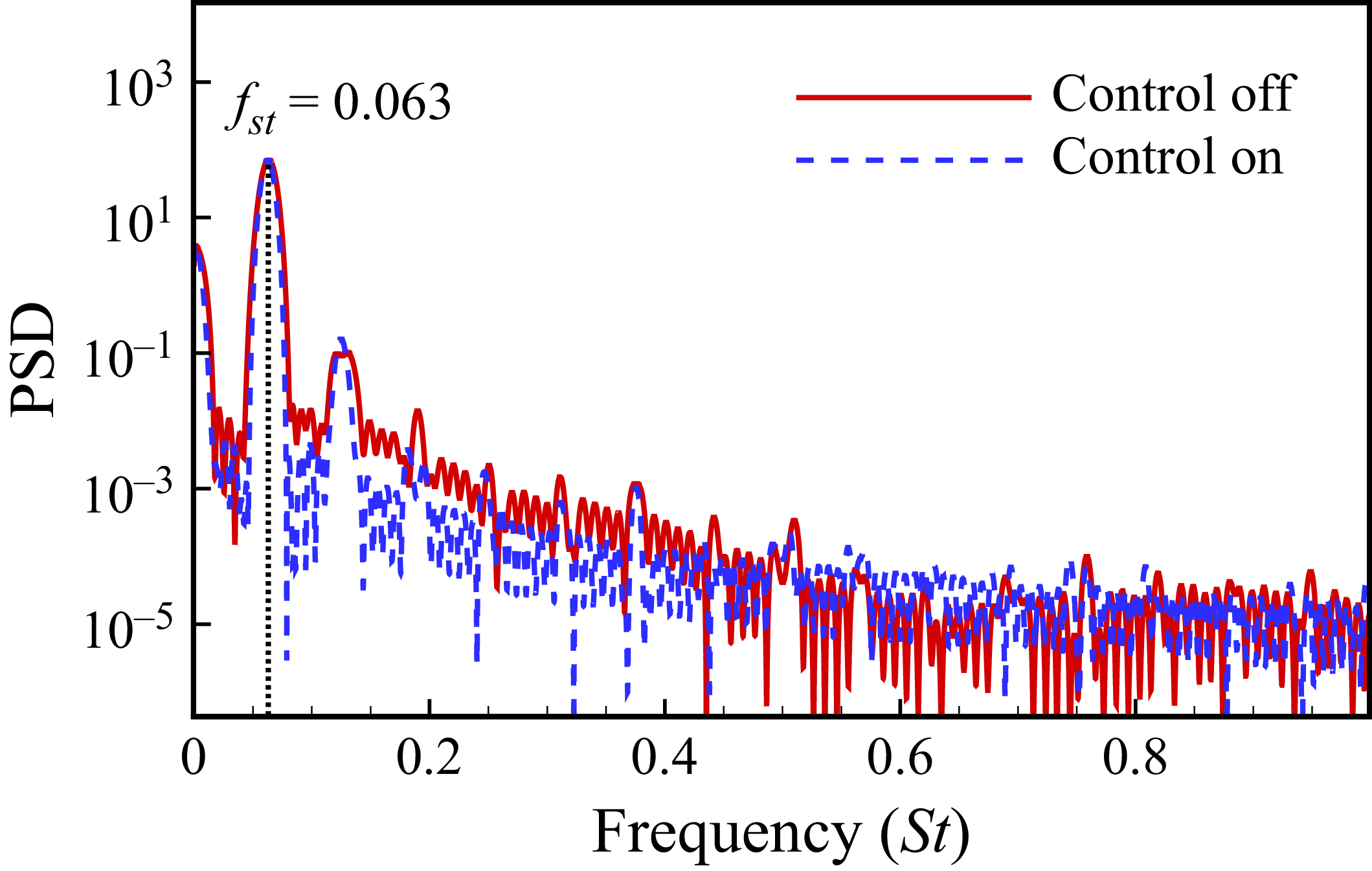
Next, the mechanism behind this interesting phenomenon is further analysed. Figure 18 shows the power spectrum analysis results of the torque coefficient response before and after control. It can be seen that the dimensionless frequencies of the response before and after control are separately $f_b=0.060$ and $f_c=0.098$ (equal to the actuating frequency of flap). The latter frequency is 1.63 times the former one ( $f_c/f_b=1.63$ ), which is consistent with the optimal open-loop control frequency ratio obtained in the work of Gao et al. (Reference Gao, Zhang, Kou, Liu and Ye2017) through extensive simulations.

Figure 18.

Power spectrum analysis results of torque coefficient response with and without MVC at ${\textit{Ma}}=0.75$ and $\alpha =3.5^\circ$ . PSD-Power Spectral Density.

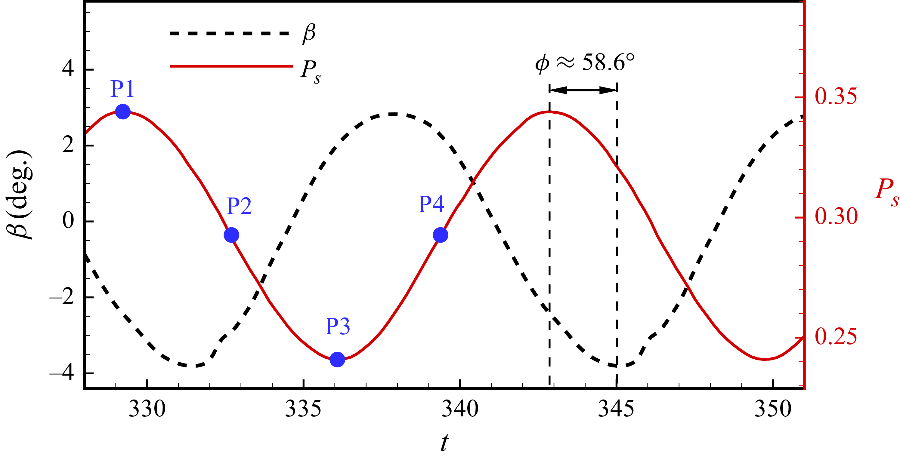
Figure 19 further demonstrates the relationship between the flap deflection angle and the position of the shock wave after stabilising the control response. According to the definition, the downward deflection of the control surface is positive. The figure reveals that the deflection of the control surface and the position of the shock wave both exhibit approximately harmonic response characteristics, with nearly identical response periods. Based on these response characteristics, this paper further calculates the phase difference between the shock wave oscillation response and the flap deflection, revealing a lag phase angle $\phi$ of approximately $58.6^\circ$ . Comparing this with the delay of the lift coefficient response on flap deflection, estimated to be approximately $60^\circ$ using the phase delay calculation method proposed by Gao et al. (Reference Gao, Zhang, Kou, Liu and Ye2017) for subcritical states, we find that the two delay phase angles are nearly identical. In essence, given the minimal phase delay in the aerodynamic response (the aerodynamic response and shock wave oscillation response are almost synchronous) to the flap deflection, the designed closed-loop control law functions effectively as an inverse control mechanism for both shock wave oscillation and aerodynamic responses.

Figure 20 shows a comparison of pressure coefficients, flow field cloud maps and flap deflections at several typical states labelled in figure 19. When the shock wave reaches its maximum position ${P}_{s}=0.344$ , the area enclosed by the leading edge of the aerofoil and the shock wave position is relatively large. At this time, if taking the phase delay into consideration, the flap deflects precisely at the maximum upward position. The upward deflection of the control surface is equivalent to reducing the effective angle of attack of the aerofoil, and the lift coefficient caused by the flap’s motion is negative, as shown in figure 20(a). Therefore, although the shock wave in this state is at the rear, the upward flap deflection guided by feedback control partially offsets the lift coefficient, resulting in a total lift coefficient of $0.34$ . When the shock wave reaches the forward position at ${P}_{s}=0.241$ , although the area enclosed by the leading edge of the aerofoil to the shock wave position is small, the control surface deflects precisely to its maximum downward position, which is equivalent to increasing the effective angle of attack of the aerofoil, thus increasing the lift coefficient and compensating for the loss of lift coefficient caused by the shock wave’s forward movement. So the total lift coefficient remains equal to 0.34. Similarly, in other states, although the position of the shock wave changes and the lift coefficient generated by the shock wave is slightly different, feedback control can always guide the corresponding flap deflection based on the inverse control mechanism, adjust the lift coefficient, and maintain the total lift coefficient at 0.34.

Figure 19.

The relationship between shock wave oscillation and flap deflection under feedback control when ${\textit{Ma}}=0.75$ , $\alpha =3.5^\circ$ .

Figure 20.

Comparison of pressure coefficients, flow field cloud maps and flap deflections under typical conditions after MVC at ${\textit{Ma}}=0.75$ and $\alpha =3.5^\circ$ .

From the analysis, it can be seen that the closed-loop flap control strategy guided by MVC based on the ITV-ROM achieves a similar effect to the open-loop control in the work of Gao et al. (Reference Gao, Zhang, Kou, Liu and Ye2017), which further demonstrates that the actuator frequency is a crucial parameter in open-loop control. Although this control law can effectively suppress the fluctuation of the lift coefficient, the flap deflection angle still changes harmonically, and the flow field does not reach a steady state ultimately. This phenomenon can be attributed to the lack of constraints on the control input in the construction of the performance metric shown in (4.3). Therefore, when the lift coefficient approaches the target value, the flow field may not necessarily reach a steady state. If constraints are imposed on both the lift coefficient and the control input (flap deflection angle), the flow field will also reach a steady state when both the lift coefficient and flap angle approach the target value.

5.1. Methodology of GPC

Consider the discrete-time system described in (4.1) and transform it into (5.1) to describe the relationship between control input increment and response output:

(5.1) \begin{equation} \hat {A}(z^{-1})y(k)=z^{-d}B(z^{-1})\Delta u(k), \end{equation}

where

(5.2) \begin{align} \left \{\begin{aligned} \hat {A}(z^{-1})&=A(z^{-1})(1-z^{-1})=1+a_{1,1}z^{-1}+{\cdots} +a_{1,na+1}z^{-(na+1)},\\ B(z^{-1})&=b_{1,0}+b_{1,1}z^{-1}+{\cdots} +b_{1,nb}z^{-nb}, \end{aligned}\right . \end{align}

and $a_{1,0}=1$ , $a_{1,na+1}=A_{na}$ ; $a_{1,i}=-A_i+A_{i-1}$ , $1 \leqslant i \leqslant na$ ; $b_{1,j} = B_{d+j}$ , $0 \leqslant i \leqslant nb$ .

The minimum variance output prediction model of the system at the future time $(k+N)$ can be written as:

(5.3) \begin{equation} \boldsymbol{Y}^*=\tilde {\boldsymbol{Y}}+\boldsymbol{G}\Delta \boldsymbol{U}, \end{equation}

where

(5.4) \begin{align} \left \{\begin{aligned} &\boldsymbol{Y}^*=[y^*(k+d\mid k),y^*(k+d+1\mid k),{\cdots} ,y^*(k+N\mid k)]^{\mathrm{T}},\\ &\tilde {\boldsymbol{Y}}=[\tilde {y}(k+d),\tilde {y}(k+d+1),{\cdots} ,\tilde {y}(k+N)]^{\mathrm{T}},\\ &\boldsymbol{U}=[u(k),u(k+1),{\cdots} ,u(k+N-d)]^{\mathrm{T}},\\ &\Delta u(k+i)=u(k+i)-u(k+i-1),i=0,1,{\cdots} ,N-d,\\ &\Delta \boldsymbol{U}=[\Delta u(k),\Delta u(k+1),{\cdots} ,\Delta u(k+N-d)]^{\mathrm{T}},\\ &\boldsymbol{G}=\begin{bmatrix}b_{1,0}&0&{\cdots} &0\\b_{2,0}&b_{1,0}&{\cdots} &0\\\vdots &\vdots &\ddots &\vdots \\b_{N-d+1,0}&b_{N-d,0}&{\cdots} &b_{1,0}\end{bmatrix}_{(N-d+1)\times (N-d+1)}. \end{aligned}\right . \end{align}

The predicted output $\tilde {y}(k+j)$ of step $(k+j)$ can be expressed as

(5.5) \begin{equation} \begin{aligned}\tilde {y}(k+j)=\sum _{i=1}^{na}a_{1,i}\tilde {y}(k+j-i)+\sum _{i=0}^{nb}b_{1,i}\Delta u(k+j-d-i|k), j=1,2,{\cdots} ,N,\end{aligned} \end{equation}

where

(5.6) \begin{align} \left \{\begin{aligned} &\tilde {y}(k+i)=y(k+i),i\leqslant 0,\\ &u(k+i | k)=\begin{cases}0,i\gt 0\\u(k+i),i\leqslant 0.\end{cases} \end{aligned}\right . \end{align}

The elements in the control matrix $\boldsymbol{G}$ are recursively obtained from the following equation:

(5.7) \begin{equation} b_{j,0}=b_{1,j-1}-\sum _{i=1}^{j_1}a_{1,i}b_{j-i,0},\quad j=2,3,{\cdots} ,N-d+1, \end{equation}

in which $j_1=\min \{j-1,na\}$ . When $j-1\gt nb$ , $b_{1,j-1}$ equals to $0$ .

After obtaining the predicted output at time $N$ , the target reference output sequence $\boldsymbol{Y}_{\! r}$ can be constructed:

(5.8) \begin{equation} \boldsymbol{Y}_{\! r}=[y_r(k+d),y_r(k+d+1),{\cdots} ,y_r(k+N)]^{\mathrm{T}}. \end{equation}

In control law design, the variance of the actual output over the target output and the controller characteristic weighting index are used as the control objectives, and the performance metric of GPC is defined as follows, where $\boldsymbol{\varGamma }_{\! i}=\varGamma _i\boldsymbol{I}$ ( $1\leqslant i\leqslant (N-d+1)$ ) represent the weight matrices:

(5.9) \begin{equation} \begin{aligned}J&=J_1+J_2+J_3\\&=E\{(\boldsymbol{Y}-\boldsymbol{Y}_{\! r})^{\mathrm{T}}(\boldsymbol{Y}-\boldsymbol{Y}_{\! r})+(\boldsymbol{U}+\Delta \boldsymbol{U})^{\mathrm{T}}\boldsymbol{\varGamma }_{\! 1}(\boldsymbol{U}+\Delta \boldsymbol{U})+\Delta \boldsymbol{U}^{\mathrm{T}}\boldsymbol{\varGamma }_{\! 2}\Delta \boldsymbol{U}\}.\end{aligned} \end{equation}

The performance metric can be further decomposed into three components, which are $J_1=E\{(\boldsymbol{Y}-\boldsymbol{Y}_{\! r})^{\mathrm{T}}(\boldsymbol{Y}-\boldsymbol{Y}_{\! r})\}$ representing the constraint that ensures the outputs approach those of the target, $J_2=E\{(\boldsymbol{U}+\Delta \boldsymbol{U})^{\mathrm{T}}\boldsymbol{\varGamma }_{\! 1}(\boldsymbol{U}+\Delta \boldsymbol{U})\}$ aiming to minimise the amplitude of inputs and $J_3=E\{\Delta \boldsymbol{U}^{\mathrm{T}}\boldsymbol{\varGamma }_{\! 2}\Delta \boldsymbol{U}\}$ limiting the changes in inputs between two consecutive time steps to prevent huge impacts to the flow system. By minimising the performance metric as the optimisation direction, the expression for the control increment vector can be obtained as follows:

(5.10) \begin{equation} \Delta \boldsymbol{U}=(\boldsymbol{G}^{\mathrm{T}}\boldsymbol{G}+\boldsymbol{\varGamma}_{\! 1}+\boldsymbol{\varGamma }_{\! 2})^{-1}[\boldsymbol{G}^{\mathrm{T}}(\boldsymbol{Y}_{\! r}-\tilde {\boldsymbol{Y}})-\boldsymbol{\varGamma }_{\! 1} \boldsymbol{U}]. \end{equation}

Therefore, the control input at time step $k$ can be written as follows:

(5.11) \begin{equation} u(k)=u(k-1)+\Delta u(k), \end{equation}

The whole GPC algorithm can be concluded as Algorithm2.

Algorithm 2

algorithm of GPC

Compared with MVC, there are two typical improvements in GPC. The first is that the performance metric of GPC additionally introduces two weighted terms, $J_2$ and $J_3$ , considering the input amplitude and change amount of the controller separately. This introduction can effectively overcome the disadvantage of MVC which lacks constraints on input. The second is that the control objective in GPC is not a fixed global optimisation objective, but a finite-time domain optimisation control employing a rolling optimisation strategy. Control is conducted repeatedly online, rather than offline in a single instance. At each sampling time, the control performance metric incorporates the future finite-time domain which advances synchronously with the sampling time. This limited time domain optimisation objective may only yield global suboptimal solutions, but the controller can effectively track and adapt to the system’s local dynamic characteristics in real time through repeated online model prediction and control. Therefore, the control system maintains effective optimality and achieves the goal of adaptive control, particularly in scenarios with time-variant incoming flow conditions.

5.2. GPC for transonic buffet

This section adopts the same assumptions as § 4.2. According to the framework of GPC, it is necessary to determine the target reference output sequence. Considering the difficulty in obtaining the unstable steady solution of the transonic buffet system, the average lift coefficient response over a period of time is used as the target reference output, as follows:

(5.12) \begin{equation} \left \{ \begin{array}{l} \boldsymbol{Y}_{\! r}=[y_r(k),y_r(k+1),{\cdots} ,y_r(k+N)]^{\mathrm{T}},\\[6pt] y_r(k+i)=y_r(k),i=0,{\cdots} ,N,\\[6pt] y_r(k)=\dfrac {C_l(k-1)+C_l(k-2)+{\cdots} +C_l(k-q)}q. \end{array} \right . \end{equation}

The deflection law of the trailing-edge flap designed by GPC can be formulated as follows:

(5.13) \begin{equation} \begin{aligned} \beta (k)&=\beta (k-1)+\Delta \beta (k)\\&=\beta (k-1)+[1,0,{\cdots} ,0]\Delta \boldsymbol{U}, \end{aligned} \end{equation}

where $\Delta \boldsymbol{U}$ is calculated by (5.10).

5.2.1. Influence of controller parameters

From the design framework of GPC, the controller consists of three sets of variable parameters, namely the width $N$ of recursive prediction, the number of forward time steps $q$ for constructing the target output, and the weighted coefficients $\varGamma _1$ and $\varGamma _2$ in the performance metric. The influence of these parameters on the control effect is studied in this section at ${\textit{Ma}}=0.70$ and $\alpha =5.5^\circ$ .

We first investigate the influence of the two weighted coefficients and other parameters are set as $N=4$ and $q=20$ . As (5.9) shows, $\varGamma _1$ represents the weight of the actuation amplitude of flap in the performance metric, which is introduced to avoid unexpected static deflection of flap similar to those shown in figure 16. However, if $\varGamma _1$ is too large, the control adjustment time tends to increase or even fails to achieve effective suppression of the buffet loads. Similarly, $\varGamma _2$ represents the weight of the changes between two adjacent time steps to prevent huge impacts of the control on the flow system, thereby avoiding disruption of the regular calculation of the dynamic grid method.

To illustrate the influence of the two weighted coefficients $\varGamma _1$ and $\varGamma _2$ , we define two quantitative indicators: impact amplitude $\beta _{max}$ and control time $t_{\textit{control}}$ . As figure 21 shows, the impact amplitude $\beta _{max}$ refers to the maximum deflection angle of flap at the initial stage of control, and the control time $t_{\textit{control}}$ represents the duration from the start of control to the end when the buffet loads are completely suppressed and the flap deflection returns to $0^\circ$ . Table 3 shows the changes of these two indicators with respect to the weighting coefficients $\varGamma _1$ , while $\varGamma _2$ is fixed at 1.0. The control results under typical $\varGamma _1$ are shown in figure 22. When $\varGamma _1=0$ , although it can eliminate the pulsating buffet loads, the flap deflection angle ultimately converges to $1.3^\circ$ . So under this situation, the control mechanism is still altering the effective angle of attack of the aerofoil. When $\varGamma _1 \ne 0$ , not only does it achieve complete suppression of the buffet loads, but also it makes the deflection angle of the flap eventually approach $0^{\circ }$ . From the two indicators, it is evident that when $\varGamma _1=0.2$ , the designed control law is showing a better comprehensive performance in transonic buffet control.

Figure 21.

Schematic diagram of impact amplitude $\beta _{max}$ and control time $t_{\textit{control}}$ .

Figure 22.

Control results under typical weighted coefficient $\varGamma _1$ at ${\textit{Ma}}=0.70$ and $\alpha =5.5^\circ$ .

Table 3.

The influence of $\varGamma _1$ on the quantitative indicators, when $\varGamma _2=1.0$ .

Then use the same method to study the influence of $\varGamma _2$ . Table 4 shows the changes of the two indicators with respect to the weighting coefficients $\varGamma _2$ , with $\varGamma _1$ fixed at 0.2. When $\varGamma _2$ is too small ( $\varGamma _2=0,0.2$ ), indicating that $J_3$ has a relatively small weight in the performance metric, $J_3$ cannot effectively reduce the increment of the controller output, which results in a large deflection angle of flap and causes the failure of the dynamic grid simulation. When $\varGamma _2$ is larger than $0.5$ , the influence of its value on the control effect is minimal, and it can always achieve complete suppression of buffet loads with little change in the control time and the initial impact. Overall, setting $\varGamma _2=1.0$ is the most suitable choice.

From this analysis, it can be seen that the introduction of the $J_2$ term in performance metric can effectively reduce the possibility of static deflection of flap at the end of control time and make the flow field converge to unstable steady solution. The term $J_3$ can prevent the problem of program crashes caused by large impact of the flap deflection during the initial control stage.

Table 4.

The influence of $\varGamma _2$ on the quantitative indicators, when $\varGamma _1=0.2$ .

Then the influence of the recursive prediction width $N$ is studied. Other parameters are determined based on previous experience ( $q=20$ , $\varGamma _1=0.2$ , $\varGamma _2=1.0$ ). Figure 23 shows the control effects under typical values of $N$ . Generally speaking, $N$ has little impact on control effects. So regardless of the value of $N$ , the fluctuation of lift response is always completely suppressed with a zero flap deflection angle in the end. Therefore, for the delay free transonic buffet example studied in this paper, $N$ is not the core parameter for GPC. From the given three sets of results, it can be observed that when $N$ takes a large value ( $N=8$ ), the impact caused by the deflection of flap $\beta _{max}$ at the initial stage of control is significant. When the value of $N$ is small ( $N=1$ ), the aerodynamic response converges more slowly. Therefore, in subsequent studies, $N=4$ is selected as the most suitable value.

Figure 23.

The influence of recursive prediction width $N$ on control effect at ${\textit{Ma}}=0.70$ and $\alpha =5.5^\circ$ .

Finally, the impact of the target output’s forward time steps $q$ is studied, where $N=4$ , $\varGamma _1=0.2$ and $\varGamma _2=1.0$ . Figure 24 shows the control results under typical $q$ values. It can be seen that when $q=10, 20, 226$ , the designed adaptive closed-loop control laws are all effective enough. From the perspective of control process, when $q=226$ , the control time $t_{\textit{control}}$ is relatively long. When $q=10$ , the impact at the beginning of control is significant, which is not conducive to the stability of the system. When $q=20$ , it is possible to achieve a balance between control time $t_{\textit{control}}$ and impact amplitude $\beta _{max}$ .

Figure 24.

The influence of forward time steps $q$ on control effect at ${\textit{Ma}}=0.70$ and $\alpha =5.5^\circ$ .

Figure 25.

Power spectrum analysis results of torque coefficient response with and without GPC at ${\textit{Ma}}=0.70$ and $\alpha =5.5^\circ$ . $f_{\textit{st}}$ is the natural frequency of the uncontrolled unstable flow system.

It is noteworthy that when $q=1$ , although the deflection angle of flap eventually converges to $0^\circ$ , the lift and torque coefficients are still oscillating. The amplitude and frequency of these oscillation phenomenon are basically consistent with those observed in the uncontrolled state, as shown in figure 25. This phenomenon is not unique to $q=1$ but also occurs when $q \leqslant 3$ . This indicates that when $q$ is small, the difference between the current and target output is small, resulting in the closed-loop feedback system failing to generate effective control excitation. Consequently, it has little effective impact on the fluctuating response and load characteristics. The analysis suggests that the number of forward steps $q$ in constructing the target output significantly affects the control effectiveness, and $q=20$ has been identified as the most suitable value based on current studies. Therefore, $q=20$ is selected for subsequent research.

5.2.2. Validation of GPC’s effectiveness

Further verification of the control effect of the GPC method is conducted under the transonic buffet state when ${\textit{Ma}}=0.75$ and $\alpha =3.5^\circ$ , where $N=4$ , $q=20$ , $\varGamma _1=0.2$ and $\varGamma _2=1.0$ .

Figure 26 shows the control process of GPC under this state. It can be seen that as the control is turned on, both the lift and torque coefficients are quickly suppressed and gradually converge to individual stable states, and the amplitude of the flap deflection angle also gradually converges to the equilibrium position. Figure 27 shows the pressure coefficient, flow field cloud diagram and flap deflection angle after control. It can be seen that the final flap deflection angle is $0^\circ$ , without continuous oscillation or static upward deflection. Therefore, there is a fundamental difference between the control mechanism GPC here and that of changing the equivalent angle of attack revealed in § 4.2.1.

Figure 26.

The control process of GPC when ${\textit{Ma}}=0.75$ , $\alpha =3.5^\circ$ .

Figure 27.

Pressure coefficient, flow field cloud diagram and flap deflection angle after GPC when ${\textit{Ma}}=0.75$ , $\alpha =3.5^\circ$ .

This is because in the GPC architecture, in addition to the index $J_1$ that characterises the output penalty, the indices $J_2$ and $J_3$ that separately suppresses the amplitude and increment of the flap deflection angle are also introduced. From the variation process of these performance metric terms during the control process shown in figure 28, it can be seen that in the initial stage of control, the overall performance metric is mainly contributed by terms $J_1$ and $J_3$ . This is because the target output is time-averaged ( $q=20$ ), which can effectively eliminate the excessive impact of the flap actuation and maintain the stability of the control. Therefore, the proportion of the index $J_2$ in the overall performance metric is relatively small. The index $J_3$ has the highest proportion, which further indicates that the introduction of this index plays an important role in achieving the control target.

Figure 28.

The variation process of the three performance metric terms when ${\textit{Ma}}=0.75$ , $\alpha =3.5^\circ$ .

The analysis indicates that GPC can effectively achieve satisfactory suppression of the transonic buffet with the flow field eventually converging to an unstable steady solution under different incoming flow conditions. This lays a strong foundation for adaptive control under time-variant incoming flow conditions.

5.3. Characteristics of the transonic buffet flow after control

From the existing results shown before, it can be concluded that if the control feedback loop is always activated, the flap deflection will return to $0^{\circ }$ and the buffet phenomenon will not return even when the aerofoil is still in the buffet condition. This is because the controller employed in our study targets regulating the instability of the flow system through its pole, as shown in the derivation process of the control law guided by MVC in § 4.1. However, it is still not clear what will happen when the flap control is deactivated. Taking the best ITV-ROM-based GPC for example, this section exhibits the influence of the control switch time on the aerodynamic responses under the transonic buffet condition of ${\textit{Ma}}=0.70$ , $\alpha =5.5^{\circ }$ .

The control start time is $t=50$ , and the control off time is $t=145$ after the flap deflection returns to $0^{\circ }$ . As figure 29 shows, it is obvious that when the flap control is deactivated after achieving satisfactory control effect, the aerodynamic responses will re-oscillate sequentially through the linear developing stage, transition stage, and eventually converge to the nonlinear limit cycle stage. From the perspective of control, the transonic buffet flow system is further validated to be a typical global instability problem, consistent with the linear stability analysis results of Crouch et al. (Reference Crouch, Garbaruk, Magidov and Travin2009). Meanwhile, it can be concluded that the feedback loop is the key element that ensures the control effectiveness, and the accuracy of the response prediction is the important foundation, indicating that the development of ITV-ROM with high accuracy is quite essential in this study.