1. Introduction
A stochastic perpetuity is a random variable which takes the form
 \begin{equation}
X=Y_1W_1+Y_2W_1W_2+Y_3W_1W_2W_3+ \cdots +Y_nW_1W_2 \cdots W_n+ \cdots ,
\end{equation}
where the Wi and Yi are independent and identically distributed (i.i.d.) random variables independent of each other. Perpetuities arise in a diverse range of fields, such as economics [Reference Embrechts, Klüppelberg and Mikosch11], insurance mathematics [Reference Nyrhinen16], astrophysics [Reference Chandrasekhar and Münch3], analytic number theory [Reference De Bruijn6], and in the analysis of Hoare’s selection algorithm [Reference Mahmoud, Modarres and Smythe15]. We refer the reader to [Reference Embrechts, Goldie, Mandl and Hušková10] and [Reference Vervaat19] for a huge variety of references and examples of applications, ranging from the brightness of the Milky Way to ARCH processes of financial modelling. In the context of economics, the quantity Yi represents a random cashflow at time i and Wi represents the discount rate from time i to time i − 1. The random variable X then represents the net present value of the stochastic cashflows.
When  ${W_i}\mathop = \limits^{\rm{D}} {U^{1/t}}$ for U ~ Uniform (0, 1), the random variable X is known as a generalised Vervaat perpetuity. It was shown in [Reference Vervaat19] that the series converges if and only if
 ${\mathbb{E}}(\mathop {\log }\nolimits^ + |Y_i |) \lt \infty$, and it satisfies the distributional identity
 $$X\mathop = \limits^{\rm{D}} W(X + Y),$$
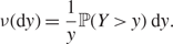
where W and Y represent random variables distributed like Wi and Yi, respectively. The Vervaat perpetuity has been much studied. Vervaat [Reference Vervaat19] showed that the random variable X is infinitely divisible, and obtained its Lévy–Khintchine representation. This is the basis of our simulation framework, and, furthermore, we show that, under the mild assumption that the Laplace transform of Y exists, X turns out to be a Lévy process with Lévy measure proportional to ℙ(Y >y)/y. There is also no loss of generality to consider only the case when Y >0, as it can be shown that a two-sided perpetuity can be split into the difference of two one-sided perpetuities. Goldie and Grübel [Reference Goldie and Grübel13] and Grübel and Rösler [Reference Grübel and Rösler14] studied the tails of these perpetuities. Random variables of this type also appear as the limit of shot noise processes [Reference Takács17], [Reference Takács18].
In this paper we are interested in exactly simulating a generalised Vervaat perpetuity. In the literature much attention has been paid to the special case when Yi =1 almost surely, in which X has the generalised Dickman distribution [Reference Arratia, Aldous and Propp1], [Reference Dickman9]. Even so, explicit expressions for the distribution of X are difficult to obtain. The first simulation method is based on a density approximation given in [Reference Devroye7]. Later, Devroye and Fawzi [Reference Devroye and Fawzi8] and Fill and Huber [Reference Fill and Huber12] used a dominated coupling from the past procedure for Markov chains. Cloud and Huber [Reference Cloud and Huber5] proposed an improvement by running both an upper and lower bound on the Markov chain. Chi [Reference Chi4] suggested an alternative approach based on a rejection sampling procedure. However, these algorithms are efficient only for the Dickman distribution, where the parameter t =1, and their speed slows down considerably when t becomes larger than 1.
We develop a faster and more efficient simulation algorithm for the generalised Dickman distribution with parameter t. Since it is viewed here as a Lévy process over the range of parameters t, with Lévy measure v(dy) = (1/y)1{y<1}, we thus call it the Dickman process. The paths of the Dickman process can be characterised by a marked renewal process where the renewal intervals are the hitting times of level 1, and the jumps are the overshoots at this time. By simulating its path along each hitting time of level 1, we obtain a simulation algorithm for the Dickman process. Similar to our method, the approach in [Reference Chi4] also utilises the truncated density of the perpetuity. However, the advantage of our algorithm is that it is based on a marked renewal process, which not only provides a pathwise probabilistic interpretation of the corresponding Lévy process, but also means that the incremental random variables we need to simulate are i.i.d. pairs, allowing us to employ vectorisation to reduce the total computation time. This is not the case for the algorithm suggested in [Reference Chi4], where the incremental variables depend on the previous variables. We provide comparisons of the simulation speed of our algorithm with the algorithms suggested in [Reference Chi4], [Reference Cloud and Huber5], [Reference Devroye and Fawzi8], and [Reference Fill and Huber12]. We found that our method outperforms the other algorithms and even more substantially when t is large.
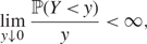
Blanchet and Sigman [Reference Blanchet, Sigman, Goldie and Mijatović2] proposed a modification of the dominated coupling from the past algorithm to sample from generalised Vervaat perpetuities. The algorithm imposes similar regularity conditions to ours on the density of Yi. However, it also requires Yi to have a heavy tail. In this paper we develop a framework for simulating from generalised Vervaat perpetuities. In particular, we prove a distributional decomposition result, which states that a generalised Vervaat perpetuity X can be represented as the sum of a gamma or truncated gamma process and independent compound Poisson processes. Thus, it can be sampled by generating each of these components separately and adding them up. The condition we need is
 \begin{equation}
\lim_{y\downarrow0}\frac{\mathbb{P}(Y<y)}{y}<\infty,
\end{equation}
which holds for a wide range of distributions, such as the gamma (shape parameter larger than 1), Pareto, Weibull (light tailed), beta, and normal distributions as well as all discrete distributions (to avoid technicalities 0 is not a possible value). Whenever a density exists, it should possess a finite derivative at 0.
Using the marked renewal representation, we develop an exact simulation algorithm for the truncated gamma process, which we define to be the Lévy process with Lévy measure
 $$\nu ({\rm{d}}y) = \frac{{{{\rm{e}}^{ - \mu y}}}}{y}{{\bf{1}}_{\{ y < b\} }}{\rm{d}}y$$
for some truncation level b. The truncated gamma process can be obtained from the gamma process by restricting the size of its jumps to be bounded from above by b. It is also a generalised Vervaat perpetuity with Yi ~ V ∧ 1, where V ~ Exp(μ). This algorithm is important, as it forms the basis of other algorithms for more general distributions of Yi. We provide specific examples to demonstrate the methodology, and present numerical results and graphical illustrations for the cases when Yi has a gamma distribution, and when Yi has a normal distribution.
This paper is organised as follows. In Section 2 we give a representation of the generalised Vervaat perpetuities as gamma-related processes. We also prove that a two-sided perpetuity is the difference of two positive perpetuities. In Section 3 we study the specific cases of a Dickman process and a truncated gamma process. The marked renewal path representation is described and the exact simulation algorithms developed. Numerical analysis and comparison with existing algorithms are provided. In Section 4 we prove the distributional decomposition result, which enables us to exactly simulate a generalised Vervaat perpetuity. Numerical examples are also given to demonstrate the accuracy and efficiency of our algorithms.
2. Generalised Vervaat perpetuities
We obtain the following distributional decomposition result for a positive perpetuity X > 0.
Theorem 2.1. Consider the generalised Vervaat perpetuity X with Yi > 0. We define the Laplace transforms  $\hat f(\beta ) = {\mathbb{E}}(\exp ( - \beta X))$ and
 $\hat g(\beta ) = {\mathbb{E}}(\exp ( - \beta Y_i ))$. Then we have
 $$\hat f(\beta ) = \exp ( - t\int_0^\infty {\frac{{1 - {e^{ - \beta y}}}}{y}} \mathbb{P}(Y > y)\rm{d}y).$$
Hence,  $X\mathop = \limits^D Z_t $, where Zt is a Lévy process with Lévy measure
 $$\nu ({\rm{d}}y) = \frac{1}{y}\mathbb{P}(Y > y)\, \rm{d}y.$$
Proof. For W = U 1/t, the density of W is twt −1. Then, from (1.2), we have
 \begin{equation*}
\skew5\hat{f}(\beta ) = \int_0^1 \skew5\hat{f}(\beta w)\skew5\hat{g}(\beta w)tw^{t-1}\rm{d} w,
\end{equation*}
and, therefore,
 $$\beta^t \skew5\hat{f}(\beta ) = \int_0^\beta \skew5\hat{f}(w)\skew5\hat{g}(w)tw^{t-1}\rm{d} w.$$
Differentiating with respect to β on both sides, we have
 $$
\frac{\mathrm{d}}{\mathrm{d}\beta }\skew5\hat{f}(\beta ) = -t\,\frac{1-\skew5\hat{g}(\beta )}{\beta }\skew5\hat{f}(\beta ) .
$$
Solving the first-order differential equation with respect to β, we obtain
 $$\hat f(\beta ) = \exp ( - t\int_0^\beta {\frac{{1 - \hat g(u)}}{u}} {\rm{du}}) = \exp ( - t\int_{\rm{0}}^\infty {\frac{{{\rm{1}} - {{\rm{e}}^{{\rm{ - }}\beta {\rm{y}}}}}}{{\rm{y}}}} \mathbb{P} ({\rm{Y}} > {\rm{y}}){\rm{dy}}),$$
and (2.1) follows. Thus,  $ X\mathop = \limits^D Z_t $, where Zt has Lévy measure defined in (2.2).
We can see that Zt is a gamma-related Lévy process with Lévy measure density proportional to ℙ(Y > y)/y −1. For a two-sided perpetuity, where Y takes values in the whole real line, the following result shows that it is the difference of two positive perpetuities and, thus, it suffices to study only positive perpetuities.
Corollary 2.1. Suppose now that ℙ(Y < 0) >0. Then
 $$\begin{array}{*{20}{l}}
{\hat f(\beta )}& = &{\exp ( - t(p\int_0^\infty {\frac{{1 - {{\rm{e}}^{ - \beta y}}}}{y}} \mathbb{P} (Y > y\mid Y > 0){\rm{dy}}}\\
{}&{}&{ + (1 - p)\int_0^\infty {\frac{{1 - {{\rm{e}}^{\beta y}}}}{y}} \mathbb{P} (Y < - y\mid Y < 0){\rm{dy}})),}
\end{array}$$
where p = ℙ(Y > 0).
Proof. For two-sided Y, the Laplace transform of the perpetuity X satisfies
 \begin{array}{*{20}{l}}
{\exp ( - t\int_0^\beta {\frac{{1 - \hat g(u)}}{u}{\mkern 1mu} } {\rm{d}}u)}\\
{\begin{array}{*{20}{l}}
{}& = &{\exp ( - t(\int_0^\beta {\int_0^\infty {\frac{{1 - {{\rm{e}}^{ - uy}}}}{u}} } \mathbb{P} (Y \in {\rm{d}}y){\mkern 1mu} {\rm{d}}u + \int_{\rm{0}}^\beta {\int_{\rm{0}}^\infty {\frac{{{\rm{1 - }}{{\rm{e}}^{{\rm{uy}}}}}}{{\rm{u}}}} } \mathbb{P} (Y \in {\rm{d}}( - {\rm{y}})){\mkern 1mu} {\rm{d}}u))}\\
{}& = &{\exp ( - t(\int_0^\beta {\int_0^\infty {{{\rm{e}}^{ - uy}}} } \mathbb{P} (Y > y){\mkern 1mu} {\rm{d}}y{\mkern 1mu} {\rm{d}}u + \int_{\rm{0}}^\beta {\int_{\rm{0}}^\infty {{{\rm{e}}^{{\rm{uy}}}}} } \mathbb{P} (Y < - {\rm{y}}){\mkern 1mu} {\rm{d}}y\, {\rm{d}}u))}\\
{}& = &{\exp ( - t(\int_0^\infty {\frac{{1 - {{\rm{e}}^{ - \beta y}}}}{y}} \mathbb{P} (Y > y){\mkern 1mu} {\rm{d}}y + {}\int_{\rm{0}}^\infty {\frac{{{\rm{1 - }}{{\rm{e}}^{\beta {\rm{y}}}}}}{y}} \mathbb{P} (Y < - y){\mkern 1mu} {\rm{d}}y))}\\
{}& = &{\exp ( - t(p\int_0^\infty {\frac{{1 - {{\rm{e}}^{ - \beta y}}}}{y}} \mathbb{P} (Y > y\mid Y > 0){\mkern 1mu} {\rm{d}}y}\\
{}&{}&{ + (1 - p)\int_0^\infty {\frac{{1 - {{\rm{e}}^{\beta y}}}}{y}} \mathbb{P} (Y < - y\mid Y < 0){\mkern 1mu} {\rm{d}}y)),}
\end{array}}
\end{array}
which is easily seen as the difference of two positive perpetuities, one with  ${W_i}\mathop = \limits^{\rm{D}} {\cal {U}^{1/pt}}$ and
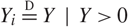 $Y_i \mathop = \limits^D Y|Y{\rm{ }} > {\rm{ }}0 $, and the other with
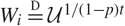 ${W_i}\mathop = \limits^{\rm{D}} {\cal{U}^{1/(1 - p)t}}$ and
 $ Y_i \mathop = \limits^D - Y|Y{\rm{ }} \lt {\rm{ }}0 $.
Our aim is to simulate the generalised Vervaat perpetuity X for a given distribution of Yi. In the simplest case when Yi =1 almost surely, X is known as the Vervaat perpetuity and it reduces to the Dickman process. When Yi ~ V, where V ~ Exp(μ), we obtain the gamma process with parameter μ, and when Yi ~ V ∧ 1, we obtain the truncated gamma process. Making use of a marked renewal representation for the paths, we develop fast and exact simulation algorithms for these perpetuities. These cases are important as they form the basis of the other algorithms. We will then give other examples to demonstrate how our methodology can be adapted to general random variables Yi. Our method works for any Yi satisfying (1.3).
3. Generalised Dickman distribution and the truncated gamma process
When Y ~ Exp(μ), we have ℙ(Y > y) = e−μy, and, thus,
 $$\hat f(\beta ) = \exp ( - t\int_0^\infty {(1 - {{\rm{e}}^{ - \beta y}})} \frac{1}{y}{{\rm{e}}^{ - \mu y}}{\rm{d}}y),$$
which is the Laplace transform of a gamma process with parameter μ. This can be simulated easily by sampling from the gamma distribution.
When Y =1 almost surely, we have ℙ(Y > y) = 1{y < 1}, and, thus,
 $$\hat f(\beta ) = \exp ( - t\int_0^1 {(\frac{{1 - {{\rm{e}}^{ - \beta y}}}}{y})} {\rm{d}}y),$$
which is the Laplace transform of a generalised Dickman distribution with parameter t. This is also a Lévy process Zt with Lévy measure (1/y)1{y<1}, and, hence, we call it the Dickman process.
When Y = V ∧ 1, where V ~ Exp(μ), we have ℙ(Y > y) = e−μy1{y < 1}, and, thus,
 $$\hat f(\beta ) = \exp ( - t\int_0^1 {(1 - {{\rm{e}}^{ - \beta y}})} \frac{{{{\rm{e}}^{ - \mu y}}}}{y}{\rm{d}}y),$$
which is the Laplace transform of a truncated gamma process with parameter μ. The truncated gamma process refers to the gamma process with truncated Lévy measure
 $$\frac{{{{\rm{e}}^{ - \mu y}}}}{y}{\bf{1}_{\{ y < 1\} }}.$$
To simulate the Dickman process and the truncated gamma process, we utilise a marked renewal process representation of its sample paths. We now describe the sample paths of truncated subordinators using a marked renewal process.
3.1. The marked renewal process
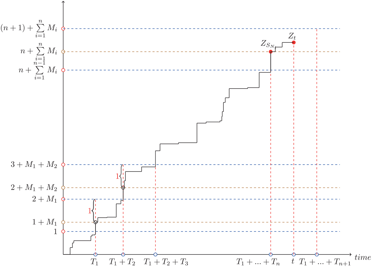
The paths of the truncated subordinator Zt can be characterised by a marked renewal process. First, we define a sequence of hitting times T 1, T 2, T 3, …, and defining 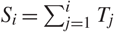 $S_i = \sum\nolimits_{j = 1}^i T_j$, let
 \begin{equation}
T_i\,:\,=\inf\{ t>S_{i-1}\mid Z_t>Z_{S_{i-1}}+1\}, \qquad i=2,3,\ldots.
\end{equation}
These T 1, T 2 … are treated as the holding times for the renewal process. We further define M 1,M 2, … to be the overshoots at time S 1, S 2, …, i.e.
 \begin{equation*}
M_i\,:\,= Z_{S_i}-Z_{S_{i-1}}-1.
\end{equation*}
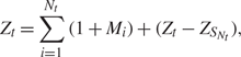
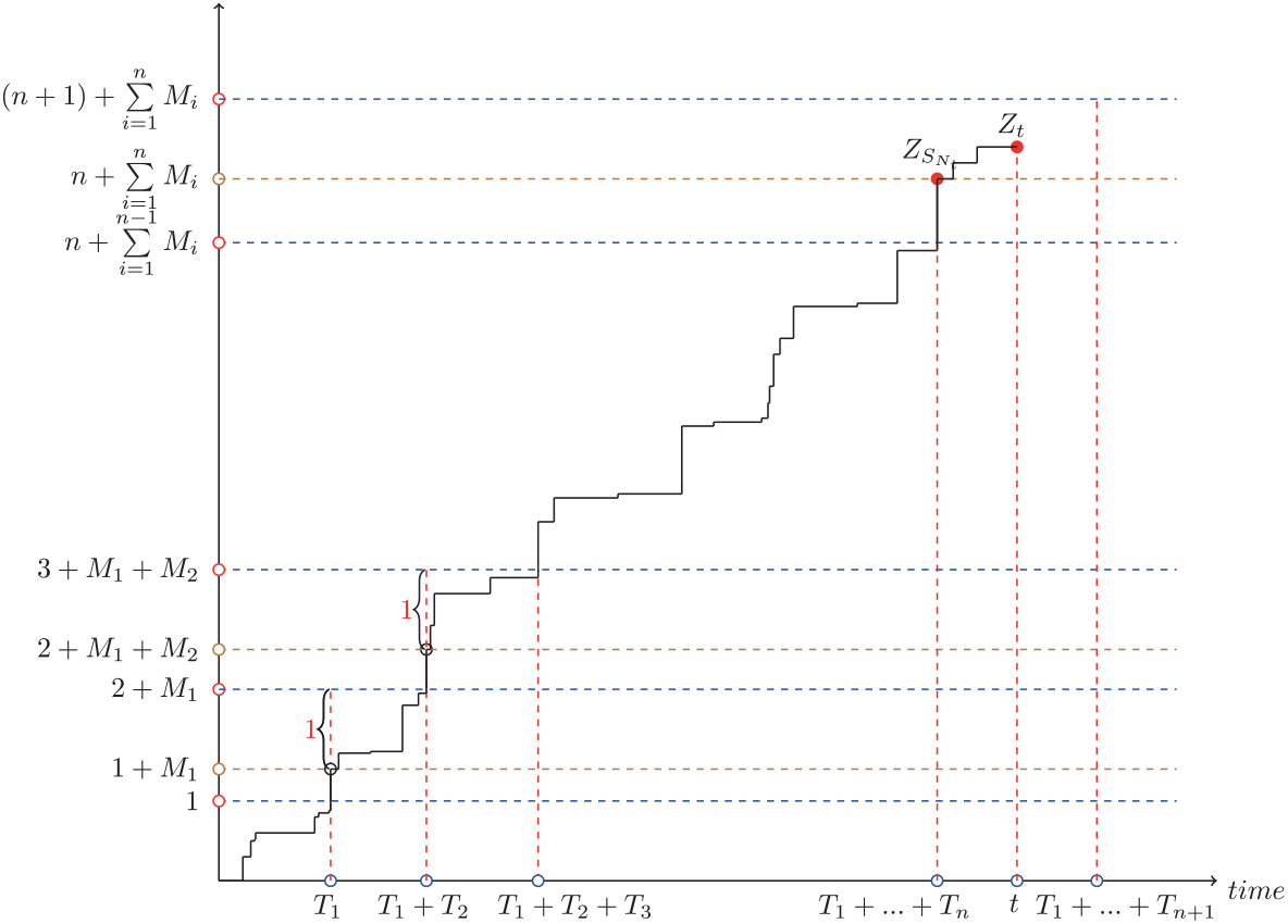
Hence, at time Si the process will increase by (1 + Mi) units for all i. Since the process Zt has independent and stationary increments, each pair of (Ti,Mi) are i.i.d. with joint density given in Theorem 3.1. In addition, Mi will be bounded by 0 and 1 for all i as the jump sizes of the process are restricted by 1. The value of the process at time Sn will be  $Z_{S_n } = \sum\nolimits_{i = 1}^n (1 + M_i )$. The position of the process Zt at time t can therefore be expressed as the sum of a marked renewal process with a random variable,
 \begin{equation}
Z_t= \sum_{i=1}^{N_t} (1+M_i)+ ( Z_{t}-Z_{S_{N_t}} ),\end{equation}
where  $N_t = \sum\nolimits_{i = 1}^\infty {\bf{1}}_{\{ S_i \le t\} }$ is the renewal process determined via (3.1) such that SN t ≤ t < SN t+1. We have
 $${Z_t} - {Z_{{S_{{N_t}}}}}\mathop = \limits^{\rm{D}} {Z_{t - {S_{{N_t}}}}}\mid {S_{{N_t} + 1}} > t\mathop = \limits^{\rm{D}} {Z_t}\mid T > t,$$
where the last equality is due to the strong Markov property of Zt.
We illustrate the marked renewal framework graphically in Figure 1. The sum in the first part of (3.2) represents the position of the truncated process at time SN t just before it reaches t. The second term in (3.2) represents the final movement of the process within time t −Nt. Thus, Zt can be simulated by generating pairs of hitting times and overshoots (Ti, Mi), stopping when the sum of Ti that have been generated, say SN t + 1, becomes larger than the input t. We then generate the final part {Zt | T > t} and return the entire sum (3.2).
Graphical illustration of a sample path of Zt.
3.2. Hitting times and overshoots
Now we obtain analytically the first hitting times and overshoots of the truncated gamma process and the Dickman process.
Theorem 3.1. Let T be the first hitting time of level 1 of a truncated gamma process Zt with μ ≥ 0, and let M be the overshoot at this time. Then the joint distribution of (T, M) is given by
 \begin{equation}
f_{T, M}(t,m)= \int_m^1 \frac{ \rm{e}^{\Gamma(0, \mu )t}\mu ^{t}}
{\Gamma(t)}y^{t-1} \frac{\rm{e}^{-\mu(1+m)}}{1+m-y}\rm{d} y
\quad\text{for }\mu>0,\end{equation}
where t ∈ (0,∞), m ∈ (0, 1). For the Dickman process, the joint density of (T, M) is the limit of (3.3) as μ→0,
 \begin{equation}
f_{T, M}(t,m)= \int_m^1 \frac{ \rm{e}^{-\gamma t}}{\Gamma(t)} \frac{ y^{t-1}}{1+m-y}\rm{d} y,
\end{equation}
where γ is the Euler–Mascheroni constant, t ∈ (0,∞), and m ∈ (0, 1).
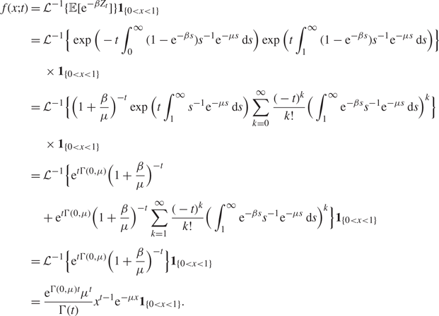
Proof. Let f (x;t) denote the density of Zt. For μ > 0, the density of Zt restricted to (0, 1) can be derived through its Laplace transform. We have
 $$\begin{array}{*{20}{l}}
{f(x;t)}& = &{{{\cal L}^{ - 1}}\{ \mathbb{E} [{{\rm{e}}^{ - \beta {{\rm{Z}}_{\rm{t}}}}}]\} {{\bf{1}}_{\{ 0 < x < 1\} }}}\\
{}& = &{{{\cal L}^{ - 1}}\{ \exp ( - t\int_0^\infty {(1 - {{\rm{e}}^{ - \beta s}})} {s^{ - 1}}{{\rm{e}}^{ - \mu {\rm{s}}}}{\rm{d}}s)\exp (t\int_{\rm{1}}^\infty {({\rm{1}} - {{\rm{e}}^{ - \beta s}})} {s^{ - {\rm{1}}}}{{\rm{e}}^{ - \mu s}}{\rm{d}}s)\} }\\
{}&{}&{ \times {{\bf{1}}_{\{ 0 < x < 1\} }}}\\
{}& = &{{{\cal L}^{ - 1}}\{ {{(1 + \frac{\beta }{\mu })}^{ - t}}\exp (t\int_1^\infty {{s^{ - 1}}} {{\rm{e}}^{ - \mu s}}{\rm{d}}s)\sum\limits_{{\rm{k = 0}}}^\infty {\frac{{{{( - t)}^k}}}{{k{\rm{!}}}}} {{(\int_{\rm{1}}^\infty {{{\rm{e}}^{ - \beta s}}{s^{ - {\rm{1}}}}{{\rm{e}}^{ - \mu s}}} {\rm{d}}s)}^k}\} }\\
{}&{} &{ \times {{\bf{1}}_{\{ 0 < x < 1\} }}}\\
{}& = &{{{\cal L}^{ - 1}}\{ {{\rm{e}}^{t\Gamma ({\rm{0}},\mu )}}{{({\rm{1 + }}\frac{\beta }{\mu })}^{ - t}}}\\
{}& {} &{ + {{\rm{e}}^{t\Gamma ({\rm{0}},\mu )}}{{({\rm{1 + }}\frac{\beta }{\mu })}^{ - t}}\sum\limits_{k{\rm{ = 1}}}^\infty {\frac{{{{( - t)}^k}}}{{k{\rm{!}}}}} {{(\int_{\rm{1}}^\infty {{{\rm{e}}^{ - \beta s}}{s^{ - {\rm{1}}}}{{\rm{e}}^{ - \mu s}}} {\rm{d}}s)}^k}\} {{\bf{1}}_{\{ {\rm{0}} < {\rm{x}} < {\rm{1}}\} }}}\\
{}& = &{{{\cal L}^{ - 1}}\{ {{\rm{e}}^{t\Gamma ({\rm{0}},\mu )}}{{({\rm{1 + }}\frac{\beta }{\mu })}^{ - {\rm{t}}}}\} {{\bf{1}}_{\{ {\rm{0}} < {\rm{x}} < {\rm{1}}\} }}}\\
{}& = &{\frac{{{{\rm{e}}^{\Gamma ({\rm{0}},\mu )t}}{\mu ^t}}}{{\Gamma (t)}}{x^{t - 1}}{{\rm{e}}^{ - \mu x}}{{\bf{1}}_{\{ {\rm{0}} < {\rm{x}} < {\rm{1}}\} }}.}
\end{array}$$
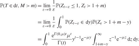
Using the strong Markov property of Lévy processes, we have
 \begin{array}{*{20}{l}}
{\mathbb{P} (T \in {\rm{d}}t,M > m)}&{ = \mathop {\lim }\limits_{\varepsilon \to 0} \frac{1}{\varepsilon } \mathbb{P} ({Z_{t - \varepsilon }} \le 1,{Z_t} > 1 + m)}\\
{}&{ = \mathop {\lim }\limits_{\varepsilon \to 0} \frac{1}{\varepsilon }\int_0^1 \mathbb{P} ({Z_{t - \varepsilon }} \in {\rm{d}y}) \mathbb{P} ({{\rm{Z}}_\varepsilon } > {\rm{1}} + m - y)}\\
{}&{ = \int_0^1 {\frac{{{{\rm{e}}^{\Gamma ({\rm{0}},\mu ){\rm{t}}}}{\mu ^{\rm{t}}}}}{{\Gamma (t)}}} {y^{t - 1}}{{\rm{e}}^{ - \mu {\rm{y}}}}\int_{{\rm{1 + }}m - y}^\infty {{z^{ - {\rm{1}}}}} {{\rm{e}}^{ - \mu {\rm{z}}}}{\rm{d}}z\,{\rm{d}}y.}
\end{array}
Differentiating (3.6) with respect to m, the joint density of (T, M) in (3.3) directly follows. For the Dickman process, we take the limit as μ→0. The density of Zt within (0, 1) is obtained by taking the limit of (3.5), i.e.
 \begin{equation}
f(x,t) = \lim_{\mu\to 0}\frac{ \rm{e}^{[\Gamma(0, \mu
)+\log(\mu)]t}}{\Gamma(t)}x^{t-1}\rm{e}^{-\mu x} = \frac{\rm{e}^{-\gamma
t}}{\Gamma(t)}x^{t-1}, \qquad 0<x<1,
\end{equation}
with γ being the Euler–Mascheroni constant. Hence, the associated distribution of (T, M) directly follows from (3.4).
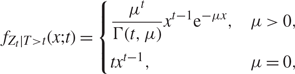
Given that the first passage time of Zt hitting level 1 is greater than t, the distribution of the truncated process Zt is characterised via its density within (0, 1). The details are as follows.
Theorem 3.2. The density of Zt | T > is given by
 $${f_{{Z_t}|T > t}}(x;t) = \left\{ {\begin{array}{*{20}{l}}
{\frac{{{\mu ^t}}}{{\Gamma (t,\mu )}}{x^{t - 1}}{{\rm{e}}^{ - \mu {\rm{x}}}},}&{\mu > 0,}\\
{t{x^{t - 1}},}&{\mu = 0,}
\end{array}} \right.$$
where 0 < x < 1.
Proof. We know that
 $${Z_t}\mid T > t{\rm{ }}\mathop = \limits^{\rm{D}} {Z_t}\mid {Z_t} < 1,$$
since {T > t} is equivalent to {Zt < 1}. The density therefore satisfies
 $${f_{{Z_t}\mid T > t}}(x;t) = {f_{{Z_t}\mid {Z_t} < 1}}(x;t) = \frac{{f(x;t)}}{{\int_0^1 f (x;t){\rm{d}}x}}.$$
Thus, the density immediately follows from (3.8).
3.3. Exact simulation of the generalised Dickman distribution
Based on the marked renewal framework and choosing suitable acceptance–rejection (A/R) envelopes for fT,M(t, m) and fZ t | T>t(x;t), we have the following simulation algorithm for the Dickman process, or, equivalently, the generalised Dickman distribution.
Algorithm 3.1. (Simulation of the Dickman process (generalised Dickman distribution).)
1. Set S = 0, γ = −digamma(1).
2. Generate (T, M) via the following steps.
(a) Generate
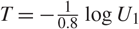
 $U_1 \sim {\cal U}(0,1)$, and set $T = - {\textstyle{1 \over {0.8}}}\log U_1$.
(b) Generate Y ~ Beta(T, 0.5),
$U_2 \sim {\cal U}(0,1)$, and set
$$
M=Y-1+(1-Y)\exp ( - U_2\log (1-Y) ) .
$$
(c) Generate
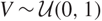
$V \sim {\cal U}(0,1)$, and if
(3.9)\begin{equation}
V \le \frac{1}{2.35}\frac{\Gamma (0.5)\rm{e}^{-(\gamma -0.8)T}}{0.8\Gamma (T+0.5)}\frac{( -\log (1-Y))}{(1-Y)^{-0.5}},
\end{equation}
then accept (T, M). Otherwise, reject this candidate and go back to step 2(a).
3. If T > t, continue to step 4. Otherwise, set S = S + 1 + M, t = t − T, and go back to step 2.
4. Generate
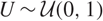
$U \sim {\cal U}(0,1)$ and set X = U 1/t.5. Return S + X.




Proof. For the joint density fT, M(t, m), we simulate (T, M, Y) jointly from the integral in (3.4),
 $$f(t,m,y) = \frac{{{{\rm{e}}^{ - \gamma t}}{y^{t - {\rm{1}}}}}}{{\Gamma (t)}}\frac{1}{{1 + m - y}}$$
for t ∈ (0,∞), 0 < m < y < 1. The A/R envelope chosen is
 \begin{equation}
g(t,m,y)=\sigma \rm{e}^{-\sigma t}\frac{\Gamma (t+\eta )}{\Gamma
(t)\Gamma (\eta )}y^{t-1}(1-y)^{\eta -1}\frac{{1}/{(1+m-y)}}{(-\log (1-y))},
\end{equation}
where σ = 0.8 and η = 0.5 are chosen numerically via two-dimensional optimisation. Furthermore, fZ t | T > t(x;t) can be simulated directly via inverse transformation resulting in step 4.
3.4. Exact simulation of the truncated gamma process
For the truncated gamma process, we could generate a Dickman process and apply a final A/R scheme. However, the algorithm is not very efficient, especially for large μ as the acceptance rate is exponentially decreasing in μ. Thus, we propose the following algorithm based on the marked renewal framework to sample a truncated gamma process.
Algorithm 3.2. (Simulation of the truncated gamma process (marked renewal approach).)
1. Set S = 0.
2. Generate (T, M) via the following steps.
(a) Numerically minimise
\begin{array}{l}
C(\vartheta ,\delta )\\
\quad = \frac{{\Gamma (\delta ){{\rm{e}}^{ - \mu }}}}{{\vartheta (1 - \delta )e}}\\
\quad \quad \times \frac{{{{\rm{e}}^{\Gamma ({\rm{0}},\mu )\exp (\Gamma ({\rm{0}},\mu ){\rm{ + }}\vartheta {\rm{ + }}\log (\mu ))}}{\mu ^{\exp (\Gamma ({\rm{0}},\mu ){\rm{ + }}\vartheta {\rm{ + }}\log (\mu ))}}{{\rm{e}}^{\vartheta \exp (\Gamma ({\rm{0}},\mu ){\rm{ + }}\vartheta {\rm{ + }}\log (\mu ))}}}}{{\Gamma (\exp (\Gamma (0,\mu ) + \vartheta + \log (\mu )) + \delta )}},
\end{array}
record the optimal value ϑ ∗ and δ ∗, and set C = C(ϑ ∗, δ ∗).
(b) Generate
$U_1 \sim {\cal U}(0,1)$ and set T = −log (U 1)/ϑ ∗.(c) Generate Y ~ Beta(T, δ ∗),,
$U_2 \sim {\cal U}(0,1)$, and set
$$
M=Y-1+(1-Y)\exp ( - U_2\log (1-Y) ) .
$$
(d) Generate
$V_1 \sim {\cal U}(0,1)$. If
(3.11)\begin{equation}
V_1\le \frac{1}{C} \frac{\Gamma(\delta^*)}{\vartheta^*}\frac{\rm{e}^{\Gamma(0,\mu)T}\mu^{T} \rm{e}^{\vartheta^* T}}{\Gamma(T+\delta^*)}\frac{-\log(1-Y)}{(1-Y)^{\delta^*-1}}\rm{e}^{-\mu(1+M)},
\end{equation}
then accept (T, M). Otherwise, reject this candidate and go back to step 2(b).
3. If T >t, continue to step 4. Otherwise, set S = S +1+M, t = t −T, and go back to step 2.
4. Generate X via the following steps.
(a) Generate
$U_3 \sim {\cal U}(0,1)$ and set $X = U_3^{1/t}$.(b) Generate
$V_2 \sim {\cal U}(0,1)$. If
${V_2} \le \exp \,( - \mu X),$
then accept X. Otherwise, reject this candidate and go back to step 4(a).
5. Return S + X.










Proof. For the joint density fT, M(t, m), we simulate (T, M, Y) jointly from the integral in (3.3),
 \begin{equation
f(t,m,y)=\frac{
y^{t-1}\frac{\r
\end{equation*}
where t ∈ (0,∞), 0 < m < y < 1. We choose the envelope
 $$g(t,m,y) = \vartheta {{\rm{e}}^{ - \vartheta {\rm{t}}}}\frac{{\Gamma ({\rm{t}} + \delta )}}{{\Gamma ({\rm{t}})\Gamma (\delta )}}{{\rm{y}}^{t - {\rm{1}}}}{({\rm{1}} - y)^{\delta - {\rm{1}}}}\frac{{{\rm{1/}}({\rm{1}} + m - y)}}{{[ - \log \,({\rm{1}} - y)]}}.$$
The ratio of the densities is bounded by
 \begin{equation}
\frac{f(t,m,y)}{g(t,m,y)} \le \frac{\Gamma(\delta)\rm{e}^{-\mu}}
{\alpha(1-\delta)e}\frac{\rm{e}^{\Gamma(0,\mu)t^*}\mu^{t^*} \rm{e}^{\alpha
t^*}}{\Gamma(t^*+\delta)}\,:=C(\vartheta, \delta),
\end{equation}
which we obtained by maximising the ratio with respect to t,
 \begin{equation*}
t^* = \exp\Big( \Gamma(0,\mu)+\alpha+\log(\mu)+\mathcal{O} \Big(
\frac{1}{t^*}\Big)\!\Big)\approx\exp( \Gamma(0,\mu)+\alpha+\log(\mu)).
\end{equation*}
We then minimise C(ϑ, δ) with respect to ϑ and δ via two-dimensional numerical optimisation. Finally, {Zt | T >t} can be simulated directly via an A/R scheme by choosing an envelope with density
 $$g(x;t)= \frac{x^{t-1}}{t}\mathbf{1}_{\{0<x<1\}}.$$
3.5. Numerical results
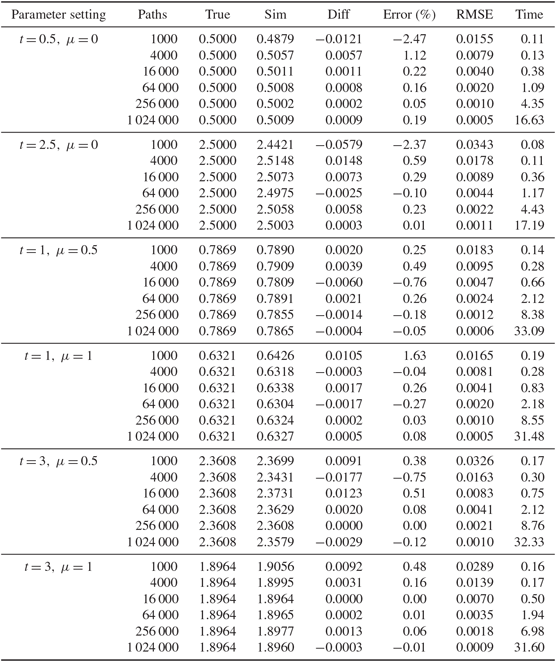
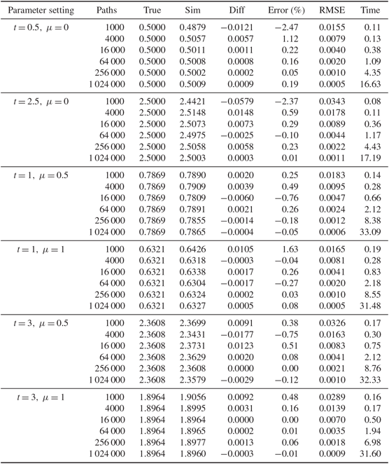
In this section we present some numerical results of the exact simulation methods developed in Algorithms 3.1 and 3.2. Numerical validation and tests for our simulation algorithms are all based on the true mean. The associated errors are reported by the difference, the percentage errors, and root mean square error (RMSE) (calculated as  $RMSE = \sqrt {SE^2 + Bias^2 }$). The detailed numerical results are reported in Table 1. We can see that each algorithm can achieve a very high level of accuracy, which is reflected by the difference in the theoretical mean and associated percentage errors. The simulation time is measured by the elapsed CPU time in seconds. We can see that both algorithms perform well. In particular, for Algorithm 3.2, the simulation time to generate the truncated gamma process is not highly influenced by μ.
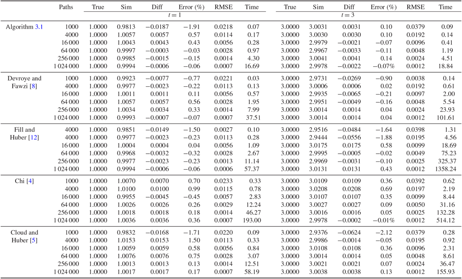
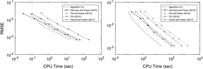
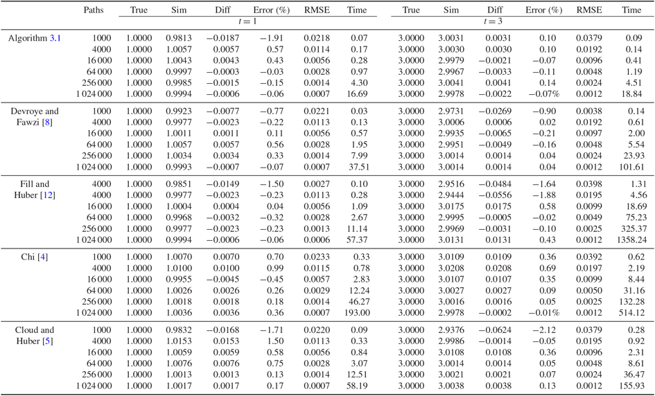
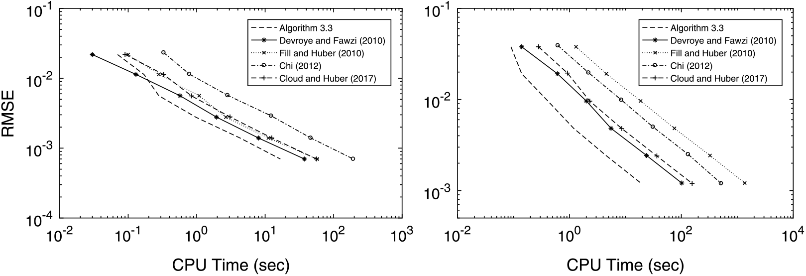
For the generalised Dickman distribution, we implement a comparison between Algorithm 3.1 against the algorithms suggested by Devroye and Fawzi [Reference Devroye and Fawzi8], Fill and Huber [Reference Fill and Huber12], Chi [Reference Chi4], and Cloud and Huber [Reference Cloud and Huber5]. The detailed numerical results based on different parameter settings against t are reported in Table 2 and the associated log-log plots for the RMSE against the CPU time are presented in Figure 2. In addition, we also compared the computation time to generate 100 000 samples using these five algorithms for different values of t, the details of which are presented in Table 3. We can see that sampling based on Algorithm 3.1 is much faster than algorithms in Devroye and Fawzi [Reference Devroye and Fawzi8], Fill and Huber [Reference Fill and Huber12], Chi [Reference Chi4], and Cloud and Huber [Reference Cloud and Huber5]. For instance, when t = 3, Algorithm 3.1 is four times faster than Devroye and Fawzi [Reference Devroye and Fawzi8], 50 times faster than Fill and Huber [Reference Fill and Huber12], 25 times faster than Chi [Reference Chi4], and seven times faster than Cloud and Huber [Reference Cloud and Huber5]. Compared with the other algorithms, the main advantage of Algorithm 3.1 is that the incremental random variables (Ti, Mi)i≥0 are i.i.d. pairs, and this means that we can employ vectorisation to reduce total computation time, especially for large values of t. Although the expected simulation time is unbounded for Algorithm 3.1, the simulation idea based on the marked renewal approach still outperforms the dominated coupling approach and rejection sampling approach, and even more so when t is large.
Comparisons between Algorithm 3.1 and the algorithms suggested in Devroye and Fawzi [Reference Devroye and Fawzi8], Fill and Huber [Reference Fill and Huber12], Chi [Reference Chi4], and Cloud and Huber [Reference Cloud and Huber5] for t =1 and t =3..
Convergence analysis of Algorithm 3.1 and the algorithms suggested in Chi [Reference Chi4], Cloud and Huber [Reference Cloud and Huber5], Devroye and Fawzi [Reference Devroye and Fawzi8], and Fill and Huber [Reference Fill and Huber12] for t =1 and t =3, respectively, with associated detailed numerical results reported in Table 2.
4. More general Vervaat perpetuities
In this section we present a general method for simulating Vervaat perpetuities for more general random variables Y. This method is applicable to a wide range of distributions, and we give several examples to demonstrate this. We have the following result, which decomposes the Vervaat perpetuity X into the sum of a gamma process (or truncated gamma process) and compound Poisson processes. For simplicity, we will let Y have a continuous density g.
Comparisons of the CPU times in seconds for the algorithms suggested in Chi [Reference Chi4], Cloud and Huber [Reference Cloud and Huber5], Devroye and Fawzi [Reference Devroye and Fawzi8], and Fill and Huber [Reference Fill and Huber12], with Algorithm 3.1 for 100 000 replications.

Lemma 4.1. Consider a perpetuity X defined in (1.1), with Y ∈ ℝ+. If the density of Y satisfies (1.3) then there exists K ∈ ℝ+ and b ∈ ℝ+ such that ℙ(Y > y) ≥ e−ky for all y < b. We then have the following two cases.
Case 1. There exists K ∈ ℝ+ such that ℙ(Y > y) ≥ e−ky for all Y ∈ ℝ+. Then we have
 \begin{equation}
B=\int_0^\infty \frac{\mathbb{P}(Y> y)-\rm{e}^{-ky}}{y}\rm{d} y<
\infty,
\end{equation}
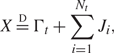
and, thus,
 $$X\mathop = \limits^{\rm{D}} {\Gamma _t} + \sum\limits_{i = 1}^{{N_t}} {{J_i}} ,$$
where
• Гt is a gamma process such that Гt ~ Г(t, k);
•
$\sum\nolimits_{i = 1}^{N_t } J_i$ is a compound Poisson process such that
• Nt is a Poisson process with rate tB;
• {Ji}i = 1,2, … are i.i.d. jumps with density
\begin{equation}
g_{J_i}(y) = \frac{\mathbb{P}(Y\ge y)-\rm{e}^{-ky}}{B y}, \qquad y\in \mathbb{R}^+.\nonumber
\end{equation}


Case 2. There only exists k ∈ ℝ+ such that ℙ (Y > y) ≥ e−ky for y < b. Then we have
 \begin{equation}
D=\int_0^b \frac{\mathbb{P}(Y> y)-\rm{e}^{-ky}}{y}\rm{d} y<\infty,
\end{equation}
and, thus,
 $$X\mathop = \limits^{\rm{D}} {Z_t} + \sum\limits_{i = 1}^{N_t^1} {J_i^{(1)}} + \sum\limits_{k = 1}^{N_t^2} {J_k^{(2)}} ,$$
where
• Zt is a truncated Gamma process with Lévy measure
$$
\nu(\mathrm{d}z) = z^{-1} \rm{e}^{-k z}\mathbf{1}_{\{ 0<z<b\}} \rm{d} z;
$$
•
$\sum\nolimits_{i = 1}^{N_t^1 } J_i^{(1)}$ is a compound Poisson process such that
•
$N_t^1$ is a Poisson process with rate tD;•
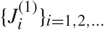
$\{ J_i^{(1)} \} _{i = 1,2, \ldots }$ are i.i.d. jumps with density
\begin{equation}
g_{J_i^{(1)}}(y) = \frac{\mathbb{P}(Y\ge y)-\rm{e}^{-ky}}{D y}, \qquad y\in (0, b);\nonumber
\end{equation}
•
$\sum\nolimits_{k = 1}^{N_t^2 } J_k^{(2)}$ is a compound Poisson process such that
•
$N_t^2$ is a Poisson process with rate tE, where
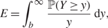
(4.5)\begin{equation}
E=\int_b^\infty \frac{\mathbb{P}(Y\ge y)}{y}\rm{d} y ,
\end{equation}
•
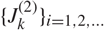
$\{ J_k^{(2)} \} _{i = 1,2, \ldots }$ are i.i.d. jumps with density
\begin{equation}
g_{J_k^{(2)}}(y) = \frac{\mathbb{P}(Y\ge y)}{E y}, \qquad y\in (b, \infty).
\end{equation}





Proof. If the density of Y satisfies (1.3) then g(0) < ∞. Hence, the survival function of Y, ℙ (Y > y) decays at an exponential rate or slower at 0. This implies that there exists a k ∈ ℝ+ such that ℙ (Y > y) ≥ e−ky for all y < b for some b ∈ ℝ+.
Case 1. If, furthermore, there exists such k ∈ ℝ+ so that ℙ (Y > y) ≥ e−ky holds for all y ∈ ℝ+, then, for B defined as in (4.1), it follows that the integral B is finite since
 \begin{equation}
\int_0^\infty \frac{\mathbb{P}(Y>y)-\rm{e}^{-ky}}{y}\rm{d} y = \int_0^1 \frac{\mathbb{P}(Y>y)-\rm{e}^{-ky}}{y}\rm{d} y +\int_1^\infty \frac{\mathbb{P}(Y>y)-\rm{e}^{-ky}}{y}\rm{d} y .\nonumber
\end{equation}
The second term is finite since we have assumed that the mean of Y exists, and we also have
 \begin{align*}
\int_0^1 \frac{\mathbb{P}(Y>y)-\rm{e}^{-ky}}{y}\rm{d} y & = [ \log y (
\mathbb{P}(Y>y)-\rm{e}^{-ky})]_0^1 +\int_0^1 \log y\Big(
g(y)-\frac{\rm{e}^{-ky}}{k}\Big)\rm{d} y \\ & = \int_0^1 \log
y\Big( g(y)-\frac{\rm{e}^{-ky}}{k}\Big)\rm{d} y \\ &<\infty,
\end{align*}
since g(0) < ∞. Hence, the Laplace transform of X can be expressed as
 \begin{array}{*{20}{l}}
{\mathbb{E} [{{\rm{e}}^{ - \beta {\rm{X}}}}]}& = &{\exp ( - {\rm{t}}\int_{\rm{0}}^\infty {({\rm{1}} - {{\rm{e}}^{ - \beta y}})} \frac{{{{\rm{e}}^{ - ky}}}}{y}{\rm{d}}y)}\\
{}&{}&{ \times \exp ( - tB\int_{\rm{0}}^\infty {({\rm{1}} - {{\rm{e}}^{ - \beta y}})} \mathbb{P} \frac{{(Y > y) - {{\rm{e}}^{ - ky}}}}{{By}}{\rm{d}}y)}\\
{}& = &{\mathbb{E} [{{\rm{e}}^{ - \beta {\Gamma _t}}}] \mathbb{E} [{{\rm{e}}^{ - \beta \sum\nolimits_{i = 1}^{{N_t}} {{J_i}} }}],}
\end{array}
and we have the distributional decomposition result given in (4.2).
Case 2. In the case where we only have ℙ (Y > y) ≥ e−ky for y < b for some b ∈ ℝ+, we define the integral D as in (4.3) and E as in (4.5). An argument similar to that above shows that they are finite, and we thus have
 \begin{array}{*{20}{l}}
{\mathbb{E} [{{\rm{e}}^{ - \beta {\rm{X}}}}]}& = &{\exp ( - t\int_{\rm{0}}^{\rm{b}} {({\rm{1}} - {{\rm{e}}^{ - \beta y}})} \mathbb{P} \frac{{(Y > y)}}{y}{\rm{d}}y)}\\
{}&{}&{ \times \exp ( - {\rm{t}}\int_{\rm{b}}^\infty {({\rm{1}} - {{\rm{e}}^{ - \beta y}})} \mathbb{P} \frac{{(Y > y)}}{y}{\rm{d}}y)}\\
{}& = &{\exp ( - {\rm{t}}\int_{\rm{0}}^b {({\rm{1}} - {{\rm{e}}^{ - \beta y}})} \frac{{{{\rm{e}}^{ - ky}}}}{y}{\rm{d}}y)}\\
{}&{}&{ \times \exp ( - tD\int_{\rm{0}}^b {({\rm{1}} - {{\rm{e}}^{ - \beta y}})} \mathbb{P} \frac{{(Y > y) - {{\rm{e}}^{ - ky}}}}{{Dy}}{\rm{d}}y)}\\
{}&{}&{ \times \exp ( - tE\int_b^\infty {({\rm{1}} - {{\rm{e}}^{ - \beta y}})} \mathbb{P} \frac{{(Y > y)}}{{Ey}}{\rm{d}}y)}\\
{}& = &{\mathbb{E} [{{\rm{e}}^{ - \beta {Z_t}}}]\mathbb{E}[{{\rm{e}}^{ - \beta \sum\nolimits_{i{\rm{ = 1}}}^{N_t^{\rm{1}}} {J_i^{({\rm{1}})}} }}]\mathbb{E}[{{\rm{e}}^{ - \beta \sum\nolimits_{k{\rm{ = 1}}}^{N_t^{\rm{2}}} {J_k^{({\rm{2}})}} }}].}
\end{array}
The distributional decomposition result (4.4) thus follows.
We now have a general method for exactly simulating generalised Vervaat perpetuities for a wide range of distributions for Y. In particular, case 2 is useful when the distribution of Y has finite support, or when Y has a tail which decays faster than exponential decay, in which case there does not exist k ∈ ℝ+ such that ℙ (Y > y) ≥ e−ky for all y. In the rest of this section, we give some examples to demonstrate the methodology.
Example 1. Let Y ~ Pareto(α, σ) From Theorem 2.1, the Laplace transform of X is
 $$\mathbb{E} [{{\rm{e}}^{ - \beta X}}] = \exp ( - t\int_{\rm{0}}^\infty {\frac{{{\rm{1}} - {{\rm{e}}^{ - \beta y}}}}{y}{\rm{d}}y} )\exp \left( { - t\int_\sigma ^\infty {\frac{{{\rm{1}} - {{\rm{e}}^{ - \beta y}}}}{y}{{\left( {\frac{\sigma }{y}} \right)}^\alpha }{\rm{d}}y} } \right).$$
Hence, 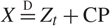 $ X\mathop = \limits^D Z_t + {\rm{CP}} $, where Zt ~ Dickman process and CP is a compound Poisson process, independent of each other. The Dickman process can be generated using Algorithm 3.1, and the compound Poisson process can be easily generated via an A/R scheme.
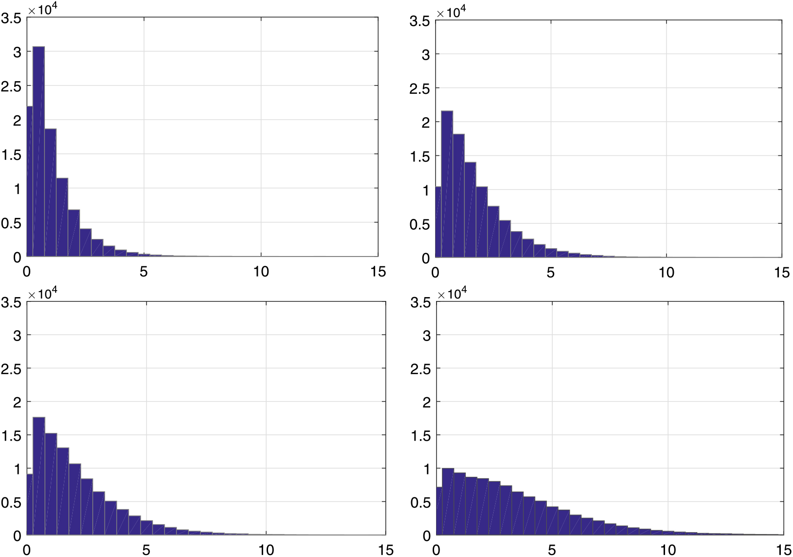
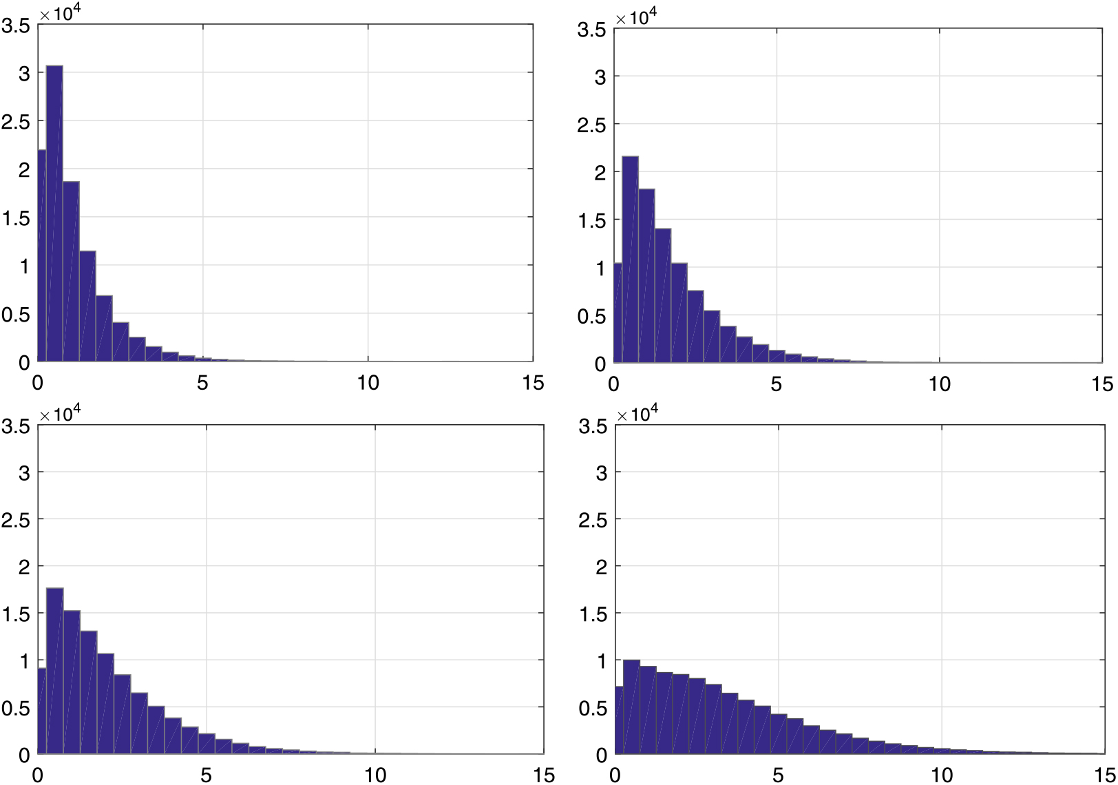
Example 2. Let Y ~ Gamma(α, β). Since g(0) < ∞ for all α ≥ 1, we can simulate all gamma perpetuities with α ≥ 1 and all values of β. Furthermore, for all α ≥ 1, there exists a k such that ℙ (Y > y) ≥ e−ky for all y; hence, it falls under case 1 of Lemma 4.1. Thus, the gamma perpetuity X can be split into 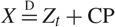 $ X\mathop = \limits^D Z_t + {\rm{CP}} $, where Zt is a gamma process and CP is a compound Poisson process independent of Zt by Lemma 4.1. In Figure 3 we show the histograms of the Vervaat perpetuity X for Y ~ Г(α, β) with different shape parameters α.
Histograms of perpetuity X with Y ~ Г(α, β) under the parameter setting α =1, 1.5, 2, 2.5 and β = 1.
Example 3. Let Y ~ Weibull(κ, λ). Since g(0) < ∞ for all κ ≥ 1, we can simulate all Weibull perpetuities with κ ≥ 1 and all values of λ. Furthermore, there only exists a k such that ℙ (Y > y) ≥ e−ky for y ∈ (0, b) for some b ∈ ℝ+. Hence, the perpetuity falls into case 2 of Lemma 4.1, and can be split into  $ X\mathop = \limits^D Z_t + {\rm{CP}}_{\rm{1}} + {\rm{CP}}_{\rm{2}} $, where Zt is a truncated gamma process, and CP1 and CP2 are compound Poisson processes, independent of each other and Zt. The truncated gamma process can be generated using Algorithm 3.2 and the two compound Poisson processes can be easily generated via A/R schemes.
Example 4. Let Y ~ Beta(α, β). Since g(0) < ∞ for all α ≥ 1, we can simulate all beta perpetuities with α ≥ 1 and all values of β. Furthermore, since the distribution has a finite support, there only exists a k such that ℙ (Y > y) ≥ e−ky for y ∈ (0, b) for some b ∈ ℝ+. Hence, the perpetuity falls into case 2 of Lemma 4.1, and the Lévy measure needs to be truncated. The beta perpetuity can be split into  $ X\mathop = \limits^D Z_t + {\rm{CP}}_{\rm{1}} + {\rm{CP}}_{\rm{2}}$ according to Lemma 4.1, where Zt is a truncated gamma process, and CP1 and CP2 are two compound Poisson processes, independent of each other and Zt.
Example 5. Let Y ~ Normal (μ, σ 2). The normal perpetuity X is two sided. According to Corollary 2.1, one could sample independent X 1 and X 2 each of which are half-normal perpetuities, and the difference X 1 – X 2 is the realisation of the two-sided perpetuity X.
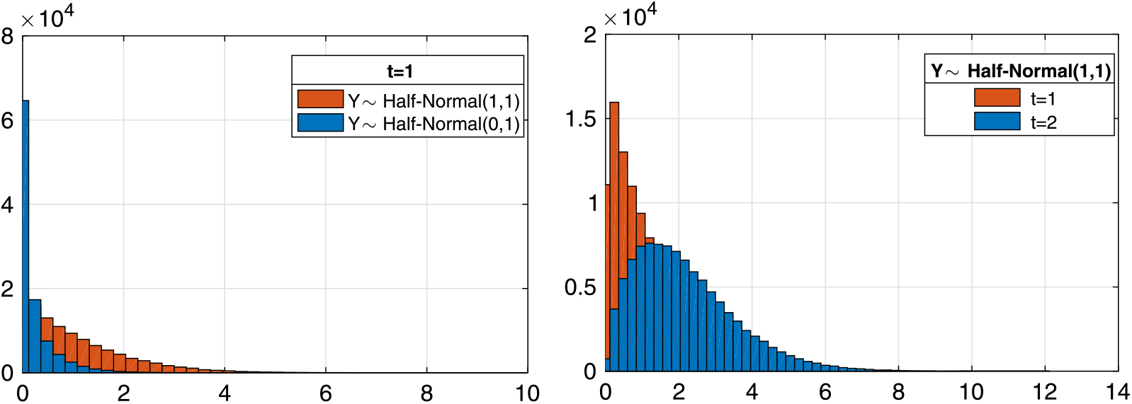
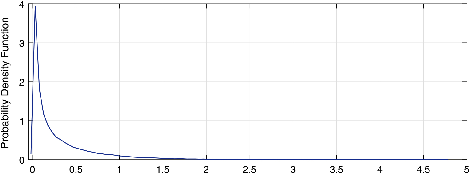
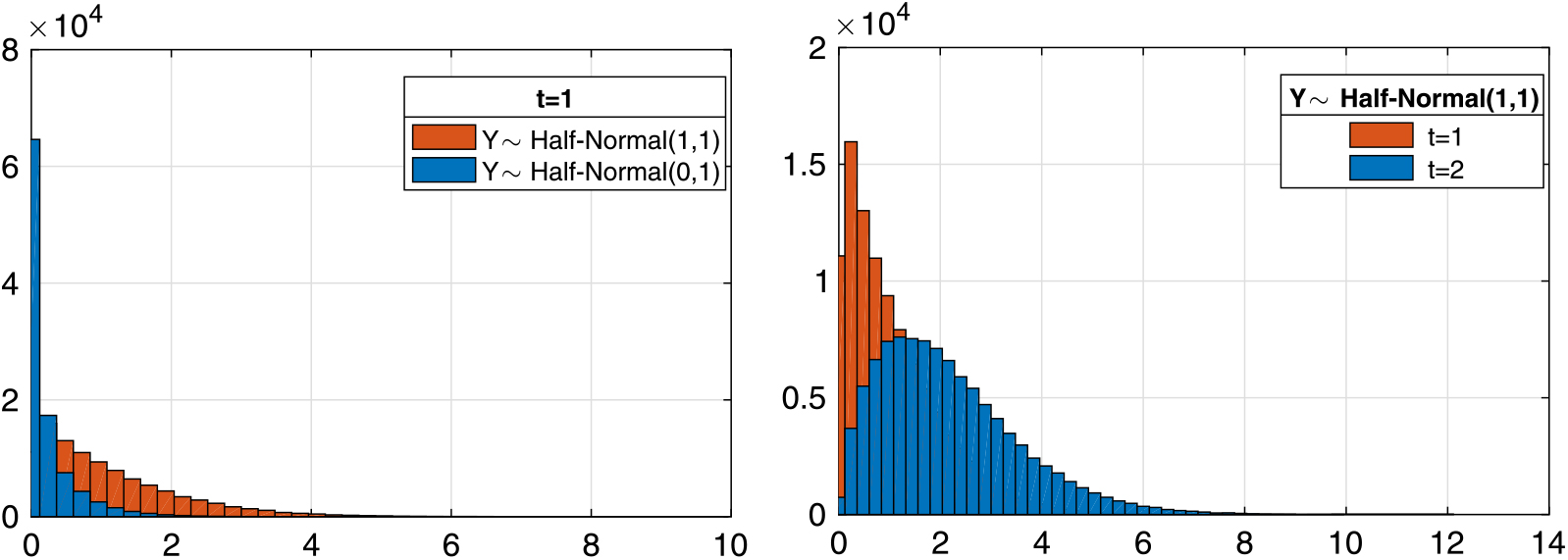
For a half-normal perpetuity Xi, where Yi ~ half-normal(μ, σ), there only exists a k such that ℙ(Y > y) ≥ e−ky for y ∈ (0, b) for some b ∈ ℝ+. Hence, the perpetuity Xi falls into case 2 and can be split into a truncated gamma process and two compound Poisson processes according to Lemma 4.1. The truncated gamma process can be generated via Algorithm 3.2 and the two compound Poisson processes can be easily generated via A/R schemes. In Figure 4 we illustrate a sample density plot for the perpetuity Xi with Yi ~ half-normal(0, 1). In Figure 5 we compare the distribution of Xi under different parameter settings.
Probability density function of perpetuity Xi with Yi ~ half-normal(0, 1).
Histograms of perpetuity Xi with Yi ~ half-normal(0, 1) and Yi ~ half-normal(1, 1) with t = 1, 2.
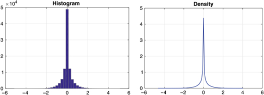
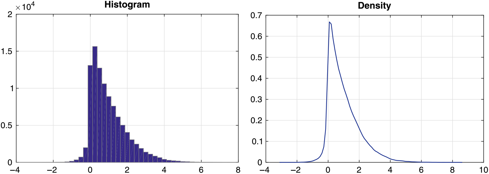
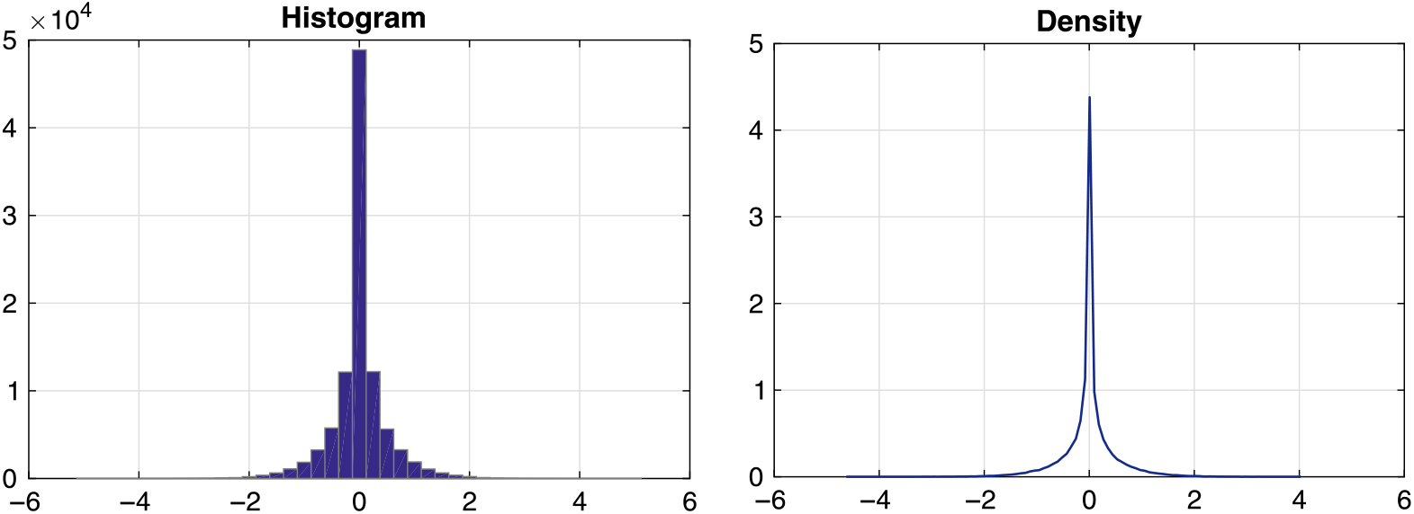
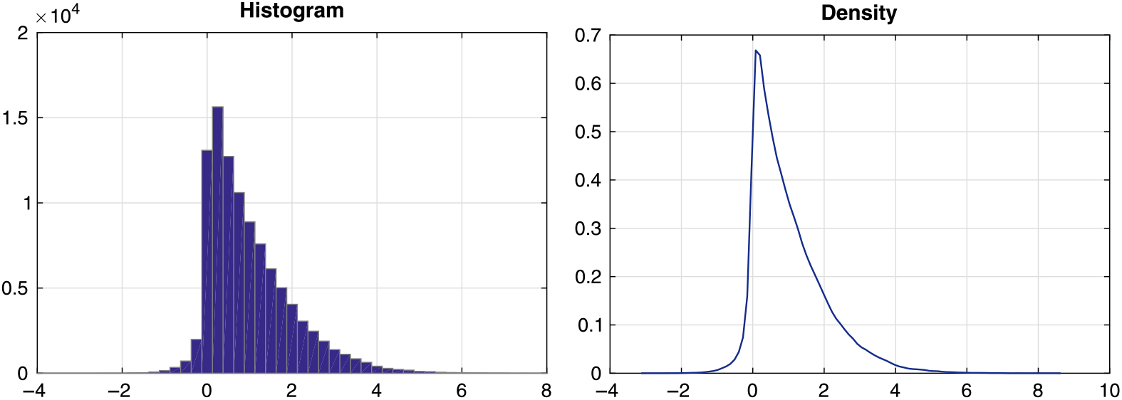
Now we can simulate the normal perpetuity X by generating two independent half-normal perpetuities X 1 and X 2 and taking the difference 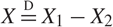 $ X\mathop = \limits^D X_1 {\rm{ }} - {\rm{ }}X_{\rm{2}} $. In Figures 6 and 7 we demonstrate the distribution behaviour of the two-sided perpetuity X via its histogram and density plot. We can also obtain other variations of the normal perpetuities by introducing a new variable B ~ Bernoulli(p) and setting
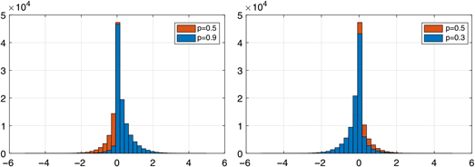
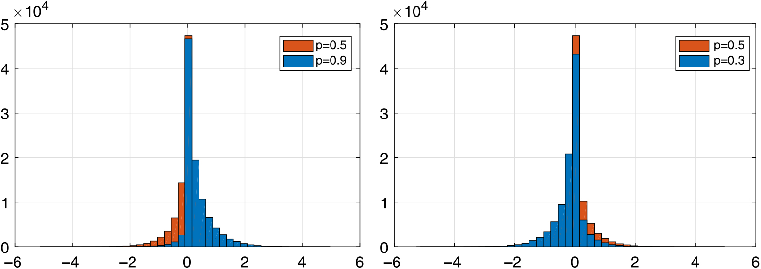
 $ \hat X\mathop = \limits^D pX_1 {\rm{ }} - (1 - p){\rm{ }}X_{\rm{2}} $. When
 $ p = {\textstyle{1 \over 2}}$ and Xi ~ Normal(0, 1), this is identical to the Normal(0, 1), perpetuity. In Figure 8 we illustrate the differences of the perpetuity X̂ and X in terms of their histograms.
Histogram and density plot of perpetuity X with Y ~ Normal(0, 1).
Histogram and density plot of perpetuity X with Y ~ Normal(1, 1).
Histogram of perpetuity X̂ = BX 1 – (1 – B)X 2 with B ~ Bernoulli(p) under parameter setting p = 0.3, 0.5, 0.9.
Acknowledgements
The authors would like to thank the Associated Editor and two reviewers for many constructive comments that greatly improved the presentation of our results.