2 Formulation of the problem

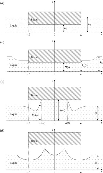
Let us assume that a rectangular prismatic channel with a horizontal bottom which is filled by an incompressible liquid with a partly immersed rectangular beam of length  $2L$ whose width coincides with the channel width and whose upper and lower planes are parallel to the channel bottom (figure 1 a). We assume that the channel is not limited by length. At the time $t<0$ , the liquid and the beam are at rest. Let us introduce a Cartesian coordinate system whose origin is on the channel bottom, the $x$ axis is directed along the channel and the $z$ axis is directed vertically upward, normal to the channel bottom. Let us assume that the $z$ axis passes through the beam centre; therefore, the beam edges have the coordinates $-L$ and $L$ on the $x$ axis. The initial depth of the liquid $h_{0}$ outside the beam is assumed to be much smaller than the beam length

(2.1) $$\begin{eqnarray}\displaystyle h_{0}/L=\unicode[STIX]{x1D700}\ll 1, & & \displaystyle\end{eqnarray}$$

and the beam is immersed in water to a depth $h_{0}-h_{1}$ , where $h_{1}$ is the distance between the channel bottom and the lower surface of the beam. The pressure on the free surface of the liquid at $|x|>L$ is considered equal to zero.

Figure 1.

Initial position of the beam partly immersed in an undisturbed liquid (a). The first stage of the process in the time interval $(0,T_{1})$ : the edges of the beam lower surface are in the water medium (b). The second stage of the process in the time interval $(T_{1},T_{2})$ : the edges of the beam lower surface leave the water medium, while some part of the lower surface of the beam defined by the interval $|x|\leqslant a(t)<L$ still contacts the liquid (c). The third stage of the process at $t>T_{2}$ : the beam is separated from the liquid (d).

At the time $t\geqslant 0$ , the beam moves vertically upward with a given acceleration $H^{\prime \prime }(t)\geqslant 0$ , where $H^{\prime \prime }(t)$ is continuous function, and with a given initial velocity $H^{\prime }(0)\geqslant 0$ . We suppose that in the simulation of arising flow, we can neglect the influence of the liquid viscosity and surface tension. In particular this means that the liquid depth and the channel width are much greater than the thickness of viscous boundary layers on the side walls and bottom of the channel, and also on the wetted surface of the beam. It allows us to model a considered flow as a plane-parallel flow of an ideal incompressible liquid. Let us assume also that the following conditions are satisfied at beam lifting:

(2.2a,b ) $$\begin{eqnarray}\displaystyle H^{\prime }(t)/c_{0}=O(\unicode[STIX]{x1D700}),\quad H^{\prime \prime }(t)/g=O(\unicode[STIX]{x1D700}^{2}), & & \displaystyle\end{eqnarray}$$

where $c_{0}=\sqrt{gh_{0}}$ , $g$ is the free-fall acceleration. It follows from conditions (2.1) and (2.2) that the resultant liquid flow can be described within the framework of the first approximation of the one-dimensional shallow water theory (Friedrichs Reference Friedrichs1948; Stocker Reference Stocker1957; Henderson Reference Henderson1966; Sturm Reference Sturm2001; Chaudhry Reference Chaudhry2008), where $h_{0}$ and $L$ is characteristic depth and wavelength of the flow.

For the solution of the considered problem we use the standard dimensionless variables

(2.3a-g ) $$\begin{eqnarray}\displaystyle x_{\ast }=\frac{x}{L},\quad z_{\ast }=\frac{z}{h_{0}},\quad t_{\ast }=\frac{c_{0}t}{L},\quad h_{\ast }=\frac{h}{h_{0}},\quad u_{\ast }=\frac{u}{c_{0}},\quad q_{\ast }=\frac{q}{h_{0}c_{0}},\quad p_{\ast }=\frac{p}{\unicode[STIX]{x1D70C}c_{0}^{2}}, & & \displaystyle \nonumber\\ \displaystyle & & \displaystyle\end{eqnarray}$$

where $h(x,t)$ , $u(x,t)$ , $q=hu$ and $\unicode[STIX]{x1D70C}$ are the depth, velocity, flow rate and constant density of the liquid, $p(x,z,t)$ is the pressure in the liquid. To describe the beam lifting, we will introduce the following dimensionless variables

(2.4a,b ) $$\begin{eqnarray}\displaystyle H_{\ast }=\frac{H}{h_{0}},\quad H_{\ast }^{\prime }=\frac{LH^{\prime }}{h_{0}c_{0}}=\frac{H^{\prime }}{\unicode[STIX]{x1D700}c_{0}}\quad \Rightarrow \quad H_{\ast }^{\prime \prime }=\frac{L^{2}H^{\prime \prime }}{h_{0}c_{0}^{2}}=\frac{H^{\prime \prime }}{g\unicode[STIX]{x1D700}^{2}}, & & \displaystyle\end{eqnarray}$$

which are in agreement with conditions (2.2). Input parameters after being written in the dimensionless variables (2.3) become

(2.5a,b ) $$\begin{eqnarray}\displaystyle L_{\ast }=(h_{0})_{\ast }=g_{\ast }=\unicode[STIX]{x1D70C}_{\ast }=(c_{0})_{\ast }=1,\quad (h_{1})_{\ast }=h_{1}/h_{0}<1. & & \displaystyle\end{eqnarray}$$

Shallow water equations written in the dimensionless variables (2.3) have the form

(2.6a,b ) $$\begin{eqnarray}\displaystyle h_{t}+q_{x}=0,\quad q_{t}+(qu+h^{2}/2)_{x}=-h\widetilde{p}_{x}, & & \displaystyle\end{eqnarray}$$

where $\widetilde{p}(x,t)=p(x,h(x,t),t)$ is the pressure on the liquid surface. Here and everywhere further the asterisk at the dimensionless variables is omitted for brevity.

As the beam is lifting, the edges of its lower surface start to leave the water at a certain time instant $T_{1}\geqslant 0$ . At $T_{1}>0$ , the first stage of the process occurs in the time interval $(0,T_{1})$ . At this stage (figure 1 b), the lower surface of the beam is completely immersed in the liquid, and the distance $H(t)$ from the lower surface of the beam to the channel bottom is smaller than the depth $h_{L}(t)=h(\pm (L+0),t)$ , where $L=1$ , of the liquid adjacent to the end faces of the beam, i.e.  $H(t)<h_{L}(t)$ . We will assume that the hydrostatic pressure makes the liquid level $h(x,t)$ under the beam increase so that

(2.7) $$\begin{eqnarray}\displaystyle h(x,t)=H(t)\quad \forall \,|x|\leqslant 1. & & \displaystyle\end{eqnarray}$$

As a result, a liquid flow directed toward the beam centre is formed; outside the beam, this flow consists of depression waves of the initial level $h_{0}=1$ . The first stage is finalized when the depth of the liquid adjacent to the end faces of the beam becomes smaller than or equal to the height of lifting of the lower surface of the beam, i.e.  $h_{L}(T_{1})\leqslant H(T_{1})$ . The first stage was studied in Kuznetsova & Ostapenko (Reference Kuznetsova and Ostapenko2015) for the case of a channel of finite length.

Separation of the beam from the liquid occurs at a certain time $T_{2}>T_{1}$ . In the time interval $(T_{1},T_{2})$ , the second stage of the process takes place (figure 1 c): the beam edges leave the water medium, while some part of the lower surface of the beam still contacts the liquid. We assume that this part of the lower surface of the beam is defined by the interval $|x|\leqslant a(t)$ , where $a(t)<1$ at $t\in (T_{1},T_{2})$ . At the third stage (figure 1 d), at $t>T_{2}$ , the beam becomes separated from the water, then water movement occurs as a liquid flow with free upper surface.

3 Liquid flow in the domain adjacent to the beam

At the first two stages, at $t\in (0,T_{2})$ , the flow domain is divided into two parts: subdomain $|x|\leqslant a(t)$ where the liquid is adjacent to the beam and the doubly connected subdomain $|x|>a(t)$ with the free upper boundary of the liquid, where $a(t)=1$ at $t\in (0,T_{1}]$ and $a(t)\in (0,1]$ at $t\in [T_{1},T_{2})$ . In the first subdomain, where the liquid depth is $h=H(t)$ , the first equation of system (2.6) yields

(3.1) $$\begin{eqnarray}\displaystyle H^{\prime }(t)+H(t)u_{x}=0. & & \displaystyle\end{eqnarray}$$

Integrating this equation with respect to $x$ and taking into account the boundary condition $u(0,t)=0$ , which follows from the symmetry of the problem about the point $x=0$ , we obtain

(3.2a,b ) $$\begin{eqnarray}\displaystyle u(x,t)=-xR(t),\quad R(t)=H^{\prime }(t)/H(t). & & \displaystyle\end{eqnarray}$$

In particular, at the boundary point $x=a(t)$ , we have

(3.3) $$\begin{eqnarray}\displaystyle U(t)=u(a(t),t)=-a(t)R(t)=-a(t)H^{\prime }(t)/H(t). & & \displaystyle\end{eqnarray}$$

The second equation of system (2.6) is used to determine the pressure $\widetilde{p}(x,t)$ along the wetted lower surface of the beam. Substituting the values $h=H(t)$ and $u=-xR(t)$ into the left-hand side of this equation, we obtain

(3.4) $$\begin{eqnarray}\displaystyle \widetilde{p}_{x}=-xG(t), & & \displaystyle\end{eqnarray}$$

where

(3.5) $$\begin{eqnarray}\displaystyle G(t)=R^{2}-R^{\prime }=\frac{2(H^{\prime })^{2}-HH^{\prime \prime }}{H^{2}}. & & \displaystyle\end{eqnarray}$$

Integrating (3.4) with respect to $x$ , we find

(3.6) $$\begin{eqnarray}\displaystyle \widetilde{p}(x,t)=h_{L}(t)-H(t)+G(t)(1-x^{2})/2 & & \displaystyle\end{eqnarray}$$

at the first stage and

(3.7) $$\begin{eqnarray}\displaystyle \widetilde{p}(x,t)=G(t)(a^{2}(t)-x^{2})/2 & & \displaystyle\end{eqnarray}$$

at the second stage.

It follows from (3.7) that the pressure $\widetilde{p}(x,t)$ in the liquid–beam contact domain at the second stage satisfies the following conditions. This pressure $\widetilde{p}(x,t)>0$ if the inequality is satisfied:

(3.8) $$\begin{eqnarray}\displaystyle G>0\quad \Leftrightarrow \quad 2(H^{\prime })^{2}>HH^{\prime \prime }. & & \displaystyle\end{eqnarray}$$

In this case, the beam decelerates lifting of the adjacent liquid. Under the condition

(3.9) $$\begin{eqnarray}\displaystyle G=0\quad \Leftrightarrow \quad 2(H^{\prime })^{2}=HH^{\prime \prime }, & & \displaystyle\end{eqnarray}$$

from which it follows that $p(x,t)=0$ , the beam does not prevent the free flow of the liquid ascending behind it. Finally, under the condition

(3.10) $$\begin{eqnarray}\displaystyle G<0\quad \Leftrightarrow \quad 2(H^{\prime })^{2}<HH^{\prime \prime }, & & \displaystyle\end{eqnarray}$$

which means that $\widetilde{p}(x,t)<0$ , the beam accelerates lifting of the adjacent liquid.

In §§ 4 and 5, we will study the liquid flow outside the beam at the first stage. The flow in the second stage essentially depend on the sign of function (3.5). We will study the case with $G=0$ in §§ 6 and 7, the case with $G>0$ in §§ 8 and 9, the case with $G<0$ in the §§ 10–12. The correctness of constructed solutions will be considered in appendices A and B.

4 Liquid flow outside the beam at the first stage

At the first stage the flow in the domain $|x|\leqslant 1$ is uniquely determined by formulas (3.2) and (3.6). To characterize the flow outside the beam at this stage (in view of the symmetry of the problem and of the fact that $p_{x}=0$ at $|x|>1$ ), it is sufficient for a homogeneous system of the shallow water equations

(4.1a,b ) $$\begin{eqnarray}\displaystyle h_{t}+q_{x}=0,\quad q_{t}+(qu+h^{2}/2)_{x}=0 & & \displaystyle\end{eqnarray}$$

to solve the initial boundary value problem in the domain $x>1,t>0$ with the initial conditions

(4.2a,b ) $$\begin{eqnarray}\displaystyle h(x,0)=1,\quad q(x,0)=0 & & \displaystyle\end{eqnarray}$$

and the boundary conditions

(4.3) $$\begin{eqnarray}\displaystyle q(1,t)=Q(t)=U(t)H(t)=-H^{\prime }(t). & & \displaystyle\end{eqnarray}$$

The boundary condition (4.3) follows from the assumption that condition (2.7) is satisfied.

Problem (4.1)–(4.3) is well posed if the flow $h_{L}(t),u_{L}(t)=Q(t)/h_{L}(t)$ on the boundary $x=L=1$ obtained by solving this problem is subcritical or critical, i.e. satisfies the inequality

(4.4) $$\begin{eqnarray}\displaystyle c_{L}(t)=\sqrt{h_{L}(t)}\geqslant |u_{L}(t)|=\frac{|Q(t)|}{h_{L}(t)}=\frac{H^{\prime }(t)}{h_{L}(t)}. & & \displaystyle\end{eqnarray}$$

In this case, the only characteristic of system (4.1) arrives on the boundary $x=1$ from the domain $x>1$ . It is the $r$ -characteristic bringing the value of the $r$ -invariant

(4.5) $$\begin{eqnarray}\displaystyle r_{L}=u_{L}-2c_{L}=r_{0}=-2c_{0}=-2 & & \displaystyle\end{eqnarray}$$

from the undisturbed part of the liquid.

Formula (4.5) yields the equation for finding the depth $h_{L}$ :

(4.6) $$\begin{eqnarray}\displaystyle f(h_{L})=2\left(1-\sqrt{h_{L}}\right)h_{L}=|Q|. & & \displaystyle\end{eqnarray}$$

This equation has real solutions if the following inequalities are satisfied:

(4.7) $$\begin{eqnarray}\displaystyle |Q|=H^{\prime }\leqslant \max _{h}f(h)=f(h_{c})=8/27\approx 0.296,\quad h_{c}=4/9. & & \displaystyle\end{eqnarray}$$

Using the Cardano formula, we obtain

(4.8) $$\begin{eqnarray}\displaystyle h_{L}=\frac{1}{9}\left(1+2\cos \left(\frac{1}{3}\arccos \left(1-\frac{27|Q|}{4}\right)\right)\right)^{2}\geqslant h_{c}. & & \displaystyle\end{eqnarray}$$

As the solution of problem (4.1)–(4.3) has a constant value (4.5) of the $r$ -invariant, each $s$ -characteristic leaving the boundary point $(1,\unicode[STIX]{x1D703})$ extends with the constant speed

(4.9) $$\begin{eqnarray}\displaystyle \unicode[STIX]{x1D706}_{s}(\unicode[STIX]{x1D703})=u_{L}(\unicode[STIX]{x1D703})+c_{L}(\unicode[STIX]{x1D703})=3c_{L}(\unicode[STIX]{x1D703})-2, & & \displaystyle\end{eqnarray}$$

and its current parameters remain invariable and equal to boundary values $h_{L}(\unicode[STIX]{x1D703})$ and $u_{L}(\unicode[STIX]{x1D703})$ . In view of formulas (4.3), (4.8) and (4.9), it follows from the condition $H^{\prime \prime }\geqslant 0$ that the functions $h_{L}(\unicode[STIX]{x1D703})$ and $\unicode[STIX]{x1D706}_{s}(\unicode[STIX]{x1D703})$ decrease at $\unicode[STIX]{x1D703}\in [0,T_{1}]$ . 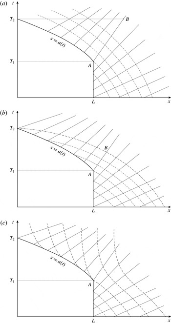It means that the $s$ -characteristics in problem (4.1)–(4.3) disperse in time (figure 2). Therefore, the solution of this problem is continuous and represents an $s$ -depression wave of the initial liquid of depth $h_{0}=1$ .

Figure 2.

Fields of characteristics in the cases $G=0$ (a), $G>0$ (b) and $G<0$ (c) at the first and second stages: the solid straight lines show the $s$ -characteristics; the dashed lines show the $r$ -characteristics.

5 Lifting of the beam with a finite initial velocity

In solving problem (4.1)–(4.3), in the case with $H^{\prime }(0)>0$ , the depth of the liquid adjacent to the beam at the point $x=L=1$ instantaneously (i.e. at the time $t=0$ ) decreases to a certain value $h_{L}(0)<1$ . In this case, for the inequality $T_{1}>0$ , the following condition should be valid:

(5.1) $$\begin{eqnarray}\displaystyle H(0)=h_{1}<h_{L}(0). & & \displaystyle\end{eqnarray}$$

Violation of this condition means that (within the shallow water theory) the depth of the liquid adjacent to the beam at the point $x=L+0$ is smaller than or equal to the depth of the liquid under the beam immediately after the beginning of beam lifting. As a result, the first stage of the flow considered in this work will be absent.

If the initial depth of the liquid under the beam is $h_{1}<h_{c}$ , condition (5.1) is satisfied by virtue of inequality (4.8). If the initial depth is $h_{1}\geqslant h_{c}$ , condition (5.1) leads to an additional constraint on the initial velocity of beam lifting

(5.2) $$\begin{eqnarray}\displaystyle H^{\prime }(0)<2h_{1}\left(1-\sqrt{h_{1}}\right). & & \displaystyle\end{eqnarray}$$

As the liquid depth $H(t)$ under the beam at the first stage continuously and strongly monotonically increases, while the depth $h_{L}(t)$ of the liquid adjacent to the beam continuously and monotonically decreases, for the considered problem to be well posed in the case with $h_{1}\geqslant h_{c}$ , it is sufficient to satisfy the condition (5.2) at the initial time, which means that the first stage of the flow exists; in the case with $h_{1}<h_{c}$ , it is sufficient to satisfy the condition (4.7) in the time interval $(0,T_{c})$ , where $H(T_{c})=h_{c}$ and $T_{c}\leqslant T_{1}$ . If the condition (4.7) is violated in the time interval $(0,T_{c})$ , such flows are not considered in this paper.

If the beam lifting velocity $H^{\prime }$ is constant and satisfies well-posedness condition (4.7) at $h_{1}\leqslant h_{c}$ or condition (5.2) of the first stage existence at $h_{1}\geqslant h_{c}$ , then the flow in the domain $x>1$ at the first stage is a centred $s$ -depression wave (Stocker Reference Stocker1957). In this case, the final time instant of the first stage is $T_{1}=(h_{L}-h_{1})/H^{\prime }$ .

For the description of wave flows at the second stage, first of all, it is necessary to define the law of motion of the boundary line $x=a(t)$ of the beam–liquid contact region. We will study various cases of such motion assuming that solutions of the considered problem are continuous on the boundary line.

6 Motion of the boundary line along the characteristic of the shallow water equations

Let us assume that beam lifting occurs under condition (3.9) at the second stage. Double integration of the second equation of this condition with initial data $H(T_{1})=H_{1}$ and $H^{\prime }(T_{1})=H_{1}^{\prime }$ yields

(6.1a,b ) $$\begin{eqnarray}\displaystyle H^{\prime }(t)=\frac{H_{1}^{\prime }H^{2}(t)}{H_{1}^{2}},\quad H(t)=\frac{H_{1}^{2}}{H_{1}-H_{1}^{\prime }(t-T_{1})},\quad t\in (T_{1},T_{2}),T_{2}<T_{1}+\frac{H_{1}}{H_{1}^{\prime }}.\qquad & & \displaystyle\end{eqnarray}$$

Substituting (6.1) into formula (3.2), we obtain the liquid velocity in such a flow:

(6.2) $$\begin{eqnarray}\displaystyle u(x,t)=-\frac{xH^{\prime }(t)}{H(t)}=-\frac{xH_{1}^{\prime }}{H_{1}-H_{1}^{\prime }(t-T_{1})}. & & \displaystyle\end{eqnarray}$$

The depth $h=H(t)$ defined by the second formula of (6.1) and the velocity $u$ defined by formula (6.2) represent the exact solution of the homogeneous system (4.1) defined in an infinite strip

(6.3a,b ) $$\begin{eqnarray}\displaystyle |x|<+\infty ,\quad t\in (T_{1},T_{2}),\quad T_{2}=T_{1}+H_{1}/H_{1}^{\prime }. & & \displaystyle\end{eqnarray}$$

This solution describes the process of filling of the entire space by the liquid at the final time $\unicode[STIX]{x0394}t=1/H_{1}^{\prime }$ owing to the inflow of the liquid from infinity.

In the considered simplest case, the beam at the second stage does not influence the flow of the liquid lifting behind it. At the beginning of the second stage, the temporal derivative of the flow depth has a discontinuity on the beam boundary $L=1$ :

(6.4) $$\begin{eqnarray}\displaystyle h_{t}(L+0,T_{1})=h_{L}^{\prime }(T_{1})\leqslant 0<h_{t}(L-0,T_{1})=H^{\prime }(T_{1}). & & \displaystyle\end{eqnarray}$$

This weak discontinuity of the exact solution lying on the boundary line $x=a(t)$ propagates along the $r$ -characteristic of the homogeneous system (4.1) with the velocity

(6.5) $$\begin{eqnarray}\displaystyle a^{\prime }=\unicode[STIX]{x1D706}_{r}=U-C=-aR-C,\quad C=\sqrt{H}. & & \displaystyle\end{eqnarray}$$

It follows from formula (6.5) that, for obtaining the function $x=a(t)$ , it is sufficient to integrate the ordinary differential equation

(6.6) $$\begin{eqnarray}\displaystyle a^{\prime }+aR+C=0 & & \displaystyle\end{eqnarray}$$

with the initial condition $a(T_{1})=L$ . In this case, however, it is more convenient to find the boundary line $x=a(t)$ by using the initial $r$ -invariant value

(6.7) $$\begin{eqnarray}\displaystyle r=U-2C=-aR-2C=r_{0}=-2, & & \displaystyle\end{eqnarray}$$

brought to the point $(L,T_{1})$ from the undisturbed part of the liquid.

From (6.7), taking into account formula (3.2) we obtain

(6.8) $$\begin{eqnarray}\displaystyle a(t)=\frac{2(1-C)}{R}=\frac{2H\left(1-\sqrt{H}\right)}{H^{\prime }}. & & \displaystyle\end{eqnarray}$$

Differentiating equation (6.8) and taking into account formulas (3.3) and (3.5), we obtain

(6.9) $$\begin{eqnarray}\displaystyle a^{\prime }=-\frac{2(1-C)R^{\prime }+2C^{\prime }R}{R^{2}}=-\frac{aR^{\prime }+2C^{\prime }}{R}=\frac{aG}{R}+U-C. & & \displaystyle\end{eqnarray}$$

From here, taking into account conditions (3.9), we find the sought velocity of boundary line propagation (6.5). It follows from (6.8) that separation of the beam from the liquid occurs at the origin of the coordinate system  $x=0$ , at the zero length of the contact region $a(T_{2})=0$ , at the depth

(6.10) $$\begin{eqnarray}\displaystyle h(0,T_{2})=H(T_{2})=1. & & \displaystyle\end{eqnarray}$$

After determining the position of the boundary line by (6.8), the flow in the external domain $x>a(t)$ is found by solving the initial boundary value problem for the system (4.1), with the initial data formed at $t=T_{1}$ and the boundary condition

(6.11) $$\begin{eqnarray}\displaystyle h(a(t),t)=H(t), & & \displaystyle\end{eqnarray}$$

defined on the moving boundary $x=a(t)$ . In the considered case, the liquid flow at the second stage can be also found by solving the initial boundary value problem for system (4.1) in the domain $x>0$ with the no-penetration boundary condition

(6.12) $$\begin{eqnarray}\displaystyle u(0,t)=q(0,t)=0. & & \displaystyle\end{eqnarray}$$

In such a calculation, the boundary line $x=a(t)$ is not allocated specially and is localized by the through computation.

Appendix A shows that the solution constructed in this section satisfies the correctness condition

(6.13) $$\begin{eqnarray}\displaystyle h(x,t)<H(t)\quad \forall \,x\in (a(t),1)\;\forall \,t\in (T_{1},T_{2}) & & \displaystyle\end{eqnarray}$$

of the considered problem.

7 Results of numerical simulations at $G=0$

In view of the symmetry of the problem with respect to the origin $x=0$ , the numerical solution of the homogeneous system of the shallow water equations (4.1) is performed in the domain $[1,4]$ at the first stage, in the domain $[a(t),4]$ with a moving left boundary at the second stage and in the domain $[0,4]$ at the third stage. The right boundary of the computational domain at $x=4$ is subjected to the non-reflecting boundary condition

(7.1) $$\begin{eqnarray}\displaystyle u(4,t)-2\sqrt{h(4,t)}=r_{0}=-2, & & \displaystyle\end{eqnarray}$$

which means preservation of the $r$ -invariant value brought from the undisturbed part $x>1+t$ of the liquid. The boundary condition (7.1) allows approximate modelling of the solution of an initial boundary value problem in a semi-infinite spatial interval.

The conditions imposed on the left boundaries of the computational domains are condition (4.3) at the first stage and the no-penetration condition

(7.2) $$\begin{eqnarray}\displaystyle u(0,t)=q(0,t)=0 & & \displaystyle\end{eqnarray}$$

at the third stage. The conditions on the moving left boundary $x=a(t)$ at the second stage depend on the propagation velocity of this boundary line. In the considered case, when the boundary line $x=a(t)$ propagates along the $r$ -characteristic of the shallow water system (4.1), only condition (6.11) is imposed on this line.

Figure 3.

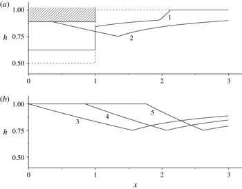
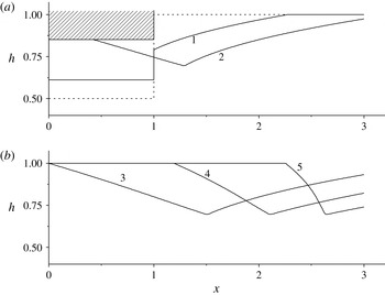
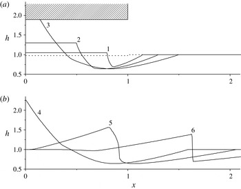
Wave profiles for five consecutive time instants for the case of beam lifting according to formula (7.3) with the initial velocity $H^{\prime }(0)=0.088$ at the initial depth of the liquid under the beam $h_{1}=0.5$ ; $t=1.131$ (1), 2.475 (2), 2.828 (3), 3.677 (4) and 4.596 (5).

For the numerical solution of system (4.1), we used the explicit second-order CABARET scheme (Goloviznin Reference Goloviznin2005). The main advantages of this scheme are provided by the following property: in the linear case, this scheme is reversible in time and exact for two different Courant numbers $r=0.5$ and $r=1$ . For this reason, the scheme possesses unique dissipative and dispersive properties (Karabasov & Goloviznin Reference Karabasov and Goloviznin2009). In view of the special flux correction the CABARET scheme is monotonic (Ostapenko Reference Ostapenko2012) at Courant numbers $r\leqslant 0.5$ . Therefore, the value $r=0.5$ is used in the computations described below. Moreover, the CABARET scheme has a compact stencil bounded by the size of one spatio-temporal cell of the difference grid. As a result, its accuracy does not decrease on severely non-uniform difference grids, which were used to construct the numerical algorithm at the second stage of the flow in the neighbourhood of the moving boundary $x=a(t)$ of the computational domain.

In all calculations described further, the beam is lifting in such a manner that condition (4.7) is satisfied at the first stage, which guarantees the correctness of problem (4.1)–(4.3). The dashed curves in the figures show the initial position of the liquid surface at $t=0$ . Let us assume that condition (3.9) holds during the first and second stages. In this case, it follows from (6.1) that the beam lifts by the law

(7.3) $$\begin{eqnarray}\displaystyle h(t)=H(t)=\frac{h_{1}^{2}}{h_{1}-tH^{\prime }(0)}. & & \displaystyle\end{eqnarray}$$

Figure 3 shows five consecutive instants of the results of numerical simulations of the considered problem for the case of beam lifting in accordance with law (7.3) for the initial velocity $H^{\prime }(0)=0.088$ and the initial depth of the liquid under the beam $h_{1}=0.5$ . At the second stage, the calculations were carried out in two ways. In the first case, system (4.1) is solved in the domain $[a(t),4]$ with a moving left boundary defined by formula (6.8); condition (6.11) is imposed on this boundary. In the second case, taking into account that the beam does not influence the liquid flow at $G=0$ at the second stage, we solve system (4.1) in the domain $[0,4]$ with the left boundary condition (7.2). The calculations performed on a sequence of consecutively refined grids show that the difference solutions obtained in these two ways converge to the same exact solution become visually indiscernible on a sufficiently fine grid. It is indirect confirmation of the correctness of formula (6.8) at  $G=0$ .

The results of numerical simulations show that the first stage of the considered problem, when the lower surface of the beam is completely immersed in water and the depression wave propagates in the domain $x>1$ (curve 1 in figure 3 a), is finalized at the time $T_{1}=1.9$ . The second stage, when the edges of the lower surface of the beam start to go out from the water (curve 2 in figure 3 a), is finalized at the time $T_{2}=2.83$ , when the beam separates from the liquid (curve 3 in figure 3 b). At $t>T_{2}$ , liquid lifting that occurred at the second stage leads to the formation of a wave of the liquid level increase (curves 4 and 5 in figure 3 b) propagating in the positive direction of the $x$ axis.

8 Motion of the boundary line with a subcritical velocity

Let us assume that the boundary line $x=a(t)$ in the second stage propagates with a subcritical velocity

(8.1) $$\begin{eqnarray}\displaystyle \unicode[STIX]{x1D706}_{s}=U+C>a^{\prime }>\unicode[STIX]{x1D706}_{r}=U-C & & \displaystyle\end{eqnarray}$$

and the exact solution of the considered problem is continuous in the curvilinear triangle $\widetilde{\unicode[STIX]{x1D6E5}}=ABT_{2}$ (figure 2 b) bounded by the boundary line $x=a(t)$ , the $s$ -characteristic leaving the point $A_{1}=(1,T_{1})$ and the $r$ -characteristic coming to the point $T_{2}$ on the $t$ axis. In this case, the $r$ -characteristics arriving on the boundary line $x=a(t)$ bring the initial value of the $r$ -invariant from the undisturbed part of the liquid. As a result, (6.7) yields explicit formulas for the boundary line (6.8) and for the velocity of its propagation (6.9).

In view of (3.3), (3.5), (6.8) and (6.9), inequalities (8.1) can be rewritten as

(8.2) $$\begin{eqnarray}\displaystyle 2CR>aG>0, & & \displaystyle\end{eqnarray}$$

where the first inequality can be presented in the form

(8.3) $$\begin{eqnarray}\displaystyle C(H^{\prime })^{2}>(1-C)(2(H^{\prime })^{2}-HH^{\prime \prime }). & & \displaystyle\end{eqnarray}$$

Since in the considered case $H^{\prime }>0$ , $H^{\prime \prime }\geqslant 0$ and $C=\sqrt{H}\leqslant 1$ , inequality (8.3) is satisfied under the condition $H>4/9$ , which, in view of (4.8), follows from the constraint $H>h_{L}(T_{1})\geqslant h_{c}=4/9$ . Thus, conditions (3.8) and (8.1) are equivalent at the second stage if the considered solution is continuous in the domain $\widetilde{\unicode[STIX]{x1D6E5}}$ .

If the liquid velocity $U$ on the boundary line $x=a(t)$ is greater than the line propagation velocity (6.9), i.e. if condition (8.1) is taken into account, the velocity $U$ satisfies the inequalities

(8.4) $$\begin{eqnarray}\displaystyle U>a^{\prime }=-\frac{aR^{\prime }+2C^{\prime }}{R}>U-C, & & \displaystyle\end{eqnarray}$$

the liquid outflows from the domain $|x|\leqslant a(t)$ adjacent to the beam. Taking into account (3.3), (3.5) and (6.8), we can present the first inequality of (8.4) in the form

(8.5) $$\begin{eqnarray}\displaystyle 2(1-C)HH^{\prime \prime }>(4-5C)(H^{\prime })^{2}. & & \displaystyle\end{eqnarray}$$

As $H^{\prime \prime }\geqslant 0$ and $C\leqslant 1$ inequality (8.5) is obviously satisfied under the condition $H=C^{2}>16/25$ . It follows from here that, if the liquid depth at the end of the first stage satisfies the condition $4/9<H(T_{1})<16/25$ and the inequality opposite to (8.5) is valid at $t=T_{1}$ , the liquid flows into the domain $|x|\leqslant a(t)$ at the beginning of the second stage.

It follows from (6.8) that, as in the case with $G=0$ , separation of the beam from the liquid occurs at depth (6.10), and at the time instant $T_{2}=H^{-1}(1)$ , where $H^{-1}(h)$ is a function inverse to $H(t)$ . In particular, if the beam lifts with a constant velocity during the first and second stages, we have

(8.6) $$\begin{eqnarray}\displaystyle T_{2}=\frac{1-h_{1}}{H^{\prime }(0)}. & & \displaystyle\end{eqnarray}$$

As inequality (8.5) is satisfied in some time interval $(t_{2},T_{2})$ , where $t_{2}\geqslant T_{1}$ , the liquid always outflows from the domain $|x|\leqslant a(t)$ at the end of the second stage.

Figure 4.

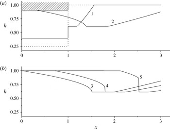
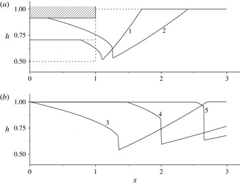
Wave profiles for five consecutive time instants for the case of beam lifting with the constant velocity $H^{\prime }(0)=0.265$ at the initial depth of the liquid under the beam $h_{1}=0.25$ ; $t=0.566$ (1), 2.475 (2), 2.828 (3), 3.536 (4) and 4.950 (5).

After determining the position of the boundary line by (6.8), the flow in the external domain $x>a(t)$ under condition (3.8) is found by solving the initial boundary value problem for the system (4.1) with the initial data formed at $t=T_{1}$ and the boundary condition (6.11). In the considered case with $G>0$ , in contrast to the case with $G=0$ , the validity of correctness conditions (6.13) on the entire segment $[a(t),1]$ is verified by means of numerical calculations. At the same time, with taking into account that the solution

(8.7a,b ) $$\begin{eqnarray}\displaystyle h(a(t),t)=H(t),\quad u(a(t),t)=U(t) & & \displaystyle\end{eqnarray}$$

is known on the boundary line $x=a(t)$ , the condition (6.13) can be verified analytically in a certain neighbourhood of the boundary line (see appendix B).

9 Results of numerical simulations at $G>0$

Figures 4–6 show the results of numerical simulations of the considered problem for the case of beam lifting in such a manner that condition (3.8) is satisfied and the exact solution is continuous in the domain $\widetilde{\unicode[STIX]{x1D6E5}}$ , which guarantees the well posedness of formula (6.8) for the boundary line $x=a(t)$ propagating with the subcritical velocity (8.1) defined by (6.9). At the second stage, system (4.1) is solved in the domain $[a(t),4]$ in two ways. In the first case, the left moving boundary of this domain is defined by formula (6.8), and condition (6.11) is imposed on this boundary. In the second case, two boundary conditions (8.7) are imposed on the boundary line $x=a(t)$ ; the position of this line is not defined by an exact formula; it is calculated in the course of solving system (4.1) in the domain $[a(t),4]$ . The calculations performed on a sequence of gradually refined grids show that the difference solutions obtained in these two ways converge to the same exact solution and become visually indiscernible on a sufficiently fine grid. It is indirect confirmation of the correctness of formula (6.8) for numerical simulations illustrated in figures 4–6.

Figure 5.

Wave profiles for five consecutive time instants for the case of beam lifting with the constant acceleration $H^{\prime \prime }(0)=0.138$ at the initial depth of the liquid under the beam $h_{1}=0.5$ ; $t=1.273$ (1), 2.263 (2), 2.701 (3), 3.889 (4) and 4.950 (5).

Figure 6.

Wave profiles for five consecutive time instants for the case of beam lifting with the constant acceleration $H^{\prime \prime }(0)=0.293$ at the initial depth of the liquid under the beam $h_{1}=0.5$ ; $t=0.707$ (1), 1.414 (2), 1.711 (3), 3.182 (4) and 4.243 (5).

In figure 4, the beam is lifting with a constant velocity $H^{\prime }(0)=0.265$ at the initial depth of the liquid under the beam $h_{1}=1/4$ , which, by virtue of condition (4.7) and the inequality $h_{1}<4/9$ , ensures the existence of the first stage of the flow. This stage, when the lower surface of the beam is completely immersed in water and the centred depression waves propagate in the domain $x>1$ (curve 1 in figure 4 a), is finalized at the time $T_{1}=1.38$ . The second stage, when the edges of the lower surface of the beam start to go out from the water (curve 2 in figure 4 a), is finalized, as predicted by formula (8.6), at the time $T_{2}=2.83$ when the beam separates from the liquid (curve 3 in figure 4 b). At $t>T_{2}$ , liquid lifting that occurred at the second stage leads to the formation of a shock wave moving in the positive direction of the $x$ axis (curves 4 and 5 in figure 4 b).

In figure 5, the beam is lifting with a constant acceleration $H_{0}^{\prime \prime }=0.138$ and zero initial velocity (which guarantees the existence of the first stage of the flow) at the initial depth $h_{1}=1/2$ . The first stage, when the lower surface of the beam is completely immersed in water (curve 1 in figure 5 a), is finalized at the time $T_{1}=1.68$  s, and the second stage shown by curve 2 in figure 5(a) is finalized at the time $T_{2}=2.70$  s (curve 3 in figure 5 b). At $t>T_{2}$ , liquid lifting that occurred at the second stage leads to the formation of a wave of the liquid level increase (curves 4 and 5 in figure 5 b).

In figure 6, the beam is lifting from the initial depth $h_{1}=1/2$ with a constant velocity

(9.1) $$\begin{eqnarray}\displaystyle H^{\prime }(0)=2h_{1}\left(1-\sqrt{h_{1}}\right)=1-1/\sqrt{2}\approx 0.293, & & \displaystyle\end{eqnarray}$$

which leads to violation of condition (5.2) necessary for the existence of the first stage of the flow. As a result, the second stage shown by curves 1 and 2 in figure 6(a) begins immediately after the beginning of beam lifting and ends at the time $T_{2}=1.71$ (curve 3 in figure 6 b). At the third stage ( $t>T_{2}$ ), liquid lifting that occurs at the second stage leads to the formation of a shock wave moving in the positive direction of the $x$ axis (curves 4 and 5 in figure 6 b). Let us note that in figures 4(b) and 6(b) the strong discontinuities are the shock waves (Friedrichs & Lax Reference Friedrichs and Lax1971; Lax Reference Lax1972) modelling the hydraulic bores of the real flow.

10 Energy conservation law in the domain adjacent to the beam

Let us assume that beam lifting in some time interval $(t_{1},t_{2})\subseteq (T_{1},T_{2})$ at the second stage occurs under condition (3.10). In this case, it follows from formulas (B 5)–(B 7) that the local correctness condition

(10.1) $$\begin{eqnarray}\displaystyle h_{x}^{+}(t)=\frac{\unicode[STIX]{x1D6E5}_{1}}{\unicode[STIX]{x1D6E5}}=\frac{aHG}{(a^{\prime }-\unicode[STIX]{x1D706}_{r})(a^{\prime }-\unicode[STIX]{x1D706}_{s})}<0\quad \forall \,t\in (t_{1},t_{2}) & & \displaystyle\end{eqnarray}$$

implies propagation of the boundary line $x=a(t)$ with a supercritical velocity

(10.2) $$\begin{eqnarray}\displaystyle a^{\prime }<\unicode[STIX]{x1D706}_{r}=U-C<\unicode[STIX]{x1D706}_{s}=U+C & & \displaystyle\end{eqnarray}$$

and does not imply its propagation with the subcritical velocity (8.1). If the boundary line propagates with the supercritical velocity (10.2), then the $r$ - and $s$ -characteristics of system (4.1) emanate from this line in the domain $x>a(t)$ , and none of them arrive on the line $x=a(t)$ (figure 2 c). This means that the external flow at $x>a(t)$ does not affect the boundary line motion within the framework of the shallow water theory. As a result, for definition of the boundary line position from (3.3) at $G<0$ , it is necessary to use one more additional relation, which should be derived from the fundamental physical law of the liquid flow in the domain $|x|\leqslant a(t)$ adjacent to the beam.

Therefore, we consider the energy conservation law in the two-dimensional spatial domain

(10.3) $$\begin{eqnarray}\displaystyle S(t)=\{(x,z):|x|\leqslant a(t),0\leqslant z\leqslant H(t)\}. & & \displaystyle\end{eqnarray}$$

The conservation law will be written in dimensionless variables (2.3)–(2.5) in which the asterisk is omitted for the brevity. Within the long-wave approximation (2.1), (2.2), the total energy $E$ of the liquid in this domain, which is the sum of the kinetic and potential energies, in view of (3.2) and (3.3) is determined by the formula

(10.4) $$\begin{eqnarray}\displaystyle E=\int _{-a}^{a}\left(\int _{0}^{H}\left(\frac{u^{2}}{2}+z\right)\text{d}z\right)\text{d}x=aH\left(\frac{U^{2}}{3}+H\right). & & \displaystyle\end{eqnarray}$$

The change in the total energy (10.4) results from its flux with the velocity

(10.5) $$\begin{eqnarray}\displaystyle V_{E}=2(U-a^{\prime })\int _{0}^{H}\left(\frac{U^{2}}{2}+z\right)\text{d}z=H(U-a^{\prime })\left(U^{2}+H\right) & & \displaystyle\end{eqnarray}$$

through the moving lateral boundaries $x=\pm a(t)$ of domain (10.3) and from the pressure work

(10.6) $$\begin{eqnarray}\displaystyle W_{1}=-2a^{\prime }\int _{0}^{H}p(a,z,t)\,\text{d}z=-2a^{\prime }\int _{0}^{H}(H-z)\,\text{d}z=-a^{\prime }H^{2}, & & \displaystyle\end{eqnarray}$$

on these lateral boundaries, where $p(x,z,t)=H(t)-z$ is the hydrostatic law of pressure. The change in the total energy (10.4) occurs also results from the pressure work $W_{2}=-PH^{\prime }$ on the top moving boundary $z=H(t)$ of domain (10.3). The total pressure force $P$ is calculated by the formula

(10.7) $$\begin{eqnarray}\displaystyle P(t)=\int _{-a(t)}^{a(t)}\widetilde{p}(x,t)\,\text{d}x=\frac{2a^{3}(t)G(t)}{3}, & & \displaystyle\end{eqnarray}$$

where the surface pressure $\widetilde{p}(x,t)$ is determined by (3.7). As a result, we have

(10.8) $$\begin{eqnarray}\displaystyle W_{2}=-PH^{\prime }=-\frac{2a^{3}GH^{\prime }}{3}=\frac{2a^{3}(R^{\prime }-R^{2})H^{\prime }}{3}. & & \displaystyle\end{eqnarray}$$

Part of the total energy (10.4) transforms with some speed $\unicode[STIX]{x0394}E$ to the energy of liquid vortices concentrated in small areas $|x\pm a(t)|<\unicode[STIX]{x1D6FF}$ of the boundary lines $x=\pm a(t)$ whose sizes $2\unicode[STIX]{x1D6FF}$ are neglected within the long-wave approximation. Since the shallow water equations (4.1) represent the hyperbolic system of conservation laws with convex expansion (Friedrichs & Lax Reference Friedrichs and Lax1971; Lax Reference Lax1972), an energy transition $\unicode[STIX]{x0394}E$ is similar to the losses of the total energy to shock waves in the classical shallow water theory (Stocker Reference Stocker1957; Ostapenko Reference Ostapenko2007; Chaudhry Reference Chaudhry2008). Taking this into consideration, we obtain the total energy conservation law in domain (10.3) from (10.4)–(10.8):

(10.9) $$\begin{eqnarray}\displaystyle \frac{\text{d}E}{\text{d}t}+V_{E}+\unicode[STIX]{x0394}E=W_{1}+W_{2}. & & \displaystyle\end{eqnarray}$$

After conversions, (10.9) can be written in the form

(10.10) $$\begin{eqnarray}\displaystyle \unicode[STIX]{x0394}E=H^{2}(U-a^{\prime }), & & \displaystyle\end{eqnarray}$$

which will be used for obtaining an additional relation that allows one to determine the velocity of the boundary line $x=a(t)$ under condition (3.10).

11 Motion of the boundary line under the condition $G<0$

As the basic criterion that allows one to determine the position of the boundary line $x=a(t)$ under condition (3.10), we use the assumption that the minimum possible part of the total energy of the liquid transforms to the vortex energy $\unicode[STIX]{x0394}E$ when the liquid leaves domain (10.3). As a result we have from (10.10) under constraint (10.2) that the liquid flow occurs under the condition

(11.1) $$\begin{eqnarray}\displaystyle \unicode[STIX]{x0394}E=\inf _{a^{\prime }<\unicode[STIX]{x1D706}_{r}}H^{2}(U-a^{\prime })=H^{2}C=H^{5/2}. & & \displaystyle\end{eqnarray}$$

Hence the boundary line $x=a(t)$ propagates with the critical velocity (6.5). The acceleration of such propagation, taking into account (3.3), (3.5) and (6.5), is calculated by the formula

(11.2) $$\begin{eqnarray}\displaystyle a^{\prime \prime }=(U-C)^{\prime }=-(aR)^{\prime }-C^{\prime }=a(R^{2}-R^{\prime })+RC-C^{\prime }=aG+C^{\prime }. & & \displaystyle\end{eqnarray}$$

If the point $(a(t),t)$ of the boundary line $x=a(t)$ lies on the $r$ -characteristic of system (4.1), where the $r$ -invariant has a constant value $r_{1}$ , the liquid and sound velocities $U=U(a(t),t)$ and $C=C(a(t),t)$ at this point satisfy the condition $U=2C+r_{1}$ , whereas the $r$ -characteristic velocity at this point is calculated by the formula $\unicode[STIX]{x1D706}_{r}=U-C=C+r_{1}.$ From here, the $r$ -characteristic acceleration on the boundary line is

(11.3) $$\begin{eqnarray}\displaystyle \unicode[STIX]{x1D706}_{r}^{\prime }=(C+r_{1})^{\prime }=C^{\prime }. & & \displaystyle\end{eqnarray}$$

It follows from (11.2) and (11.3) that the boundary line propagating with the $r$ -critical velocity at $G<0$ is the envelope of the $r$ -characteristics emanating from this line in the external domain $x>a(t)$ (figure 2 c). This means that the flow in the domain $x>a(t)$ does not affect the liquid flow in the domain $|x|\leqslant a(t)$ adjacent to the beam. Formula (6.5) yields the ordinary differential equation (6.6) for the boundary line $x=a(t)$ . Integrating this equation in the time interval $(t_{1},t_{2})$ , we obtain

(11.4) $$\begin{eqnarray}\displaystyle a(t)=\frac{1}{H(t)}\left(a(t_{1})H(t_{1})-\int _{t_{1}}^{t}H^{3/2}(\unicode[STIX]{x1D703})\,\text{d}\unicode[STIX]{x1D703}\right),\quad t\in (t_{1},t_{2}). & & \displaystyle\end{eqnarray}$$

It follows from inequalities (10.1) and (10.2) that

(11.5) $$\begin{eqnarray}\displaystyle \lim _{a^{\prime }\rightarrow \unicode[STIX]{x1D706}_{r}-0}h_{x}^{+}(t)=-\infty . & & \displaystyle\end{eqnarray}$$

Which means that, in the case of the boundary line (11.4) propagating with the critical velocity (6.5), the free liquid surface comes up to the bottom beam surface at a right angle within the long-wave approximation.

12 Results of numerical simulations at $G<0$ at the beginning of the second stage

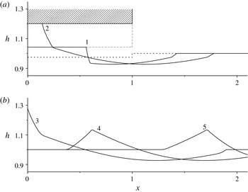
Figures 7–9 show the results of numerical simulations of the considered problem for the case of beam lifting with a constant acceleration and zero initial velocity in such a manner that condition (3.10) is satisfied at the beginning of the second stage. In figure 7, the beam lifts with the acceleration $H^{\prime \prime }=0.75$ from the initial depth $h_{1}=0.975$ , which can be approximately interpreted as the beam lifting from the surface of the undisturbed liquid. In this case, inequality $G<0$ is satisfied during the entire second stage (curves 1 and 2 in figure 7 a), which ends at the time instant $T_{2}=0.905$ , when the maximum liquid lifting $h(0,T_{2})=1.28$ is reached (curve 3 in figure 7 b).

Figure 7.

Wave profiles for five consecutive time instants for the case of beam lifting with the constant acceleration $H_{0}^{\prime \prime }=0.75$ and zero initial velocity at the initial depth of the liquid under the beam $h_{1}=0.975$ ; $t=0.424$ (1), 0.778 (2), 0.905 (3), 1.414 (4) and 2.333 (5).

Figure 8.

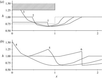
Wave profiles for six consecutive time instants for the case of beam lifting with the constant acceleration $H_{0}^{\prime \prime }=2.5$ and zero initial velocity at the initial depth of the liquid under the beam $h_{1}=0.75$ ; $t=0.212$ (1), 0.453 (2), 0.636 (3), 0.792 (4), 1.414 (5) and 2.121 (6).

Figure 9.

Wave profiles for six consecutive time instants for the case of beam lifting with the constant acceleration $H_{0}^{\prime \prime }=7.5$ and zero initial velocity at the initial depth of the liquid under the beam $h_{1}=0.975$ ; $t=0.141$ (1), 0.294 (2), 0.495 (3), 0.587 (4), 1.061 (5) and 1.697 (6).

In figure 8, the beam lifts with acceleration $H^{\prime \prime }=2.5$ from the initial depth $h_{1}=0.75$ . In this case, inequality $G<0$ is satisfied only at the beginning of the second stage (curve 1 in figure 8 a) in the time interval $(T_{1},t_{2})\subseteq (T_{1},T_{2})$ , where $T_{1}=0.085$ , $t_{2}=0.453$ , $a(t_{2})=0.468$ and $T_{2}=0.792$ . At the time instant  $t_{2}$ (curve 2 in figure 8 a), the function $G$ changes its sign, and beam lifting in the time interval $(t_{2},T_{2})$ occurs under the inequality $G>0$ (curve 3 in figure 8 a). At the end of the second stage (curve 4 in figure 8 b), the maximum liquid lifting $h(0,T_{2})=1.53$ is reached.

In figure 9, the beam lifts with the acceleration $H^{\prime \prime }=7.5$ from the initial depth $h_{1}=0.975$ . In this case, inequality $G<0$ is satisfied only at the beginning of the second stage (curve 1 in figure 9 a) in the time interval $(T_{1},t_{2})\subseteq (T_{1},T_{2})$ , where $T_{1}=0.003$ , $t_{2}=0.294$ , $a(t_{2})=0.497$ and $T_{2}=0.587$ . At the time instant  $t_{2}$ (curve 2 in figure 9 a), the function $G$ changes its sign, and beam lifting in the time interval $(t_{2},T_{2})$ occurs under the inequality $G>0$ (curve 3 in figure 9 a). At the end of the second stage (curve 4 in figure 9 b), the maximum liquid lifting $h(0,T_{2})=2.27$ is reached. Let us note that in figures 8(b) and 9(b) the strong discontinuities are the shock waves modelling the hydraulic bores of the real flow.

At the second stage, two boundary conditions (8.7) for system (4.1) are imposed on the left moving boundary of the computational domain $[a(t),4]$ . If inequality  $G<0$ is satisfied in the time interval $(T_{1},t_{2})\subseteq (T_{1},T_{2})$ , setting of the two boundary conditions on boundary line (11.4) is related to the fact that both characteristics pass from this line to the external domain $x>a(t)$ . If the inequality $G>0$ is satisfied in the time interval $(t_{2},T_{2})\subset (T_{1},T_{2})$ , in view that the inequality $G<0$ is satisfied in the previous time interval $(T_{1},t_{2})$ , the boundary line $x=a(t)$ at $t\in (t_{2},T_{2})$ is described by the equation $a(t)=-(2C+r_{1})/R$ derived from the formula $U-2C=-aR-2C=r_{1}$ , where $r_{1}$ is the $r$ -invariant value brought along the $r$ -characteristic coming from the domain $x>a(t)$ to the boundary line. Thus, the line can propagate both with the $r$ -critical (6.5) and subcritical (8.1) velocities. It follows from formulas (11.2) and (11.3) that the boundary line $x=a(t)$ in the first case is the envelope of the $r$ -characteristics coming to this line from the external domain $x>a(t)$ . Unlike the situation studied in §§ 8 and 9, the $r$ -invariant value $r_{1}$ in the considered case is unknown in advance. Therefore the only way to solve the problem is where the two boundary conditions (8.7) are imposed on the boundary line $x=a(t)$ , and the position of this line is calculated in the course of solving system (4.1) in the domain $[a(t),4]$ .

The results of numerical calculations presented in figures 7–9 show that the maximum lifting of the liquid behind the beam can be appreciably greater than the initial liquid depth $h_{0}=1$ if condition (3.10) is satisfied at the beginning of the second stage. Thus, an increase in the acceleration of beam lifting leads to an increase in the maximum height of liquid lifting. The numerical calculations performed under the condition that the beam lifts with acceleration $H^{\prime \prime }>7.5$ show a further increasing of the maximum lifting of the liquid.