1. Introduction
We consider a continuous-time Galton–Watson (GW) process with branching rate
 $\beta>0$
and offspring distribution
 $(p_k)_{k \geq 0}$
initiated by a single particle. Such a process may be constructed as follows. It starts with a single particle at time 0. This initial particle lives for a random time T that is exponentially distributed with rate parameter
 $\beta$
. That is,
 $\mathbb{P}(T > t) = \mathrm{e}^{- \beta t}$
and
 $\mathbb{E} T = {1}/{\beta}$
. At the moment when the initial particle dies, it produces a random number
 $\xi$
of new particles where
 $\mathbb{P}(\xi = k) = p_k$
for every integer
 $k \geq 0$
. Newly born particles, independently of each other and of all the previous history, replicate the initial particle’s behaviour, that is, they live for random times with
 $\mathrm{Exp}(\beta)$
distribution, produce random numbers of new particles according to the offspring distribution
 $(p_k)_{k \geq 0}$
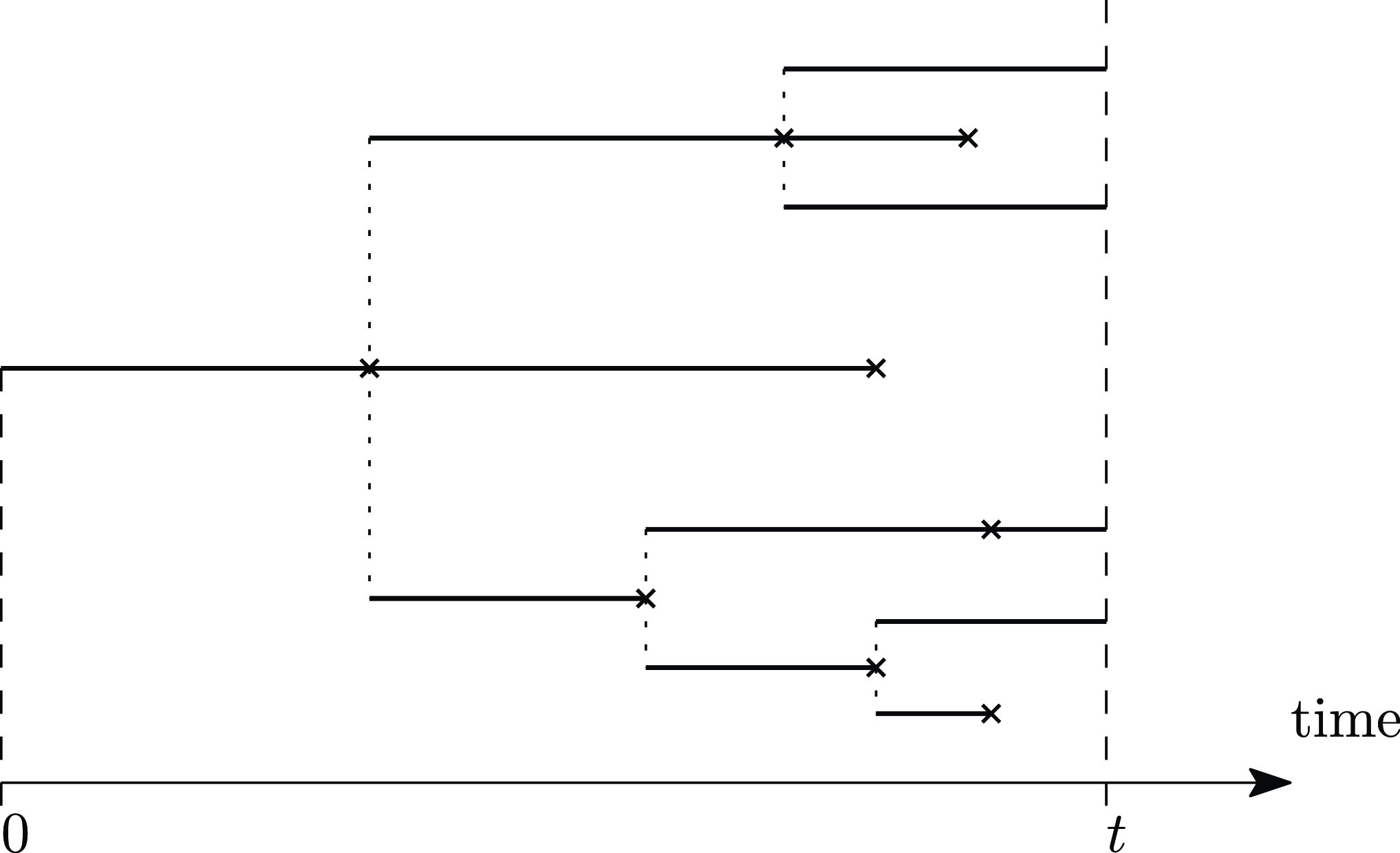
at the moment of their death, and so on. Graphically, such a process is most naturally represented by a tree in which each edge corresponds to the life span of a particle, as in Figure 1. We use
 $\mathcal{T}_t$
to denote the entire process (tree) evolved up to time t.
A typical realisation of
 $\mathcal{T}_t$
.

In this article we study the limiting behaviour of the longest edges in
 $\mathcal{T}_t$
as
 $t \to \infty$
. We classify edges in
 $\mathcal{T}_t$
as either pendant (edges corresponding to particles alive at time t) or interior (all other edges). If we think of
 $\mathcal{T}_t$
as describing some sort of evolutionary process then pendant edges would correspond to extant species and interior edges would correspond to extinct species.
Throughout, we assume the generic offspring random variable
 $\xi$
has mean
 $m:=\mathbb{E} \xi>1$
(the Galton–Watson process is supercritical and has some strictly positive chance of surviving forever), as well as the classical condition that
 $\mathbb{E} [\xi\log^+ \xi]<\infty$
. (Note, these assumptions permit cases where the offspring variance can be infinite.) Conditional on survival of the population, for any real number x, we will show that, for large times t, the number of pendant edges longer than
 $(1-1/m)t +x$
converges in distribution to a mixture of Poisson random variables with (random) parameter
 ${\mathrm{e}}^{-m\beta x}M_\infty$
, where the random variable
 $M_\infty$
is the classical additive martingale limit for the GW process. (Intuitively speaking,
 $M_\infty$
roughly measures the growth of the process during its earlier stages; alternatively,
 $\log M_\infty$
can be thought of as a random time delay for the process to get very large and start behaving deterministically.) As a corollary, we show that the length of the kth-longest pendant edge at large times t converges in distribution when centred around
 $(1-1/m)t$
, and we give an explicit representation for this limiting law. In particular, the length of the longest pendant edge at time t minus
 $(1-1/m)t$
converges in the large-time t limit to a mixture of Gumbel distributions.
Similarly, we prove analogous results for the longest interior edges and the longest of all edges. It turns out that long edges should always be centred around size
 $(1-1/m)t$
and always converge to a mixture of Poisson distributions, where only the mixture parameter varies according to whether long pendant, long interior, or longest of all edges are being considered. The analysis and proofs for the longest interior edges, and similarly longest of all edges, turn out to be more delicate and require considerably more involved calculations than the longest pendant edges case (where there is much more independence). The ‘
 $L\log L$
’ moment assumption is expected to be the best possible for our results to hold in light of the natural appearance of
 $M_\infty$
in the description of the limit and the classical Kesten–Stigum theorem for GW processes. However, as this assumption permits the offspring variance to be infinite in general, it necessitates an additional careful truncation argument to allow application of a second-moment method involving use of the Paley–Zygmund inequality.
Let us note that our methods, in principle, could be used to obtain similar results for maximal processes of other quantities in
 $\mathcal{T}_t$
, such as the maximal degree.
1.1. Preliminaries
We use m to denote the mean of the offspring distribution:
 $m := \mathbb{E} \xi = \sum_{k \geq 0} kp_k$
. As we shall see, this is the only quantity that determines the first-order limiting behaviour of all the longest edges in the tree. We also use v to denote the second moment of the offspring distribution:
 $v := \mathbb{E} \big[ \xi^2 \big] = \sum_{k \geq 0} k^2p_k$
. In this article it is always assumed that
 $m < \infty$
, whereas v may be finite or infinite.
We denote the number of particles alive at time t by
 $N_t$
, and the event of the population surviving forever by
 $\{ \text{survival} \} := \bigcap_{t \geq 0} \{N_t > 0\}$
. We let
 $\{$
extinction
 $\} = \{$
survival
 $\}^\mathrm{c}$
be the event of the population eventually becoming extinct.
It is well known that the process
 \begin{equation} M_t = \mathrm{e}^{-(m-1)\beta t} N_t, \quad t \geq 0,\end{equation}
is a (positive) martingale, which then has an almost-sure limit
 $M_\infty = \lim_{t \to \infty} M_t$
.
We make the following assumptions:
 \begin{align} m & > 1,\end{align}
 \begin{align} \mathbb{E}[\xi\log^+\xi] = \sum_{k \geq 1} k \log k \, p_k & < \infty.\\[5pt] \nonumber \end{align}
Condition (A1) is necessary and sufficient for
 $\mathbb{P}($
survival
 $) > 0$
and is known as the supercritical case. If condition (A1) is satisfied then the celebrated Kesten–Stigum theorem says that condition (A2) is necessary and sufficient for
 $\mathbb{P}(M_\infty > 0 \mid \mathrm{survival}) = 1$
or, in other words, for events
 $\{M_\infty > 0\}$
and
 $\{$
survival
 $\}$
to agree almost surely (see, e.g., [Reference Olofsson7]). This gives a fine approximation of the population growth:
 $N_t \sim M_\infty \mathrm{e}^{(m-1)\beta t}$
as
 $t \to \infty$
almost surely (a.s.) on survival (‘a.s. on survival’ is commonly used to mean ‘
 $\mathbb{P}(\,\cdot \mid \mathrm{survival}) = 1$
’). We remark that if condition (A2) is not satisfied then
 $\mathbb{P}(M_\infty=0 ) = 1$
and establishing the precise growth rate of
 $N_t$
is a difficult task.
1.2. Main results
We let
 $\alpha^\ast := 1 - {1}/{m}$
. As we shall soon see, all the longest edges in
 $\mathcal{T}_t$
are approximately of length
 $\alpha^\ast t$
for t large.
Definition 1. For a length
 $l \geq 0$
and a time
 $t \geq 0$
we define
 $N_t^l$
,
 $\hat{N}_t^l$
, and
 $\tilde{N}_t^l$
respectively to be the numbers of pendant, interior, and all (counting both pendant and interior) edges in
 $\mathcal{T}_t$
of length
 $\geq l$
. Note that in what follows we shall often take l to be dependent on t.
For all the results stated here we assume that conditions (A1) and (A2) hold. We let
 $\alpha^\ast$
be as just defined, and
 $M_\infty$
be the almost-sure limit of the martingale
 $M_t$
in (1).
Theorem 1.
Let
 $x \in \mathbb{R}$
be fixed,
 $t \geq 0$
variable, and
 $l = l(t) = \alpha^\ast t + x$
. Then, under
 $\mathbb{P}(\,\cdot \mid \mathrm{survival})$
,
 \begin{equation} N_t^l \Rightarrow V_x , \qquad \hat{N}_t^l \Rightarrow \hat{V}_x, \qquad \tilde{N}_t^l \Rightarrow \tilde{V}_x \end{equation}
as
 $t \to \infty$
, where
 $V_x$
,
 $\hat{V}_x$
, and
 $\tilde{V}_x$
are mixtures of Poisson distributions with respective rates
 $\mathrm{e}^{-m \beta x} M_\infty$
,
 $({1}/({m-1}))\mathrm{e}^{-m \beta x} M_\infty$
, and
 $({m}/({m-1}))\mathrm{e}^{-m \beta x} M_\infty$
conditional on
 $M_\infty >0$
. To be precise, for
 $k = 0,1,2,\ldots$
,
 \begin{align} \mathbb{P}(V_x = k \mid \mathrm{survival}) & = \mathbb{E}\bigg[\frac{1}{k!}\big(\mathrm{e}^{-m\beta x}M_\infty\big)^k \exp\big\{{-}\mathrm{e}^{-m\beta x}M_\infty\big\} \mid M_\infty > 0 \bigg], \nonumber \\ \mathbb{P}(\hat{V}_x = k \mid \mathrm{survival}) & = \mathbb{E}\bigg[\frac{1}{k!}\bigg(\frac{\mathrm{e}^{-m\beta x}M_\infty}{m-1}\bigg)^k \exp\bigg\{{-}\frac{\mathrm{e}^{-m\beta x}M_\infty}{m-1}\bigg\} \mid M_\infty > 0\bigg],\end{align}
 \begin{align} \mathbb{P}(\tilde{V}_x = k \mid \mathrm{survival}) & = \mathbb{E}\bigg[\frac{1}{k!}\bigg(\frac{m\mathrm{e}^{-m\beta x}M_\infty}{m-1}\bigg)^k \exp\bigg\{{-}\frac{m\mathrm{e}^{-m\beta x}M_\infty}{m-1}\bigg\} \mid M_\infty > 0\bigg]. \\[6pt]\nonumber \end{align}
In fact, if we let
 $l^k_t$
,
 $k=1,\ldots,N_t$
,
 $\hat{l}^k_t$
,
 $k=1,\ldots,\hat{N}_t$
, and
 $\tilde{l}^k_t$
,
 $k=1,\ldots,\tilde{N}_t$
be the lengths of pendant, interior, and all edges in
 $\mathcal{T}_t$
respectively then it can be shown that the point processes
 $\sum_{k=1}^{N_t} \delta_{l^k_t - \alpha^\ast t}$
,
 $\sum_{k=1}^{\hat{N}_t} \delta_{\hat{l}^k_t - \alpha^\ast t}$
, and
 $\sum_{k=1}^{\tilde{N}_t} \delta_{\tilde{l}^k_t - \alpha^\ast t}$
converge weakly to mixtures of Poisson point processes with intensities
 $M_\infty\mathrm{e}^{-m \beta x}\,\mathrm{d}x$
,
 $M_\infty({1}/({m-1}))\mathrm{e}^{-m\beta x}\,\mathrm{d}x$
, and
 $M_\infty({m}/({m-1}))\mathrm{e}^{-m\beta x}\,\mathrm{d}x$
, respectively. This, among other generalisations, will be established formally in a follow-up paper.
From Theorem 1 we can recover the limiting distributions of all longest edges in
 $\mathcal{T}_t$
(shifted by
 $\alpha^\ast t$
).
Definition 2. For
 $k = 1,2,3,\ldots$
let
 $L_t^{(k)}$
,
 $\hat{L}_t^{(k)}$
, and
 $\tilde{L}_t^{(k)}$
be the lengths of the kth longest edge among pendant, interior, and all edges in
 $\mathcal{T}_t$
respectively.
Corollary 1.
For all
 $k=1,2,3,\ldots$
, under
 $\mathbb{P}(\,\cdot \mid \mathrm{survival})$
,
 \begin{equation} L_t^{(k)} - \alpha^\ast t \Rightarrow W^{(k)}, \qquad \hat{L}_t^{(k)} - \alpha^\ast t \Rightarrow \hat{W}^{(k)}, \qquad \tilde{L}_t^{(k)} - \alpha^\ast t \Rightarrow \tilde{W}^{(k)}, \end{equation}
where
 \begin{align*} \mathbb{P}\big(W^{(k)} \leq x \mid \mathrm{survival}\big) & = \mathbb{E}\Bigg[\sum_{j=0}^{k-1}\frac{1}{j!}\big(\mathrm{e}^{-m\beta x}M_\infty\big)^j \exp\big\{{-}\mathrm{e}^{-m\beta x}M_\infty\big\} \mid M_\infty > 0\Bigg], \\ \mathbb{P}\big(\hat{W}^{(k)} \leq x \mid \mathrm{survival}\big) & = \mathbb{E}\Bigg[\sum_{j=0}^{k-1}\frac{1}{j!}\bigg(\frac{\mathrm{e}^{-m\beta x}M_\infty}{m-1}\bigg)^j \exp\bigg\{{-}\frac{\mathrm{e}^{-m\beta x}M_\infty}{m-1}\bigg\} \mid M_\infty > 0\Bigg], \\ \mathbb{P}\big(\tilde{W}^{(k)} \leq x \mid \mathrm{survival}\big) & = \mathbb{E}\Bigg[\sum_{j=0}^{k-1}\frac{1}{j!}\bigg(\frac{m\mathrm{e}^{-m\beta x}M_\infty}{m-1}\bigg)^j \exp\bigg\{{-}\frac{m\mathrm{e}^{-m\beta x}M_\infty}{m-1}\bigg\} \mid M_\infty > 0 \Bigg]. \end{align*}
In particular, the limiting distributions of the longest pendant, interior, and any edge centred around
 $\alpha^\ast t$
are mixtures of Gumbel distributions:
 \[ \mathbb{P}\big(W^{(1)} \leq x \mid \mathrm{survival}\big) = \mathbb{E}\big[\exp\big\{{-}\mathrm{e}^{-m\beta x}M_\infty\big\} \mid M_\infty > 0\big]\]
(and similarly for
 $\hat{W}^{(1)}$
and
 $\tilde{W}^{(1)}$
).
Proof of Corollary 1 . We note that
 \[ \mathbb{P}\big(L_t^{(k)} > \alpha^\ast t + x \mid \mathrm{survival}\big) = \mathbb{P}\big(L_t^{(k)} \geq \alpha^\ast t + x \mid \mathrm{survival}\big) = \mathbb{P}\big(N_t^l \geq k \mid \mathrm{survival}\big), \]
where
 $l = \alpha^\ast t + x$
. Hence, combining this observation with Theorem 1,
 \[ \mathbb{P}\big(L_t^{(k)} - \alpha^\ast t \leq x \mid \mathrm{survival}\big) = \mathbb{P}\big(N_t^l < k \mid \mathrm{survival}\big) \to \mathbb{P}(V_x < k \mid \mathrm{survival}) \]
as
 $t \to \infty$
. The proofs for
 $\hat{L}_t^{(k)}$
and
 $\tilde{L}_t^{(k)}$
are essentially the same.
Remark 1. We note that conditioning on the process surviving forever may be easily replaced with conditioning on survival up to time t whenever it would make sense, since
 $\mathbb{P}(N_t>0) \searrow \mathbb{P}(\mathrm{survival})$
as
 $t \to \infty$
. For example,
 $\mathbb{P}(V_x=k \mid \mathrm{survival})$
in Theorem 1 may be replaced with
 $\lim_{t\to\infty}\mathbb{P}\big(N_t^l = k \mid N_t>0\big)$
, and likewise for interior and all edges. Similarly,
 $\mathbb{P}\big(W^{(k)} \leq x \mid \mathrm{survival}\big)$
in Corollary 1 may be replaced with
 $\lim_{t\to\infty}\mathbb{P}\big(L_t^{(k)}-\alpha^\ast t \leq x \mid N_t > 0\big)$
, and likewise for interior and all edges.
It can be easily seen from (5) that
 ${L_t^{(k)}}/{t} \to \alpha^\ast$
in
 $\mathbb{P}(\,\cdot \mid \mathrm{survival})$
-probability. In fact, a stronger result is true.
Theorem 2.
For
 $k = 1,2,3,\ldots$
,
 ${L_t^{(k)}}/{t} \to \alpha^\ast$
,
 ${\hat{L}_t^{(k)}}/{t} \to \alpha^\ast$
, and
 ${\tilde{L}_t^{(k)}}/{t} \to \alpha^\ast$
as
 $t \to \infty$
a.s. on survival.
1.3. Special case: The birth–death process
We can specialise these results about long edges in general Galton–Watson processes to the birth–death process. This is not only an important model for many applications, but it also permits further explicit calculations and simplified expressions.
Example 1. Consider a supercritical birth–death process with birth rate
 $\lambda$
and death rate
 $\mu$
(
 $\lambda > \mu$
). This is a special case of a Galton–Watson process with branching rate
 $\beta = \lambda + \mu$
and the offspring distribution
 $p_0 = {\mu}/({\lambda + \mu})$
,
 $p_2 = {\lambda}/({\lambda+\mu})$
.
In this case
 $m = {2\lambda}/({\lambda + \mu})$
, so
 \[ \alpha^\ast = 1 - \frac{\lambda+\mu}{2\lambda} = \frac{\lambda-\mu}{2\lambda} = \frac{1}{2}\bigg(1 - \frac{\mu}{\lambda}\bigg). \]
Moreover, in this case
 $M_\infty$
has an Exp
 $(1 - {\mu}/{\lambda})$
distribution conditional on survival (see, e.g., [Reference Harris5]).
We can then easily check that
 $V_x$
,
 $\hat{V}_x$
, and
 $\tilde{V}_x$
from Theorem 1 follow Geometric distributions on
 $\{0,1,2,\ldots\}$
with respective parameters
 $$ \frac{1}{1+({\lambda}/({\lambda - \mu}))\mathrm{e}^{-2\lambda x}}, \qquad \frac{1}{1+({\lambda(\lambda + \mu)}/{(\lambda - \mu)^2})\mathrm{e}^{-2\lambda x}}, \qquad \frac{1}{1+({2\lambda^2}/{(\lambda - \mu)^2})\mathrm{e}^{-2\lambda x}}. $$
In addition, the cumulative distribution functions of
 $W^{(k)}$
,
 $\hat{W}^{(k)}$
, and
 $\tilde{W}^{(k)}$
from Corollary 1 become:
 \begin{align*} \mathbb{P}\big(W^{(k)} \leq x \mid \mathrm{survival}\big) & = 1 - \frac{1}{(1 + (({\lambda - \mu})/{\lambda})\mathrm{e}^{2\lambda x})^k}, \\ \mathbb{P}\big(\hat{W}^{(k)} \leq x \mid \mathrm{survival}\big) & = 1 - \frac{1}{(1 + ({(\lambda - \mu)^2}/{\lambda(\lambda + \mu)})\mathrm{e}^{2\lambda x})^k}, \\ \mathbb{P}\big(\tilde{W}^{(k)} \leq x \mid \mathrm{survival}\big) & = 1 - \frac{1}{(1 + ({(\lambda - \mu)^2}/{2\lambda^2})\mathrm{e}^{2\lambda x})^k}. \end{align*}
In particular,
 $W^{(1)}$
,
 $\hat{W}^{(1)}$
, and
 $\tilde{W}^{(1)}$
all follow Logistic distributions with the same scale parameter
 ${1}/{2\lambda}$
but different location parameters, respectively
 $$ \frac{1}{2\lambda}\log\bigg(\frac{\lambda}{\lambda - \mu}\bigg), \qquad \frac{1}{2\lambda}\log\bigg(\frac{\lambda(\lambda + \mu)}{(\lambda - \mu)^2}\bigg), \qquad \frac{1}{2\lambda}\log\bigg(\frac{2 \lambda^2}{(\lambda - \mu)^2}\bigg). $$
Previously, only the behaviour of long pendant edges for birth–death processes had been established in [Reference Bocharov, Harris, Kominek, Mooers and Steel1] (and prior to that a lower bound on the length of the longest pendant edge in the pure birth process was given in [Reference Gascuel and Steel3]). Also, recently, [Reference Disanto and Fuchs2] established the behaviour of the kth longest pendant edge in the pure birth process with edge lengths measured as the ranks of the parent nodes. Those results show consistency with ours (see the comments in the last section of [Reference Disanto and Fuchs2]).
1.4. Structure of this article
The rest of the article is organised as follows. A simple proof of Theorem 1 for pendant edges is presented in Section 2. The proof of Theorem 1 for interior and all edges is given in Section 3, with all the necessary heavy calculations presented separately in Section 4. Finally, Theorem 2 is proved in Section 5.
2. Proof of Theorem 1 for pendant edges
Recall that
 $N_t^l$
is the number of pendant edges of length
 $\geq l$
at time t.
Proof of Theorem
1 for pendant edges. We observe that, for
 $t>l$
,
 \begin{equation} N_t^l = \sum_{k=1}^{N_{t-l}} \mathbf{1}_{A_k}, \end{equation}
where
 $A_k = \{k$
th particle alive at time
 $t-l$
does not die in the time interval
 $[t-l,t]\}$
. The events
 $A_k$
,
 $k=1,\ldots,N_{t-1}$
, are independent under
 $\mathbb{P} (\,\cdot \mid \mathcal{F}_{t-l})$
, with
 \begin{equation} \mathbb{P}(A_k \mid \mathcal{F}_{t-l}) = \mathrm{e}^{-\beta l}. \end{equation}
We may use this observation to easily find different moments of
 $N_t^l$
.
Let us first compute
 $m_t^l := \mathbb{E}N_t^l$
and
 $v_t^l := \mathbb{E}\big[\big(N_t^l\big)^2\big]$
, which will be needed in later sections. If we recall the facts (see, e.g., [Reference Harris5]) that
 $\mathbb{E} N_\tau = \mathrm{e}^{\beta (m-1) \tau}$
and, assuming
 $v<\infty$
,
 \begin{equation*} \mathbb{E}[N_\tau(N_\tau - 1)] = \frac{v-m}{m-1}\big(\mathrm{e}^{2\beta(m-1)\tau} - \mathrm{e}^{\beta(m-1)\tau}\big) \end{equation*}
for any
 $\tau \geq 0$
, then it follows from (6) and (7) that
 \begin{equation} m_t^l = \mathrm{e}^{-\beta l}\mathbb{E}N_{t-l} = \mathrm{e}^{-\beta l}\cdot\mathrm{e}^{\beta(m-1)(t-l)} = \mathrm{e}^{-\beta(ml - (m-1)t)} \end{equation}
(a similar calculation was done in [Reference Haccou, Jagers and Vatutin4, Section 3.4]). Also, assuming
 $v<\infty$
,
 \begin{align} v_t^l & = \mathbb{E}\Bigg[\sum_{k=1}^{N_{t-l}}\mathbf{1}_{A_k} + \sum_{i,j = 1;\ i \neq j}^{N_{t-l}}\mathbf{1}_{A_i}\mathbf{1}_{A_j}\Bigg] \nonumber \\ & = \mathrm{e}^{-\beta l}\mathbb{E}N_{t-l} + \mathrm{e}^{-2\beta l}\mathbb{E}\big[N_{t-l}(N_{t-l}-1)\big] \nonumber \\ & = \mathrm{e}^{-\beta l}\cdot\mathrm{e}^{\beta(m-1)(t-l)} + \frac{v-m}{m-1}\mathrm{e}^{-2\beta l}\big(\mathrm{e}^{2\beta(m-1)(t-l)}-\mathrm{e}^{\beta(m-1)(t-l)}\big) \nonumber \\ & = \mathrm{e}^{-\beta(ml-(m-1)t)}\bigg[1 + \frac{v-m}{m-1}\mathrm{e}^{-\beta(ml-(m-1)t)} - \frac{v-m}{m-1}\mathrm{e}^{-\beta l}\bigg]. \end{align}
Moreover, from (6) and (7) we see that the probability-generating function of
 $N_t^l$
satisfies
 \begin{align*} \mathbb{E}\big[\theta^{N_t^l}\big] = \mathbb{E}\big[\theta^{\sum_{k=1}^{N_{t-l}}\mathbf{1}_{A_k}}\big] = \mathbb{E}\Bigg[\prod_{k=1}^{N_{t-l}}\theta^{\mathbf{1}_{A_k}}\Bigg] & = \mathbb{E}\big[(\theta\mathbb{P}(A_k) + 1 - \mathbb{P}(A_k))^{N_{t-l}}\big] \\ & = \mathbb{E}\big[\big(1+(\theta-1)\mathrm{e}^{-\beta l}\big)^{N_{t-l}}\big], \end{align*}
where
 $\theta \in (\!-1,1)$
. If we now take
 $l = l(t) = \alpha^\ast t + x = (1 - {1}/{m})t + x$
for some fixed x and a variable t, then
 \begin{align*} \mathbb{E}\big[\big(1 + (\theta-1)\mathrm{e}^{-\beta l}\big)^{N_{t-l}}\big] & = \mathbb{E}\big[\big(\big(1 + (\theta-1)\mathrm{e}^{-\beta l}\big)^{\mathrm{e}^{\beta(m-1)(t-l)}}\big)^{\mathrm{e}^{-\beta(m-1)(t-l)} N_{t-l}}\big] \\ & = \mathbb{E}\big[\big(\big(1+(\theta-1)\mathrm{e}^{-\beta l}\big)^{\mathrm{e}^{\beta(m-1)(t-l)}}\big)^{M_{t-l}}\big] \\ & = \mathbb{E}\big[\big(\big(1 + (\theta-1)\mathrm{e}^{-m\beta x}\mathrm{e}^{-\beta(m-1)(t-l)}\big)^{\mathrm{e}^{\beta(m-1)(t-l)}}\big)^{M_{t-l}}\big] \\ & \to \mathbb{E}\big[\exp\big\{(\theta-1)\mathrm{e}^{-m\beta x}M_\infty\big\}\big] \end{align*}
as
 $t \to \infty$
using the facts that
 $\mathrm{e}^{\beta(m-1)(t-l)} \to \infty$
as
 $t \to \infty$
,
 $(1 + {c}/{\tau})^\tau \to \mathrm{e}^c$
as
 $\tau \to \infty$
,
 $M_{t-l} \to M_\infty$
as
 $t \to \infty$
a.s. on survival, and the bounded convergence theorem. It also follows that
 \begin{align*} \mathbb{E}\big[\theta^{N_t^l} \mid \mathrm{survival}\big] & = \frac{\mathbb{E}\big[\theta^{N_t^l}\big] - \mathbb{E}\big[\theta^{N_t^l}\mathbf{1}_{\{\mathrm{extinction}\}}\big]}{\mathbb{P}(\mathrm{survival})} \\ & \to \frac{\mathbb{E}[\exp\{(\theta-1)\mathrm{e}^{-m\beta x}M_\infty\}] - \mathbb{P}(\mathrm{extinction})}{\mathbb{P}(\mathrm{survival})} \\ & = \frac{\mathbb{E}[\exp\{(\theta-1)\mathrm{e}^{-m\beta x}M_\infty\}] - \mathbb{P}(M_\infty = 0)}{\mathbb{P}(M_\infty > 0)} \\ & = \mathbb{E}\big[\exp\big\{(\theta-1)\mathrm{e}^{-m\beta x}M_\infty\big\} \mid M_\infty > 0 \big], \end{align*}
recalling that the events
 $\{$
extinction
 $\}$
and
 $\{M_\infty > 0\}$
are almost surely equal. This establishes (2) for
 $N_t^l$
since
 $\exp\big\{(\theta-1)\mathrm{e}^{-m\beta x}M_\infty\big\}$
is the probability-generating function of a Poisson random variable with parameter
 $\mathrm{e}^{-m\beta x}M_\infty$
.
3. Proof of Theorem 1 for interior and all edges
Recall that
 $\hat{N}_t^l$
and
 $\tilde{N}_t^l$
are the numbers of interior and all edges respectively of length
 $\geq l$
in the tree
 $\mathcal{T}_t$
.
Proposition 1.
Let
 $\hat{m}_t^l = \mathbb{E} \hat{N}_t^l$
and
 $\tilde{m}_t^l = \mathbb{E} \tilde{N}_t^l$
. Then
 \begin{align*} \hat{m}_t^l & = \left\{ \begin{array}{l@{\qquad\hspace*{-3pt}}l} 0 & \textit{if } t \leq l, \\ \dfrac{1}{m-1}\mathrm{e}^{-\beta l}\big(\mathrm{e}^{\beta(m-1)(t-l)}-1\big) & \textit{if } t > l; \end{array} \right. \\ \tilde{m}_t^l & = \left\{ \begin{array}{l@{\quad}l} 0 & \textit{if } t \leq l, \\ \dfrac{1}{m-1}\mathrm{e}^{-\beta l}\big(m\mathrm{e}^{\beta(m-1)(t-l)}-1\big) & \textit{if } t > l. \end{array} \right. \end{align*}
Proof. Trivially,
 $\hat{m}_t^l =\tilde{m}_t^l =0$
when
 $t \leq l$
because edges in
 $\mathcal{T}_t$
cannot be longer than t. For the rest of the proof let l be fixed and let
 $t>l$
. If T is the branching time of the initial particle (so that
 $\mathbb{P}(T>t) = \mathrm{e}^{-\beta t}$
) and
 $\xi$
is the number of children produced by the initial particle, then
 \begin{align} \hat{N}_t^l & = 0\cdot\mathbf{1}_{\{T > t\}} + \Bigg[1+\sum_{k=1}^\xi\hat{N}_{t-T}^l(k)\Bigg]\mathbf{1}_{\{l < T \leq t\}} + \Bigg[0+\sum_{k=1}^\xi\hat{N}_{t-T}^l(k)\Bigg]\mathbf{1}_{\{0 \leq T \leq l\}} \nonumber \\ & = \mathbf{1}_{\{l < T \leq t\}} + \mathbf{1}_{\{0 \leq T \leq t\}}\sum_{k=1}^\xi\hat{N}_{t-T}^l(k), \end{align}
where
 $\hat{N_\tau^l}(k)$
is the number of interior edges of length
 $\geq l$
in the subtree initiated by the kth child of the initial particle and which has evolved for a period of time
 $\tau$
after it has been initiated.
Taking the expectation of the above equation and using the Markov property gives
 \begin{equation*} \hat{m}_t^l = \big(\mathrm{e}^{-\beta l} - \mathrm{e}^{-\beta t}\big) + \mathbb{E}[\xi]\int_0^t\hat{m}_{t-s}^l\beta\mathrm{e}^{-\beta s}\,\mathrm{d}s = \big(\mathrm{e}^{-\beta l}-\mathrm{e}^{-\beta t}\big) + m\beta\mathrm{e}^{-\beta t}\int_0^t\hat{m}_u^l\mathrm{e}^{\beta u}\,\mathrm{d}u. \end{equation*}
Let us mention that the integral equations for the first two moments of the numbers of particles/edges in
 $\mathcal{T}_t$
having a specified characteristic have already appeared in [Reference Jagers and Nerman6], where, among other things, the weak law for such numbers has been established.
Our integral equation then easily translates to the following differential equation:
 \begin{equation*} \begin{cases} (\hat{m}_{t}^l)^{\prime} = \beta(m-1) \hat{m}_t^l + \beta\mathrm{e}^{-\beta l}, & t > l, \\ \ \hat{m}_{l+}^l\ = 0. \end{cases} \end{equation*}
(Continuity and differentiability of
 $\hat{m}_t^l$
follow from the integral equation.) Multiplying the differential equation by the integrating factor
 $\mathrm{e}^{-\beta(m-1)t}$
gives
 \[ (\hat{m}_t^l)^{\prime}\mathrm{e}^{-\beta(m-1)t}-\beta(m-1)\mathrm{e}^{-\beta(m-1)t}\hat{m}_t^l = \beta\mathrm{e}^{-\beta l}\mathrm{e}^{-\beta(m-1)t}. \]
Integrating this equation over the time interval [l,t] and noting that the left-hand side can be written as
 ${\mathrm{d}}/{\mathrm{d}t}\big(\hat{m}_t^l\mathrm{e}^{-\beta(m-1)t}\big)$
, we get
 \[ \Big[\hat{m}_s^l\mathrm{e}^{-\beta(m-1)s}\Big]_l^t = \frac{\mathrm{e}^{-\beta l}}{m-1}\int_l^t\beta(m-1)\mathrm{e}^{-\beta(m-1)s}\,\mathrm{d}s, \]
and hence, using the initial condition
 $\hat{m}_{l+}^l = 0$
, we get
 \[ \hat{m}_t^l\mathrm{e}^{-\beta(m-1)t} = \frac{\mathrm{e}^{-\beta l}}{m-1}\big(\mathrm{e}^{-\beta(m-1)l} - \mathrm{e}^{-\beta(m-1)t}\big), \]
which yields
 $\hat{m}_t^l = ({1}/({m-1}))\mathrm{e}^{-\beta l}\big(\mathrm{e}^{\beta(m-1)(t-l)}-1\big)$
for
 $t > l$
. Then, using the fact that
 $\tilde{N}^l_t = N^l_t + \hat{N}^l_t$
and recalling the expression for
 $m_t^l = \mathbb{E}N_t^l$
from (8), we get
 $\tilde{m}_t^l = m_t^l + \hat{m}_t^l = ({1}/({m-1}))\mathrm{e}^{-\beta l}\big(m\mathrm{e}^{\beta(m-1)(t-l)}-1\big)$
for
 $t > l$
.
We can now see that if
 $l=l(t)$
is taken to depend on t in any way such that
 \begin{equation} t-l \to \infty\quad \mathrm{as}\ t \to \infty\end{equation}
then
 \begin{align*} \hat{m}_t^l & \sim \frac{1}{m-1}\mathrm{e}^{-\beta l}\cdot\mathrm{e}^{\beta(m-1)(t-l)}=\frac{1}{m-1}\mathrm{e}^{-\beta(ml-(m-1)t)}, \\ \tilde{m}_t^l & \sim \frac{m}{m-1}\mathrm{e}^{-\beta l}\cdot\mathrm{e}^{\beta(m-1)(t-l)} = \frac{m}{m-1}\mathrm{e}^{-\beta(ml-(m-1)t)}\end{align*}
as
 $t \to \infty$
. Thus, if in addition to (11) we assume that
 $l=l(t)$
is such that
 \begin{equation} ml - (m-1)t \to \infty \quad \text{ as } t \to \infty\end{equation}
(for example, if we take
 $l = \alpha t$
,
 $\alpha \in (\alpha^\ast, 1)$
), then
 $\hat{m}_t^l$
and
 $\tilde{m}_t^l$
will converge to 0, whereas if we assume that
 $ml - (m-1)t \to - \infty$
as
 $t \to \infty$
(for example, if we take
 $l = \alpha t$
,
 $\alpha \in (0, \alpha^\ast)$
), then
 $\hat{m}_t^l$
and
 $\tilde{m}_t^l$
will diverge to
 $\infty$
.
In fact, under conditions (11) and (12) on
 $l = l(t)$
, the decay rates of
 $\hat{m}_t^l$
and
 $\tilde{m}_t^l$
will give the decay rates of
 $\mathbb{P}\big(\hat{N}_t^l > 0\big)$
and
 $\mathbb{P}\big(\tilde{N}_t^l > 0\big)$
, as stated in the following proposition.
Proposition 2.
Let
 $l=l(t)$
depend on t in any way such that
 $t-l \to \infty$
and
 $ml - (m-1)t \to \infty$
as
 $t \to \infty$
(e.g., we may have
 $l = \alpha t + x$
for some
 $\alpha \in (\alpha^\ast, 1)$
and
 $x \in \mathbb{R}$
).Then
 \begin{align} \mathbb{P}\big(\hat{N}_t^l > 0\big) & \sim \hat{m}_t^l \sim \frac{1}{m-1}\mathrm{e}^{-\beta(ml-(m-1)t)} = \frac{1}{m-1}\mathrm{e}^{-\beta m(l-\alpha^\ast t)}, \end{align}
 \begin{align} \mathbb{P}\big(\tilde{N}_t^l > 0\big) & \sim \tilde{m}_t^l \sim \frac{m}{m-1}\mathrm{e}^{-\beta(ml-(m-1)t)} = \frac{m}{m-1}\mathrm{e}^{-\beta m(l-\alpha^\ast t)} \\[6pt]\nonumber\end{align}
as
 $t \to \infty$
.
Because of its length, the proof of Proposition 2 is given separately in Section 4. Assuming the validity of (13) and (14), we now proceed with the proof of Theorem 1 for interior and all edges.
Proof of Theorem
1 for interior and all edges. Let us fix
 $x \in \mathbb{R}$
. For a variable
 $t \geq 0$
we take
 $l = l(t) = \alpha^\ast t + x$
. We need to show that
 $\hat{N}_t^l$
and
 $\tilde{N}_t^l$
converge in distribution to certain mixed Poisson distributions given by (3) and (4). We shall do this by proving that the probability-generating functions of
 $\hat{N}_t^l$
and
 $\tilde{N}_t^l$
satisfy
 \begin{align} \mathbb{E}\big[\theta^{\hat{N}_t^l} \mid \mathrm{survival}\big] & \to \mathbb{E}\bigg[\exp\bigg\{(\theta-1)\frac{\mathrm{e}^{-m\beta x}M_\infty}{m-1}\bigg\} \mid M_\infty > 0\bigg],\end{align}
 \begin{align} \mathbb{E}\big[\theta^{\tilde{N}_t^l} \mid \mathrm{survival}\big] & \to \mathbb{E}\bigg[\exp\bigg\{(\theta-1)\frac{m\mathrm{e}^{-m\beta x}M_\infty}{m-1}\bigg\} \mid M_\infty > 0\bigg] \\[6pt] \nonumber \end{align}
as
 $t \to \infty$
for all
 $\theta \in (\!-1, 1)$
.
Let us take a small
 $\delta>0$
(
 $\delta < {\alpha^\ast}/{m}$
will suffice). We observe that, for all t large enough (so that
 $\delta t < l < t$
), if an interior edge (any edge) in
 $\mathcal{T}_t$
is of length
 $\geq l$
then it is either an interior edge (any edge) of length
 $\geq l$
in one of the
 $N_{\delta t}$
subtrees initiated at time
 $\delta t$
or (not exclusively) is an edge corresponding to a particle alive at time
 $\delta t$
which doesn’t die for at least another
 $l - \delta t$
units of time after time
 $\delta t$
.
It follows that, for all t sufficiently large,
 \begin{align} \sum_{k=1}^{N_{\delta t}}\hat{N}_{(1-\delta)t}^l(k) & \leq \hat{N}_t^l \leq \sum_{k=1}^{N_{\delta t}}\mathbf{1}_{B_k} + \sum_{k=1}^{N_{\delta t}}\hat{N}_{(1-\delta)t}^l(k), \\ \sum_{k=1}^{N_{\delta t}}\tilde{N}_{(1-\delta)t}^l(k) & \leq \tilde{N}_t^l \leq \sum_{k=1}^{N_{\delta t}}\mathbf{1}_{B_k} + \sum_{k=1}^{N_{\delta t}}\tilde{N}_{(1-\delta)t}^l(k), \nonumber \end{align}
where, for
 $k \in \{1, 2, \ldots, N_{\delta t}\}$
,
 $\hat{N}_{(1-\delta)t}^l(k)$
and
 $\tilde{N}_{(1-\delta)t}^l(k)$
are the numbers of interior and all edges of length
 $\geq l$
in subtrees
 $\mathcal{T}_{(1-\delta)t}(k)$
initiated by the kth particle at time
 $\delta t$
, and
 $B_k = \{k$
th particle alive at time
 $\delta t$
does not die in the time interval
 $[\delta t,l]\}$
. Since
 $\mathbb{P}(B_k\mid\mathcal{F}_{\delta t}) = \mathrm{e}^{-\beta(l-\delta t)}$
,
 $k = 1,\ldots,N_{\delta t}$
, it follows that
 \begin{equation} \mathbb{P}\Bigg(\sum_{k=1}^{N_{\delta t}}\mathbf{1}_{B_k} > 0 \mid \mathcal{F}_{\delta t}\Bigg) \leq \mathbb{E}\Bigg[\sum_{k=1}^{N_{\delta t}}\mathbf{1}_{B_k} \mid \mathcal{F}_{\delta t}\Bigg] = \mathrm{e}^{-\beta(l-\delta t)}N_{\delta t} = \mathrm{e}^{-\beta(l-m\delta t)}M_{\delta t} \to 0 \end{equation}
 $\mathbb{P}$
-a.s. as
 $t \to \infty$
.
Let us also consider
 $\hat{\varphi}^l_{(1-\delta)t}(\theta) = \mathbb{E}\big[\theta^{\hat{N}^l_{(1-\delta)t}}\big] = \sum_{k=0}^\infty\theta^k\mathbb{P}\big(\hat{N}^l_{(1-\delta)t} = k\big)$
for
 $\theta \in (-1, 1)$
. We may write it as
 \begin{align*} \hat{\varphi}^l_{(1-\delta)t}(\theta) & = \mathbb{P}\big(\hat{N}^l_{(1-\delta)t} = 0\big) + \theta\mathbb{P}\big(\hat{N}^l_{(1-\delta)t} > 0\big) + \sum_{k=2}^\infty(\theta^k-\theta)\mathbb{P}\big(\hat{N}^l_{(1-\delta)t} = k\big) \\ & = 1 + (\theta-1)\mathbb{P}\big(\hat{N}^l_{(1-\delta)t} > 0\big) + \sum_{k=2}^\infty(\theta^k-\theta)\mathbb{P}\big(\hat{N}^l_{(1-\delta)t} = k\big). \end{align*}
Then, recalling from Proposition 2 that
 \[ \mathbb{P}\big(\hat{N}^l_{(1-\delta)t} > 0\big) \sim \mathbb{E}\hat{N}^l_{(1-\delta)t} = \hat{m}^l_{(1-\delta)t} \sim \frac{1}{m-1}\mathrm{e}^{-\beta(ml-(m-1)(1-\delta)t)} = \frac{\mathrm{e}^{-\beta mx}}{m-1}\mathrm{e}^{-\beta(m-1)\delta t} \]
as
 $t \to \infty$
and using the fact that
 $|\theta^k - \theta| \leq 2$
, we see that
 \begin{align*} \Bigg\vert\sum_{k=2}^\infty(\theta^k-\theta)\mathbb{P}\big(\hat{N}^l_{(1-\delta)t} = k\big)\Bigg\vert & \leq 2\mathbb{P}\big(\hat{N}^l_{(1-\delta)t} > 1\big) \\ & \leq 2\big(\mathbb{E}\hat{N}^l_{(1-\delta)t} - \mathbb{P}\big(\hat{N}^l_{(1-\delta)t} > 0\big)\big) = o\big(\mathrm{e}^{-\beta(m-1)\delta t}\big) \end{align*}
as
 $t \to \infty$
, and therefore
 \begin{align*} \hat{\varphi}^l_{(1-\delta)t} (\theta) & = 1 + (\theta-1)\mathbb{P}\big(\hat{N}^l_{(1-\delta)t} > 0\big) + o\big(\mathrm{e}^{-\beta(m-1)\delta t}\big) \\ & = 1 + (\theta-1)\frac{\mathrm{e}^{-\beta mx}}{m-1}\mathrm{e}^{-\beta(m-1)\delta t} + o\big(\mathrm{e}^{-\beta(m-1)\delta t}\big). \end{align*}
Then, using (17), (18), the facts that
 $\mathbb{E}\big[\theta^{\sum_{k=1}^{N_{\delta t}}\hat{N}_{(1-\delta)t}^l(k)} \mid \mathcal{F}_{\delta t}\big] = \big(\hat{\varphi}^l_{(1-\delta)t}(\theta)\big)^{N_{\delta t}}$
,
 $\{N_{\delta t} > 0\} \searrow \{$
survival
 $\}$
and
 $\mathbb{P}(M_\infty > 0 \mid $
survival
 $) = 1$
, and bounded convergence, we see that
 \begin{align*} \mathbb{E}\big[\theta^{\hat{N}^l_t} \mid \text{survival}\big] & = \mathbb{E}\big[\theta^{\hat{N}^l_t} \mid N_{\delta t} > 0\big] + o(1) \\ & = \mathbb{E}\big[\theta^{\sum_{k=1}^{N_{\delta t}}\hat{N}_{(1-\delta)t}^l(k)} \mid N_{\delta t} > 0\big] + o(1) \\ & = \mathbb{E}\big[\big(\hat{\varphi}^l_{(1-\delta)t}(\theta)\big)^{N_{\delta t}} \mid N_{\delta t} > 0\big] + o(1) \\ & = \mathbb{E}\big[\big(\hat{\varphi}^l_{(1-\delta)t}(\theta)\big)^{N_{\delta t}} \mid \text{survival}\big] + o(1) \\ & = \mathbb{E}\bigg[\bigg(1+(\theta-1)\frac{\mathrm{e}^{-\beta mx}}{m-1}\mathrm{e}^{-\beta(m-1)\delta t} + o\big(\mathrm{e}^{-\beta(m-1)\delta t}\big)\bigg)^{\mathrm{e}^{\beta(m-1)\delta t}M_{\delta t}} \\ & \qquad\ \mid M_\infty > 0\bigg] + o(1) \\ & \to \mathbb{E}\bigg[\exp\bigg\{(\theta-1)\frac{\mathrm{e}^{-m\beta x}}{m-1}M_\infty\bigg\} \mid M_\infty>0\bigg] \end{align*}
as
 $t \to \infty$
, which proves (15). Convergence in (16) is proved in exactly the same way.
4. Proof of Proposition 2
Recall that in the previous section we calculated
 $\hat{m}_t^l = \mathbb{E} \hat{N}_t^l$
and
 $\tilde{m}_t^l = \mathbb{E} \tilde{N}_t^l$
, which was relatively easy. Let us now consider
 $\hat{v}_t^l = \mathbb{E} [(\hat{N}_t^l )^2]$
and
 $\tilde{v}_t^l = \mathbb{E} [( \tilde{N}_t^l )^2 ]$
. Finding the exact expressions for both of these quantities is quite possible (as will be apparent from the calculations that follow) but they are cumbersome. Instead, we find simple upper bounds on
 $\hat{v}_t^l$
and
 $\tilde{v}_t^l$
. These upper bounds will be used to tell us that if
 $v<\infty$
then under conditions (11) and (12) on l,
 $\hat{m}_t^l \sim \hat{v}_t^l$
and
 $\tilde{m}_t^l \sim \tilde{v}_t^l$
as
 $t \to \infty$
. This, together with a suitable truncation of the branching process
 $\mathcal{T}_t$
,
 $t \geq 0$
, will enable us to prove Proposition 2.
Proposition 3.
Let us suppose that
 $v = \mathbb{E} [\xi^2] = \sum_{k \geq 0} k^2 p_k < \infty$
. If
 $t \geq l$
then
 \begin{align} \hat{v}_t^l & \leq \frac{1}{m-1}\mathrm{e}^{-\beta(ml-(m-1)t)}\bigg[1+2\beta m(t-l)\mathrm{e}^{-\beta ml} + \frac{v-m}{(m-1)^2}\mathrm{e}^{-\beta(ml-(m-1)t)}\bigg], \end{align}
 \begin{align} \tilde{v}_t^l & \leq \frac{m}{m-1}\mathrm{e}^{-\beta(ml-(m-1)t)}\bigg[1+2\beta(t-l)\mathrm{e}^{-\beta m l} + \frac{(v-m)(m^2-2m+2)}{m(m-1)^2}\mathrm{e}^{-\beta(ml-(m-1)t)}\bigg].\\[6pt] \nonumber \end{align}
Proof. We follow the same steps as in the proof of Proposition 1. Let us fix l and let
 $t > l$
. From (10),
 \[ \big(\hat{N}_t^l\big)^2 = \mathbf{1}_{\{l < T \leq t\}} + 2\cdot\mathbf{1}_{\{l \leq T \leq t\}}\sum_{k=1}^\xi\hat{N}_{t-T}^l(k) + \mathbf{1}_{\{0 \leq T \leq t\}}\Bigg(\sum_{k=1}^\xi\hat{N}_{t-T}^l(k)\Bigg)^2. \]
Taking the expectation and using the Markov property we get the integral equation for
 $\hat{v}_t^l$
:
 \begin{align*} \hat{v}_t^l & = \big(\mathrm{e}^{-\beta l} - \mathrm{e}^{-\beta t}\big) + 2\mathbb{E}(\xi)\!\int_l^t\!\hat{m}_{t-s}^l\beta\mathrm{e}^{-\beta s}\,\mathrm{d}s + \! \int_0^t\!\big(\mathbb{E}(\xi)\cdot\hat{v}_{t-s}^l + \mathbb{E}(\xi^2-\xi)\cdot(\hat{m}_{t-s}^l)^2\big)\beta\mathrm{e}^{-\beta s}\,\mathrm{d}s \\ & = \big(\mathrm{e}^{-\beta l}-\mathrm{e}^{-\beta t}\big) + 2m\beta\mathrm{e}^{-\beta t}\int_0^t\hat{m}_u^l\mathrm{e}^{\beta u}\,\mathrm{d}u + \beta\mathrm{e}^{-\beta t}\int_0^t\big(m\hat{v}_u^l+(v-m)(\hat{m}_u^l)^2\big)\mathrm{e}^{\beta u}\,\mathrm{d}u. \end{align*}
Differentiating this with respect to t yields the differential equation
 \begin{equation*} \begin{cases} \big(\hat{v}_t^l\big)^{\prime} = \beta(m-1)\hat{v}_t^l + \beta\mathrm{e}^{-\beta l} + 2\beta m\mathrm{e}^{-\beta l}\hat{m}_{t-l}^l + \beta(v-m)(\hat{m}_t^l)^2 , & t > l, \\ \ \hat{v}_{l+}^l = 0. \end{cases} \end{equation*}
The last three terms on the right-hand side of this differential equation contribute respectively to the three terms inside the square brackets in (19) (of which the first term will be dominant when (19) is applied).
Indeed, multiplying the differential equation by the integrating factor
 $\mathrm{e}^{-\beta(m-1)t}$
gives
 \begin{align*} \big(\hat{v}_t^l\big)^{\prime}\mathrm{e}^{-\beta(m-1)t} - \beta(m-1)\mathrm{e}^{-\beta(m-1)t}\hat{v}_t^l & = \beta\mathrm{e}^{-\beta l}\mathrm{e}^{-\beta(m-1)t} + 2\beta m\mathrm{e}^{-\beta l}\mathrm{e}^{-\beta(m-1)t}\hat{m}_{t-l}^l \\ & \quad + \beta(v-m)\mathrm{e}^{-\beta (m-1)t}(\hat{m}_t^l)^2. \end{align*}
Integrating this equation between l and t and then multiplying by
 $\mathrm{e}^{\beta(m-1)t}$
gives
 \begin{align*} \hat{v}_t^l & = \mathrm{e}^{\beta(m-1)t}\int_l^t\mathrm{e}^{-\beta(m-1)s}\big(\beta\mathrm{e}^{-\beta l} + 2\beta m\mathrm{e}^{-\beta l}\hat{m}_{s-l}^l + \beta(v-m)(\hat{m}_s^l)^2\big)\,\mathrm{d}s \\ & = \mathrm{e}^{\beta(m-1)t}\bigg[\beta\mathrm{e}^{-\beta ml}\int_l^t\mathrm{e}^{-\beta(m-1)(s-l)}\,\mathrm{d}s \\ & \qquad\qquad\quad + \frac{2\beta m}{m-1}\mathrm{e}^{-2\beta ml} \int_{2l}^t\mathrm{e}^{-\beta(m-1)(s-2l)}\big(\mathrm{e}^{\beta(m-1)(s-2l)}-1\big)\,\mathrm{d}s \mathbf{1}_{\{t \geq 2l\}} \\ & \qquad\qquad\quad + \frac{\beta(v-m)}{(m-1)^2}\mathrm{e}^{-\beta(m+1)l} \int_l^t\mathrm{e}^{-\beta(m-1)(s-l)}\big(\mathrm{e}^{\beta(m-1)(s-l)}-1\big)^2\,\mathrm{d}s\bigg] \end{align*}
 \begin{align*}& = \frac{1}{m-1}\mathrm{e}^{-\beta(ml-(m-1)t)}\bigg[\beta(m-1)\int_l^t\mathrm{e}^{-\beta(m-1)(s-l)}\,\mathrm{d}s \\ & \qquad\qquad\qquad\qquad\qquad + 2\beta m\mathrm{e}^{-\beta ml} \int_{2l}^t 1-\mathrm{e}^{-\beta(m-1)(s-2l)}\,\mathrm{d}s\mathbf{1}_{\{t \geq 2l\}} \\ & \qquad\qquad\qquad\qquad\qquad + \frac{\beta(v-m)}{m-1}\mathrm{e}^{-\beta l} \int_l^t\mathrm{e}^{-\beta(m-1)(s-l)}\big(\mathrm{e}^{\beta(m-1)(s-l)}-1\big)^2\,\mathrm{d}s\bigg]. \end{align*}
We now give an upper bound on each of the three terms inside the square brackets, which we refer to as (I), (II), and (III):
 \begin{align*} \mathrm{(I)} & = \int_l^t\mathrm{e}^{-\beta(m-1)(s-l)}\beta(m-1)\,\mathrm{d}s \leq \int_0^\infty\mathrm{e}^{-\beta(m-1)\tau}\beta(m-1)\,\mathrm{d}\tau = 1, \\ \mathrm{(II)} & = 2\beta m\mathrm{e}^{-\beta ml}\int_{2l}^t 1-\mathrm{e}^{-\beta(m-1)(s-2l)}\,\mathrm{d}s\mathbf{1}_{\{t \geq 2l\}} \\ & \leq 2\beta m\mathrm{e}^{-\beta ml}(t-2l)\mathbf{1}_{\{t \geq 2l\}} \leq 2\beta m\mathrm{e}^{-\beta ml}(t-l), \\ \mathrm{(III)} & \leq \frac{\beta(v-m)}{m-1}\mathrm{e}^{-\beta l} \int_l^t\mathrm{e}^{-\beta(m-1)(s-l)}\big(\mathrm{e}^{\beta(m-1)(s-l)}-1\big)^2\,\mathrm{d}s \\ & = \frac{v-m}{(m-1)^2}\mathrm{e}^{-\beta l} \int_0^{t-l}\mathrm{e}^{-\beta(m-1)\tau}\big(\mathrm{e}^{\beta(m-1)\tau}-1\big)^2\beta(m-1)\,\mathrm{d}\tau \\ & \leq \frac{v-m}{(m-1)^2}\mathrm{e}^{-\beta l}\int_0^{t-l}\mathrm{e}^{\beta(m-1)\tau}\beta(m-1)\,\mathrm{d}\tau \\ & \leq \frac{v-m}{(m-1)^2}\mathrm{e}^{-\beta l}\mathrm{e}^{\beta(m-1)(t-l)} = \frac{v-m}{(m-1)^2}\mathrm{e}^{-\beta(ml-(m-1)t)}, \end{align*}
which establishes (19). The inequality (20) is then easily derived from (19) and (9) using the fact that
 $\tilde{v}_t^l \leq \hat{v}_t^l + v_t^l$
.
Let us now apply the upper bounds (19) and (20) on
 $\hat{v}_t^l$
and
 $\tilde{v}_t^l$
to prove Proposition 2. Namely, that if l depends on t in any such way that
 $t-l \to \infty$
and
 $ml - (m-1)t \to \infty$
as
 $t \to \infty$
(conditions (11) and (12)) then
 \begin{align*} \mathbb{P}\big(\hat{N}_t^l > 0\big) & \sim \hat{m}_t^l \sim \frac{1}{m-1}\mathrm{e}^{-\beta(ml-(m-1)t)}, \\ \mathbb{P}\big(\tilde{N}_t^l > 0\big) & \sim \tilde{m}_t^l \sim \frac{m}{m-1}\mathrm{e}^{-\beta(ml-(m-1)t)}.\end{align*}
Proof of Proposition
2. Trivially,
 $\mathbb{P}\big(\hat{N}_t^l > 0\big) \leq \mathbb{E}\hat{N}_t^l = \hat{m}_t^l$
and
 $\mathbb{P}\big(\tilde{N}_t^l > 0\big) \leq \mathbb{E}\tilde{N}_t^l = \tilde{m}_t^l$
. Therefore,
 \begin{align} \limsup_{t\to\infty}\mathrm{e}^{\beta(ml-(m-1)t)}\mathbb{P}\big(\hat{N}_t^l > 0\big) & \leq \frac{1}{m-1}, \end{align}
 \begin{align} \limsup_{t\to\infty}\mathrm{e}^{\beta(ml-(m-1)t)}\mathbb{P}\big(\tilde{N}_t^l > 0\big) & \leq \frac{m}{m-1}. \\[6pt]\nonumber \end{align}
To establish corresponding lower bounds let us consider the two cases
 $v<\infty$
and
 $v=\infty$
.
For
 $v < \infty$
, note that under conditions (11) and (12) the inequalities (19) and (20) give
 \begin{align*} \hat{v}_t^l & \leq \frac{1}{m-1}\mathrm{e}^{-\beta(ml-(m-1)t)}[1+o(1)] \sim \hat{m}^l_t, \\ \tilde{v}_t^l & \leq \frac{m}{m-1}\mathrm{e}^{-\beta(ml-(m-1)t)}[1+o(1)] \sim \tilde{m}^l_t \end{align*}
as
 $t \to \infty$
. Then, since we also have
 $\hat{v}_t^l \geq \hat{m}_t^l$
and
 $\tilde{v}_t^l \geq \tilde{m}_t^l$
, it follows that
 $\hat{v}_t^l \sim \hat{m}_t^l$
and
 $\tilde{v}_t^l \sim \tilde{m}_t^l$
. Hence, by the Paley–Zygmund inequality,
 \[ \mathbb{P}\big(\hat{N}_t^l > 0\big) \geq \frac{\big(\mathbb{E}\hat{N}_t^l\big)^2}{\mathbb{E}\big[\big(\hat{N}_t^l\big)^2\big]} = \frac{(\hat{m}_t^l)^2}{\hat{v}_t^l} \sim \hat{m}^l_t \]
as
 $t \to \infty$
, and likewise for
 $\mathbb{P}\big(\tilde{N}_t^l > 0\big)$
.
If
 $v = \infty$
, the issue is that now
 $\hat{v}_t^l = \tilde{v}^l_t = \infty$
and so the Paley–Zygmund inequality is of no help to us. To overcome this problem we consider the truncated process
 $\mathcal{T}_t^K$
,
 $t \geq 0$
, derived from
 $\mathcal{T}_t$
,
 $t \geq 0$
, by having all the offspring killed at each birth event that produces more than K particles (where
 $K \geq 1$
is some given number). Then, every edge in
 $\mathcal{T}_t^K$
is an edge in
 $\mathcal{T}_t$
, and hence
 $\mathbb{P}\big(\hat{N}_t^l > 0\big) \geq \mathbb{P}\big(\hat{N}_t^{K,l} > 0\big)$
and
 $\mathbb{P}\big(\tilde{N}_t^l > 0\big) \geq \mathbb{P}\big(\tilde{N}_t^{K,l} > 0\big)$
, where
 $\hat{N}_t^{K,l}$
and
 $\tilde{N}_t^{K,l}$
are the numbers of interior and all (interior and pendant) edges of length
 $\geq l$
in
 $\mathcal{T}_t^K$
.
Moreover, the truncated process
 $\mathcal{T}_t^K$
,
 $t \geq 0$
, is a Galton–Watson process with branching rate
 $\beta$
and offspring distribution
 $p^K_k$
,
 $k \geq 0$
, where
 $p_0^K = \mathbb{P}(\xi = 0) + \mathbb{P}(\xi > K) = p_0 + p_{K+1} + p_{K+2} + \cdots$
,
 $p_1^K = \mathbb{P}(\xi = 1) = p_1$
,
 $p_2^K = \mathbb{P}(\xi = 2) = p_2$
, …,
 $p_K^K = \mathbb{P}(\xi = K) = p_K$
,
 $p_{K+1}^K = p_{K+2}^K = \cdots = 0$
. If we let
 $m^K = \sum_{k \geq 0}kp_k^K = \sum_{k=0}^K kp_k$
and
 $v^K = \sum_{k\geq 0}k^2 p_k^K = \sum_{k=0}^K k^2 p_k$
denote the first and second moments of the offspring distribution in the truncated Galton–Watson process, then we see that
 $v^K \leq K^2$
and
 \[ m - m^K = \mathbb{E}\big[\xi\mathbf{1}_{\{\xi > K\}}\big] \leq \mathbb{E}\bigg[\xi\frac{\log^+\xi}{\log K}\mathbf{1}_{\{\xi > K\}}\bigg] \leq \frac{F(K)}{\log K}, \]
where
 $F(K) = \mathbb{E}\big[\xi\log^+\xi\mathbf{1}_{\{\xi > K\}}\big]$
is a function such that
 $F(K) \to 0$
as
 $K \to \infty$
. Hence,
 \begin{align} m - \frac{F(K)}{\log K} \leq m^K \leq m. \end{align}
We then have that
 \begin{equation} \mathbb{P}\big(\hat{N}_t^l > 0\big) \geq \mathbb{P}\big(\hat{N}_t^{K,l} > 0\big) \geq \frac{\big(\mathbb{E}\hat{N}_t^{K,l}\big)^2}{\mathbb{E}\big[\big(\hat{N}_t^{K,l}\big)^2\big]} \end{equation}
for any
 $K \geq 1$
. Let us now take
 $K = K(t) = \lfloor\mathrm{e}^{c(ml-(m-1)t)}\rfloor$
for any
 $c \in (0,{\beta}/{2})$
. Then, from (1),
 \[ \mathbb{E}\hat{N}_t^{K,l} = \frac{1}{m^K-1}\mathrm{e}^{-\beta l}\big(\mathrm{e}^{\beta(m^K-1)(t-l)}-1\big). \]
From (23) we know that
 \[ m(t-l) - \frac{F(K)(t-l)}{ct - cm(t-l)} \leq m^K(t-l) \leq m(t-l), \]
from which it follows that
 $m^K(t-l) = m(t-l) + o(1)$
and hence
 $\mathrm{e}^{\beta(m^K-1)(t-l)} \sim \mathrm{e}^{\beta(m-1)(t-l)}$
as
 $t \to \infty$
. Thus,
 \begin{equation} \mathbb{E}\hat{N}_t^{K,l} \sim \frac{1}{m-1}\mathrm{e}^{-\beta l}\mathrm{e}^{\beta(m-1)(t-l)} = \frac{1}{m-1}\mathrm{e}^{-\beta(ml-(m-1)t)} \end{equation}
as
 $t \to \infty$
. Also, from (19),
 \begin{align} \mathbb{E}\hat{N}_t^{K,l} & \leq \mathbb{E}\big[\big(\hat{N}_t^{K,l}\big)^2\big] \nonumber \\ & \leq \frac{1}{m^K-1}\mathrm{e}^{-\beta(m^Kl-(m^K-1)t)}\bigg[1+2\beta m^K(t-l)\mathrm{e}^{-\beta m^K l} + \frac{v^K-m^K}{(m^K-1)^2}\mathrm{e}^{-\beta(m^Kl-(m^K-1)t)}\bigg]. \end{align}
For the same reason as above,
 $\mathrm{e}^{-\beta(m^Kl-(m^K-1)t)} \sim \mathrm{e}^{-\beta(ml-(m-1)t)}$
as
 $t \to \infty$
. We see that the second term inside the square brackets of (26) converges to 0 as
 $t \to \infty$
. So does the third term, since
 \begin{align*} v^K\mathrm{e}^{-\beta(m^Kl-(m^K-1)t)} & \leq K^2\mathrm{e}^{-\beta(m^Kl-(m^K-1)t)} \\ & \leq \mathrm{e}^{2c(ml-(m-1)t)}\mathrm{e}^{-\beta(m^Kl-(m^K-1)t)} \leq \mathrm{e}^{(2c-\beta)(ml-(m-1)t)} \to 0 \end{align*}
as
 $t \to \infty$
. It follows that
 \begin{equation} \mathbb{E}\big[\big(\hat{N}_t^{K,l}\big)^2\big] \sim \frac{1}{m-1}\mathrm{e}^{-\beta(ml-(m-1)t)}. \end{equation}
Combining (24), (25), and (27) yields
 \begin{equation} \liminf_{t\to\infty}\mathrm{e}^{\beta(ml-(m-1)t)}\mathbb{P}\big(\hat{N}_t^l > 0\big) \geq \frac{1}{m-1}. \end{equation}
Similarly, it can be shown that
 \begin{equation} \liminf_{t\to\infty}\mathrm{e}^{\beta(ml-(m-1)t)}\mathbb{P}\big(\tilde{N}_t^l > 0\big) \geq \frac{m}{m-1}. \end{equation}
Inequalities (21), (28), (22), and (29) establish the asymptotic relations (13) and (14).
5. Proof of Theorem 2
In this last section we prove that
 ${L_t^{(k)}}/{t}$
,
 ${\hat{L}_t^{(k)}}/{t}$
, and
 ${\tilde{L}_t^{(k)}}/{t}$
for any choice of
 $k = 1,2,3,\ldots$
all converge to
 $\alpha^\ast$
as
 $t \to \infty$
a.s. on survival. We do this by first establishing convergence along integers and then expanding it to convergence along real numbers.
Proof of convergence in Theorem
2 along the integers. We choose
 $k = 1,2,3,\ldots$
and observe that, for any
 $\alpha\in(\alpha^\ast,1)$
and
 $n\in\mathbb{N}$
,
 \[ \mathbb{P}\bigg(\frac{L^{(k)}_n}{n} \geq \alpha\bigg) = \mathbb{P}\big(L^{(k)}_n \geq \alpha n\big) = \mathbb{P}\big(N_n^{\alpha n} \geq k\big) \leq \frac{1}{k}\mathbb{E}N_n^{\alpha n} = \frac{1}{k}\mathrm{e}^{-\beta m(\alpha-\alpha^\ast)n}, \]
which is summable over n and hence, by the Borel–Cantelli lemma,
 $\mathbb{P}\big({L^{(k)}_n}/{n} \geq \alpha$
infinitely often (i.o.)
 $\big) = 0$
and also
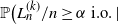 $\mathbb{P}\big({L^{(k)}_n}/{n} \geq \alpha \text{ i.o.} \mid \,$
survival
 $\big) = 0$
. Therefore, for any
 $\alpha \in (\alpha^\ast, 1)$
,
 $\limsup_{n\to\infty}({L^{(k)}_n}/{n}) \leq \alpha$
a.s. on survival and hence
 \begin{equation} \limsup_{n \to \infty}\frac{L^{(k)}_n}{n} \leq \alpha^\ast \end{equation}
a.s. on survival. The same argument applies to
 $\hat{L}^{(k)}_n$
and
 $\tilde{L}^{(k)}_n$
.
On the other hand, we may take any
 $\alpha \in (0, \alpha^\ast)$
and let
 $\delta = 1-{\alpha}/{\alpha^\ast}$
(so that
 $\alpha = \alpha^\ast (1- \delta)$
). Then
 $\big\{N_n^{\alpha n} < k\big\} \subseteq \bigcap_{j=1}^{N_{\delta n}}\big\{N_{(1-\delta)n}^{\alpha n}(j) < k\big\}$
, where
 $N_{(1-\delta)n}^{\alpha n}(j) = N_{(1-\delta)n}^{\alpha^\ast(1-\delta)n}(j)$
are the numbers of pendant edges of length
 $\geq \alpha n$
in subtrees
 $\mathcal{T}_{(1-\delta)n}(j)$
initiated by particles
 $j = 1,2,\ldots,N_{\delta n}$
at time
 $\delta n$
and evolved up to time n. Then we check that
 \begin{align*} \mathbb{P}\bigg(\frac{L_n^{(k)}}{n} < \alpha, N_{\delta n} > n\bigg) = \mathbb{P}\big(N_n^{\alpha n} < k, N_{\delta n} > n\big) & \leq \mathbb{P}\Bigg(\bigcap_{j=1}^{N_{\delta n}}\big\{N_{(1-\delta)n}^{\alpha n}(j) < k\big\}, N_{\delta n} > n\Bigg) \\ & = \mathbb{E}\big[\big(\mathbb{P}\big(N_{(1-\delta)n}^{\alpha n} < k\big)\big)^{N_{\delta n}} \mathbf{1}_{\{N_{\delta n} > n\}}\big] \\ & \leq \mathbb{P}\big(N_{(1-\delta)n}^{\alpha^\ast(1-\delta)n} < k\big)^n\mathbb{P}\big(N_{\delta n} > n\big). \end{align*}
Since
 $\mathbb{P}\big(N_{(1-\delta)n}^{\alpha^\ast(1-\delta)n} < k\big) \to \mathbb{P}(V_0 < k) < 1$
as
 $n \to \infty$
, it follows that
 $\mathbb{P}\big({L_n^{(k)}}/{n} < \alpha, N_{\delta n} > n\big)$
is summable over n. Therefore
 $\mathbb{P}\big({L_n^{(k)}}/{n} < \alpha, N_{\delta n} > n \text{ i.o.}\big) = 0$
and so also
 \[ \mathbb{P}\bigg(\frac{L_n^{(k)}}{n} < \alpha, N_{\delta n} > n \text{ i.o.} \mid \text{survival}\bigg) = 0. \]
Since
 $\mathbb{P}\big(N_{\delta n} > n \text{ eventually} \mid \text{survival}\big) = 1$
, it must be that
 $\mathbb{P}\big({L_n^{(k)}}/{n} < \alpha \text{ i.o.} \mid \text{survival}\big) = 0$
, and thus
 $\liminf_{n\to\infty}({L_n^{(k)}}/{n}) \geq \alpha$
a.s. on survival for all
 $\alpha\in(\alpha^\ast,1)$
. Therefore,
 \begin{equation} \liminf_{n \to \infty} \frac{L_n^{(k)}}{n} \geq \alpha^\ast \end{equation}
a.s. on survival, and the same argument applies to
 $\hat{L}_n^{(k)}$
and
 $\tilde{L}_n^{(k)}$
. Putting together (30) and (31), we see that
 \[ \lim_{n\to\infty}\frac{L_n^{(k)}}{n} = \lim_{n\to\infty}\frac{\hat{L}_n^{(k)}}{n} = \lim_{n\to\infty}\frac{\tilde{L}_n^{(k)}}{n} = \alpha^\ast \]
a.s. on survival.
Proof of convergence in Theorem
2 along the reals. The key observations are that for any times
 $s \leq t$
it is true that
 $L_t^{(k)} \leq L_s^{(k)} + (t-s)$
(since over the time interval [s,t] the kth-longest pendant edge cannot increase by more than
 $t-s$
),
 $\hat{L}_s^{(k)} \leq \hat{L}_t^{(k)}$
, and
 $\tilde{L}_s^{(k)} \leq \tilde{L}_t^{(k)}$
(since the kth-longest edge and kth-longest interior edge cannot get shorter over time). Thus, for any
 $t \in [0, \infty)$
it is true that
 \begin{align*} & \frac{L_{\lceil t \rceil}^{(k)}}{\lceil t \rceil} \cdot \frac{\lceil t \rceil}{t} - \frac{1}{t} = \frac{L_{\lceil t \rceil}^{(k)} - 1}{t} \leq \frac{L_t^{(k)}}{t} \leq \frac{L_{\lfloor t \rfloor}^{(k)} + 1}{t} = \frac{L_{\lfloor t \rfloor}^{(k)}}{\lfloor t \rfloor} \cdot \frac{\lfloor t \rfloor}{t} + \frac{1}{t}, \\ & \frac{\hat{L}_{\lfloor t \rfloor}^{(k)}}{\lfloor t \rfloor} \cdot \frac{\lfloor t \rfloor}{t} = \frac{\hat{L}_{\lfloor t \rfloor}^{(k)}}{t} \leq \frac{\hat{L}_t^{(k)}}{t} \leq \frac{\hat{L}_{\lceil t \rceil}^{(k)}}{t} = \frac{\hat{L}_{\lceil t \rceil}^{(k)}}{\lceil t \rceil} \cdot \frac{\lceil t \rceil}{t}, \\ & \frac{\tilde{L}_{\lfloor t \rfloor}^{(k)}}{\lfloor t \rfloor} \cdot \frac{\lfloor t \rfloor}{t} = \frac{\tilde{L}_{\lfloor t \rfloor}^{(k)}}{t} \leq \frac{\tilde{L}_t^{(k)}}{t} \leq \frac{\tilde{L}_{\lceil t \rceil}^{(k)}}{t} = \frac{\tilde{L}_{\lceil t \rceil}^{(k)}}{\lceil t \rceil} \cdot \frac{\lceil t \rceil}{t}. \end{align*}
Taking
 $t \to \infty$
yields the results.
Funding Information
Sergey Bocharov was partially funded by the Research Development Fund of Xi’an Jiaotong-Liverpool University (RDF-23-01-134). Simon Harris would like to acknowledge the support from the New Zealand Royal Society Te Apārangi Marsden Fund (22-UOA-052) during this research.
Competing Interests
There were no competing interests to declare which arose during the preparation or publication process of this article.