Condition numbers were independently introduced by Alan Turing (Reference Turing1948) and by John von Neumann and Herman Goldstine (Reference von Neumann and Goldstine1947) as a tool in their efforts to understand the accuracy (or equivalently the loss of precision) in the solution of linear systems in the presence of finite-precision arithmetic. Very shortly thereafter, Magnus Hestenes and Eduard Stiefel (Reference Hestenes and Stiefel1952) showed that these condition numbers played a central role in the determination of the speed of convergence of the conjugate gradient method, thus adding time to accuracy in the list of features that appeared to be controlled, at least partially, by the condition of the input data.
During the more than sixty years that followed the publication of these fundamental articles, condition numbers became pervasive characters in the literature of numerical algorithms. Unfortunately, this ubiquity of condition numbers is balanced by some difficulty in nailing them down: it appears that computing the condition number of an input, for a given problem, is no easier than solving the problem for this particular input. A programme that emerged from this situation – going back to Goldstine and von Neumann (Reference Goldstine and von Neumann1951) and strongly advocated by James Demmel (Reference Demmel1988) and Steve Smale (Reference Smale and Iserles1997) among others – was to focus on the behaviour of an algorithm for a typical input, rather than for a specific one. Such analysis would allow one to ascertain how well the algorithm behaves in general. To implement this approach, one would select an algorithmic feature to be analysed (say time or loss of precision), obtain bounds for this feature in terms of a relevant condition number, and then, having endowed the space of inputs with a probability measure, derive results for the behaviour above in the form of either expectations or probability tails for the selected algorithmic feature. A recent twist in this programme, known as smoothed analysis and championed by Daniel Spielman and Shang-Hua Teng (Reference Spielman and Teng2002), shifted the focus from a typical input to a typical small perturbation of an arbitrary input.
The following pages offer an overview of the development of this programme. Like Julius Caesar’s Gaul (book I, ch. 1), this paper is divided into three parts. In Section 1 we give a summary of condition numbers that focuses on how are they defined in various frameworks. In Section 2 we do the same for the two forms of probabilistic analysis we mentioned above. Finally, in Section 3, we provide examples of problems and algorithms for which this condition-based analysis has been implemented.
The subject of this overview has been given a detailed treatment in the recent book by Bürgisser and Cucker (Reference Bürgisser and Cucker2013), and most of the concepts, methods and results herein can be further explored there. A notable exception is the material in Sections 3.8(g) and 3.9.
1 A brief introduction to condition numbers
1.1 Condition and accuracy
Assume we want to compute a function  ${\it\varphi}$ via a computer algorithm
 ${\mathcal{A}}^{{\it\varphi}}$. In the simplest possible setting,
 $$\begin{eqnarray}{\it\varphi}:\mathbb{R}^{m}\rightarrow \mathbb{R}^{q}.\end{eqnarray}$$
If computations are going to be done with finite precision only, the point  $\widetilde{{\it\varphi}(a)}$ returned by
 ${\mathcal{A}}^{{\it\varphi}}$ will be just an approximation of
 ${\it\varphi}(a)$, for every
 $a\in \mathbb{R}^{m}$. The immediate relevant question is, how good is this approximation?
Leaving aside, for the moment, the fact that to answer this question we need a way of measuring the quality of an approximation, our starting point is the fact that, historically, this problem has been split into two simpler problems. On the one hand, we seek to determine how well the algorithm  ${\mathcal{A}}^{{\it\varphi}}$ computes
 ${\it\varphi}$. That is, how badly does
 ${\mathcal{A}}^{{\it\varphi}}$ accumulate errors? On the other hand, we attempt to estimate the sensitivity of the data
 $a$ with respect to
 ${\it\varphi}$. That is, how much does
 ${\it\varphi}(a)$ change when
 $a$ is slightly perturbed? Condition numbers are numerical answers to this last question.
A fairly general definition of the (absolute) condition number  $\mathsf{acond}^{{\it\varphi}}(a)$ of
 $a$ with respect to
 ${\it\varphi}$ would be
 $$\begin{eqnarray}\mathsf{acond}^{{\it\varphi}}(a):=\lim _{{\it\delta}\rightarrow 0}\sup _{\mathsf{Error}(\tilde{a})\leq {\it\delta}}\frac{\mathsf{Error}({\it\varphi}(\tilde{a}))}{\mathsf{Error}(\tilde{a})},\end{eqnarray}$$
where the numerator and denominator in the fraction measure the size of the error in the output  ${\it\varphi}(\tilde{a})$ and the input perturbation
 $\tilde{a}$, respectively. These measures can be componentwise or normwise, and in the latter case, still vary depending on the selected norm. In addition, relative errors can be considered instead of absolute errors, in which case the (relative) condition number
 $\mathsf{cond}^{{\it\varphi}}(a)$ of
 $a$ with respect to
 ${\it\varphi}$ takes the form
 $$\begin{eqnarray}\mathsf{cond}^{{\it\varphi}}(a):=\lim _{{\it\delta}\rightarrow 0}\sup _{\mathsf{RelError}(\tilde{a})\leq {\it\delta}}\frac{\mathsf{RelError}({\it\varphi}(\tilde{a}))}{\mathsf{RelError}(\tilde{a})}.\end{eqnarray}$$
The ultimate choice for all these possibilities will have to depend on the situation at hand (and the examples in Section 3 below will make this clear). A common feature for all those choices, however, is the presence of ill-posed data. These are the elements  $a\in \mathbb{R}^{m}$ for which the limit in (1.2) or (1.3) is infinite, the set of which is usually denoted by
 ${\rm\Sigma}$.
Some of these choices lead to well-known objects. Thus, in the case when  ${\it\varphi}$ is differentiable and we measure the size of both the input perturbation and the error in the output using (Euclidean) norms, the absolute condition number
 $\mathsf{acond}^{{\it\varphi}}(a)$ becomes
 $$\begin{eqnarray}\mathsf{acond}^{{\it\varphi}}(a)=\lim _{{\it\delta}\rightarrow 0}\sup _{\Vert a-\tilde{a}\Vert \leq {\it\delta}}\frac{\Vert {\it\varphi}(a)-{\it\varphi}(\tilde{a})\Vert }{\Vert a-\tilde{a}\Vert }=\Vert D{\it\varphi}(a)\Vert ,\end{eqnarray}$$
and the corresponding relative condition number is therefore given by
 $$\begin{eqnarray}\mathsf{cond}^{{\it\varphi}}(a)=\Vert D{\it\varphi}(a)\Vert \frac{\Vert a\Vert }{\Vert {\it\varphi}(a)\Vert }.\end{eqnarray}$$
Condition numbers, however, come in more guises than the equalities above suggest. The simple reason is that not all computational problems consist in computing a differentiable function. We next briefly describe some alternative situations.
(a) Multiple-valued functions.
We use this to refer to situations where given input data may have many possible (and equally valid) outputs. For instance, given a complex univariate polynomial  $P$, compute a zero
 ${\it\zeta}$ of
 $P$. If
 $P$ has degree
 $d$ then it has at most
 $d$ zeros (and, generically, it has exactly
 $d$ zeros) and any of them is a possible output of a zero-finding algorithm. If
 ${\it\zeta}_{1},\ldots ,{\it\zeta}_{d}$ are these zeros, then definition (1.2) (or (1.3)) yields a measure of condition
 $\mathsf{acond}(P,{\it\zeta}_{i})$ for each one of them. But how does one define the condition of
 $P$? There is no canonical way to do so. But three possibilities arise by taking the best, worst, or average condition for
 $P$ over its zeros.
More generally, for an input  $a$, let
 $\mathsf{Sol}(a)$ be its associated set of solutions (i.e. all the possible outputs for
 $a$). If for each
 $y\in \mathsf{Sol}(a)$ we have a number
 ${\it\xi}(a,y)$ quantifying the condition of
 $a$ with respect to
 $y$, we may define the condition
 ${\it\xi}(a)$ of
 $a$ by taking any of the following options:
 $$\begin{eqnarray}{\it\xi}(a):=\inf _{y\in \mathsf{Sol}(a)}{\it\xi}(a,y),\quad {\it\xi}(a):=\underset{y\in \mathsf{Sol}(a)}{\mathbb{E}}{\it\xi}(a,y),\quad {\it\xi}(a):=\sup _{y\in \mathsf{Sol}(a)}{\it\xi}(a,y),\end{eqnarray}$$
where the expectation in the middle expression is for some distribution on  $\mathsf{Sol}(A)$. Which of the three we choose will depend on the problem at hand, and sometimes on the algorithmic approach we use to solve it.
(b) Condition on manifolds.
Another way in which the setting (1.1) may be too restrictive has to do with the spaces where data and outputs live. As well as the obvious fact that  ${\it\varphi}$ may be only partially defined, for a number of problems these spaces are manifolds more general than Euclidean spaces. For instance, if
 $({\it\lambda},v)$ is an eigenpair of a matrix
 $A\in \mathbb{C}^{n\times n}$, the eigenvector
 $v$ naturally lives in the projective space
 $\mathbb{P}(\mathbb{C}^{n})$, which motivates the following general framework for condition numbers.
Let  $X$ be a manifold of inputs,
 $Y$ a manifold of outputs, and let
 $V\subseteq X\times Y$ be a submanifold of ‘solutions’ to some computational problem. We assume that
 $X$ and
 $V$ have the same dimension
 $n$ to guarantee a local uniqueness of solutions. Consider the projection
 ${\it\pi}_{1}:V\rightarrow X,(x,y)\mapsto x$, and its derivative
 $D{\it\pi}_{1}(x,y):T_{(x,y)}V\rightarrow T_{x}X$, which is the restriction of the projection
 $$\begin{eqnarray}T_{x}X\times T_{y}Y\rightarrow T_{x}X,\quad ({\dot{x}},{\dot{y}})\mapsto {\dot{x}},\end{eqnarray}$$
to the subspace  $T_{(x,y)}V$. We define the set of ill-posed solutions as
 $$\begin{eqnarray}{\rm\Sigma}^{\prime }:=\big\{(x,y)\in V\mid \mathsf{rank}\,D{\it\pi}_{1}(x,y)<\dim X\big\}.\end{eqnarray}$$
If  $(x_{0},y_{0})\in V\setminus {\rm\Sigma}^{\prime }$, then
 $D{\it\pi}_{1}(x_{0},y_{0}):T_{(x_{0},y_{0})}V\rightarrow T_{x_{0}}X$ is a linear isomorphism. The implicit function theorem shows that
 ${\it\pi}_{1}:V\rightarrow X$ can be locally inverted around
 $(x_{0},y_{0})$. Its inverse
 $x\mapsto (x,G(x))$ is given by the solution map
 $G:X\supseteq U\rightarrow Y$ defined on an open neighbourhood
 $U$ of
 $x_{0}$. So we have
 $(x,G(x))\in V$ for all
 $x\in U$. The derivative
 $$\begin{eqnarray}DG(x_{0}):T_{x_{0}}X\rightarrow T_{y_{0}}Y\end{eqnarray}$$
will be called the condition map. The inverse of  $D{\it\pi}_{1}(x_{0},y_{0})$ is given by
 $$\begin{eqnarray}T_{x_{0}}X\rightarrow T_{(x_{0},y_{0})}V,\quad {\dot{x}}\mapsto ({\dot{x}},DG(x_{0})({\dot{x}})).\end{eqnarray}$$
A common situation is that in which  $V$ is given as the zero set of a smooth map
 $F:X\times Y\rightarrow \mathbb{R}^{n}$. In this case we have the following characterization of
 ${\rm\Sigma}^{\prime }$, in terms of the function
 $F$ itself,
 $$\begin{eqnarray}{\rm\Sigma}^{\prime }=\big\{(x,y)\in V\mid \mathsf{rank}\,\partial F/\partial y(x,y)<n\big\}.\end{eqnarray}$$
Here the partial derivative  $\partial F/\partial y(x,y):T_{y}Y\rightarrow \mathbb{R}^{n}$ is defined as the restriction of
 $DF(x,y)$ to
 $T_{y}Y$.
Now suppose that  $X$ and
 $Y$ are Riemannian manifolds. That is, we have an inner product on each tangent space
 $T_{x}X$ and
 $T_{y}Y$ that varies smoothly with
 $x$ and
 $y$, respectively. In particular,
 $T_{x}X$ and
 $T_{y}Y$ are normed vector spaces. In this case, we may define the (absolute) normwise condition number
 $$\begin{eqnarray}\mathsf{acond}^{G}(x_{0}):=\Vert DG(x_{0})\Vert =\max _{\Vert {\dot{x}}\Vert =1}\Vert DG(x_{0})({\dot{x}})\Vert\end{eqnarray}$$
as the operator norm of  $DG(x_{0})$. We note that in this general framework, it does not make sense to define relative condition numbers. However, implicitly, we can model relative notions of condition numbers by choosing the manifolds appropriately. For instance, working with projective spaces means studying ratios, which accounts for a relative notion.
This framework relates to our previous discussion. For an element  $x_{0}$ in the manifold of inputs
 $X$ we have finitely many points
 $(x_{0},y_{1}),\ldots ,(x_{0},y_{s})$ in the fibre
 ${\it\pi}_{1}^{-1}(x_{0})$. Each of them has a corresponding solution map
 $G_{j}$,
 $j=1,\ldots ,s$, and a condition number
 $\mathsf{acond}^{G_{j}}(x_{0})$. The condition of
 $x_{0}$ will depend on the computational problem we are considering associated with the geometric situation
 $V\subseteq X\times Y$. As described in (a) above, the three typical choices are
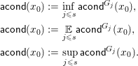 $$\begin{eqnarray}\displaystyle \mathsf{acond}(x_{0}) & := & \displaystyle \inf _{j\leq s}\mathsf{acond}^{G_{j}}(x_{0}),\nonumber\\ \displaystyle \mathsf{acond}(x_{0}) & := & \displaystyle \underset{j\leq s}{\mathbb{E}}\mathsf{acond}^{G_{j}}(x_{0}),\nonumber\\ \displaystyle \mathsf{acond}(x_{0}) & := & \displaystyle \sup _{j\leq s}\mathsf{acond}^{G_{j}}(x_{0}).\nonumber\end{eqnarray}$$
Note that the last two choices force us to define the set of ill-posed inputs to be the set  ${\rm\Sigma}:={\it\pi}_{1}({\rm\Sigma}^{\prime })$, whereas the first choice requires
 $$\begin{eqnarray}{\rm\Sigma}:=\big\{x\in X\mid (x,y)\in {\rm\Sigma}^{\prime }\text{for all }(x,y)\in {\it\pi}^{-1}(x)\big\}.\end{eqnarray}$$
(c) Finite-valued functions.
Here we consider a function  ${\it\varphi}:\mathbb{R}^{m}\rightarrow Y$ where
 $Y$ is a finite set (say
 $Y=\{y_{1},\ldots ,y_{k}\}$). In this situation the quantity
 $\mathsf{acond}^{{\it\varphi}}(a)$ in (1.2) is of little use. It is immediate to check that
 $\mathsf{acond}^{{\it\varphi}}(a)=\infty$ when
 $a$ is in the boundary of some
 $S_{j}:=\{a\in \mathbb{R}^{m}\mid {\it\varphi}(a)=y_{j}\}$, for
 $j=1,\ldots ,k$, and that
 $\mathsf{acond}^{{\it\varphi}}(a)=0$ otherwise.
The union  ${\rm\Sigma}$ of the boundaries between the sets
 $S_{j}$ is composed of data
 $a$ for which there is no hope that a finite-precision computation with input
 $a$ will yield a reliable output.
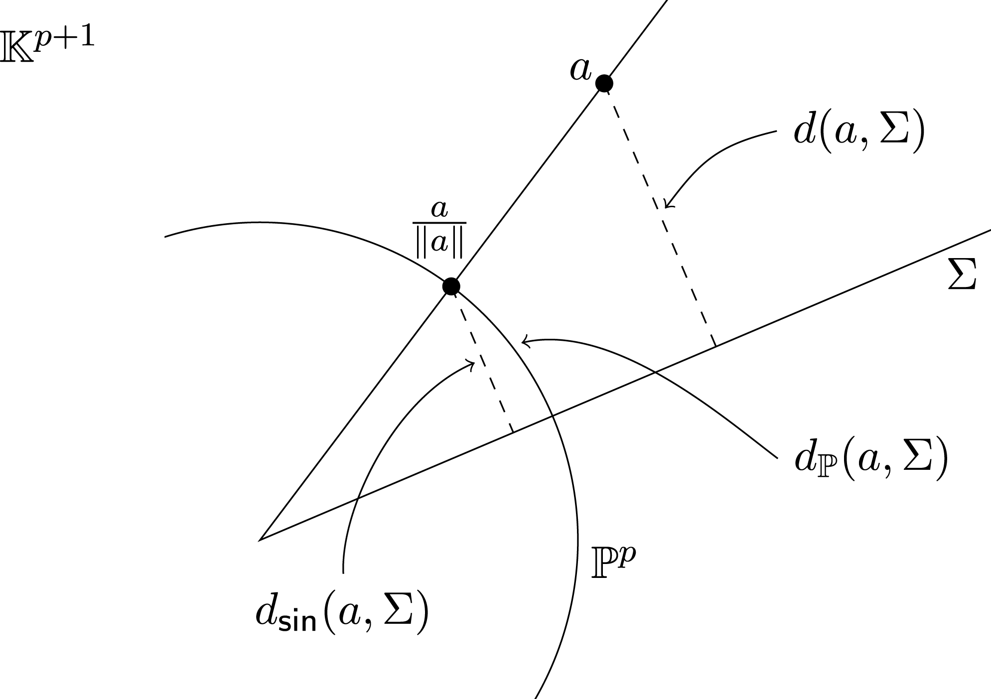
An idea championed by Jim Renegar (Reference Renegar1994b, Reference Renegar1995a, Reference Renegar1995b) is to define the condition for finite-valued problems to be the inverse of the distance to ill-posedness, that is,
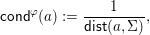 $$\begin{eqnarray}\mathsf{cond}^{{\it\varphi}}(a):=\frac{1}{\mathsf{dist}(a,{\rm\Sigma})},\end{eqnarray}$$
or a relative inverse distance
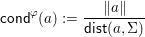 $$\begin{eqnarray}\mathsf{cond}^{{\it\varphi}}(a):=\frac{\Vert a\Vert }{\mathsf{dist}(a,{\rm\Sigma})}\end{eqnarray}$$
if the scaling properties of the problem suggest that this is better, which is often the case. Other approaches to defining conditions for these problems have been used as well.
Notable within the class of finite-valued problems is the subclass of decision problems. These consist of a question whose answer is either Yes or No (e.g. Is a symmetric matrix  $A$ positive semidefinite? Does a given linear programme have feasible points?) Although less relevant in the context of numerical algorithms (as opposed to their relevance to discrete computations, where they form the backbone of complexity theory) they nonetheless form a class deserving analysis.
1.2 Condition and complexity
The first problem for which a condition number was considered was matrix inversion (von Neumann and Goldstine Reference von Neumann and Goldstine1947, Turing Reference Turing1948). For an  $n\times n$ matrix
 $A$, the relative condition number, usually denoted by
 ${\it\kappa}(A)$, was characterized as
 ${\it\kappa}(A)=\Vert A\Vert \,\Vert A^{-1}\Vert$. Shortly thereafter, this quantity occurred as a parameter in the complexity analysis of the conjugate gradient method. This is an iterative algorithm to calculate the solution
 $x^{\ast }$ of the linear system
 $Ax=b$, where
 $A$ is a symmetric
 $n\times n$ positive definite matrix and
 $b\in \mathbb{R}^{n}$, given an initial approximation
 $x_{0}$. Let
 $x_{k}$ denote the approximation to
 $x^{\ast }$ after
 $k$ iterations of the algorithm and let
 ${\it\varepsilon}_{k}:=\Vert x_{k}-x^{\ast }\Vert _{A}$ be the error of this approximation (with respect to a certain
 $A$-norm: see (3.13)). Then (and we will return to this in more detail in Section 3.4), the number of arithmetic operations – the cost of the execution with input matrix
 $A$ – to ensure that
 ${\it\varepsilon}_{k}\leq {\it\delta}{\it\varepsilon}_{0}$ for a given
 ${\it\delta}>0$ can be shown to be
 $O(n^{2}\sqrt{{\it\kappa}(A)}\ln (1/{\it\delta}))$.
This situation – the fact that the cost of an iterative algorithm, even assuming infinite precision, depends on the condition number of the input – turned out to be pervasive.
2 A brief introduction to probabilistic analysis
A general feeling among researchers is that computing a condition number is no easier than computing the corresponding function. An attempt to make this feeling precise was given by Renegar (Reference Renegar1994a). A different approach (Cheung and Cucker Reference Cheung and Cucker2005) showed that this is the case for all condition numbers given by (1.7) – which we will call conic. The value of condition numbers thus appears to be questionable: they provide useful information on the difficulty of computing a function but they are at least as difficult to compute as the function itself.
A first way out of this quandary was proposed almost as early as condition numbers themselves. Goldstine and von Neumann (Reference Goldstine and von Neumann1951), in a sequel to their founding paper (von Neumann and Goldstine Reference von Neumann and Goldstine1947), endowed the set of  $n\times n$ real matrices with a probability measure and estimated the probability that ‘an approximate inverse’ is found; they concluded that this ‘will usually’ be the case provided
 $n$ is not too large. The particular bounds for
 $n$ (as a function of the desired precision) are of no consequence here; these bounds have been much improved since then. The overall idea, in contrast, is of paramount importance. Instead of focusing on the difficulty of particular instances of a problem (e.g. specific
 $n\times n$ matrices), Goldstine and von Neumann proposed that one should attempt to understand how difficult the problem is in general (e.g. how difficult it is to invert general
 $n\times n$ matrices). In other words, instead of computing condition numbers for a specific instance, one aims at probabilistic estimates for the condition number of random instances. These estimates usually take the form of either an expectation or a probability tail, and a sense of the difficulty of the problem is derived from their order of growth with respect to the size or dimension of the problem (the integer
 $n$ in the example above). That the latter was the goal was clear in the paper of Goldstine and von Neumann. They write that ‘the coefficients … are probably not optimal, but result from the crudeness of our probabilistic techniques. However, our principal aim was not to produce “best possible” estimates, but was merely to obtain a feeling for the sizes of the errors likely to be encountered’ (Goldstine and von Neumann Reference Goldstine and von Neumann1951, p. 201).
The approach outlined above received a strong push in the work of Jim Demmel in the late 1980s. First (see Demmel Reference Demmel1987) he showed that for many problems, the condition number defined in (1.3) can be either characterized by the expression in (1.7) or bounded by a small multiple of this expression. The import of this paper was thus that many problems admit conic condition numbers. Then (see Demmel Reference Demmel1988) he gave bounds for the expectation of conic condition numbers. These bounds were general and expressed in terms of the dimension of the ambient space and the degree and codimension of the set  ${\rm\Sigma}$. We will return to this subject, and give more details, in Section 3.10.
Demmel’s work was motivated by issues relating to finite precision. But the idea of understanding the ‘typical’ behaviour of an algorithm through a probabilistic analysis of its condition number naturally applies to complexity as well. Steve Smale (Reference Smale and Iserles1997) proposed a general approach to the complexity of numerical problems. It consisted of first providing bounds for an algorithm’s cost in terms of both the size and condition of the input, and then removing the condition from these bounds by replacing them with probabilistic estimates.
Whether for accuracy or complexity analyses, probabilistic estimates will rely on the underlying probability measure assumed. In addition, they depend on what exactly the randomization of the input is meant to capture.
The current literature exhibits two different ideas for the latter. In the first one, called average analysis, data are assumed to be drawn from ‘evenly spread’ distributions. The analysis performed for such a randomization is meant to describe the behaviour of the analysed quantity for ‘typical’ data.
The second idea for randomization, known as smoothed analysis, replaces this average data with a small random perturbation of worst-case data. That is, it considers an arbitrary element  $\overline{a}$ in
 $\mathbb{R}^{m}$ (and thus, in particular, the instance at hand) and assumes that
 $\overline{a}$ is affected by random noise. The distribution for this perturbed input is usually taken to be centred and isotropic around
 $\overline{a}$, and assumed to have a small variance.
(a) Average analysis.
Most of the condition numbers occurring in the literature are scale-invariant, that is, they satisfy  $\mathsf{cond}(a)=\mathsf{cond}({\it\lambda}a)$ for all
 $a\in \mathbb{R}^{m}$ and
 ${\it\lambda}\in \mathbb{R}\setminus \{0\}$. We will therefore confine our discussion to scale-invariant random variables.
We have already mentioned that the underlying distribution in average analysis is ‘evenly spread’ and that expected values for such distributions are meant to capture the behaviour of the random variable on the ‘average Joe’ inhabitant of the data space. In the context we are interested in, the probabilistic analysis of condition numbers, this data space is usually a Euclidean space  $\mathbb{R}^{m}$. So the question that poses itself is with which distribution should we endow
 $\mathbb{R}^{m}$ for the analysis. Assume we have a ‘natural’ system of coordinates in
 $\mathbb{R}^{m}$. A first step towards an answer consists in noting that such a distribution should be rotationally invariant. The undistinguished character of the ‘average Joe’ cannot favour any particular direction. Furthermore, scale invariance allows us to take a second step. Indeed, for such a function of
 $\mathbb{R}^{m}$ the value of the density along a half-line with origin at 0 is not relevant. It follows that we can take any rotationally invariant distribution on
 $\mathbb{R}^{m}$, and the collection of remarkable features of the standard Gaussian makes this distribution the obvious choice.
Scale invariance also suggests the choice of an underlying distribution that is evenly spread by definition, namely, the uniform distribution on the unit sphere  $\mathbb{S}^{m-1}$ (this requires us to consider data on the sphere only).
All the above, however, is subject to a ‘natural’ system of coordinates in  $\mathbb{R}^{m}$. And while some situations may suggest such a system, its choice remains a bone of contention for average-case analysis. The most common objection to average-case analysis is that its underlying probability measures may not accurately reflect the distributions occurring in practice, in particular, that they may be ‘optimistic’ in the sense that they may put more probability mass on the instances for which the values of the function
 ${\it\psi}$ under consideration are small. Such optimism would produce an expectation
 $\mathbb{E}{\it\psi}$ smaller than the true one.
(b) Smoothed analysis.
Smoothed analysis was introduced mainly to overcome this objection. Its underlying idea, we recall, was to look at the behaviour of a function for small perturbations of arbitrary data. In the case of a condition number, this amounts to understanding the condition of slight perturbations of ill-posed data. When compared with the average analysis, it replaces the goal of showing that
 $$\begin{eqnarray}\text{for a random}~a,\text{it is unlikely that}~\mathsf{cond}(a)~\text{will be large}\end{eqnarray}$$
by the following one:
 $$\begin{eqnarray}\displaystyle & & \displaystyle \text{for all}~\overline{a},\text{it is unlikely that a slight random perturbation}\nonumber\\ \displaystyle & & \displaystyle \overline{a}+{\rm\Delta}a~\text{of}~\overline{a}~\text{will have}~\mathsf{cond}(\overline{a}+{\rm\Delta}a)~\text{large}.\nonumber\end{eqnarray}$$
To perform a smoothed analysis, a family of distributions (parametrized by a parameter  $r$ controlling the size of the perturbation) is considered with the following characteristics:
(a) the density at a point
 $a$ depends only on the distance $\Vert a-\overline{a}\Vert$,
(b) the value of
$r$ is closely related to the variance of $\Vert a-\overline{a}\Vert$.


A first possible choice for this family of distributions is the set of Gaussians  $N(\overline{a},{\it\sigma}^{2}\,\text{Id}_{m})$. The role of
 $r$ is in this case played by
 ${\it\sigma}>0$. Because of scale invariance, one usually assumes that the base point
 $\overline{a}$ lives in
 $\mathbb{S}^{m-1}$. In this way, the value of the parameter
 ${\it\sigma}$ controlling the size of the perturbations is directly comparable with the size of
 $\overline{a}$.
A different choice of distributions consists in taking  $\overline{a}\in \mathbb{S}^{m-1}$ and, for each
 $r\in (0,{\it\pi}]$, the uniform measure on the spherical cap,
 $$\begin{eqnarray}\mathsf{cap}(\overline{a},r):=\{x\in \mathbb{S}^{m-1}\mid \langle x,\overline{a}\rangle \geq \cos r\}.\end{eqnarray}$$
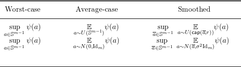
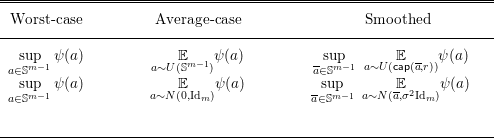
Table 2.1 shows a schematic comparison of the quantities computed in worst-case, average-case, and smoothed analyses for a scale-invariant function  ${\it\psi}:\mathbb{R}^{m}\rightarrow \mathbb{R}$ in both the uniform and Gaussian cases. Usually, the quantities estimated in the first two columns are functions of
 $m$. For the estimate in a smoothed analysis there is, in addition, a dependence on
 $r$ or
 ${\it\sigma}$. This dependence appears to interpolate between worst-case and average-case. Indeed, in the uniform case, when
 $r$ approaches 0, the value of
 $$\begin{eqnarray}\sup _{\overline{a}\in \mathbb{S}^{m-1}}\underset{a\sim U(\mathsf{cap}(\overline{a},r))}{\mathbb{E}}{\it\psi}(a)\end{eqnarray}$$
approaches  $\sup _{a\in \mathbb{R}^{m}}{\it\psi}(a)$, while when
 $r={\it\pi}$ it equals
 $\mathbb{E}_{a\sim U(\mathbb{S}^{m-1})}{\it\psi}(a)$ (since
 $\mathsf{cap}(\overline{a},{\it\pi})=\mathbb{S}^{m-1}$ for all
 $\overline{a}$). A similar situation holds in the Gaussian framework.
The local nature of randomization in smoothed analysis, coupled with its worst-case dependence on the input data, removes from smoothed analysis the objection to average-case analysis mentioned above. A satisfying result in this context (usually a low-degree polynomial bound in the input size  $m$ and in the inverse of the dispersion parameter
 $r$) is consequently considered a more reliable indication that one may expect low values for the function
 ${\it\psi}$ in practice. In addition, there is an emerging impression that smoothed analysis is robust in the sense that its dependence on the chosen family of measures is low.
Notation.
In all that follows, we will omit the subindex  $m$ denoting dimension in
 $\text{Id}_{m}$. These dimensions are always clear from the context.
3 A repertoire of examples
In this last section – the longest in this overview – we summarize for a number of examples the role played by a condition number in the evaluation of some measure of algorithmic performance, and the way a probabilistic analysis (average or smoothed) allows for a direct assessment of this evaluation. The goal is not to prove all, or even most, of the results described (due to obvious space limitations), let alone to prove the sharpest possible results (for most of them such a proof would be too long, and interesting to only a few specialists). Instead we want to offer a catalogue as broad as possible of instances of the general framework sketched in the preceding sections. To do so, we have chosen to give full proofs for a few results we believe foundational, to sketch the proofs of some recent breakthroughs, and to simply state, omitting proofs, some state-of-the-art technical results. The division between these three categories is, needless to say, a personal choice.
In all cases we indicate references in the literature where notions have been developed, algorithms designed, and theorems established. As well as these references, a recurring source is the recent book by Bürgisser and Cucker (Reference Bürgisser and Cucker2013), where most of the themes we deal with in this overview are given full-length discussion.
The problems of inverting matrices or solving linear systems engendered condition numbers; a lively narrated story of the events that led Turing to his pioneer paper (Turing Reference Turing1948) is given by Wilkinson (Reference Wilkinson1971). The same reasons (I will not spell them out here) also explain why the condition number for these problems is ubiquitous in the literature – and why we will devote some time to it.
3.1 Linear systems
(a) Loss of precision.
Assume we are solving the system  $Ax=b$ (or inverting the matrix
 $A$) with a real-number algorithm
 ${\mathcal{A}}$ executed using floating-point arithmetic, and let
 ${\it\epsilon}_{\mathsf{mach}}$ be the epsilon-machine (or round-off unit) at hand (for a primer on finite-precision computations see Higham Reference Higham1996, Chapters 2 and 3). This means that all floating-point numbers occurring during the execution of
 ${\mathcal{A}}$ are rounded to
 $|\!\log {\it\epsilon}_{\mathsf{mach}}|$ significant digits (here
 $\log$ refers to logarithm in base 10). In particular, this is the precision of the entries in the data
 $(A,b)$. On the other hand, the number of correct digits in the
 $i$th component of the computed solution
 $\tilde{x}$ is approximately
 $-\log \mathsf{RelError}(\tilde{x}_{i})$, where
 $$\begin{eqnarray}\mathsf{RelError}(\tilde{x}_{i}):=\frac{\mathsf{Error}(\tilde{x}_{i})}{|x_{i}|}=\frac{|x_{i}-\tilde{x}_{i}|}{|x_{i}|}.\end{eqnarray}$$
Therefore, the value
 $$\begin{eqnarray}\mathsf{LoP}(x_{i}):=\log \frac{\mathsf{RelError}(\tilde{x}_{i})}{{\it\epsilon}_{\mathsf{mach}}}=|\!\log {\it\epsilon}_{\mathsf{mach}}|-|\!\log \mathsf{RelError}(\tilde{x}_{i})|\end{eqnarray}$$
quantifies the loss of precision in the computation of  $x_{i}$. If we take the precision of
 $\tilde{x}$ to be
 $$\begin{eqnarray}-\log \mathsf{RelError}(\tilde{x}):=-\log \frac{\Vert x-\tilde{x}\Vert }{\Vert x\Vert },\end{eqnarray}$$
then the loss of precision in the computation of  $x$ is
 $$\begin{eqnarray}\mathsf{LoP}(x):=\log \frac{\mathsf{RelError}(\tilde{x})}{{\it\epsilon}_{\mathsf{mach}}}=|\!\log {\it\epsilon}_{\mathsf{mach}}|+\log \mathsf{RelError}(\tilde{x}).\end{eqnarray}$$
Next assume that algorithm  ${\mathcal{A}}$ corresponds to computing
 $x$ via the Householder QR factorization method. The following result is a well-known backward error analysis for this algorithm (see Higham Reference Higham1996, Theorem 19.3).
In all that follows, for any square matrix  $M$,
 $\Vert M\Vert _{F}$ and
 $\Vert M\Vert$ denote the Frobenius and spectral norms of
 $M$, respectively.
Theorem 3.1. Let  $A\in \mathbb{R}^{n\times n}$ be invertible and
 $b\in \mathbb{R}^{n}$. If the system
 $Ax=b$ is solved using the Householder QR factorization method, then the computed solution
 $\tilde{x}$ satisfies
 $$\begin{eqnarray}\tilde{A}\tilde{x}=\tilde{b},\end{eqnarray}$$
where  $\tilde{A}$ and
 $\tilde{b}$ satisfy the relative error bounds
 $$\begin{eqnarray}\Vert \tilde{A}-A\Vert _{F}\leq n{\it\gamma}_{sn}\Vert A\Vert _{F}\quad \text{and}\quad \Vert \tilde{b}-b\Vert \leq n{\it\gamma}_{sn}\Vert b\Vert\end{eqnarray}$$
for a small constant  $s$ and with
 ${\it\gamma}_{k}:=k{\it\epsilon}_{\mathsf{mach}}/(1-k{\it\epsilon}_{\mathsf{mach}}).$ ◻
We can tie this result to the general discussion on condition numbers in Section 1.1. To do so, we define the set of ill-posed matrices
 $$\begin{eqnarray}{\rm\Sigma}:=\{A\in \mathbb{R}^{n\times n}\mid \det (A)=0\},\end{eqnarray}$$
write  ${\mathcal{D}}:=\mathbb{R}^{n\times n}\setminus {\rm\Sigma}$ and let
 ${\it\varphi}:{\mathcal{D}}\times \mathbb{R}^{n}\rightarrow \mathbb{R}^{n}$ be given by
 ${\it\varphi}(A,b)=A^{-1}b$. Taking
 $$\begin{eqnarray}\mathsf{RelError}(\tilde{A},\tilde{b}):=\max \biggl\{\frac{\Vert \tilde{A}-A\Vert }{\Vert A\Vert },\frac{\Vert \tilde{b}-b\Vert }{\Vert b\Vert }\biggr\},\end{eqnarray}$$
Theorem 3.1 (and the bound  $\Vert \cdot \Vert _{F}\leq \sqrt{n}\Vert \cdot \Vert$) shows that
 $\tilde{x}={\it\varphi}(\tilde{A},\tilde{b})$ with
 $$\begin{eqnarray}\mathsf{RelError}(\tilde{A},\tilde{b})\leq n^{3/2}{\it\gamma}_{sn}.\end{eqnarray}$$
We now fix a normwise measure for the relative error of  $\tilde{x}$ (i.e.
 $\mathsf{RelError}(\tilde{x}):=\Vert \tilde{x}-x\Vert /\Vert x\Vert$), consider the relative condition number
 $\mathsf{cond}^{{\it\varphi}}(A,b)$ with respect to the relative errors in both the input
 $(A,b)$ and the solution
 $x$, and set
 ${\it\epsilon}_{\mathsf{mach}}\rightarrow 0$. Then,
 ${\it\gamma}_{k}=k{\it\epsilon}_{\mathsf{mach}}+o({\it\epsilon}_{\mathsf{mach}})$ and (recall definition (1.3))
 $$\begin{eqnarray}\mathsf{RelError}(\tilde{x})\leq \mathsf{RelError}(\tilde{A},\tilde{b})\,\mathsf{cond}^{{\it\varphi}}(A,b)+o({\it\epsilon}_{\mathsf{mach}}).\end{eqnarray}$$
We conclude that this relative error satisfies
 $$\begin{eqnarray}\frac{\Vert \tilde{x}-x\Vert }{\Vert x\Vert }\leq sn^{5/2}{\it\epsilon}_{\mathsf{mach}}\mathsf{cond}^{{\it\varphi}}(A,b)+o({\it\epsilon}_{\mathsf{mach}}),\end{eqnarray}$$
and consequently, that the loss of precision is bounded by
 $$\begin{eqnarray}\mathsf{LoP}(A^{-1}b)\leq \frac{5}{2}\log n+\log \mathsf{cond}(A,b)+\log s+o(1).\end{eqnarray}$$
(b) Characterizations of$\mathsf{cond}^{{\it\varphi}}(A,b)$.

We begin by proving an assertion we claimed early in Section 1.2. Define the map  ${\it\kappa}:{\mathcal{D}}\rightarrow \mathbb{R}$ by
 $$\begin{eqnarray}{\it\kappa}(A):=\Vert A\Vert \Vert A^{-1}\Vert .\end{eqnarray}$$
Then  ${\it\kappa}(A)\geq 1$, since
 $1=\Vert \text{Id}\Vert \leq \Vert A\Vert \Vert A^{-1}\Vert ={\it\kappa}(A)$.
Theorem 3.2. Let  $\mathsf{cond}^{{\it\varphi}}(A,b)$ be as above. Then,
 $$\begin{eqnarray}\mathsf{cond}^{{\it\varphi}}(A,b)={\it\kappa}(A)+\frac{\Vert A^{-1}\Vert \Vert b\Vert }{\Vert A^{-1}b\Vert }.\end{eqnarray}$$
In particular, we have
 $$\begin{eqnarray}{\it\kappa}(A)\leq \mathsf{cond}^{{\it\varphi}}(A,b)\leq 2{\it\kappa}(A).\end{eqnarray}$$
Proof. Let  $\tilde{A}=A-E$ and
 $\tilde{b}=b+f$. By definition,
 $\Vert E\Vert \leq \mathsf{R}\Vert A\Vert$ and
 $\Vert f\Vert \leq \mathsf{R}\Vert b\Vert$, where for simplicity,
 $\mathsf{R}=\mathsf{RelError}(A,b)$. We have, for
 $\mathsf{R}\rightarrow 0$,
 $$\begin{eqnarray}\displaystyle (A-E)^{-1} & = & \displaystyle A^{-1}(\text{Id}-EA^{-1})^{-1}=A^{-1}(\text{Id}+EA^{-1}+o(\mathsf{R}))\nonumber\\ \displaystyle & = & \displaystyle A^{-1}+A^{-1}EA^{-1}+o(\mathsf{R}).\nonumber\end{eqnarray}$$
This implies, writing  $x:=A^{-1}b$ and
 $\tilde{x}:=\tilde{A}^{-1}\tilde{b}$,
 $$\begin{eqnarray}\tilde{x}-x=(A-E)^{-1}(b+f)-x=A^{-1}Ex+A^{-1}f+o(\mathsf{R}).\end{eqnarray}$$
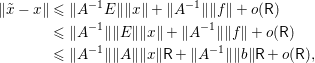
Taking norms we conclude that
 $$\begin{eqnarray}\displaystyle \Vert \tilde{x}-x\Vert & \leq & \displaystyle \Vert A^{-1}E\Vert \Vert x\Vert +\Vert A^{-1}\Vert \Vert f\Vert +o(\mathsf{R})\nonumber\\ \displaystyle & \leq & \displaystyle \Vert A^{-1}\Vert \Vert E\Vert \Vert x\Vert +\Vert A^{-1}\Vert \Vert f\Vert +o(\mathsf{R})\nonumber\\ \displaystyle & \leq & \displaystyle \Vert A^{-1}\Vert \Vert A\Vert \Vert x\Vert \mathsf{R}+\Vert A^{-1}\Vert \Vert b\Vert \mathsf{R}+o(\mathsf{R}),\nonumber\end{eqnarray}$$
and hence
 $$\begin{eqnarray}\frac{\Vert \tilde{x}-x\Vert }{\mathsf{R}\Vert x\Vert }\leq {\it\kappa}(A)+\frac{\Vert A^{-1}\Vert \Vert b\Vert }{\Vert x\Vert },\end{eqnarray}$$
which shows the upper bound in the claimed equality.
For the corresponding lower bound we choose  $y\in \mathbb{R}^{n}$ such that
 $\Vert y\Vert =1$ and
 $\Vert A^{-1}y\Vert =\Vert A^{-1}\Vert$. Further, we choose
 $v=x/\Vert x\Vert \in \mathbb{R}^{n}$ so that
 $\Vert v\Vert =1$ and
 $v^{\text{T}}x=\Vert x\Vert$. Now we put
 $$\begin{eqnarray}E:=\mathsf{R}\Vert A\Vert \,yv^{\text{T}},\quad f:=\pm \mathsf{R}\Vert b\Vert \,y.\end{eqnarray}$$
We note that
 $$\begin{eqnarray}\Vert E\Vert =\mathsf{R}\Vert A\Vert ,\quad \Vert f\Vert =\mathsf{R}\Vert b\Vert ,\end{eqnarray}$$
the first equality holding since  $\Vert yv^{\text{T}}\Vert =\Vert y\Vert \Vert v\Vert =1$. We have
 $$\begin{eqnarray}A^{-1}Ex=\mathsf{R}\Vert A\Vert \,A^{-1}y\,v^{\text{T}}x=\mathsf{R}\Vert A\Vert \Vert x\Vert A^{-1}y\end{eqnarray}$$
and hence  $\Vert A^{-1}Ex\Vert ={\it\kappa}(A)\Vert x\Vert \mathsf{R}$. Similarly,
 $A^{-1}f=\pm R\Vert b\Vert A^{-1}y$ and
 $\Vert A^{-1}f\Vert =\Vert A^{-1}\Vert \Vert b\Vert \mathsf{R}$. Since
 $A^{-1}Ex$ and
 $A^{-1}f$ are both proportional to
 $A^{-1}y$, we obtain from (3.6)
 $$\begin{eqnarray}\Vert \tilde{x}-x\Vert ={\it\kappa}(A)\Vert x\Vert \mathsf{R}+\Vert A^{-1}\Vert \Vert b\Vert \mathsf{R},\end{eqnarray}$$
if we choose the sign for  $f$ in (3.7) appropriately. This proves the claimed lower bound.
The next result shows that  ${\it\kappa}$ actually coincides with the condition number for the problem of matrix inversion.
Theorem 3.3. Let  ${\it\psi}:{\mathcal{D}}\rightarrow \mathbb{R}^{n\times n}$ be given by
 ${\it\psi}(A)=A^{-1}$. We measure the relative error on the data space and solution space with respect to spectral and Euclidean norms, respectively. Then we have
 $$\begin{eqnarray}\mathsf{cond}^{{\it\psi}}(A)={\it\kappa}(A).\end{eqnarray}$$
Proof. Let  $E\in \mathbb{R}^{n\times n}$ be such that
 $\tilde{A}=A-E$. Then
 $\mathsf{RelError}(A)=\Vert E\Vert /\Vert A\Vert$. As in the proof of Theorem 3.2, we have for
 $\Vert E\Vert \rightarrow 0$,
 $$\begin{eqnarray}\Vert \tilde{A}^{-1}-A^{-1}\Vert =\Vert A^{-1}EA^{-1}\Vert +o(\Vert E\Vert ).\end{eqnarray}$$
Hence,  $\Vert A^{-1}EA^{-1}\Vert \leq \Vert A^{-1}\Vert \Vert E\Vert A^{-1}\Vert .$ Consequently, we obtain
 $$\begin{eqnarray}\mathsf{RelError}(A^{-1})=\frac{\Vert \tilde{A}^{-1}-A^{-1}\Vert }{\Vert A^{-1}\Vert }\leq \Vert A^{-1}\Vert \Vert E\Vert +o(\Vert E\Vert )).\end{eqnarray}$$
We conclude that
 $$\begin{eqnarray}\frac{\mathsf{RelError}(A^{-1})}{\mathsf{RelError}(A)}\leq \Vert A\Vert \Vert A^{-1}\Vert +o(1)\end{eqnarray}$$
and hence  $\mathsf{cond}^{{\it\psi}}(A)\leq {\it\kappa}(A)$.
To prove the reverse inequality it is enough to find arbitrarily small matrices  $E$ such that
 $\Vert A^{-1}EA^{-1}\Vert =\Vert A^{-1}\Vert ^{2}\Vert E\Vert$, since then we can proceed from (3.8) as we did in Theorem 3.2 from (3.6).
To do so, let  $y\in \mathbb{R}^{n}$ be such that
 $\Vert y\Vert =1$ and
 $\Vert A^{-1}y\Vert =\Vert A^{-1}\Vert$. Define
 $x:=\Vert A^{-1}\Vert ^{-1}A^{-1}y$, so that
 $A^{-1}y=\Vert A^{-1}\Vert x$ and
 $\Vert x\Vert =\Vert y\Vert =1$. For any
 $B\in \mathbb{R}^{n\times n}$ we have
 $$\begin{eqnarray}\Vert A^{-1}BA^{-1}\Vert \geq \Vert A^{-1}BA^{-1}y\Vert =\Vert A^{-1}\Vert \cdot \Vert A^{-1}Bx\Vert .\end{eqnarray}$$
Since  $\Vert x\Vert =\Vert y\Vert =1$ there exists an orthogonal matrix
 $B\in \mathbb{R}^{n\times n}$ such that
 $Bx=y$. Therefore,
 $$\begin{eqnarray}\Vert A^{-1}BA^{-1}\Vert \geq \Vert A^{-1}\Vert \cdot \Vert A^{-1}y\Vert =\Vert A^{-1}\Vert ^{2}.\end{eqnarray}$$
Taking  $E={\it\delta}B$ with arbitrarily small
 ${\it\delta}$ finishes the proof.
(c) The condition number theorem.
We mentioned in Section 2 that Demmel (Reference Demmel1987) showed that many problems admit conic condition numbers. The first result of this kind, which preceded the expression ‘condition number’, was proved by Eckart and Young (Reference Eckart and Young1936). It states that for  $A\in \mathbb{R}^{n\times n}\setminus {\rm\Sigma}$, we have
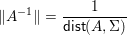 $$\begin{eqnarray}\Vert A^{-1}\Vert =\frac{1}{\mathsf{dist}(A,{\rm\Sigma})}\end{eqnarray}$$
where  $\mathsf{dist}$ is the distance induced by either the spectral or the Frobenius norm. It follows that
 $$\begin{eqnarray}{\it\kappa}(A)=\frac{\Vert A\Vert }{\mathsf{dist}(A,{\rm\Sigma})}.\end{eqnarray}$$
(d) Probabilistic analyses.
Now we prove an average analysis for  $\log {\it\kappa}(A)$. The bounds we obtain are not the sharpest possible (see Theorem 3.12) but we can use them to derive sufficiently good bounds for the average loss of precision.
For an  $n\times n$ matrix
 $A$, let
 $\hat{A}_{i}$ refer to
 $A$ with the
 $i$th column removed and, for an
 $n\times (n-1)$ matrix
 $A$ and
 $b\in \mathbb{R}^{n}$, let
 $(A,b)_{i}$ refer to the
 $n\times n$ matrix obtained from
 $A$ by inserting
 $b$ as the
 $i$th column. Also, let us denote by
 $A_{i}$ the
 $i$th column of
 $A$.
The next lemma relates the norm of the inverse of an  $n\times n$ matrix to a geometric condition on the columns of the matrix.
Lemma 3.4. Let  $A$ be an invertible
 $n\times n$ matrix. If
 $\Vert A^{-1}\Vert =x$, then there is an
 $i\in \{1,2,\ldots ,n\}$ and a vector
 $B_{i}\in \mathbb{R}^{n}$ with
 $\Vert B_{i}\Vert \leq \sqrt{n}/x$ and such that
 $A_{i}+B_{i}$ is in the space spanned by
 $A_{j},j\neq i,j\in \{1,\ldots ,n\}$.
Proof. That  $\Vert A^{-1}\Vert =x$ means that there is a unit vector
 $b\in \mathbb{R}^{n}$ such that
 $v=A^{-1}b$ and
 $\Vert v\Vert =x$. Choose
 $i$ such that
 $|v_{i}|\geq x/\sqrt{n}$. By Cramer’s rule
 $$\begin{eqnarray}v_{i}=\frac{\det (\hat{A}_{i},b)_{i}}{\det A}.\end{eqnarray}$$
Hence  $\det (\hat{A}_{i},{v_{i}}^{-1}b)_{i}=\det A$ and
 $\det (\hat{A}_{i},A_{i}-{v_{i}}^{-1}b)_{i}=0$. As the columns of
 $A$ are independent, this implies that
 $A_{i}-{v_{i}}^{-1}b$ is spanned by the other columns. Also,
 $\Vert {v_{i}}^{-1}b\Vert \leq \sqrt{n}/x$ so the statement holds for
 $B_{i}:=-{v_{i}}^{-1}b$.
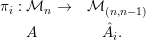
We shall let  ${\mathcal{M}}_{(n,m)}$ denote the space of real
 $n\times m$ matrices, and if
 $m=n$ we shall denote this space simply by
 ${\mathcal{M}}_{n}$. Let
 $\mathbb{S}^{n^{2}-1}\subset {\mathcal{M}}_{n}$ be the unit sphere with respect to the Frobenius norm. Also, let
 $\mathbb{B}^{n^{2}-n}$ be the unit ball in the space
 ${\mathcal{M}}_{(n,n-1)}$ and for
 $i=1,\ldots ,n$ the map
For any  ${\it\varepsilon}>0$ we consider
 $N_{{\it\varepsilon}}\subset \mathbb{S}^{n^{2}-1}$ the set of
 $A\in \mathbb{S}^{n^{2}-1}$ such that
 $A$ is not invertible or
 $\Vert A^{-1}\Vert >1/{\it\varepsilon}$. Equation (3.9) provides a geometric characterization of
 $N_{{\it\varepsilon}}$, namely
 $$\begin{eqnarray}N_{{\it\varepsilon}}=\{A\in \mathbb{S}^{n^{2}-1}\mid \mathsf{dist}_{F}(A,{\rm\Sigma})<{\it\varepsilon}\}\end{eqnarray}$$
where  $\mathsf{dist}_{F}$ is the distance in
 ${\mathcal{M}}_{n}$ induced by the Frobenius norm.
Our goal is to estimate the volume of  $N_{{\it\varepsilon}}$. To do so, consider for
 ${\it\varepsilon}>0$ and
 $i=1,\ldots ,n$ the set
 $$\begin{eqnarray}\displaystyle W_{{\it\varepsilon},i} & = & \displaystyle \big\{A\in \mathbb{S}^{n^{2}-1}\mid A_{i}\text{ is within }\sqrt{n}\,{\it\varepsilon}\text{ of the}\nonumber\\ \displaystyle & & \displaystyle \text{space spanned by the columns of }\hat{A}_{i}\big\}.\nonumber\end{eqnarray}$$
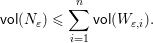
Lemma 3.5. For all  ${\it\varepsilon}>0$,
 $$\begin{eqnarray}\mathsf{vol}(N_{{\it\varepsilon}})\leq \mathop{\sum }_{i=1}^{n}\mathsf{vol}(W_{{\it\varepsilon},i}).\end{eqnarray}$$
Proof. By Lemma 3.4 we have that  $N_{{\it\varepsilon}}\subset \bigcup _{i=1}^{n}W_{{\it\varepsilon},i}$.
Now we turn to  $W_{{\it\varepsilon},i}$.
Proposition 3.6. For all  ${\it\varepsilon}>0$,
 $B\in {\mathcal{M}}_{(n,n-1)}$, and
 $i=1,\ldots ,n$, we have
 $$\begin{eqnarray}\mathsf{vol}(W_{{\it\varepsilon},i}\cap {\it\pi}_{i}^{-1}B)\leq 2\sqrt{n}\,{\it\varepsilon}\mathsf{vol}(\mathbb{S}_{(1-\Vert B\Vert _{F}^{2})^{1/2}}^{n-2}),\end{eqnarray}$$
where  $\mathbb{S}_{r}^{m-1}$ is the sphere of radius
 $r$ in
 $\mathbb{R}^{m}$.
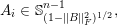
Proof. If  $A\in W_{{\it\varepsilon},i}\cap {\it\pi}_{i}^{-1}B$ then
 $\Vert A_{i}\Vert =(1-\Vert B\Vert _{F}^{2})^{1/2}$, that is,
 $$\begin{eqnarray}A_{i}\in \mathbb{S}_{(1-\Vert B\Vert _{F}^{2})^{1/2}}^{n-1},\end{eqnarray}$$
and  $A_{i}$ is within
 $\sqrt{n}{\it\varepsilon}$ of the space spanned by the columns of
 $B$.
The volume of  $W_{{\it\varepsilon},i}\cap {\it\pi}_{i}^{-1}B$ is thus at most the volume of the cylinder of base
 $\mathbb{S}_{(1-\Vert B\Vert _{F}^{2})^{1/2}}^{n-2}$ and height
 $2\sqrt{n}\,{\it\varepsilon}$.
Lemma 3.7. Let  $\mathbb{B}^{m-\ell }\subset \mathbb{R}^{m-\ell }$ be the unit ball and
 $k\geq 0$. Then
 $$\begin{eqnarray}\frac{1}{\mathsf{vol}(\mathbb{S}^{m-1})}\int _{x\in \mathbb{B}^{m-\ell }}\frac{\mathsf{vol}(\mathbb{S}_{(1-\Vert x\Vert ^{2})^{1/2}}^{k})}{(1-\Vert x\Vert ^{2})^{1/2}}\,\text{d}x_{1}\ldots \,\text{d}x_{m-\ell }=\frac{{\it\pi}^{\frac{k-\ell +1}{2}}{\it\Gamma}(\frac{m}{2})}{{\it\Gamma}(\frac{m+k-\ell +1}{2})}.\end{eqnarray}$$
Proof. The left-hand side in the statement equals
 $$\begin{eqnarray}\frac{\mathsf{vol}(\mathbb{S}^{k})}{\mathsf{vol}(\mathbb{S}^{m-1})}\int _{x\in \mathbb{B}^{m-\ell }}(1-\Vert x\Vert ^{2})^{\frac{k-1}{2}}\,\text{d}x_{1}\ldots \,\text{d}x_{m-\ell },\end{eqnarray}$$
which using spherical coordinates equals
 $$\begin{eqnarray}\frac{\mathsf{vol}(\mathbb{S}^{k})\mathsf{vol}(\mathbb{S}^{m-\ell -1})}{\mathsf{vol}(\mathbb{S}^{m-1})}\int _{0}^{1}(1-r^{2})^{\frac{k-1}{2}}\cdot r^{m-\ell -1}\,\text{d}r.\end{eqnarray}$$
Finally, using that for  $p,q\in \mathbb{R}$,
 $$\begin{eqnarray}\int _{0}^{1}t^{p}(1-t^{2})^{q}\,\text{d}t=\frac{1}{2}\frac{{\it\Gamma}(\frac{p+1}{2}){\it\Gamma}(q+1)}{{\it\Gamma}(\frac{p+1}{2}+q+1)},\end{eqnarray}$$
the fact that
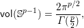 $$\begin{eqnarray}\mathsf{vol}(\mathbb{S}^{p-1})=\frac{2{\it\pi}^{p/2}}{{\it\Gamma}(\frac{p}{2})},\end{eqnarray}$$
and some elementary computations, we obtain the right-hand side.
We can now estimate the volume of  $N_{{\it\varepsilon}}$.
Proposition 3.8. For any  ${\it\varepsilon}>0$ and any
 $n\geq 2$,
 $$\begin{eqnarray}\frac{\mathsf{vol}(N_{{\it\varepsilon}})}{\mathsf{vol}(\mathbb{S}^{n^{2}-1})}\leq {\it\varepsilon}n^{5/2}.\end{eqnarray}$$
Proof. By Lemma 3.5 it suffices to show that
 $$\begin{eqnarray}\frac{\mathsf{vol}(W_{{\it\varepsilon},i})}{\mathsf{vol}(\mathbb{S}^{n^{2}-1})}\leq {\it\varepsilon}n^{3/2}.\end{eqnarray}$$
Let  ${\it\chi}_{W_{{\it\varepsilon},i}}$ be the characteristic function of
 $W_{{\it\varepsilon},i}$ and let
 ${\it\pi}:\mathbb{S}^{n^{2}-1}\rightarrow \mathbb{B}^{n^{2}-n}$ be the restriction of the orthogonal projection. Then
 $$\begin{eqnarray}\displaystyle & & \displaystyle \frac{\mathsf{vol}(W_{{\it\varepsilon},i})}{\mathsf{vol}(\mathbb{S}^{n^{2}-1})}\nonumber\\ \displaystyle & & \displaystyle \qquad =\frac{1}{\mathsf{vol}(\mathbb{S}^{n^{2}-1})}\int _{A\in \mathbb{S}^{n^{2}-1}}{\it\chi}_{W_{{\it\varepsilon},i}}(A)\,\text{d}A\nonumber\\ \displaystyle & & \displaystyle \qquad =\frac{1}{\mathsf{vol}(\mathbb{S}^{n^{2}-1})}\int _{B\in \mathbb{B}^{n^{2}-n}}\int _{Q\in {\it\pi}^{-1}(B)}{\it\chi}_{W_{{\it\varepsilon},i}}(Q)(1-\Vert B\Vert _{F}^{2})^{-1/2}\,\text{d}Q\,\text{d}B\nonumber\\ \displaystyle & & \displaystyle \qquad =\frac{1}{\mathsf{vol}(\mathbb{S}^{n^{2}-1})}\int _{B\in \mathbb{B}^{n^{2}-n}}\mathsf{vol}(W_{{\it\varepsilon},i}\cap {\it\pi}_{i}^{-1}(B))(1-\Vert B\Vert _{F}^{2})^{-1/2}\,\text{d}B\nonumber\\ \displaystyle & & \displaystyle \qquad \leq \frac{2\sqrt{n}{\it\varepsilon}}{\mathsf{vol}(\mathbb{S}^{n^{2}-1})}\int _{B\in \mathbb{B}^{n^{2}-n}}\mathsf{vol}(\mathbb{S}_{(1-\Vert B\Vert _{F}^{2})^{1/2}}^{n-2})(1-\Vert B\Vert _{F}^{2})^{-1/2}\,\text{d}B,\nonumber\end{eqnarray}$$
the second equality by the transformation formula (using that the normal Jacobian of  ${\it\pi}$ at
 $A$ is
 $(1-\Vert {\it\pi}(A)\Vert _{F}^{2})^{-1/2}$), and the inequality by Proposition 3.6. Using Lemma 3.7 (with
 $m=n^{2}$,
 $k=n-2$ and
 $\ell =n$) we deduce that the last line is at most
 $$\begin{eqnarray}\frac{2\sqrt{n}{\it\varepsilon}}{{\it\pi}^{1/2}}\frac{{\it\Gamma}(\frac{n^{2}}{2})}{{\it\Gamma}(\frac{n^{2}-1}{2})}\leq \frac{2^{1/2}}{{\it\pi}^{1/2}}{\it\varepsilon}n^{3/2}\leq {\it\varepsilon}n^{3/2},\end{eqnarray}$$
the first inequality since
 $$\begin{eqnarray}\frac{{\it\Gamma}(x+1/2)}{\sqrt{x}{\it\Gamma}(x)}<1,\quad \text{for all}~x>0.\square\end{eqnarray}$$
Theorem 3.9. The probability that  ${\it\kappa}(A)>1/{\it\varepsilon}$ for the standard Gaussian probability distribution
 $N(0,\text{Id})$ on
 ${\mathcal{M}}_{n}$ is less than or equal to
 $n^{5/2}{\it\varepsilon}$. Also,
 $$\begin{eqnarray}\underset{A\sim N(0,\text{Id})}{\mathbb{E}}\log {\it\kappa}(A)\leq \frac{5}{2}\log n+O(1).\end{eqnarray}$$
Proof. For the first statement in the theorem, define a second condition number  ${\it\kappa}_{F}$ of
 $n\times n$ matrices by
 $$\begin{eqnarray}{\it\kappa}_{F}(A)=\Vert A^{-1}\Vert \,\Vert A\Vert _{F}.\end{eqnarray}$$
Clearly,  ${\it\kappa}(A)\leq {\it\kappa}_{F}(A)$. Hence, it suffices to prove the statement for
 ${\it\kappa}_{F}$. Also, since the latter is homogeneous of degree 0, it suffices to prove the theorem for the uniform distribution on the sphere. And finally, since
 $N_{{\it\varepsilon}}$ is the set of
 $A\in \mathbb{S}^{n^{2}-1}$ where
 ${\it\mu}(A)\geq 1/{\it\varepsilon}$, Proposition 3.8 gives the desired bound.
The bound for the expectation follows from integrating the bound for the probability tail.
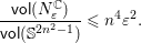
The same ideas allow one to derive bounds for the tail and expectation of the condition number of complex matrices. The set  $N_{{\it\varepsilon}}^{\mathbb{C}}$ is defined as in the real case, and one can prove that
 $$\begin{eqnarray}\frac{\mathsf{vol}(N_{{\it\varepsilon}}^{\mathbb{C}})}{\mathsf{vol}(\mathbb{S}^{2n^{2}-1})}\leq n^{4}{\it\varepsilon}^{2}.\end{eqnarray}$$
The following result for the set  ${\mathcal{M}}_{n}^{\mathbb{C}}$ of complex
 $n\times n$ matrices is an easy corollary of this bound.
Theorem 3.10. The probability that  ${\it\mu}(A)>1/{\it\varepsilon}$ or that
 ${\it\kappa}(A)>1/{\it\varepsilon}$ for either the standard Gaussian probability distribution on
 ${\mathcal{M}}_{n}^{\mathbb{C}}$ or the uniform distribution on
 $\mathbb{S}^{2n^{2}-1}$ (the unit sphere in
 ${\mathcal{M}}_{n}^{\mathbb{C}}$) is less than or equal to
 $n^{4}{\it\varepsilon}^{2}$. Also,
 $$\begin{eqnarray}\underset{A\sim N_{\mathbb{C}}(0,\text{Id})}{\mathbb{E}}\log {\it\kappa}(A)\leq 2\log n+O(1).\end{eqnarray}$$
(e) Average loss of precision in linear equation solving.
The bound in (3.4) and Theorem 3.9 immediately yield the following result on the expected loss of precision in linear equation solving.
Theorem 3.11. For all  $b\in \mathbb{R}^{n}$,
 $$\begin{eqnarray}\mathbb{E}_{A\sim N(0,\text{Id})}\mathsf{LoP}(A,b)\leq 5\log n+O(1).\square\end{eqnarray}$$
(f) Additional results.
The condition number  ${\it\kappa}$ is doubtless better studied than any other condition number. Because of this, the content of the previous pages is just a small fraction of what is known about them. Without intending to fill this gap entirely, we next state two results that either sharpen or add to this content.
The first, by Alan Edelman (Reference Edelman1988), shows a sharp bound for  $\mathbb{E}\log {\it\kappa}(A)$.
Theorem 3.12. For both real and complex standard Gaussian  $n\times n$ matrices
 $A$ we have
 $$\begin{eqnarray}\mathbb{E}\log {\it\kappa}(A)=\log n+C+O(1),\end{eqnarray}$$
where  $C=1.537$ in the real case and
 $C=0.982$ in the complex case. ◻
The second one is the best smoothed analysis, as of today, for  ${\it\kappa}(A)$. It is due to Mario Wschebor (Reference Wschebor2004).
Theorem 3.13. There exists a universal constant  $K\geq 1$ such that for all
 $\overline{A}\in \mathbb{R}^{n\times n}$ with
 $\Vert \overline{A}\Vert \leq 1$, all
 $0<{\it\sigma}\leq 1$, and all
 $t\geq 1$, we have
 $$\begin{eqnarray}\underset{A\sim N(\overline{A},{\it\sigma}^{2}\text{Id})}{\mathsf{Prob}}\{{\it\kappa}(A)\geq t\}\leq Kn\,\frac{1}{{\it\sigma}t}.\end{eqnarray}$$
Consequently, for all  ${\it\sigma}\in (0,1]$ and all
 $\overline{A}\in \mathbb{R}^{n\times n}$ with
 $\Vert \overline{A}\Vert \leq 1$, we have
 $$\begin{eqnarray}\mathbb{E}_{A\sim N(\overline{A},{\it\sigma}^{2}\text{Id})}(\log {\it\kappa}(A))\leq \log n+\log \frac{1}{{\it\sigma}}+2+\log K.\square\end{eqnarray}$$
3.2 Triangular linear systems
Theorem 3.11 shows that the expected loss of precision in the solution of linear systems is logarithmic in the dimension of the system. This is a reassuring result which appears to tally with computational practice.
In contrast, the solution of triangular systems of linear equations has puzzled practitioners for decades. They have long observed that these systems are generally solved to high accuracy in spite of being, in general, ill-conditioned. Thus, for instance, J. H. Wilkinson (Reference Wilkinson1963, p. 105): ‘In practice one almost invariably finds that if  $L$ is ill-conditioned, so that
 $\Vert L\Vert \Vert L^{-1}\Vert \gg 1$, then the computed solution of
 $Lx=b$ (or the computed inverse) is far more accurate than [forward stability analysis] would suggest.’
The statement that in general, triangular linear systems are poorly conditioned, was given a precise meaning by Viswanath and Trefethen (Reference Viswanath and Trefethen1998). They showed that, if  $L_{n}$ denotes a random lower triangular
 $n\times n$ matrix (with the entries in the diagonal and below independently distributed and drawn from
 $N(0,1)$), then
 $$\begin{eqnarray}\sqrt[n]{{\it\kappa}(L_{n})}\rightarrow 2\quad \text{almost surely}\end{eqnarray}$$
as  $n\rightarrow \infty$. It follows from this result that
 $\mathbb{E}(\log {\it\kappa}(L))={\rm\Omega}(n)$, a result that suggests an expected loss of precision linear in
 $n$. Were computational practice to conform to this bound, we would not be able to accurately solve triangular linear systems. But in practice, on almost every occasion, the accuracy of the computed solution is very high. It seems there is a gap between computing practice and theoretical predictions (at least so long as random matrices are modelled with a Gaussian distribution).
Nicholas Higham (Reference Higham1989) pointed out that the backward error analysis given by Wilkinson (Reference Wilkinson1963, Ch. 3, § 19) for forward substitution yields (small) componentwise bounds on the perturbed matrix (see also Bürgisser and Cucker Reference Bürgisser and Cucker2013, Proposition 3.5).
Proposition 3.14. Let  $L=(l_{ij})\in \mathbb{R}^{n\times n}$ be a non-singular triangular matrix,
 $b\in \mathbb{R}^{n}$, and assume
 ${\it\epsilon}_{\mathsf{mach}}$ is sufficiently small (of the order of
 $(\log n)^{-1}$). Then, the solution
 $\hat{x}$ of the system
 $Lx=b$ computed using forward substitution satisfies
 $$\begin{eqnarray}(L+E)\hat{x}=b,\end{eqnarray}$$
for some matrix  $E=(e_{ij})\in \mathbb{R}^{n\times n}$ with
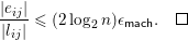 $$\begin{eqnarray}\frac{|e_{ij}|}{|l_{ij}|}\leq (2\log _{2}n){\it\epsilon}_{\mathsf{mach}}.\square\end{eqnarray}$$
An argument similar to that used to derive (3.3), with Proposition 3.14 replacing Theorem 3.1, allows us to prove
 $$\begin{eqnarray}\max _{i\leq n}\frac{|\tilde{x}_{i}-x_{i}|}{|x_{i}|}\leq 2\log _{2}(n)\,{\it\epsilon}_{\mathsf{mach}}\mathsf{Cw}^{{\it\varphi}}(L,b)+o({\it\epsilon}_{\mathsf{mach}}),\end{eqnarray}$$
where  $\mathsf{Cw}^{{\it\varphi}}(L,b)$ is the componentwise condition number given by (1.3) with
 $$\begin{eqnarray}\mathsf{RelError}(\tilde{L},\tilde{b}):=\max _{\substack{ 1\leq i\leq j\leq n \\ 1\leq \ell \leq n}}\biggl\{\frac{|\tilde{l}_{ij}-l_{ij}|}{|l_{ij}|},\frac{|\tilde{b}_{\ell }-b_{\ell }|}{|b_{\ell }|}\biggr\}.\end{eqnarray}$$
Consequently, the loss of precision in solving triangular systems is bounded by
 $$\begin{eqnarray}\mathsf{LoP}(L^{-1}b)\leq \log (\log _{2}n)+\log \mathsf{Cw}^{{\it\varphi}}(L,b)+\log 2+o(1).\end{eqnarray}$$
As in Section 3.1, we want to trade the occurrence of  $\log \mathsf{Cw}^{{\it\varphi}}(L,b)$ in exchange for some probabilistic uncertainty. The next result (Theorem 1.1 in Cheung and Cucker Reference Cheung and Cucker2015) does this. For a matrix
 $A$ we define the max norm
 $$\begin{eqnarray}\Vert A\Vert _{\max }:=\max _{ij}|a_{ij}|.\end{eqnarray}$$
Theorem 3.15. Let  ${\mathcal{T}}$ denote the set of
 $n\times n$ lower triangular matrices. Let
 $\bar{L}\in {\mathcal{T}}$ and
 $\bar{b}\in \mathbb{R}^{n}$ be such that
 $\Vert \bar{L}\Vert _{\max }\leq 1$ and
 $\Vert \bar{b}\Vert _{\infty }\leq 1$. For
 $L\in {\mathcal{T}}$ and
 $b\in \mathbb{R}^{n}$ let
 $\mathsf{Cw}(L,b)$ denote the componentwise condition number, for the problem of linear equation solving, of the pair
 $(L,b)$. Then, for any real number
 $t>n(n+1)$ we have
 $$\begin{eqnarray}\mathsf{Prob}_{(L,b)\sim N_{{\mathcal{T}}}((\bar{L},\bar{b}),{\it\sigma}^{2}\text{Id})}\{\mathsf{Cw}(L,b)>t\}\leq \biggl(\frac{1+{\it\sigma}}{{\it\sigma}}\biggr)\biggl(\frac{n^{3}(n+1)^{2}}{t-n(n+1)}\biggr)\sqrt{\frac{2}{{\it\pi}}}\end{eqnarray}$$
and
 $$\begin{eqnarray}\mathbb{E}_{(L,b)\sim N_{{\mathcal{T}}}((\bar{L},\bar{b}),{\it\sigma}^{2}\text{Id})}(\log (\mathsf{Cw}(L,b)))\leq \log \biggl(\frac{1+{\it\sigma}}{{\it\sigma}}\biggr)+5\log (n)+1.16.\end{eqnarray}$$
The subindex  ${\mathcal{T}}$ in
 $N_{{\mathcal{T}}}((\bar{L},\bar{b}),{\it\sigma}^{2}\text{Id})$ is meant to denote that
 $L$ is triangular. That is, the only entries of
 $L$ which are drawn from the Gaussian
 $N((\bar{L},\bar{b}),{\it\sigma}^{2}\text{Id})$ are those in its lower part. ◻
Note that if we replace  $(L,b)$ with
 $(cL,cb)$ we obtain the same
 $\mathsf{Cw}$. That is,
 $\mathsf{Cw}(L,b)=\mathsf{Cw}(cL,cb)$. Indeed, the relative errors will be the same for both pairs. The bounds on the norms of
 $\bar{L}$ and
 $\bar{b}$ are, as usual, to give some feel for the magnitude of
 ${\it\sigma}$.
Theorem 3.15 together with (3.11) provides a smoothed analysis for the loss of precision for the solution of linear triangular systems via forward substitution.
Corollary 3.16. Assume we solve systems  $Lx=b$ using forward substitution. Then, for all
 $\bar{L}\in {\mathcal{T}}$ and
 $\bar{b}\in \mathbb{R}^{n}$ with
 $\Vert \bar{L}\Vert _{\max }\leq 1$ and
 $\Vert \bar{b}\Vert _{\infty }\leq 1$ we have
 $$\begin{eqnarray}\mathbb{E}(\mathsf{LoP}(x))\leq \log \biggl(\frac{1+{\it\sigma}}{{\it\sigma}}\biggr)+5\log n+\log (\log _{2}n)+1.452+o(1).\end{eqnarray}$$
Here  $x=L^{-1}b$ with
 $(L,b)\sim N_{{\mathcal{T}}}((\bar{L},\bar{b}),{\it\sigma}^{2}\text{Id})$ and
 $o(1)$ is a quantity that tends to zero with
 ${\it\epsilon}_{\mathsf{mach}}$.◻
3.3 Linear least-squares
A way of dealing with overdetermined linear systems going back to Gauss is to compute for them a point minimizing the residual. More precisely, for a rectangular matrix  $R\in \mathbb{R}^{q\times n}$ with
 $q>n$ and a point
 $c\in \mathbb{R}^{q}$, one computes
 $$\begin{eqnarray}x:=\arg \min _{v\in \mathbb{R}^{n}}\Vert Rv-c\Vert .\end{eqnarray}$$
This point  $x$ is given by
 $R^{\dagger }c$ where
 $R^{\dagger }$ is the Moore–Penrose inverse of
 $R$ which, when
 $R$ is full-rank, satisfies
 $R^{\dagger }=(R^{\text{T}}R)^{-1}R^{\text{T}}$. To actually compute
 $x$, QR factorization again turns out to be of help. Indeed, Theorem 3.1 is a special case of a more general result (Theorem 19.3 of Higham Reference Higham1996), which we now quote in full.
Theorem 3.17. Let  $R\in \mathbb{R}^{q\times n}$ have full rank,
 $q\geq n$,
 $c\in \mathbb{R}^{q}$, and suppose that the least-squares problem
 $\arg \min _{v}\Vert c-Rv\Vert$ is solved using the Householder QR factorization method. The computed solution
 $\tilde{x}$ is the exact solution to
 $$\begin{eqnarray}\arg \min _{v\in \mathbb{R}^{n}}\Vert \tilde{c}-\tilde{R}v\Vert ,\end{eqnarray}$$
where  $\tilde{R}$ and
 $\tilde{c}$ satisfy the relative error bounds
 $$\begin{eqnarray}\Vert \tilde{R}-R\Vert _{F}\leq n{\it\gamma}_{cq}\Vert R\Vert _{F}\quad \text{and}\quad \Vert \tilde{c}-c\Vert \leq n{\it\gamma}_{sq}\Vert c\Vert\end{eqnarray}$$
for a small constant  $s$.◻
Reasoning as in Section 3.1, we see that the loss of precision in the computation of  $x$ is bounded by
 $$\begin{eqnarray}\mathsf{LoP}(R^{\dagger }c)\leq \log (n^{3/2}q)+\log \mathsf{cond}^{\dagger }(R,c)+\log s+o(1),\end{eqnarray}$$
where  $\mathsf{cond}(R,c)$ is the normwise condition number for linear least-squares (with respect to the spectral norm). That is,
 $$\begin{eqnarray}\mathsf{cond}^{\dagger }(R,c):=\lim _{{\it\delta}\rightarrow 0}\sup _{\max \{\mathsf{RelError}(\tilde{R}),\mathsf{RelError}(\tilde{c})\}\leq {\it\delta}}\frac{\mathsf{RelError}(\tilde{x})}{{\it\delta}},\end{eqnarray}$$
where
 $$\begin{eqnarray}\mathsf{RelError}(\tilde{x}):=\frac{\Vert x-\tilde{x}\Vert }{\Vert x\Vert }\end{eqnarray}$$
and similarly for  $\mathsf{RelError}(\tilde{R})$ and
 $\mathsf{RelError}(\tilde{c})$. If, following (3.5), we define
 $$\begin{eqnarray}{\it\kappa}_{\dagger }(R):=\Vert R\Vert \Vert R^{\dagger }\Vert ,\end{eqnarray}$$
we can prove that  $\mathsf{cond}^{\dagger }(R,c)$, even though not tightly approximated by
 ${\it\kappa}_{\dagger }(R)$, is bounded by a constant times
 ${\it\kappa}_{\dagger }^{2}(R)$ (see Wedin Reference Wedin1973). Consequently, to obtain expected bounds (or a smoothed analysis) for the loss of precision
 $\mathsf{LoP}(R^{\dagger }c)$ from equation (3.12), it is enough to perform the corresponding analysis for
 $\log {\it\kappa}_{\dagger }(R)$. The following result (Theorem 4.2 in Bürgisser and Cucker Reference Bürgisser and Cucker2013) exhibits a smoothed analysis for
 ${\it\kappa}_{\dagger }(R)$.
Theorem 3.18. For all  ${\it\lambda}_{0}\in (0,1)$ there exists
 $q_{0}$ such that for all
 $1\leq n\leq q$ with
 ${\it\lambda}=(n-1)/q\leq {\it\lambda}_{0}$ and
 $q\geq q_{0}$, we have for all
 ${\it\sigma}$ with
 $1/\sqrt{n}\leq {\it\sigma}\leq 1$ and all
 $\overline{R}\in \mathbb{R}^{q\times n}$ with
 $\Vert \overline{R}\Vert \leq 1$, that
 $$\begin{eqnarray}\mathbb{E}_{R\sim N(\overline{R},{\it\sigma}^{2}\text{Id})}({\it\kappa}_{\dagger }(R))\leq \frac{20.1}{1-{\it\lambda}}.\square\end{eqnarray}$$
Jensen’s inequality immediately yields the following consequence.
Corollary 3.19. Under the hypothesis of Theorem 3.18,
 $$\begin{eqnarray}\sup _{\Vert \overline{R}\Vert \leq 1}\mathbb{E}_{R\sim N(\overline{R},{\it\sigma}^{2}\text{Id})}(\log {\it\kappa}_{\dagger }(R))\leq \log \biggl(\frac{20.1}{1-{\it\lambda}}\biggr).\square\end{eqnarray}$$
It is worth noting that the bounds in Theorem 3.18 and Corollary 3.19 are independent of  $q$ and
 $n$, as long as
 $q$ is sufficiently large and the elongation
 ${\it\lambda}$ is sufficiently small. But they depend only on
 ${\it\lambda}$. Indeed, perhaps surprisingly, they are even independent of
 ${\it\sigma}$. In fact, Corollary 3.19 indicates that for large, reasonably elongated matrices, one may expect the loss of precision in the solution of least-squares problems to derive mostly from the backward error bounds of the algorithm used (e.g. QR factorization).
3.4 The conjugate gradient method
In the preceding paragraph we saw that the solution  $x\in \mathbb{R}^{n}$ of the problem
 $$\begin{eqnarray}x:=\arg \min _{v\in \mathbb{R}^{n}}\Vert Rv-c\Vert ,\end{eqnarray}$$
when  $R\in \mathbb{R}^{q\times n}$ is full-rank, is given by
 $$\begin{eqnarray}x=R^{\dagger }c=(R^{\text{T}}R)^{-1}R^{\text{T}}c.\end{eqnarray}$$
It follows that we can find  $x$ as the solution of the system
 $Ax=b$ with
 $A:=R^{\text{T}}R$,
 $A\in \mathbb{R}^{n\times n}$, and
 $b:=R^{\text{T}}c$.
Now, by construction,  $A$ is symmetric and positive definite. One may therefore consider algorithms exploiting symmetry and positive definiteness.
Notable among the algorithms doing so is the conjugate gradient method. In what follows we briefly describe how this algorithm works, how its convergence rate is controlled by the condition number  ${\it\kappa}(A)$, and how probabilistic analyses of the latter yield probabilistic estimates on the complexity of the conjugate gradient. The role played by
 ${\it\kappa}(A)$ in this development regards the complexity of an algorithm rather than its numerical stability. To better focus on this role, we will disregard all issues concerning finite precision and assume, instead, infinite precision in all computations.
(a) The algorithm.
For  $x\in \mathbb{R}^{n}$ we define its
 $A$-norm by
 $$\begin{eqnarray}\Vert x\Vert _{A}:=(x^{\text{T}}Ax)^{1/2}\end{eqnarray}$$
coming from the scalar product
 $$\begin{eqnarray}\left\langle x,y\right\rangle _{A}:=x^{\text{T}}Ay.\end{eqnarray}$$
We say that  $x,y$ are
 $A$-orthogonal (or conjugated) if
 $\left\langle x,y\right\rangle _{A}=0$. Let
 $(d_{0},\ldots ,d_{n-1})$ be an
 $A$-orthogonal basis of
 $\mathbb{R}^{n}$, that is,
 $\left\langle d_{i},d_{j}\right\rangle _{A}=0$ for
 $i\neq j$. Moreover, let
 $\bar{x}$ be the solution of
 $Ax=b$ and
 $x_{0}\in \mathbb{R}^{n}$ be an initial point. Expand
 $$\begin{eqnarray}\bar{x}-x_{0}=\mathop{\sum }_{i=0}^{n-1}{\it\alpha}_{i}d_{i},\end{eqnarray}$$
with  ${\it\alpha}_{i}\in \mathbb{R}$. Then, by
 $A$-orthogonality,
 $$\begin{eqnarray}{\it\alpha}_{k}=\frac{\left\langle \bar{x}-x_{0},d_{k}\right\rangle _{A}}{\Vert d_{k}\Vert _{A}^{2}}.\end{eqnarray}$$
Define
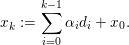 $$\begin{eqnarray}x_{k}:=\mathop{\sum }_{i=0}^{k-1}{\it\alpha}_{i}d_{i}+x_{0}.\end{eqnarray}$$
Then we have  $\left\langle x_{k}-x_{0},d_{\ell }\right\rangle _{A}=0$, for all
 $\ell =k,\ldots ,n-1$. In particular, taking
 $\ell =k$,
 $$\begin{eqnarray}\left\langle \bar{x}-x_{0},d_{k}\right\rangle _{A}=\left\langle \bar{x}-x_{k},d_{k}\right\rangle _{A}=d_{k}^{\text{T}}A(\bar{x}-x_{k})=d_{k}^{\text{T}}r_{k},\end{eqnarray}$$
with the residue  $r_{k}:=b-Ax_{k}=A\bar{x}-Ax_{k}$. We obtain that
 $$\begin{eqnarray}{\it\alpha}_{k}=\frac{\left\langle d_{k},r_{k}\right\rangle }{\Vert d_{k}\Vert _{A}^{2}}.\end{eqnarray}$$
Note that  ${\it\alpha}_{k}$ depends only on
 $d_{k}$ and
 $r_{k}$.
(a) For
$k\geq 1$, $x_{k}$ minimizes the function $x\mapsto \Vert x-\bar{x}\Vert _{A}$ on the line $x_{k-1}+\mathbb{R}d_{k-1}$ as well as on the affine space $x_{0}+\mathsf{span}\{d_{0},\ldots ,d_{k-1}\}$.(b) We have
$\left\langle r_{k},d_{i}\right\rangle =0$ for $i<k$. In particular, $r_{n}=0$ and $x_{n}=\bar{x}$.





Proof. For part (a) note that the point  $x_{k}-x_{0}$ is the
 $A$-orthogonal projection of
 $\bar{x}-x_{0}$ onto
 $\mathsf{span}\{d_{0},\ldots ,d_{k-1}\}$. Therefore,
 $x_{k}-x_{0}$ minimizes the
 $A$-distance to
 $\bar{x}$,
 $$\begin{eqnarray}x\;\mapsto \;\Vert x-\bar{x}\Vert _{A}=\Vert (x-x_{0})-(\bar{x}-x_{0})\Vert _{A},\end{eqnarray}$$
on  $x_{0}+\mathsf{span}\{d_{0},\ldots ,d_{k-1}\}$.
For part (b), consider the function
 $$\begin{eqnarray}f(x):=\frac{1}{2}x^{\text{T}}Ax-b^{\text{T}}x.\end{eqnarray}$$
The gradient of  $f$ at
 $x$ is
 $\mathsf{grad}\,f(x)=Ax-b$, and it is easy to see (Bürgisser and Cucker Reference Bürgisser and Cucker2013, § 5.2) that
 $$\begin{eqnarray}f(x)=\frac{1}{2}\Vert x-\bar{x}\Vert _{A}^{2}+f(\bar{x}).\end{eqnarray}$$
Part (a) then implies that  $x_{k}$ minimizes
 $f$ on
 $x_{0}+\mathsf{span}\{d_{0},\ldots ,d_{k-1}\}$. Hence,
 $\mathsf{grad}\,f(x_{k})$ is orthogonal to
 $\mathsf{span}\{d_{0},\ldots ,d_{k-1}\}$. But
 $\mathsf{grad}\,f(x_{k})=-r_{k}$, which proves the first statement in (b). The second statement follows from the fact that
 $r_{n}$ is then orthogonal to
 $d_{0},\ldots ,d_{n-1}$ (and hence it must be 0). This, in turn, implies
 $x_{n}=\bar{x}$.
Thus far, we have assumed an  $A$-orthogonal basis
 $\{d_{0},\ldots ,d_{n-1}\}$ at hand. The conjugate gradient method actually computes one, along with the computation of the
 $x_{k}$, by sequentially choosing the directions
 $d_{k}$ as conjugates of the gradients
 $-r_{k}$. Algorithm 1 shows how this is done (a proof of the
 $A$-orthogonality of the resulting set can be found in Bürgisser and Cucker Reference Bürgisser and Cucker2013, Theorem 5.12).

(b) First complexity considerations.
We begin by looking at the cost (i.e. number of arithmetic operations performed) of each iteration of the algorithm. The cost of computing an inner product, such as  $\langle r_{k},d_{k}\rangle$, is
 $2n-1$. Consequently, the cost of a matrix–vector multiplication, such as
 $Ax_{k}$, is
 $2n^{2}-n$. It follows that computing an
 $A$-inner product costs
 $2n^{2}+n-1$. At each iteration of Conj_Grad the computation of each of
 $x_{k+1}$ and
 $d_{k+1}$ thus takes
 $O(n)$ arithmetic operations, and those of
 ${\it\alpha}_{k}$,
 $r_{k+1}$, and
 ${\it\beta}_{k}$ take
 $2n^{2}+O(n)$ each (note that for the latter we use the already computed
 $\Vert d_{k}\Vert _{A}^{2}$). That is, the cost of an iteration of Conj_Grad is
 $6n^{2}+O(n)$.
It follows from this bound that the cost of computing the solution  $\bar{x}$ of
 $Ax=b$ is
 $6n^{3}+O(n^{2})$. This bound is larger than the
 $\frac{2}{3}n^{3}$ bound for the cost of Gaussian elimination, making the conjugate gradient a poor choice for the computation of
 $\bar{x}$.
We note at this juncture, however, that unlike Gaussian elimination, the conjugate gradient produces a sequence  $x_{k}$ of approximations of
 $\bar{x}$. If we are only interested in a good approximation, as opposed to the exact value of
 $\bar{x}$, then early termination of the conjugate gradient might outperform Gaussian elimination. To understand this issue we need to estimate the speed of convergence of the former.
(c) Convergence analysis.
Let  ${\it\epsilon}_{k}:=x_{k}-\bar{x}$ be the
 $k$th error.
Theorem 3.21. The error at the  $k$th step of the conjugate gradient satisfies
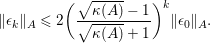 $$\begin{eqnarray}\Vert {\it\epsilon}_{k}\Vert _{A}\leq 2\biggl(\frac{\sqrt{{\it\kappa}(A)}-1}{\sqrt{{\it\kappa}(A)}+1}\biggr)^{k}\Vert {\it\epsilon}_{0}\Vert _{A}.\end{eqnarray}$$
Corollary 3.22. For all  ${\it\delta}>0$ we have
 $\Vert {\it\epsilon}_{k}\Vert _{A}\leq {\it\delta}\Vert {\it\epsilon}_{0}\Vert _{A}$ whenever
 $$\begin{eqnarray}k\geq \ln \biggl(\frac{\sqrt{{\it\kappa}(A)}+1}{\sqrt{{\it\kappa}(A)}-1}\biggr)^{-1}\ln \biggl(\frac{2}{{\it\delta}}\biggr)\approx \frac{1}{2}\sqrt{{\it\kappa}(A)}\ln \biggl(\frac{1}{{\it\delta}}\biggr).\end{eqnarray}$$
With the proof of Theorem 3.21 in mind, we introduce some notation. We  ${\mathcal{P}}_{k}$ denote the linear space of all real polynomials in one variable
 $X$ with degree at most
 $k$. We also write
 ${\mathcal{Q}}_{k}$ for the subset of
 ${\mathcal{P}}_{k}$ of polynomials with constant coefficient 1.
Theorem 3.23. The error  ${\it\epsilon}_{k}$ at the
 $k$th step of the conjugate gradient method satisfies
 $$\begin{eqnarray}\Vert {\it\epsilon}_{k}\Vert _{A}^{2}\leq \min _{q\in {\mathcal{Q}}_{k}}\max _{j\leq n}q({\it\lambda}_{j})^{2}\cdot \Vert {\it\epsilon}_{0}\Vert _{A}^{2},\end{eqnarray}$$
where  ${\it\lambda}_{1},\ldots ,{\it\lambda}_{n}$ are the eigenvalues of
 $A$.
Proof. By Proposition 3.20(a) we know that  $x_{k}$ minimizes the
 $A$-distance of
 $\bar{x}$ to the affine space
 $$\begin{eqnarray}x_{0}+S_{k-1}=x_{0}+\mathsf{span}\{d_{0},\ldots ,d_{k-1}\}=x_{0}+\mathsf{span}\{r_{0},Ar_{0},\ldots ,A^{k-1}r_{0}\}.\end{eqnarray}$$
An element  $x$ of
 $x_{0}+S_{k-1}$ can therefore be written as
 $$\begin{eqnarray}x=x_{0}-p(A)r_{0},\end{eqnarray}$$
with  $p\in {\mathcal{P}}_{k-1}$, and conversely, for any such polynomial we obtain
 $x\in x_{0}+Sk-1$. Using
 $r_{0}=b-Ax_{0}=A(\bar{x}-x_{0})$ we get
 $$\begin{eqnarray}\displaystyle x-\bar{x} & = & \displaystyle x_{0}-\bar{x}-p(A)A(\bar{x}-x_{0})=x_{0}-\bar{x}+Ap(A)(x_{0}-\bar{x})\nonumber\\ \displaystyle & = & \displaystyle (\text{Id}+Ap(A))(x_{0}-\bar{x}).\nonumber\end{eqnarray}$$
It follows that the error  ${\it\epsilon}_{k}=x_{k}-\bar{x}$ at the
 $k$th step of the conjugate gradient method satisfies
 $$\begin{eqnarray}\Vert {\it\epsilon}_{k}\Vert _{A}=\min _{x\in x_{0}+S_{k-1}}\Vert x-\bar{x}\Vert _{A}=\min _{p\in {\mathcal{P}}_{k-1}}\Vert (\text{Id}+Ap(A)){\it\epsilon}_{0}\Vert _{A}.\end{eqnarray}$$
Suppose that  $v_{1},\ldots ,v_{n}$ is an orthonormal basis of eigenvectors of
 $A$ corresponding to the eigenvalues
 ${\it\lambda}_{1}\geq \cdots \geq {\it\lambda}_{n}>0$. Write
 $$\begin{eqnarray}{\it\epsilon}_{0}=x_{0}-\bar{x}=\mathop{\sum }_{j=1}^{n}{\it\xi}_{j}v_{j}\end{eqnarray}$$
for some  ${\it\xi}_{1},\ldots ,{\it\xi}_{n}\in \mathbb{R}$. Then
 $$\begin{eqnarray}\Vert {\it\epsilon}_{0}\Vert _{A}^{2}=\mathop{\sum }_{j=1}^{n}\mathop{\sum }_{k=1}^{n}{\it\xi}_{j}{\it\xi}_{k}\;v_{j}^{\text{T}}Av_{k}=\mathop{\sum }_{j=1}^{n}{\it\lambda}_{j}{\it\xi}_{j}^{2}.\end{eqnarray}$$
Moreover, for any polynomial  $p\in {\mathcal{P}}_{k-1}$,
 $$\begin{eqnarray}(\text{Id}+Ap(A)){\it\epsilon}_{0}=\mathop{\sum }_{j=1}^{n}(1+{\it\lambda}_{j}p({\it\lambda}_{j})){\it\xi}_{j}v_{j}.\end{eqnarray}$$
Therefore
 $$\begin{eqnarray}\Vert (\text{Id}+Ap(A)){\it\epsilon}_{0}\Vert _{A}^{2}=\mathop{\sum }_{j=1}^{n}(1+{\it\lambda}_{j}p({\it\lambda}_{j}))^{2}{\it\lambda}_{j}{\it\xi}_{j}^{2}\leq \max _{j\leq n}(1+{\it\lambda}_{j}p({\it\lambda}_{j}))^{2}\mathop{\sum }_{j=1}^{n}{\it\lambda}_{j}{\it\xi}_{j}^{2},\end{eqnarray}$$
and using (3.14),
 $$\begin{eqnarray}\Vert {\it\epsilon}_{k}\Vert _{A}^{2}\leq \min _{p\in {\mathcal{P}}_{k-1}}\max _{j\leq n}(1+{\it\lambda}_{j}p({\it\lambda}_{j}))^{2}\mathop{\sum }_{j=1}^{n}{\it\lambda}_{j}{\it\xi}_{j}^{2}.\end{eqnarray}$$
The result now follows by observing that  ${\mathcal{Q}}_{k}=1+X{\mathcal{P}}_{k-1}$.
Theorem 3.23 is hard to apply in concrete situations. It depends on all the eigenvalues of  $A$ and it optimizes a function of them over the space
 ${\mathcal{Q}}_{k}$. It is nevertheless a building block in the proof of Theorem 3.21. We proceed to see why.
Suppose that  ${\it\lambda}_{n}=a$ and
 ${\it\lambda}_{1}=b$, for
 $0<a<b$. What are the optimal polynomials
 $q\in {\mathcal{Q}}_{k}$ if nothing is known about the location of the eigenvalues
 ${\it\lambda}$ except that
 ${\it\lambda}\in [a,b]$? In this case we have to minimize the quantity
 $$\begin{eqnarray}\max _{a\leq {\it\lambda}\leq b}q({\it\lambda})^{2}\end{eqnarray}$$
over all real polynomials  $q\in {\mathcal{Q}}_{k}$. This minimization problem can also be considered for arbitrary
 $a,b\in \mathbb{R}$ with
 $a<b$. In the particular case
 $a=-1$,
 $b=1$ it turns out that its solution is given by the Chebyshev polynomials
 $T_{k}$ (defined by the equation
 $\cos (k{\it\phi})=T_{k}(\cos ({\it\phi}))$).
Proposition 3.24. For all  $0<a<b$ we have
 $$\begin{eqnarray}\min _{\substack{ \mathsf{deg}q\leq k \\ q(0)=1}}\;\max _{a\leq {\it\lambda}\leq b}q({\it\lambda})^{2}=\frac{1}{T_{k}(\frac{b+a}{b-a})^{2}}.\end{eqnarray}$$
Proof. The polynomial
 $$\begin{eqnarray}p({\it\lambda}):=\frac{T_{k}(\frac{b+a-2{\it\lambda}}{b-a})}{T_{k}(\frac{b+a}{b-a})}\end{eqnarray}$$
has degree  $k$, satisfies
 $p(0)=1$, and
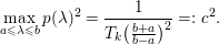 $$\begin{eqnarray}\max _{a\leq {\it\lambda}\leq b}p({\it\lambda})^{2}=\frac{1}{T_{k}(\frac{b+a}{b-a})^{2}}=:c^{2}.\end{eqnarray}$$
(Note that  ${\it\lambda}\mapsto (b+a-2{\it\lambda})/(b-a)$ maps
 $[a,b]$ onto
 $[-1,1]$ and
 $T_{k}$ has maximal value 1 on this interval.)
In order to show the optimality of  $p$, suppose that for some polynomial
 $q\in {\mathcal{Q}}_{k}$,
 $$\begin{eqnarray}\max _{a\leq {\it\lambda}\leq b}|q({\it\lambda})|<\max _{a\leq {\it\lambda}\leq b}|p({\it\lambda})|.\end{eqnarray}$$
Since  $p$ alternately takes the values
 $c,-c,c,-c,\ldots$ exactly
 $k+1$ times in the interval
 $[a,b]$, we conclude that the polynomial
 $p-q$ has at least
 $k$ roots in this interval (intermediate value theorem). Moreover,
 $p(0)-q(0)=1-1=0$. Hence
 $p-q$ has degree at most
 $k$ and
 $k+1$ distinct roots. It follows that
 $p=q$.
Proof of Theorem 3.21.
To estimate the optimal value in Proposition 3.24, note that for  $z\in \mathbb{C}$,
 $z=\cos ({\it\phi})+i\sin ({\it\phi})=x+i\sqrt{1-x^{2}}$, we have
 $$\begin{eqnarray}T_{k}(x)=\mathsf{Re}(z^{k})=\frac{1}{2}(z^{k}+\overline{z}^{k})=\frac{1}{2}((x+\sqrt{x^{2}-1})^{k}+(x-\sqrt{x^{2}-1})^{k}).\end{eqnarray}$$
Again take  $a={\it\lambda}_{n}$,
 $b={\it\lambda}_{1}$, the smallest and largest eigenvalues of
 $A$. Then
 ${\it\kappa}={\it\kappa}(A)=b/a$. For
 $$\begin{eqnarray}x=\frac{b+a}{b-a}=\frac{{\it\kappa}+1}{{\it\kappa}-1}\end{eqnarray}$$
we get
 $$\begin{eqnarray}x^{2}-1=\frac{({\it\kappa}+1)^{2}-({\it\kappa}-1)^{2}}{({\it\kappa}-1)^{2}}=\frac{4{\it\kappa}}{({\it\kappa}-1)^{2}}\end{eqnarray}$$
and therefore
 $$\begin{eqnarray}x+\sqrt{x^{2}-1}=\frac{{\it\kappa}+1+2\sqrt{{\it\kappa}}}{{\it\kappa}-1}=\frac{(\sqrt{{\it\kappa}}+1)^{2}}{{\it\kappa}-1}=\frac{\sqrt{{\it\kappa}}+1}{\sqrt{{\it\kappa}}-1}.\end{eqnarray}$$
Hence
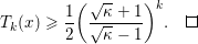 $$\begin{eqnarray}T_{k}(x)\geq \frac{1}{2}\biggl(\frac{\sqrt{{\it\kappa}}+1}{\sqrt{{\it\kappa}}-1}\biggr)^{k}.\square\end{eqnarray}$$
(d) Conjugate gradient on random data.
Theorem 3.21 gives bounds for the rate of convergence of the conjugate gradient in terms of the condition  ${\it\kappa}(A)$ of the matrix
 $A$. An average (or smoothed) analysis of
 ${\it\kappa}(A)$ would therefore result in an average (resp. smoothed) analysis for this rate of convergence. The question that emerges is which probability distribution we draw
 $A$ from.
In the case of unstructured or triangular matrices  $A$, we have endowed the corresponding class of matrices with a Gaussian distribution. In our present case, with
 $A$ positive definite, this choice is no longer available. A look at our original computational problem may, however, shed some light. Matrix
 $A$ is obtained as
 $A=R^{\text{T}}R$. It then makes sense to consider
 $R$ as our primary random data – and for
 $R$ we can assume Gaussianity – and endow
 $A$ with the distribution inherited from that of
 $R$. In the particular case that
 $R$ is standard Gaussian, this inherited distribution of
 $A$ is known as the Wishart distribution with
 $q$degrees of freedom. It extends the chi-square distribution, since it coincides with a
 ${\it\chi}_{q}^{2}$ when
 $n=1$.
By the Singular Value Decomposition, there exist orthogonal matrices  $U$ and
 $V$ and positive reals
 ${\it\sigma}_{1}\geq {\it\sigma}_{2}\geq \cdots \geq {\it\sigma}_{n}>0$ such that
 $R=U\mathsf{diag}({\it\sigma}_{1},{\it\sigma}_{2},\ldots ,{\it\sigma}_{n})V^{\text{T}}$. Then
 $$\begin{eqnarray}A=R^{\text{T}}R=V\mathsf{diag}({\it\sigma}_{1}^{2},{\it\sigma}_{2}^{2},\ldots ,{\it\sigma}_{n}^{2})V^{\text{T}}\end{eqnarray}$$
and, consequently,  ${\it\kappa}(A)={\it\kappa}_{\dagger }^{2}(R)$.
It follows from the above that the analysis of  ${\it\kappa}(A)$ for a Wishart distribution reduces to the analysis of
 ${\it\kappa}_{\dagger }(R)$ when
 $R$ is standard Gaussian (and similarly for ‘non-centred Wishart distributions’).
Corollary 3.22 shows that the number  $k$ of iterations needed to decrease
 $\Vert x_{0}-\bar{x}\Vert _{A}$ by a factor of
 ${\it\delta}$ is proportional to
 $\sqrt{{\it\kappa}(A)}$, that is, proportional to
 ${\it\kappa}_{\dagger }(R)$. Theorem 3.18 shows that for
 $q$ large enough and
 ${\it\lambda}=(n-1)/q$ small enough we have, for all
 $0<{\it\sigma}\leq 1$,
 $$\begin{eqnarray}\sup _{\Vert \overline{R}\Vert \leq 1}\mathbb{E}_{R\sim N(\overline{R},{\it\sigma}^{2}\text{Id})}({\it\kappa}_{\dagger }(R))\leq \frac{20.1}{1-{\it\lambda}}.\end{eqnarray}$$
Thus, if  $A$ is obtained as
 $R^{\text{T}}R$ for a large elongated rectangular matrix
 $R$, then we should expect to effect the decrease mentioned above with about
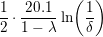 $$\begin{eqnarray}\frac{1}{2}\cdot \frac{20.1}{1-{\it\lambda}}\ln \biggl(\frac{1}{{\it\delta}}\biggr)\end{eqnarray}$$
iterations (where  ${\it\lambda}=q/n$ is the elongation). Since each iteration takes
 $6n^{2}+O(n)$ arithmetic operations, the expected cost of the computation is
 $$\begin{eqnarray}3n^{2}\frac{20.1}{1-{\it\lambda}}\ln \frac{1}{{\it\delta}}+O(n)=\frac{60.3n^{2}}{1-{\it\lambda}}\ln \frac{1}{{\it\delta}}+O(n).\end{eqnarray}$$
The leading term in this expression is smaller than the  $\frac{2}{3}n^{3}$ operations performed by Gaussian elimination as long as
 $$\begin{eqnarray}{\it\delta}\geq e^{-\frac{n(1-{\it\lambda})}{91}}.\end{eqnarray}$$
For large  $n$ (and
 ${\it\lambda}$ not too close to 1) this bound produces very small values of
 ${\it\delta}$, and therefore Conj_Grad yields, on average (both for a Gaussian distribution of data and for Gaussian perturbations of arbitrary data), remarkably good approximations of
 $\bar{x}$.
We conclude that for reasonable  ${\it\delta}>0$ and large
 $n$, computing an approximation of the solution
 $\bar{x}$ of
 $Ax=b$ using Algorithm Conj_Grad will typically be faster than computing
 $\bar{x}$ with Gaussian elimination.
3.5 Feasibility of polyhedral conic systems
(a) The feasibility problem and its condition.
A homogenization of the linear programming feasibility programme can be stated as follows. Given  $A\in \mathbb{R}^{m\times n}$,
 $n>m$, consider the primal feasibility problem

and the dual feasibility problem

We say that  $A$ is primal feasible or dual feasible when (PF) or (DF), respectively, is satisfied. In both cases we talk about strict feasibility when the satisfied inequality is strict.
Let  ${\mathcal{F}}_{P}$ and
 ${\mathcal{F}}_{D}$ denote the sets of matrices
 $A$ where (PF) and (DF) are satisfied, respectively, and let
 ${\mathcal{F}}_{P}^{\circ }$ and
 ${\mathcal{F}}_{D}^{\circ }$ be the sets of strictly primal and strictly dual feasible matrices. Finally, let
 $$\begin{eqnarray}{\rm\Sigma}:={\mathcal{F}}_{P}\cap {\mathcal{F}}_{D}.\end{eqnarray}$$
It is well known that, modulo a set of lower dimension, primal (dual) feasibility is equivalent to dual (resp. primal) strict infeasibility. The following result (see Bürgisser and Cucker Reference Bürgisser and Cucker2013, Theorem 6.14) is more precise. To state it, we let  $\mathsf{int}(M)$,
 $\overline{M}$, and
 $\partial M=\overline{M}\setminus \mathsf{int}(M)$ denote the interior, closure, and boundary of a subset
 $M$ of Euclidean space.
Theorem 3.25. Both  ${\mathcal{F}}_{P}$ and
 ${\mathcal{F}}_{D}$ are closed subsets of
 $\mathbb{R}^{m\times n}$. In addition, this space is partitioned as
 $$\begin{eqnarray}\mathbb{R}^{m\times n}=\mathsf{int}({\mathcal{F}}_{P}^{\circ })\cup \mathsf{int}({\mathcal{F}}_{D}^{\circ })\cup {\rm\Sigma},\end{eqnarray}$$
and we have
 $$\begin{eqnarray}{\rm\Sigma}=\partial {\mathcal{F}}_{P}=\partial {\mathcal{F}}_{D}.\end{eqnarray}$$
Furthermore,
 $$\begin{eqnarray}\displaystyle {\mathcal{F}}_{P}^{\circ } & \supseteq & \displaystyle \mathsf{int}({\mathcal{F}}_{P}),\nonumber\\ \displaystyle {\mathcal{F}}_{P}^{\circ }\setminus \mathsf{int}({\mathcal{F}}_{P}) & = & \displaystyle {\mathcal{F}}_{P}^{\circ }\cap {\rm\Sigma}=\{A\in {\rm\Sigma}\mid \mathsf{rank}\,A<m\},\nonumber\\ \displaystyle \text{and}\quad {\mathcal{F}}_{D}^{\circ } & = & \displaystyle \mathsf{int}({\mathcal{F}}_{D}).\square\nonumber\end{eqnarray}$$
We see that for matrices in  ${\rm\Sigma}$, arbitrarily small perturbations can lead to a change with respect to feasibility. In contrast, in the set
 ${\mathcal{D}}=\mathbb{R}^{m\times n}\setminus {\rm\Sigma}$ the following problem is well-defined:
 $$\begin{eqnarray}\text{Given }A\in {\mathcal{D}},\text{decide whether }A\in {\mathcal{F}}_{P}^{\circ }\text{ or }A\in {\mathcal{F}}_{D}^{\circ }.\end{eqnarray}$$
We call this the polyhedral cone feasibility problem. For all  $A\in {\rm\Sigma}$ the problem is ill-posed.
The polyhedral cone feasibility problem is a decision problem (as described in Section 1.1(c)). We will define for it a measure of condition in terms of a relative distance to ill-posedness. We have just seen that the set of ill-posed instances is the boundary between feasible and infeasible instances. This motivates the following definition.
Definition 3.26. Let  $A\in \mathbb{R}^{m\times n}$ be given with non-zero columns
 $a_{i}$. Suppose
 $A\not \in {\rm\Sigma}$. Then,
 $A\in {\mathcal{F}}_{S}^{\circ }$ for
 $S\in \{P,D\}$. We define
 $$\begin{eqnarray}{\rm\Delta}(A):=\sup \biggl\{{\it\delta}>0~\bigg|~\forall A^{\prime }\in \mathbb{R}^{m\times n}\;\biggl(\max _{i\leq n}\frac{\Vert a_{i}^{\prime }-a_{i}\Vert }{\Vert a_{i}\Vert }<{\it\delta}\;\Rightarrow \;A^{\prime }\in {\mathcal{F}}_{S}^{\circ }\biggr)\biggr\},\end{eqnarray}$$
where  $a_{i}^{\prime }$ stands for the
 $i$th column of
 $A^{\prime }$. The GCC condition number of
 $A$ is defined as
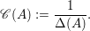 $$\begin{eqnarray}\mathscr{C}(A):=\frac{1}{{\rm\Delta}(A)}.\end{eqnarray}$$
If  $A\in {\rm\Sigma}$, we set
 ${\rm\Delta}(A)=0$ and
 $\mathscr{C}(A)=\infty$.
We have written the definition in such a way that it becomes clear that we measure the relative size of the perturbation for each row  $a_{i}$, where the relativization is with respect to the norm of
 $a_{i}$. Also, it is clear from the definition that
 ${\rm\Delta}(A)$ is scale-invariant in the sense that
 $$\begin{eqnarray}{\rm\Delta}([{\it\lambda}_{1}a_{1},\ldots ,{\it\lambda}_{n}a_{n}])={\rm\Delta}([a_{1},\ldots ,a_{n}])\quad \text{for}~{\it\lambda}_{i}>0.\end{eqnarray}$$
For the analysis of  ${\rm\Delta}$ we may therefore assume, without loss of generality, that
 $\Vert a_{i}\Vert =1$ for all
 $i$. Hence we can see the matrix
 $A$ with columns
 $a_{1},\ldots ,a_{n}$ as an element in the product
 $(\mathbb{S}^{m-1})^{n}$ of spheres. The scale invariance of
 $\mathscr{C}(A)$, together with the characterization
 $$\begin{eqnarray}\Vert A\Vert _{12}=\max _{i\leq n}\Vert a_{i}\Vert\end{eqnarray}$$
immediately yields the following result.
 $$\begin{eqnarray}\mathscr{C}(A)=\frac{\Vert A\Vert _{12}}{d_{12}(A,{\rm\Sigma})}.\square\end{eqnarray}$$
A number of different characterizations of  $\mathscr{C}(A)$ are shown in Bürgisser and Cucker (Reference Bürgisser and Cucker2013, Chapter 6).
(b) Algorithms and complexity.
During the late 1970s and early 1980s two algorithms proved that linear programming problems (with integer coefficients) can be solved in polynomial time: the ellipsoid algorithm and interior-point methods. These algorithms are naturally described as real number algorithms. But when considered over real (as opposed to integer) data their halting time is no longer bounded by a function of the input size only. Instead, the condition of the data at hand appears to play a role.
Of course, one may argue that the condition of the data is now replacing the bit-size of the largest component in this data. But the fact remains that this bit-size is directly related to the size of the input whereas the condition of the input is not (and it is not even known a priori).
Of these two methods, the most efficient (both in theory and in practice) is the interior-point method. There is a vast literature on this method (the book by Renegar Reference Renegar2000 being a very good introduction to them for general conic programming). For our purposes, it should suffice to state a result with the complexity of an interior-point algorithm solving the polyhedral cone feasibility problem. The proof of this result (and a self-contained introduction to interior-point methods for linear programming) can be found in Chapter 9 of Bürgisser and Cucker (Reference Bürgisser and Cucker2013).
Theorem 3.28. We exhibit an interior-point algorithm which, on input  $A\not \in {\rm\Sigma}$, returns either a strictly feasible primal solution, i.e., a point
 $x\in \mathbb{R}^{n}$ such that
 $Ax=0$,
 $x>0$, or a strictly feasible dual solution, i.e., a point
 $y\in \mathbb{R}^{m}$ such that
 $A^{\text{T}}y<0$. In both cases, the algorithm halts after at most
 $$\begin{eqnarray}O(\sqrt{n}(\log n+\log \mathscr{C}(A)))\end{eqnarray}$$
iterations. The total number of arithmetic operations is bounded by
 $$\begin{eqnarray}O(n^{3.5}(\log n+\log \mathscr{C}(A))).\square\end{eqnarray}$$
A version of this result which takes into consideration the effects of finite precision, and shows complexity bounds of the same order, can be found in Cucker and Peña (Reference Cucker and Peña2002).
(c) Condition of random data.
Theorem 3.28 is an instance of a common phenomenon in the analysis of iterative algorithms (which we already met regarding the conjugate gradient method). The cost of each iteration is bounded by a function of the size or dimension of the input (in our case, it is  $O(n^{3})$ where, we recall,
 $A\in \mathbb{R}^{m\times n}$ with
 $n>m$) but the number of iterations performed by the algorithm depends on the condition of the input at hand. To get an idea of how efficient the algorithm is ‘in general’, a probabilistic analysis is a must.
There is a sequence of papers on probabilistic analyses of  $\mathscr{C}(A)$. The sharpest bound for the expectation of
 $\log \mathscr{C}(A)$ appears in Bürgisser, Cucker and Lotz (Reference Bürgisser, Cucker and Lotz2010). It shows that
 $$\begin{eqnarray}\mathbb{E}_{A\sim N(0,\text{Id})}\ln \mathscr{C}(A)\leq 2\ln (m+1)+3.31.\end{eqnarray}$$
As for a smoothed analysis, Amelunxen and Bürgisser (Reference Amelunxen and Bürgisser2012) showed that
 $$\begin{eqnarray}\sup _{\overline{A}\in (\mathbb{S}^{m-1})^{n}}\mathbb{E}_{A\sim N(\overline{A},{\it\sigma}^{2}\text{Id})}\log \mathscr{C}(A)=O\biggl(\log \frac{n}{{\it\sigma}}\biggr).\end{eqnarray}$$
These two bounds carry a very clear message: the cost of solving a typical polyhedral feasibility problem (or a typical perturbation of an arbitrary one) is  $O(n^{3.5}\log n)$. The contribution of the condition of the input to this cost is very minor.
3.6 Linear programming
(a) The problem.
The linear programming problem in standard form is to find  $x\in \mathbb{R}^{n}$ solving

where  $A\in \mathbb{R}^{m\times n}$,
 $b\in \mathbb{R}^{m}$ and
 $c\in \mathbb{R}^{n}$ are given. The well-known Duality Theorem states that if a minimizer
 $x^{\ast }$ exists then a maximizer
 $y^{\ast }$ exists as well for the dual problem

and we have  $c^{\text{T}}x^{\ast }=b^{\text{T}}y^{\ast }$. It additionally ensures that this is the case if and only if both the primal and dual are feasible. That is, there exists a pair
 $(x,y)\in \mathbb{R}^{n+m}$ such that
 $Ax=b$,
 $x\geq 0$ and
 $A^{\text{T}}y\leq c$. In this case, we say that the triple
 $d=(A,b,c)$ is feasible.
For any subset  $B$ of
 $\{1,2,\ldots ,n\}$, we let
 $A_{B}$ denote the submatrix of
 $A$ obtained by removing from
 $A$ all the columns with index not in
 $B$. If
 $x\in \mathbb{R}^{n}$,
 $x_{B}$ is defined analogously. Also, let
 $N:=\{1,2,\ldots ,n\}\setminus B$. Then
 $A_{N}$ and
 $x_{N}$ are defined similarly. We say that
 $B$ is a basis for
 $d=(A,b,c)$ when
 $|B|=m$ and
 $A_{B}$ is invertible.
In this case, we may solve  $A_{B}x=b$. Consider the point
 $x^{\ast }\in \mathbb{R}^{n}$ defined by
 $x_{N}^{\ast }=0$ and
 $x_{B}^{\ast }=x$. Clearly,
 $Ax^{\ast }=b$. We say that
 $x^{\ast }$ is the primal basic solution of (OP) associated with
 $B$. If, in addition,
 $x^{\ast }\geq 0$, which is equivalent to
 $x_{B}^{\ast }\geq 0$, then we say that
 $x^{\ast }$ is a primal basic feasible solution.
Similarly, we may solve  $A_{B}^{\text{T}}y=c_{B}$. The point
 $y^{\ast }$ thus obtained is said to be the dual basic solution of associated with
 $B$. If, in addition,
 $A^{\text{T}}y^{\ast }\leq c$, then
 $y^{\ast }$ is said to be a dual basic feasible solution.
Definition 3.29. A basis  $B$ for a data triple
 $d$ is called an optimal basis if both the primal and dual basic solutions associated with
 $B$ are feasible, in which case the latter are called the basic optimal solutions of
 $d$ associated with
 $B$.
There is a rationale for the word ‘optimal’ in this definition. If  $B$ is an optimal basis and
 $x^{\ast },y^{\ast }$ are its associated basic optimal solutions, then
 $x^{\ast }$ and
 $y^{\ast }$ are optimizers for the problems (OP) and (OD), respectively. Furthermore, optimal bases exist (Bürgisser and Cucker Reference Bürgisser and Cucker2013, Theorem 8.13).
Theorem 3.30. Let  $d=(A,b,c)$ be a data triple satisfying
 $\mathsf{rank}\,A=m$.
(a) There is an optimal basis for
$d$ if and only if both (OP) and (OD) are feasible.(b) Let
$B$ be a basis for $d$. Then $B$ is optimal if and only if both the primal and the dual basic solutions associated with $B$ are optimizers for (OP) and (OD) respectively.(c) If there is more than one optimal basis, say
$B_{1},\ldots ,B_{s}$, $s\geq 2$, then the set of optimizers for (OP) contains the convex hull of $x_{1}^{\ast },\ldots ,x_{s}^{\ast }$, where $x_{i}^{\ast }\in \mathbb{R}^{n}$ is the primal basic solution associated with $B_{i}$, $i=1,\ldots ,s$. Likewise for the set of optimizers for (OD) ◻


Theorem 3.30 suggests a strategy to compute optimizers for feasible data with full-rank matrices, namely, to compute an optimal basis  $B$ and its associated basic solutions
 $x^{\ast }$ and
 $y^{\ast }$. These points are vertices in the polyhedra of feasible points for (OP) and (OD), respectively. The simplex algorithm searches for such a solution by examining a cleverly constructed sequence in this set of vertices. Interior-point methods instead produce a sequence of points in the interior of these polyhedra that leads to the desired vertex.
(b) Ill-posedness and condition.
The problems of computing optimizers and optimal bases are, strictly speaking, different. But both their sets of ill-posed data and their condition numbers are, as one can expect, very closely related.
Even though we will only be interested in feasible data (in this example we compute optimizers for data of this type) we still need to mention infeasible data at the boundary of the set of feasible data. A more detailed discussion of ill-posedness, with connections to the notion of degeneracy, can be found in Bürgisser and Cucker (Reference Bürgisser and Cucker2013, § 8.4).
We observe that infeasible triples should be considered as ill-posed if and only if arbitrarily small perturbations can make these triples feasible (and, consequently, create optimizers for them). We thus define
 $$\begin{eqnarray}{\rm\Sigma}_{{\mathcal{I}}}:=\{d\mid d\text{ is infeasible and }\forall {\it\varepsilon}>0\;\exists d^{\prime }\text{feasible with }\Vert d-d^{\prime }\Vert \leq {\it\varepsilon}\}\end{eqnarray}$$
and call this the set of infeasible ill-posed triples.
For the problem of computing optimizers one can show that the property of having more than one pair  $(x^{\ast },y^{\ast })$ of optimizers can be destroyed by arbitrarily small perturbations of the triple
 $d=(A,b,c)$. Also, for problems having a unique pair of optimizers, small perturbations of the data will preserve this character and the resulting pair of optimizers will be close to the original one. Consequently, we define the set of ill-posed triples for this problem to be
 $$\begin{eqnarray}{\rm\Sigma}_{\mathsf{opt}}:=\{d\mid d\text{ has at least two optimizers }(x,y)\}\cup {\rm\Sigma}_{{\mathcal{I}}}.\end{eqnarray}$$
Let us focus next on the problem of computing an optimal basis. In contrast with the preceding problem, this one is discrete-valued: the output for any given datum  $d$ is an
 $m$-element subset in
 $[n]$. Therefore, we can take the set
 ${\rm\Sigma}_{\mathsf{OB}}$ of ill-posed triples as the boundary between these possible outputs. In other words, if
 $\mathsf{OB}(d)$ denotes the set of optimal bases for a triple
 $d$, we define
 $$\begin{eqnarray}{\rm\Sigma}_{\mathsf{OB}}:=\{d\mid \forall {\it\varepsilon}>0\;\exists d^{\prime }~\text{such that}~\mathsf{OB}(d)\neq \mathsf{OB}(d^{\prime })~\text{and}~\Vert d-d^{\prime }\Vert \leq {\it\varepsilon}\}.\end{eqnarray}$$
Note that  ${\rm\Sigma}_{{\mathcal{I}}}$ corresponds to triples
 $d$ in
 ${\rm\Sigma}_{\mathsf{OB}}$ with
 $\mathsf{OB}(d)=\emptyset$.
Proposition 3.31. Let  $d=(A,b,c)$ be feasible. Then we have
 $d\in {\rm\Sigma}_{\mathsf{opt}}\;\Longleftrightarrow \;d\in {\rm\Sigma}_{\mathsf{OB}}$. Furthermore, if
 $\mathsf{rank}\,A<m$ then
 $d\in {\rm\Sigma}_{\mathsf{OB}}$.◻
Following the above we say that  $d$ is feasible well-posed when there exists a unique optimal solution
 $(x^{\ast },y^{\ast })$ for
 $d$. In this case, we write
 $d\in {\mathcal{W}}$. If more than one optimal solution exists, we say that
 $d$ is feasible ill-posed.
Let  ${\mathcal{B}}:=\{B\subseteq [n]\mid |B|=m\}$. Theorem 3.30(c) implies that if
 $d\in {\mathcal{W}}$ is feasible well-posed with optimal solution
 $(x^{\ast },y^{\ast })$, then there is a unique
 $B\in {\mathcal{B}}$ such that
 $(x^{\ast },y^{\ast })$ is the basic optimal solution associated with
 $B$. We may then define, for any
 $B\in {\mathcal{B}}$, the set
 $$\begin{eqnarray}{\mathcal{W}}_{B}:=\{d\in {\mathcal{W}}\mid B\text{ is the optimal basis for }d\}.\end{eqnarray}$$
The set  ${\mathcal{W}}$ is thus partitioned by the family
 $\{{\mathcal{W}}_{B}\mid B\in {\mathcal{B}}\}$. Figure 3.1 schematically summarizes the situation in the space of data.
The situation in the space of data.
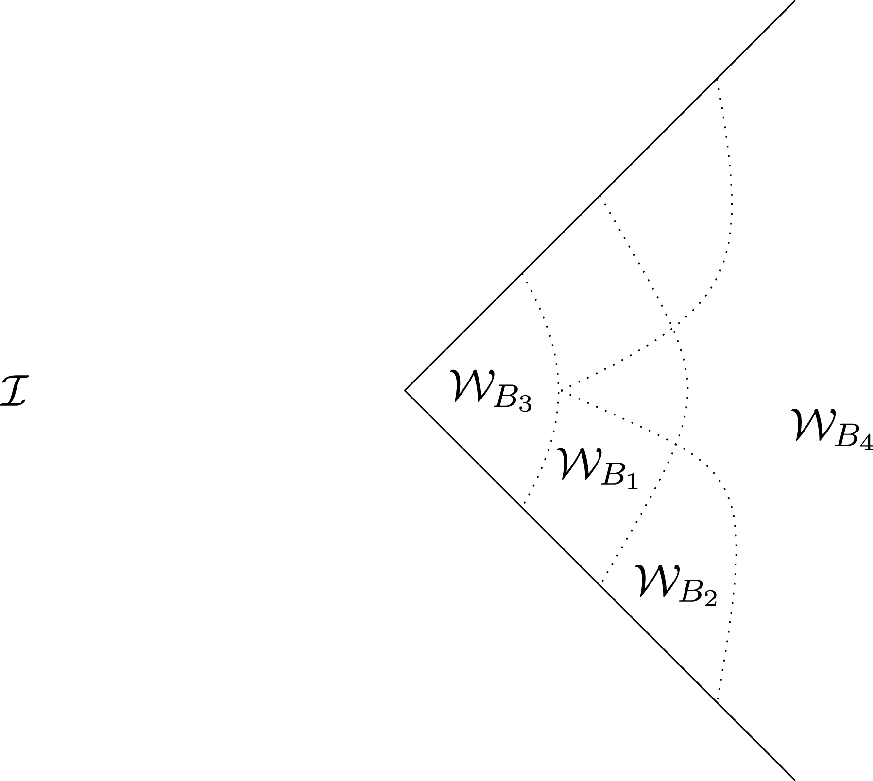
The left of the diagram is not relevant to us: it represents the set  ${\mathcal{I}}$ of infeasible triples. At the right of the diagram we have the set
 ${\mathcal{W}}$ of well-posed feasible triples, which is partitioned into the subsets
 ${\mathcal{W}}_{B}$. The dotted lines separating these subsets correspond to data with more than one optimal basis. The two continuous segments are the boundary between feasible and infeasible triples. The union of these lines – the dotted lines and the continuous segments – forms the set
 ${\rm\Sigma}_{\mathsf{opt}}={\rm\Sigma}_{\mathsf{OB}}$ of ill-posed triples for both the optimal solution and the optimal basis problems.
The picture we just described allows for a very natural definition of condition number. We only need a norm in the space of data triples, and for this we take
 $$\begin{eqnarray}\Vert d\Vert =\biggl\|\left(\begin{array}{@{}cc@{}}A & b\\ c^{\text{T}} & 0\end{array}\right)\biggr\|.\end{eqnarray}$$
Definition 3.32. Let  $d$ be feasible well-posed. We define the distance to ill-posedness to be
 $$\begin{eqnarray}{\it\varrho}(d)=\inf \{\Vert {\rm\Delta}d\Vert \mid d+{\rm\Delta}d\in {\rm\Sigma}_{\mathsf{opt}}\}.\end{eqnarray}$$
Moreover, we define the RCC condition number  $\mathscr{K}(d)$ of
 $d$ by
 $$\begin{eqnarray}\mathscr{K}(d)=\frac{\Vert d\Vert }{{\it\varrho}(d)}.\end{eqnarray}$$
If  $d$ is feasible but not well-posed, we let
 ${\it\varrho}(d)=0$ and
 $\mathscr{K}(d)=\infty$.
(c) Algorithms and complexity.
There is no shortage of algorithms for the linear programming optimization problem. A distinctive feature of the one described in Cheung and Cucker (Reference Cheung and Cucker2006) is that it works with finite precision. Another feature is that both complexity and accuracy are analysed in terms of  $\mathscr{K}(d)$ (which, somewhat conveniently, was introduced and studied in Cheung and Cucker Reference Cheung and Cucker2004).
Theorem 3.33. There exists a finite-precision algorithm which, given a feasible well-posed triple  $d=(A,b,c)$, finds an optimal basis
 $B$ for
 $d$. The machine precision varies during the execution of the algorithm (allowing for rereading the input
 $d$ with higher accuracy) and the finest required precision satisfies
 $$\begin{eqnarray}{\it\epsilon}_{\mathsf{mach}}^{\ast }=\frac{1}{O((m+n+1)^{26}\mathscr{K}(d)^{16})}.\end{eqnarray}$$
The total number of arithmetic operations is bounded by
 $$\begin{eqnarray}O(n^{3.5}(\log n+\log \mathscr{K}(d))\log \log (\mathscr{K}(d)+1)).\square\end{eqnarray}$$
The feasibility of the triple  $d$ needs to be ascertained before the execution of the algorithm in Theorem 3.33, but it is shown in Cheung and Cucker (Reference Cheung and Cucker2006) that this can be done within the accuracy and complexity bounds in the theorem.
The bound for  ${\it\epsilon}_{\mathsf{mach}}^{\ast }$ shows that the largest number of digits needed for the floating-point numbers occurring during the computation is bounded as
 $$\begin{eqnarray}O(\log (n)+\log \mathscr{K}(d)).\end{eqnarray}$$
In Bürgisser and Cucker (Reference Bürgisser and Cucker2013, Chapter 11) there is a version of Theorem 3.33 for infinite precision. Needless to say, the corresponding proof is much simplified. There is also a description of a different algorithm with a slightly smaller complexity bound (without the  $\log \log \mathscr{K}(d)$ factor) but requiring an initial pair
 $(x_{0},y_{0})$ satisfying some properties.
One final remark is essential. Once we have computed the optimal basis  $B$ for the triple
 $d$ we still want to compute the optimizers. For this, recall that we need to compute
 $$\begin{eqnarray}x_{B}^{\ast }=A_{B}^{-1}b\quad \text{and}\quad y^{\ast }=A_{B}^{-\text{T}}c_{B}.\end{eqnarray}$$
Whereas the complexity of this computation is dominated by that of computing  $B$, its accuracy analysis (such as the one in Section 3.1) depends on
 ${\it\kappa}(A_{B})={\it\kappa}(A_{B}^{\text{T}})$. However, the inequality
 $$\begin{eqnarray}{\it\kappa}(A_{B})\leq \mathscr{K}(d)\end{eqnarray}$$
(see Bürgisser and Cucker Reference Bürgisser and Cucker2013, Proposition 11.22) reduces all our needs to one: understanding how large  $\mathscr{K}(d)$ is in general.
(d) Probabilistic analyses.
An average analysis of  $\mathscr{K}(d)$ was obtained in Cheung and Cucker (Reference Cheung and Cucker2013).
Theorem 3.34. We have
 $$\begin{eqnarray}\mathbb{E}_{d\sim N(0,\text{Id})}(\log \mathscr{K}(d)\mid d\in {\mathcal{W}})\leq \frac{5}{2}\log (n+1)+\log (m+1)+\log 24e,\end{eqnarray}$$
as well as
 $$\begin{eqnarray}\mathbb{E}_{d\sim N(0,\text{Id})}(\log \log \mathscr{K}(d)\mid d\in {\mathcal{W}})=\log \log n+O(1)\end{eqnarray}$$
and
 $$\begin{eqnarray}\mathbb{E}_{d\sim N(0,\text{Id})}(\log \mathscr{K}(d)\log \log \mathscr{K}(d)\mid d\in {\mathcal{W}})=\log n\log \log n+O(1).\square\end{eqnarray}$$
Theorems 3.33 and 3.34 combine to yield the following.
Corollary 3.35. There exists a finite-precision algorithm that, given a triple  $d=(A,b,c)$, finds an optimal basis
 $B$ for
 $d$. The average cost of the algorithm, on Gaussian data
 $d$, conditioned to
 $d$ being feasible well-posed, is bounded by
 $$\begin{eqnarray}O(n^{3.5}\log n\log \log n).\end{eqnarray}$$
The machine precision varies during the execution of the algorithm. The largest number of digits needed for the floating-point numbers occurring in the computation is bounded on average as
 $$\begin{eqnarray}\mathbb{E}_{d\sim N(0,\text{Id})}\log {\it\epsilon}_{\mathsf{mach}}^{\ast }(d)=O(\log n).\square\end{eqnarray}$$
Remarkably, as of today, the problem of showing a smoothed analysis version of Theorem 3.34 remains open.
3.7 Homotopy methods
In all the previous examples, the behaviour of an algorithm (either with respect to numerical stability or with respect to complexity) is determined by, in addition to size, the condition of the input at hand. The examples in the next two paragraphs showcase a more intricate situation in which the complexity of an execution depends on the condition of an infinite collection of objects, namely a curve in the product space  $X\times Y$, where
 $X$ is a manifold of inputs and
 $Y$ a manifold of solutions. We are therefore in the framework described in Section 1.1(b), which the reader might want to refresh before continuing.
In our context, it will be convenient to look at the elements in the manifold of inputs as functions defined on  $Y$ with values on some linear space. The computational problem is, given
 $f\in X$, find
 $y\in Y$ such that
 $f(y)=0$. Homotopy (or continuation) methods are a family of algorithms that do just this. They require a pair
 $(g,{\it\zeta})$ at hand with
 $g\in X$ and
 ${\it\zeta}\in Y$ a zero of
 $g$.
The general idea of the method is to consider a path
 $$\begin{eqnarray}{\it\gamma}:[0,1]\rightarrow X,\quad t\mapsto q_{t},\end{eqnarray}$$
such that  $q_{0}=g$ and
 $q_{1}=f$. This path needs to be computable (in the sense that
 $q_{t}$ may be computed from
 $f,g$, and
 $t$).
Under certain conditions the path  ${\it\gamma}$ can be lifted to a path
 ${\it\Gamma}$ in the solution manifold
 $V\subset X\times Y$ such that
 ${\it\Gamma}(0)=(q_{0},{\it\zeta})$. If this is the case, by projecting onto
 $Y$ we obtain a path
 $\{{\it\zeta}_{t}\}_{t\in [0,1]}$ on
 $Y$ such that
 ${\it\zeta}_{0}={\it\zeta}$ and
 $f({\it\zeta}_{1})=0$. The goal of homotopy methods is to ‘follow’ (or ‘continue’) the path on
 $V$ to eventually obtain an approximation of
 ${\it\zeta}_{1}$. The algorithmic scheme, broadly described, is shown in Algorithm 2. Figure 3.2 attempts to give an idea of this process.
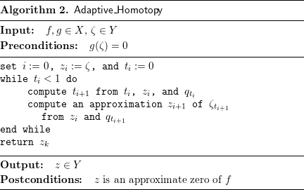
The continuation of the solution path.
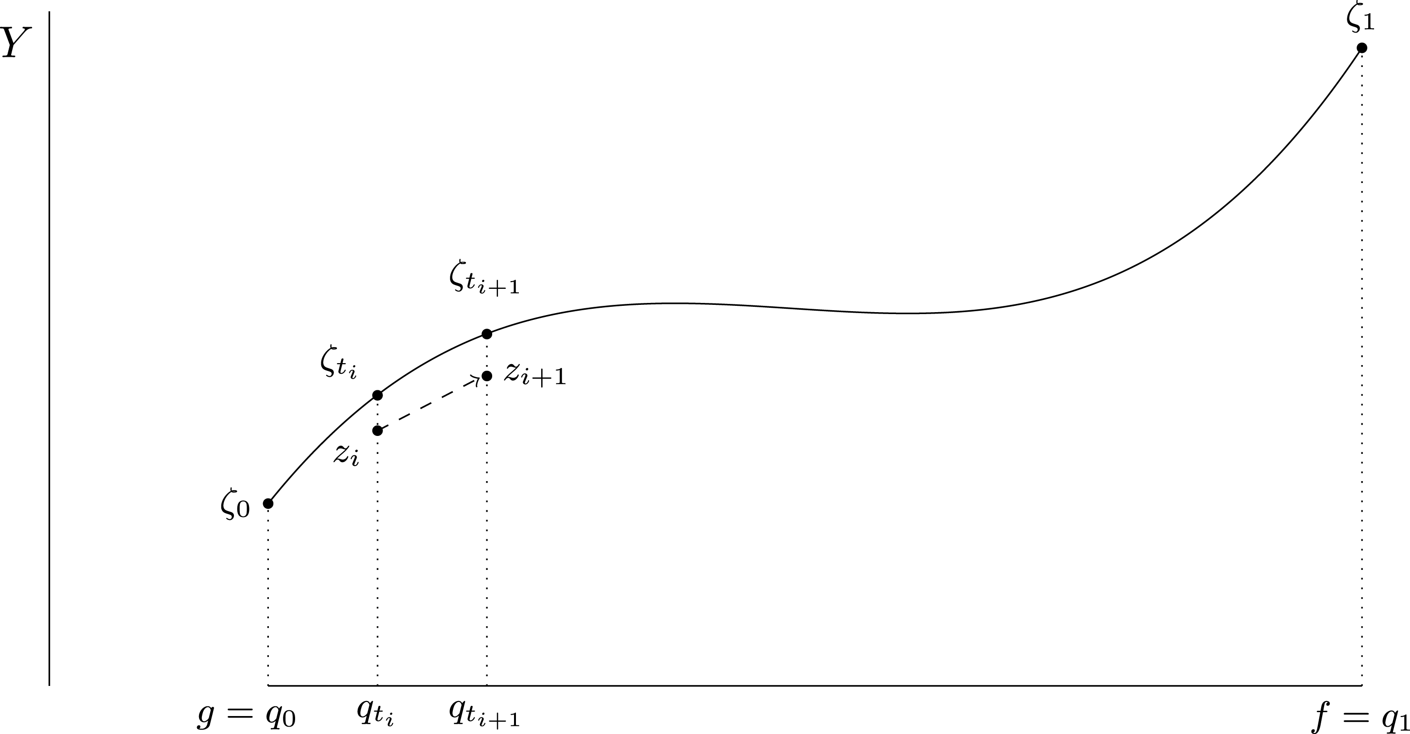
To turn this broad description into a working algorithm, a number of issues need to be clarified: What is ‘an approximation’  $z$ of a zero
 ${\it\zeta}_{t}$ of
 $q_{t}$? How are the approximations
 $z_{i}$ computed? How are the points
 $t_{i}$ computed?
It turns out that Newton’s method and Smale’s theory of approximate zeros give an elegant answer to these questions.
When we talk about Newton’s method we are referring to a general idea that is adapted to different contexts. The general idea is that to a function  $f:Y\rightarrow \mathbb{C}^{n}$ we associate its Newton’s operator
 $N_{f}:Y\rightarrow Y$, which is defined almost everywhere on
 $Y$. The key property of this operator is that if we start from a point
 $z_{0}\in Y$ sufficiently close to a simple zero
 ${\it\zeta}$ of
 $f$ and we iteratively compute its image under
 $N_{f}$, then the resulting sequence converges immediately and quadratically fast to
 ${\it\zeta}$. Newton’s method does not actually find a zero of
 $f$, but starting with a modest approximation of such a zero, it refines its accuracy in a very fast manner.
To make this notion into a definition we assume a distance  $\mathsf{dist}$ on
 $Y$.
Definition 3.36. We say that  $z\in Y$ is an approximate zero of
 $f$ if the sequence given by
 $z_{0}=z$ and
 $z_{i+1}=N_{f}(z_{i})$ is defined for all natural numbers
 $i$, and there is a
 ${\it\zeta}$ with
 $f({\it\zeta})=0$ such that, for all
 $i\in \mathbb{N}$,
 $$\begin{eqnarray}\mathsf{dist}(z_{i}-{\it\zeta})\leq \biggl(\frac{1}{2}\biggr)^{2^{i}-1}\,\mathsf{dist}(z-{\it\zeta}).\end{eqnarray}$$
We say that  ${\it\zeta}$ is the associated zero of
 $z$.
This definition gives an answer to one of our questions above, What is an approximation of a zero? Newton’s method itself gives an answer to another of these questions, How are the  $z_{i}$ computed? Indeed, we make the second computation in the while loop in Algorithm 2 precise by taking
 $$\begin{eqnarray}\mathtt{compute}~z_{i+1}:=N_{q_{t_{i+1}}}(z_{i}).\end{eqnarray}$$
It remains to give an answer to the third question: How are the points  $t_{i}$ computed? That is, how do we compute
 $t_{i+1}$ from
 $t_{i}$,
 $z_{i}$, and
 $q_{t_{i}}$?
The short answer is: we choose  $t_{i+1}$ so that
 $z_{i}$ is an approximate zero of
 $q_{t_{i+1}}$.
Procedures for a choice of  $t_{i+1}$ ensuring this property turn out to be easy to implement and difficult to justify. In all cases, they rely on an estimate of the size of the basin of quadratic attraction of
 $f\in X$ around a zero
 ${\it\zeta}$. That is, how large is the set
 $$\begin{eqnarray}\{z\in Y\mid z\text{ is an approximate zero of }f\text{ with associated zero }{\it\zeta}\}.\end{eqnarray}$$
Smale’s Gamma theory gives an answer to this question in terms of a quantity  ${\it\gamma}(f,{\it\zeta})$ that relates to Hadamard’s formula for the radius of convergence of an analytic function around a given point. As it happens,
 ${\it\gamma}(f,{\it\zeta})$ is closely related to condition as well.
The combination of  $z_{i}$ being an approximate zero of
 $q_{t_{i+1}}$ and
 $z_{i+1}$ being defined as
 $N_{q_{t_{i+1}}}(z_{i})$ ensures that, for all
 $i$, the point
 $z_{i}$ is very close to the zero
 ${\it\zeta}_{i}$. Figure 3.3 depicts the situation. The curve in the centre is the lifted path
 ${\it\Gamma}\subset V$, that is, the set
 $\{(q_{t},{\it\zeta}_{t})\}_{t\in [0,1]}$. The lightly shaded area is the set of points
 $(q_{t},z)$ such that
 $z$ is an approximate zero of
 $q_{t}$ with associated zero
 ${\it\zeta}_{t}$. The dark shaded area is a contraction of the lightly shaded one centred at
 ${\it\Gamma}$ with coefficient
 $1/2$. The sequence of approximations
 $z_{i}$ lie on this dark shaded region. In a way, they are ‘strong approximate’ zeros.
Approximate and ‘strong approximate’ zeros.
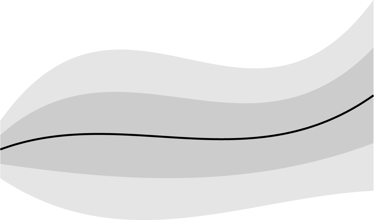
Both the role played by condition numbers in the choice of the homotopy’s step-size and the way they affect the speed of the algorithm will be main characters in the next two examples.
3.8 Smale’s 17th problem
(a) The problem.
Let  $\mathbf{d}=(d_{1},\ldots ,d_{n})$ with
 $d_{i}\in \mathbb{N}$,
 $d_{i}\geq 2$. We let
 ${\mathcal{H}}_{\mathbf{d}}$ denote the linear space of homogeneous polynomial systems
 $f=(f_{1},\ldots ,f_{n})$, where
 $f_{i}\in \mathbb{C}[X_{0},\ldots ,X_{n}]$ is homogeneous of degree
 $d_{i}$.
Steve Smale (Reference Smale, Arnold, Atiyah, Lax and Mazur2000) proposed a list of 18 problems for the mathematicians of the twenty-first century. The 17th problem asks whether there exists an algorithm that, given  $f\in {\mathcal{H}}_{\mathbf{d}}$, returns an approximate zero of
 $f$ in time polynomial (on average) in the size of
 $f$. Here ‘approximate zero’ is in the sense of Definition 3.36 (with respect to a projective Newton’s method tailored to this problem by Mike Shub Reference Shub, Hirsch, Marsden and Shub1993) and ‘average’ is with respect to the standard normal distribution for the coefficients of the
 $f_{i}$ when these polynomials are written in the Weyl basis (a simple modification to the usual basis that makes the associated Hermitian product unitarily invariant: for details see Bürgisser and Cucker Reference Bürgisser and Cucker2013, Section 16.1). The ‘size’ of
 $f$ is the total number of these coefficients or, equivalently, the dimension
 $N$ of
 ${\mathcal{H}}_{\mathbf{d}}$ over
 $\mathbb{C}$. This yields
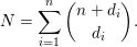 $$\begin{eqnarray}N=\mathop{\sum }_{i=1}^{n}\binom{n+d_{i}}{d_{i}}.\end{eqnarray}$$
Attempts to give an affirmative answer to Smale’s 17th problem have revolved around homotopy algorithms. The works by Beltrán and Pardo (Reference Beltrán and Pardo2009, Reference Beltrán and Pardo2011) provided a partial answer in the form of a randomized algorithm whose expected running time (with respect to both the randomizations and the input  $f$) is polynomial in
 $N$. A further development was given in Bürgisser and Cucker (Reference Bürgisser and Cucker2011), where a deterministic algorithm working in nearly polynomial time was described. All these works heavily relied on the analysis of a condition number. In what follows we define this condition number, specify the choice of step-length in the homotopy algorithm, and show (sketching the proofs) how a smoothed analysis leads to the results mentioned above.
(b) Condition numbers.
To define the condition for Smale’s 17th problem we use the setting described in Section 1.1(b). Here the manifold of inputs is  ${\mathcal{H}}_{\mathbf{d}}$, the manifold of outputs is
 $\mathbb{P}^{n}:=\mathbb{P}(\mathbb{C}^{n+1})$, and the submanifold
 $V\subset {\mathcal{H}}_{\mathbf{d}}\times \mathbb{P}(\mathbb{C}^{n+1})$ of solutions is the set of pairs
 $(f,{\it\zeta})$ with
 $f({\it\zeta})=0$.
It turns out that the set of ill-posed solutions is then (recall (1.6))
 $$\begin{eqnarray}{\rm\Sigma}^{\prime }=\big\{(f,{\it\zeta})\in V\mid \mathsf{rank}\,Df({\it\zeta})<n\big\}\end{eqnarray}$$
and that, for  $(f,{\it\zeta})\in V$,
 $(f,{\it\zeta})\in {\rm\Sigma}^{\prime }$ if and only if
 $z$ is a multiple zero of
 $f$.
Recall the projections  ${\it\pi}_{1}$ and
 ${\it\pi}_{2}$:
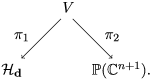
We also define the set  ${\rm\Sigma}:={\it\pi}_{1}({\rm\Sigma}^{\prime })$ consisting of those systems
 $f\in {\mathcal{H}}_{\mathbf{d}}$ that have some multiple zero
 ${\it\zeta}$.
For a pair  $(f_{0},{\it\zeta}_{0})\in V\setminus {\rm\Sigma}^{\prime }$ we have defined the absolute condition number
 $\mathsf{acond}(f_{0},{\it\zeta}_{0})$ to be the operator norm of the solution map
 $G:U\rightarrow \mathbb{P}^{n},G(f)={\it\zeta}$ that locally inverts
 ${\it\pi}_{1}:V\rightarrow {\mathcal{H}}_{\mathbf{d}}$ around
 $(f_{0},{\it\zeta}_{0})$ on an open neighbourhood
 $U$ of
 $f_{0}$ in
 ${\mathcal{H}}_{\mathbf{d}}$. To make the condition independent of the scaling of
 $f$ we take, for
 $(f,{\it\zeta})\in V\setminus {\rm\Sigma}^{\prime }$,
 $$\begin{eqnarray}{\it\mu}(f,{\it\zeta}):=\Vert f\Vert \cdot \Vert DG(f)\Vert ,\end{eqnarray}$$
where the operator norm is with respect to the standard Hermitian product (with respect to the Weyl’s basis) on  ${\mathcal{H}}_{\mathbf{d}}$ and the Hermitian product on
 $T_{{\it\zeta}}\mathbb{P}^{n}$ coming from the standard one on
 $\mathbb{C}^{n+1}$.
The condition number  ${\it\mu}(f,{\it\zeta})$ can also be expressed in terms of the derivative
 $Df({\it\zeta}):\mathbb{C}^{n+1}\rightarrow \mathbb{C}^{n}$ of
 $f:\mathbb{C}^{n+1}\rightarrow \mathbb{C}^{n}$. Euler’s identity implies that
 ${\it\zeta}$ lies in the kernel of
 $Df({\it\zeta})$. So, if
 $Df({\it\zeta})$ is of full rank, its kernel is
 $\mathbb{C}{\it\zeta}$ and
 $T_{{\it\zeta}}$ equals its orthogonal complement. The inverse of the restriction
 $Df({\it\zeta})_{|T_{{\it\zeta}}}$ is described by the Moore–Penrose inverse
 $Df({\it\zeta})^{\dagger }$, and we have
 $$\begin{eqnarray}{\it\mu}(f,{\it\zeta})=\Vert f\Vert \cdot \Vert Df({\it\zeta})^{\dagger }\mathsf{diag}(\Vert {\it\zeta}\Vert ^{d_{i}-1})\Vert .\end{eqnarray}$$
The function  ${\it\mu}$ is a condition number in the classical sense: it bounds the speed of change of the solutions when the data change. Indeed, if
 $[0,1]\rightarrow V,\,t\mapsto (f_{t},{\it\zeta}_{t})\in V$ is a smooth curve such that
 $f_{t}\in \mathbb{S}({\mathcal{H}}_{\mathbf{d}})$ for all
 $t$, then
 $$\begin{eqnarray}\Vert \dot{{\it\zeta}}_{t}\Vert \leq {\it\mu}(f_{t},{\it\zeta}_{t})\Vert \dot{f_{t}}\Vert .\end{eqnarray}$$
For technical reasons, it has proved to be convenient to work with a slight modification to  ${\it\mu}$. We define the normalized condition number
 ${\it\mu}_{\text{norm}}(f,{\it\zeta})$ for
 $(f,{\it\zeta})\in V$ by
 $$\begin{eqnarray}{\it\mu}_{\text{norm}}(f,{\it\zeta}):=\Vert f\Vert \cdot \Vert Df({\it\zeta})^{\dagger }\mathsf{diag}(\sqrt{d_{i}}\Vert {\it\zeta}\Vert ^{d_{i}-1})\Vert .\end{eqnarray}$$
Note that the introduction of the  $\sqrt{d_{i}}$ factors is the only change compared with
 ${\it\mu}(f,{\it\zeta})$. In particular, we have
 $$\begin{eqnarray}{\it\mu}(f,{\it\zeta})\leq {\it\mu}_{\text{norm}}(f,{\it\zeta})\leq \sqrt{D}\,{\it\mu}(f,{\it\zeta})\end{eqnarray}$$
where  $D:=\max _{i}d_{i}$. Furthermore, since our algorithms work with approximations of zeros only, it will be convenient to extend
 ${\it\mu}_{\text{norm}}(f,z)$ to the case that
 $z$ is not a zero of
 $f$.
Definition 3.37. For  $f\in {\mathcal{H}}_{\mathbf{d}}$ and
 $z\in (\mathbb{C}^{n+1})_{\ast }$ we define the normalized condition number
 ${\it\mu}_{\text{norm}}(f,z)$ as
 $$\begin{eqnarray}{\it\mu}_{\text{norm}}(f,z):=\Vert f\Vert \cdot \Vert Df(z)|_{T_{z}}^{-1}\mathsf{diag}(\sqrt{d_{i}}\,\Vert z\Vert ^{d_{i}-1})\Vert\end{eqnarray}$$
if  $Df(z)|_{T_{z}}:T_{z}\rightarrow \mathbb{C}^{n}$ is invertible. Otherwise, we set
 ${\it\mu}_{\text{norm}}(f,z):=\infty$.
By Euler’s identity, if  $f(z)=0$, this is consistent with the original definition (3.18):
 $$\begin{eqnarray}{\it\mu}_{\text{norm}}(f,z)=\Vert f\Vert \cdot \Vert Df(z)^{\dagger }\mathsf{diag}(\sqrt{d_{i}}\Vert z\Vert ^{d_{i}-1})\Vert .\end{eqnarray}$$
We note, however, that using this formula in the case  $f(z)\neq 0$ would lead to a different notion of
 ${\it\mu}_{\text{norm}}(f,z)$ (although the difference is small if
 $z$ is close to
 ${\it\zeta}$).
The condition number  ${\it\mu}_{\text{norm}}$ has several properties. It is invariant under scaling: that is, for
 ${\it\lambda}_{1},{\it\lambda}_{2}\in \mathbb{C}_{\ast }$, we have
 ${\it\mu}_{\text{norm}}({\it\lambda}_{1}f,{\it\lambda}_{2}z)={\it\mu}_{\text{norm}}(f,z)$. It is bounded below:
 ${\it\mu}_{\text{norm}}(f,z)\geq \sqrt{n}$ for all
 $(f,z)\in {\mathcal{H}}_{\mathbf{d}}\times (\mathbb{C}^{n+1})_{\ast }$. And, crucially, it controls the size of the basin of quadratic attraction of
 $f$ around a zero
 ${\it\zeta}$ (see Bürgisser and Cucker Reference Bürgisser and Cucker2011, Theorem 2.2). Let
 $d_{\mathbb{P}}$ denote the Riemannian distance in projective space
 $\mathbb{P}^{n}$ (i.e. the angle).
Theorem 3.38. Let  $(f,{\it\zeta})\in V$ and
 $x\in \mathbb{P}^{n}$ such that
 $$\begin{eqnarray}d_{\mathbb{P}}(x,{\it\zeta})\leq \frac{3-\sqrt{7}}{D^{3/2}{\it\mu}_{\text{norm}}(f,{\it\zeta})}.\end{eqnarray}$$
Then  $x$ is an approximate zero of
 $f$ with associated zero
 ${\it\zeta}$.◻
(c) The homotopy algorithm.
It is this last theorem (along with a bound on the Lipschitz constant for  ${\it\mu}_{\text{norm}}$) that allows for a very simple choice of step-size in the homotopy, namely,
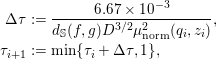 $$\begin{eqnarray}\displaystyle {\rm\Delta}{\it\tau} & := & \displaystyle \frac{6.67\times 10^{-3}}{d_{\mathbb{S}}(f,g)D^{3/2}{\it\mu}_{\text{norm}}^{2}(q_{i},z_{i})},\nonumber\\ \displaystyle {\it\tau}_{i+1} & := & \displaystyle \min \{{\it\tau}_{i}+{\rm\Delta}{\it\tau},1\},\nonumber\end{eqnarray}$$
where  $d_{\mathbb{S}}(f,g)$ denotes the angle between
 $f$ and
 $g$. Algorithm 2 – given a system
 $f$ and an initial pair
 $(g,{\it\zeta})$ – endowed with this choice of step-size returns an approximate zero of
 $f$. The following result (see Bürgisser and Cucker Reference Bürgisser and Cucker2011, Theorem 3.1, or Bürgisser and Cucker Reference Bürgisser and Cucker2013, Theorem 17.3) shows that this is so, and gives a first estimate of the cost of the homotopy.
Theorem 3.39. Suppose that the segment  $[f,g]$ does not intersect the discriminant variety
 ${\rm\Sigma}$. Then the homotopy stops after at most
 $K$ iterations with
 $$\begin{eqnarray}K:=K(f,g,{\it\zeta}):=\leq C\,D^{3/2}\,d_{\mathbb{ S}}(f,g)\int _{0}^{1}{\it\mu}_{\text{norm}}^{2}(q_{{\it\tau}},{\it\zeta}_{{\it\tau}})\,\text{d}{\it\tau}\end{eqnarray}$$
for some constant  $C$. The returned point
 $z$ is an approximate zero of
 $f$ with associated zero
 ${\it\zeta}_{1}$.◻
The number  $K$ of iterations performed by the algorithm is closely related to the total cost since it is easy to see (Bürgisser and Cucker Reference Bürgisser and Cucker2013, Proposition 16.32) that each iteration is performed with
 $O(N)$ arithmetic operations.
We note that the ingredients in the integral in Theorem 3.39, the angular distances and the condition number  ${\it\mu}_{\text{norm}}$ are scale-invariant. This is natural since the number of iterations of the homotopy algorithm is invariant under scaling of
 $f$ and/or
 $g$.
(d) Random data and/or initial pairs.
The bound in Theorem 3.39 depends on an integral which, in turn, depends on  $f$ and the pair
 $(g,{\it\zeta})$. In order to obtain more concrete bounds one needs to eliminate this integral, a computation that requires either specific choices for
 $f$ or
 $(g,{\it\zeta})$ or assumes them drawn from a probability distribution. In the case of
 $f$, the latter amounts to working in the average complexity framework of Smale’s 17th problem. In the case of
 $(g,{\it\zeta})$, it allows for the use of randomized algorithms. For now, we will consider randomizing both
 $f$ and the pair
 $(g,{\it\zeta})$.
Note that to do the latter we need two additional ingredients: a probability measure on the solution manifold  $V$ and an algorithmic procedure to draw pairs from this measure.
For the first, we adopt the measure  ${\it\rho}_{\mathsf{st}}$ (we call it the standard distribution on
 $V$) that is informally described by the following procedure:
 $$\begin{eqnarray}\displaystyle & & \displaystyle \mathtt{draw}~g~\mathtt{from}~N(0,\text{Id})\nonumber\\ \displaystyle & & \displaystyle \mathtt{draw}~{\it\zeta}~\mathtt{from~the~uniform~distribution~on~the}~{\mathcal{D}}~\mathtt{zeros~of}~g\nonumber\end{eqnarray}$$
Here  ${\mathcal{D}}:=\prod _{i=1}^{n}d_{i}$ is the Bézout number. Systems in
 ${\mathcal{H}}_{\mathbf{d}}$ have, with probability 1,
 ${\mathcal{D}}$ different zeros. While this description has the advantage of clarity, it does not suggest an algorithmic procedure to actually draw pairs from
 ${\it\rho}_{\mathsf{st}}$: for this we should have to have at hand the
 ${\mathcal{D}}$ zeros of
 $g$!
Such a procedure (along with the randomization approach for Smale’s 17th problem) was devised by Beltrán and Pardo. It is described in Beltrán and Pardo (Reference Beltrán and Pardo2011) (a more efficient variant can be found in Bürgisser and Cucker Reference Bürgisser and Cucker2013, Section 17.6). It allows for a Las Vegas type algorithm – denoted by  $\mathsf{LV}$ – that, with input
 $f\in {\mathcal{H}}_{\mathbf{d}}$, first draws
 $(g,{\it\zeta})$ from
 $V$ and then computes an approximate zero of
 $f$ by passing
 $f$ and the initial pair
 $(g,{\it\zeta})$ to Algorithm 2.
The central question is: What is the expected complexity of  $\mathsf{LV}$? Here the expectation is with respect to both the input
 $f$ and the pair
 $(g,{\it\zeta})$. The expected number of iterations of the call to Algorithm 2 is then
 $$\begin{eqnarray}\mathbb{E}_{f\sim N(0,\text{Id})}\;\mathbb{E}_{(g,{\it\zeta})\sim {\it\rho}_{\mathsf{st}}}K(f,g,{\it\zeta}),\end{eqnarray}$$
a quantity that, using Theorem 3.39 and the description of  ${\it\rho}_{\mathsf{st}}$, can be bounded by
 $$\begin{eqnarray}CD^{3/2}d_{\mathbb{ S}}(f,g)\mathbb{E}_{f\sim N(0,\text{Id})}\;\mathbb{E}_{g\sim N(0,\text{Id})}\frac{1}{{\mathcal{D}}}\mathop{\sum }_{j=1}^{{\mathcal{D}}}\int _{0}^{1}{\it\mu}_{\text{norm}}^{2}(q_{{\it\tau}},{\it\zeta}_{{\it\tau}}^{(j)})\,\text{d}{\it\tau}.\end{eqnarray}$$
Here 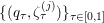 $\{(q_{{\it\tau}},{\it\zeta}_{{\it\tau}}^{(j)})\}_{{\it\tau}\in [0,1]}$ is the lifting of the segment
 $[g,f]$ corresponding to the
 $j$th zero of
 $g$. To further analyse (3.20), we note that neither
 $f$ nor
 $g$ explicitly appears in
 $q_{{\it\tau}}$. They both appear appear implicitly through a complicated function of
 ${\it\tau}$. This function can be simplified by changing the parametrization of the segment
 $[g,f]$ from the ratio
 ${\it\tau}$ of angles to a ratio
 $t$ of Euclidean distances. Elementary geometry shows that this change of parametrization is given by
 $$\begin{eqnarray}t({\it\tau})=\frac{\Vert g\Vert }{\Vert f\Vert (\sin {\it\alpha}\cot ({\it\tau}{\it\alpha})-\cos {\it\alpha})+\Vert g\Vert },\end{eqnarray}$$
where  ${\it\alpha}=d_{\mathbb{S}}(f,g)$; elementary calculus shows that (3.20) is bounded by
 $$\begin{eqnarray}CD^{3/2}d_{\mathbb{ S}}(f,g)\mathbb{E}_{f\sim N(0,\text{Id})}\;\mathbb{E}_{g\sim N(0,\text{Id})}\Vert f\Vert \Vert g\Vert \frac{1}{{\mathcal{D}}}\mathop{\sum }_{j=1}^{{\mathcal{D}}}\int _{0}^{1}\frac{{\it\mu}_{\text{norm}}^{2}(q_{t},{\it\zeta}_{t}^{(j)})}{\Vert q_{t}\Vert ^{2}}\,\text{d}t.\end{eqnarray}$$
A further argument (involving Gaussian distributions truncated at  $\sqrt{2N}$ and scale invariance: see Bürgisser and Cucker Reference Bürgisser and Cucker2011 for details) shows that this last expression is bounded by
 $$\begin{eqnarray}2CD^{3/2}d_{\mathbb{ S}}(f,g)N\mathbb{E}_{f\sim N(0,\text{Id})}\;\mathbb{E}_{g\sim N(0,\text{Id})}\frac{1}{{\mathcal{D}}}\mathop{\sum }_{j=1}^{{\mathcal{D}}}\int _{0}^{1}\frac{{\it\mu}_{\text{norm}}^{2}(q_{t},{\it\zeta}_{t}^{(j)})}{\Vert q_{t}\Vert ^{2}}\,\text{d}t.\end{eqnarray}$$
Further, Tonelli’s theorem allows us to move the integral to the left of the expectations and obtain
 $$\begin{eqnarray}2CD^{3/2}d_{\mathbb{ S}}(f,g)N\int _{0}^{1}\mathbb{E}_{f\sim N(0,\text{Id})}\;\mathbb{E}_{g\sim N(0,\text{Id})}\frac{{\it\mu}_{\mathsf{av}}^{2}(q_{t})}{\Vert q_{t}\Vert ^{2}}\,\text{d}t,\end{eqnarray}$$
where
 $$\begin{eqnarray}{\it\mu}_{\mathsf{av}}^{2}(q_{t}):=\frac{1}{{\mathcal{D}}}\mathop{\sum }_{j=1}^{{\mathcal{D}}}{\it\mu}_{\text{norm}}^{2}(q_{t},{\it\zeta}_{t}^{(j)})\end{eqnarray}$$
is the mean square condition number of  $q_{t}$. The advantage of (3.21) is that, for a fixed
 $t\in [0,1]$, the distribution of
 $q_{t}=tf+(1-t)g$ is Gaussian with centre
 $0$ and covariance matrix
 $(t^{2}+(1-t)^{2})\text{Id}$. That is, we can replace (3.21) with the simpler expression
 $$\begin{eqnarray}2CD^{3/2}d_{\mathbb{ S}}(f,g)N\int _{0}^{1}\mathbb{E}_{q_{t}\sim N(0,(t^{2}+(1-t)^{2})\text{Id})}\;\frac{{\it\mu}_{\mathsf{av}}^{2}(q_{t})}{\Vert q_{t}\Vert ^{2}}\,\text{d}t.\end{eqnarray}$$
We are therefore left with a need to bound the expectation in this expression (for a fixed  $t\in [0,1]$). Before proceeding with this task, though, it will be useful to discuss the more involved framework of a deterministic choice of the initial system
 $g$.
For the time being, we will still assume such a  $g$ in the sphere
 $\mathbb{S}({\mathcal{H}}_{\mathbf{d}})$ and a zero
 ${\it\zeta}$ of
 $g$ which is randomly chosen (as is the input
 $f$). In this case, the reasoning above, replacing the starting bound (3.20) with
 $$\begin{eqnarray}CD^{3/2}d_{\mathbb{ S}}(f,g)\mathbb{E}_{f\sim N(0,\text{Id})}\;\frac{1}{{\mathcal{D}}}\mathop{\sum }_{j=1}^{{\mathcal{D}}}\int _{0}^{1}{\it\mu}_{\text{norm}}^{2}(q_{{\it\tau}},{\it\zeta}_{{\it\tau}}^{(j)})\,\text{d}{\it\tau},\end{eqnarray}$$
ends with the bound
 $$\begin{eqnarray}CD^{3/2}d_{\mathbb{ S}}(f,g)\sqrt{2N}\Vert g\Vert \int _{0}^{1}\mathbb{E}_{q_{t}\sim N((1-t)g,t^{2}\text{Id})}\;\frac{{\it\mu}_{\mathsf{av}}^{2}(q_{t})}{\Vert q_{t}\Vert ^{2}}\,\text{d}t.\end{eqnarray}$$
Again, we are left with a need to bound the expectation in this expression, but this time the expectation leads to a smoothed (as opposed to average) analysis.
(e) Smoothed analysis of${\it\mu}_{\mathsf{av}}^{2}(q)/\Vert q\Vert ^{2}$.

This is the most technically involved part of the example. The result (see Bürgisser and Cucker Reference Bürgisser and Cucker2011 § 8, for details of the proof) is as follows.
Theorem 3.40. For  $\overline{q}\in {\mathcal{H}}_{\mathbf{d}}$ and
 ${\it\sigma}>0$ we have
 $$\begin{eqnarray}\mathbb{E}_{q\sim N(\overline{q},{\it\sigma}^{2}\text{Id})}\biggl(\frac{{\it\mu}_{\mathsf{av}}^{2}(q)}{\Vert q\Vert ^{2}}\biggr)\leq \frac{e(n+1)}{2{\it\sigma}^{2}}.\end{eqnarray}$$
Sketch of the proof.
For  ${\it\zeta}\in (\mathbb{C}^{n+1})_{\ast }$ we consider the subspace
 $R_{{\it\zeta}}$ of
 ${\mathcal{H}}_{\mathbf{d}}$ consisting of all systems
 $h$ that vanish at
 ${\it\zeta}$ to higher order:
 $$\begin{eqnarray}R_{{\it\zeta}}:=\big\{h\in {\mathcal{H}}_{\mathbf{d}}\mid h({\it\zeta})=0,Dh({\it\zeta})=0\big\}.\end{eqnarray}$$
We further decompose the orthogonal complement  $R_{{\it\zeta}}^{\bot }$ of
 $R_{{\it\zeta}}$ in
 ${\mathcal{H}}_{\mathbf{d}}$. Let
 $L_{{\it\zeta}}$ denote the subspace of
 $R_{{\it\zeta}}^{\bot }$ consisting of the systems vanishing at
 ${\it\zeta}$, and let
 $C_{{\it\zeta}}$ denote its orthogonal complement in
 $R_{{\it\zeta}}^{\bot }$. Then we have an orthogonal decomposition
 $$\begin{eqnarray}{\mathcal{H}}_{\mathbf{d}}=C_{{\it\zeta}}\oplus L_{{\it\zeta}}\oplus R_{{\it\zeta}}\end{eqnarray}$$
parametrized by  ${\it\zeta}\in (\mathbb{C}^{n+1})_{\ast }$. Note that the spaces
 $C_{{\it\zeta}}$,
 $L_{{\it\zeta}}$, and
 $R_{{\it\zeta}}$ depend only on
 $[{\it\zeta}]\in \mathbb{P}^{n}$.
Let  ${\it\varphi}_{{\mathcal{H}}_{\mathbf{d}}}$ denote the density of the Gaussian
 $N(\overline{q},{\it\sigma}^{2}\text{Id})$ on
 ${\mathcal{H}}_{\mathbf{d}}$, where
 $\overline{q}\in {\mathcal{H}}_{\mathbf{d}}$ and
 ${\it\sigma}>0$. For fixed
 ${\it\zeta}\in \mathbb{S}(\mathbb{C}^{n+1})$ we decompose the mean
 $\overline{q}$ as
 $$\begin{eqnarray}\overline{q}=\overline{k}_{{\it\zeta}}+\overline{g}_{{\it\zeta}}+\overline{h}_{{\it\zeta}}\in C_{{\it\zeta}}\oplus L_{{\it\zeta}}\oplus R_{{\it\zeta}}\end{eqnarray}$$
according to (3.24). If we denote by  ${\it\varphi}_{C_{{\it\zeta}}}$,
 ${\it\varphi}_{L_{{\it\zeta}}}$, and
 ${\it\varphi}_{R_{{\it\zeta}}}$ the densities of the Gaussian distributions in the spaces
 $C_{{\it\zeta}}$,
 $L_{{\it\zeta}}$, and
 $R_{{\it\zeta}}$ with covariance matrices
 ${\it\sigma}^{2}\text{Id}$ and means
 $\overline{k}_{{\it\zeta}},\overline{M}_{{\it\zeta}}$, and
 $\overline{h}_{{\it\zeta}}$, respectively, then the density
 ${\it\varphi}_{{\mathcal{H}}_{\mathbf{d}}}$ factors as
 $$\begin{eqnarray}{\it\varphi}_{{\mathcal{H}}_{\mathbf{d}}}(k+g+h)={\it\varphi}_{C_{{\it\zeta}}}(k)\cdot {\it\varphi}_{L_{{\it\zeta}}}(g)\cdot {\it\varphi}_{R_{{\it\zeta}}}(h).\end{eqnarray}$$
Let  $\mathscr{M}:=\mathbb{C}^{n\times (n+1)}$ and consider the manifold
 $$\begin{eqnarray}{\hat{W}}:=\big\{(M,{\it\zeta})\in \mathscr{M}\times \mathbb{S}(\mathbb{C}^{n+1})\mid M{\it\zeta}=0\big\},\end{eqnarray}$$
whose projection  $p_{2}:{\hat{W}}\rightarrow \mathbb{S}(\mathbb{C}^{n+1}),(M,{\it\zeta})\mapsto {\it\zeta}$, has the fibres
 $$\begin{eqnarray}W_{{\it\zeta}}:=\{M\in \mathscr{M}\mid M{\it\zeta}=0\}.\end{eqnarray}$$
One can prove (see Bürgisser and Cucker Reference Bürgisser and Cucker2013, Proposition 16.16) that we have isometric linear maps
 $$\begin{eqnarray}W_{{\it\zeta}}\rightarrow L_{{\it\zeta}},\quad M\mapsto g_{M,{\it\zeta}}:=(\sqrt{d_{i}}\,\langle X,{\it\zeta}\rangle ^{d_{i}-1}\mathop{\sum }_{j}m_{ij}X_{j}).\end{eqnarray}$$
Thus the Gaussian density  ${\it\varphi}_{L_{{\it\zeta}}}$ on
 $L_{{\it\zeta}}$ induces a Gaussian density
 ${\it\varphi}_{W_{{\it\zeta}}}$ on the fibre
 $W_{{\it\zeta}}$ with covariance matrix
 ${\it\sigma}^{2}\text{Id}$ via this map, so that
 ${\it\varphi}_{W_{{\it\zeta}}}(M)={\it\varphi}_{L_{{\it\zeta}}}(g_{M,{\it\zeta}})$.
Now consider the lifting  $\hat{V}\subseteq {\mathcal{H}}_{\mathbf{d}}\times \mathbb{S}(\mathbb{C}^{n+1})$ of the solution variety
 $V\subseteq {\mathcal{H}}_{\mathbf{d}}\times \mathbb{P}^{n}$ induced by the natural projection
 $\mathbb{S}(\mathbb{C}^{n+1})\rightarrow \mathbb{P}^{n}$.
We can derive from the Gaussian distribution  ${\it\varphi}_{{\mathcal{H}}_{\mathbf{d}}}$ on
 ${\mathcal{H}}_{\mathbf{d}}$ a probability distribution
 ${\it\rho}_{\hat{V}}$ on
 $\hat{V}$ (naturally extending
 ${\it\rho}_{\mathsf{st}}$) as follows. One draws
 $(q,{\it\zeta})$ at random from
 $\hat{V}$ by first choosing
 $q\in {\mathcal{H}}_{\mathbf{d}}$ from
 $N(\overline{q},{\it\sigma}^{2}\text{Id})$, then choosing one of its
 ${\mathcal{D}}$ zeros
 $[{\it\zeta}]\in \mathbb{P}^{n}$ at random from the uniform distribution on
 $\{1,\ldots ,{\mathcal{D}}\}$, and finally choosing a representative
 ${\it\zeta}$ in the unit circle
 $[{\it\zeta}]\cap \mathbb{S}^{n}$ uniformly at random.
One can then prove that
 $$\begin{eqnarray}\mathbb{E}_{q\sim N(\overline{q},{\it\sigma}^{2}\text{Id})}\biggl(\frac{{\it\mu}_{\mathsf{av}}^{2}(q)}{\Vert q\Vert ^{2}}\biggr)=\mathbb{E}_{(q,{\it\zeta})\sim {\it\rho}_{\hat{V}}}\biggl(\frac{{\it\mu}_{\text{norm}}^{2}(q,{\it\zeta})}{\Vert q\Vert ^{2}}\biggr).\end{eqnarray}$$
Put  ${\rm\Delta}:=\mathsf{diag}(\sqrt{d_{i}})$. Then the condition number
 ${\it\mu}_{\text{norm}}(q,{\it\zeta})$ can be described in terms of the linearization map
 $$\begin{eqnarray}{\rm\Psi}:\hat{V}\rightarrow {\hat{W}},\quad (q,{\it\zeta})\mapsto (M,{\it\zeta}),\quad \text{where }M:={\rm\Delta}^{-1}Dq({\it\zeta}),\end{eqnarray}$$
as follows:
 $$\begin{eqnarray}\frac{{\it\mu}_{\text{norm}}(q,{\it\zeta})}{\Vert q\Vert }=\Vert M^{\dagger }\Vert ,\quad \text{where }(M,{\it\zeta})={\rm\Psi}(q,{\it\zeta}).\end{eqnarray}$$
Hence
 $$\begin{eqnarray}\mathbb{E}_{(q,{\it\zeta})\sim {\it\rho}_{\hat{V}}}\biggl(\frac{{\it\mu}_{\text{norm}}^{2}(q,{\it\zeta})}{\Vert q\Vert ^{2}}\biggr)=\mathbb{E}_{M\sim {\it\rho}_{\mathscr{M}}}(\Vert M^{\dagger }\Vert ^{2}),\end{eqnarray}$$
where  ${\it\rho}_{\mathscr{M}}$ denotes the pushforward density of
 ${\it\rho}_{\hat{V}}$ with respect to the map
 $p_{1}\circ {\rm\Psi}:\hat{V}\rightarrow \mathscr{M}$.
A general identity in probability theory tells us that
 $$\begin{eqnarray}\mathbb{E}_{M\sim {\it\rho}_{\mathscr{M}}}(\Vert M^{\dagger }\Vert ^{2})=\mathbb{E}_{{\it\zeta}\sim {\it\rho}_{\mathbb{S}(\mathbb{C}^{n+1})}}(\mathbb{E}_{M\sim \tilde{{\it\rho}}_{W_{{\it\zeta}}}}(\Vert M^{\dagger }\Vert ^{2})),\end{eqnarray}$$
where  ${\it\rho}_{\mathbb{S}(\mathbb{C}^{n+1})}$ is the pushforward density of
 ${\it\rho}_{\hat{V}}$ with respect to
 $p_{2}\circ {\rm\Psi}:\hat{V}\rightarrow \mathbb{S}(\mathbb{C}^{n+1})$ and
 $\tilde{{\it\rho}}_{W_{{\it\zeta}}}$ denotes the conditional density on the fibre
 $W_{{\it\zeta}}$. This conditional density turns out to be (and this is intricate) of the form
 $$\begin{eqnarray}\tilde{{\it\rho}}_{W_{{\it\zeta}}}(M)=c_{{\it\zeta}}^{-1}\cdot \det (MM^{\ast })\,{\it\varphi}_{W_{{\it\zeta}}}(M),\end{eqnarray}$$
with  $c_{{\it\zeta}}$ denoting a normalization factor. At this stage one can use invariance under the unitary group acting on
 $\mathbb{C}^{n+1}$ to reduce the study of the inner expectation in (3.29) to the case
 ${\it\zeta}=(1,0,\ldots ,0)$. In this case we can identify
 $W_{{\it\zeta}}$ with
 $\mathbb{C}^{n\times n}$, and
 $\tilde{{\it\rho}}_{W_{{\it\zeta}}}$ takes the form
 $$\begin{eqnarray}\tilde{{\it\rho}}(A)=c^{-1}|\det A|^{2}{\it\varphi}(A),\end{eqnarray}$$
where  $c:=\mathbb{E}_{A\sim N(0,\text{Id})}|\det A|^{2}$ and
 ${\it\varphi}$ is the standard Gaussian density in
 $\mathbb{C}^{n\times n}$. The density
 $\tilde{{\it\rho}}$ is thus closely related to a standard Gaussian, and one can prove that
 $$\begin{eqnarray}\mathbb{E}_{M\sim \tilde{{\it\rho}}_{W_{{\it\zeta}}}}(\Vert M^{\dagger }\Vert ^{2})=\mathbb{E}_{A\sim \tilde{{\it\rho}}}(\Vert A^{-1}\Vert ^{2})\leq \frac{e(n+1)}{2{\it\sigma}^{2}}.\end{eqnarray}$$
This implies by (3.29) that
 $$\begin{eqnarray}\mathbb{E}_{M\sim {\it\rho}_{\mathscr{M}}}(\Vert M^{\dagger }\Vert ^{2})\leq \frac{e(n+1)}{2{\it\sigma}^{2}},\end{eqnarray}$$
and this bound, substituted in (3.28) and hence in (3.27), completes this sketch of the proof.◻
(f) The complexity results.
Theorem 3.40 can be easily used to obtain complexity bounds for  $\mathsf{LV}$.
Theorem 3.41. Algorithm  $\mathsf{LV}$ returns an approximate zero of its input
 $f$ almost surely. Its expected cost (number of arithmetic operations performed) is bounded by
 $O(D^{3/2}nN^{2})$.
Proof. By Theorem 3.40 (with  $\overline{q}=0$) we have
 $$\begin{eqnarray}\mathbb{E}_{q_{t}\sim N(0,(t^{2}+(1-t)^{2})\text{Id})}\;\frac{{\it\mu}_{\mathsf{av}}^{2}(q_{t})}{\Vert q_{t}\Vert ^{2}}\leq \frac{e(n+1)}{t^{2}+(1-t)^{2}}\end{eqnarray}$$
and therefore
 $$\begin{eqnarray}\int _{0}^{1}\mathbb{E}_{q_{t}\sim N(0,(t^{2}+(1-t)^{2})\text{Id})}\;\frac{{\it\mu}_{\mathsf{av}}^{2}(q_{t})}{\Vert q_{t}\Vert ^{2}}\,\text{d}t\leq \int _{0}^{1}\frac{e(n+1)}{t^{2}+(1-t)^{2}}\,\text{d}t=\frac{{\it\pi}e(n+1)}{2}.\end{eqnarray}$$
Replacing this expression in the bound (3.22) for the expected number of iterations performed by the continuation shows that this is  $O(D^{3/2}nN)$. And multiplying this bound by the
 $O(N)$ cost of each iteration finishes the proof.
The analysis of deterministic algorithms is more lengthy. It requires the following result.
Theorem 3.42. For  $g\in \mathbb{S}({\mathcal{H}}_{\mathbf{d}})\setminus {\rm\Sigma}$ we have
 $$\begin{eqnarray}CD^{3/2}d_{\mathbb{ S}}(f,g)\sqrt{2N}\mathbb{E}_{f\sim N(0,\text{Id})}\int _{0}^{1}\frac{{\it\mu}_{\mathsf{av}}^{2}(q_{t})}{\Vert q_{t}\Vert ^{2}}\,\text{d}t=O(D^{3}Nn{\it\mu}_{ max}^{2}(g)),\end{eqnarray}$$
where  ${\it\mu}_{\max }(g):=\max _{{\it\zeta}\mid g({\it\zeta})=0}{\it\mu}_{\text{norm}}(g,{\it\zeta})$.
Sketch of the proof.
The starting point is the bound (3.23) for the left-hand side in the statement. Within this bound, the expression to be estimated is
 $$\begin{eqnarray}\int _{0}^{1}\mathbb{E}_{q_{t}\sim N((1-t)g,t^{2}\text{Id})}\;\frac{{\it\mu}_{\mathsf{av}}^{2}(q_{t})}{\Vert q_{t}\Vert ^{2}}\,\text{d}t.\end{eqnarray}$$
The idea is to split the range  $[0,1]$ of this integral into two subintervals
 $[0,t_{0}]$ and
 $[t_{0},1]$ with a small
 $t_{0}$. Indeed, one takes
 $t_{0}=t({\it\tau}_{0})$ with
 ${\it\tau}_{0}$ proportional to
 $$\begin{eqnarray}D^{3/2}\sqrt{N}{\it\mu}_{ max}^{2}(g).\end{eqnarray}$$
In the interval  $[0,t_{0}]$ the system
 $q_{t}$ is close to
 $g$, and one proves that
 ${\it\mu}_{\mathsf{av}}^{2}(q_{t})/\Vert q_{t}\Vert ^{2}$ can be bounded by a small multiple of
 ${\it\mu}_{\max }^{2}(g)$. This implies the desired bound on the integral over
 $[0,t_{0}]$.
In the interval  $[t_{0},1]$ we use Theorem 3.40 to deduce
 $$\begin{eqnarray}\displaystyle \int _{t_{0}}^{1}\mathbb{E}_{q_{t}\sim N((1-t)g,t^{2}\text{Id})}\;\frac{{\it\mu}_{\mathsf{av}}^{2}(q_{t})}{\Vert q_{t}\Vert ^{2}}\,\text{d}t & = & \displaystyle \int _{t_{0}}^{1}\frac{e(n+1)}{t^{2}}\,\text{d}t\nonumber\\ \displaystyle & = & \displaystyle e(n+1)\frac{1}{t}\bigg|_{1}^{t_{0}}\nonumber\\ \displaystyle & = & \displaystyle O(D^{3/2}n\sqrt{N}{\it\mu}_{\max }^{2}(g)).\nonumber\end{eqnarray}$$
Replacing this bound in (3.23) finishes the proof.◻
Theorem 3.43. There is a deterministic algorithm that on input  $f\in {\mathcal{H}}_{\mathbf{d}}$ computes an approximate zero of
 $f$ in average time
 $N^{O(\log \log N)}$. Moreover, if we restrict data to polynomials satisfying
 $$\begin{eqnarray}D\leq n^{\frac{1}{1+{\it\varepsilon}}}\quad \text{or}\quad D\geq n^{1+{\it\varepsilon}},\end{eqnarray}$$
for some fixed  ${\it\varepsilon}>0$, then the average time of the algorithm is polynomial in the input size
 $N$.
Sketch of the proof.
We proceed differently according to whether  $D\leq n$. If
 $D\leq n$ the algorithm amounts to executing Algorithm 2 with initial pair
 $(\bar{U},\mathbf{z}_{1})$, where
 $\bar{U}\in {\mathcal{H}}_{\mathbf{d}}$ is given by
 $$\begin{eqnarray}\bar{U}_{1}=\frac{1}{\sqrt{2n}}(X_{0}^{d_{1}}-X_{1}^{d_{1}}),\ldots ,\,\bar{U}_{n}=\frac{1}{\sqrt{2n}}(X_{0}^{d_{n}}-X_{n}^{d_{n}})\end{eqnarray}$$
(the scaling factor guaranteeing that  $\Vert \bar{U}\Vert =1$) and
 $\mathbf{z}_{1}=(1,1,\ldots ,1)$.
The reason for this choice is the strong presence of symmetries. These symmetries guarantee (at least) two features. Firstly,
 $$\begin{eqnarray}{\it\mu}_{\text{norm}}(\bar{U},\mathbf{z}_{j})={\it\mu}_{\text{norm}}(\bar{U},\mathbf{z}_{1}),\quad \text{for all }j=1,\ldots ,{\mathcal{D}}.\end{eqnarray}$$
Here  $\mathbf{z}_{1},\ldots ,\mathbf{z}_{{\mathcal{D}}}$ are all the zeros of
 $\bar{U}$. Secondly (and more importantly),
 $$\begin{eqnarray}\mathbb{E}_{f\sim N(0,\text{Id})}K(f,\bar{U},\mathbf{z}_{1})=\mathbb{E}_{f\sim N(0,\text{Id})}\,\frac{1}{{\mathcal{D}}}\mathop{\sum }_{j=1}^{{\mathcal{D}}}K(f,\bar{U},\mathbf{z}_{j}).\end{eqnarray}$$
That is, the average (with respect to  $f$) number of iterations of Algorithm 2 with initial system
 $\bar{U}$ is the same no matter whether the zero of
 $\bar{U}$ is taken at random or set to be
 $\mathbf{z}_{1}$. This property, together with the bound
 $$\begin{eqnarray}{\it\mu}_{\max }^{2}(\bar{U})\leq 2\,(n+1)^{D},\end{eqnarray}$$
allows us to apply (3.23) and Theorem 3.42 to deduce that the average number of iterations is bounded by
 $$\begin{eqnarray}O(D^{3}Nn^{D+1}).\end{eqnarray}$$
For any fixed  ${\it\varepsilon}>0$ this bound is polynomial in
 $N$ in the range
 $D\leq n^{1/(1+{\it\varepsilon})}$. In the range
 $n^{1/(1+{\it\varepsilon})}\leq D\leq n$ it is bounded by
 $N^{O(\log \log N)}$.
If, instead,  $D>n$, one can use classical algorithms for zero isolation (such as the one in Renegar Reference Renegar1987). These algorithms (adapted to return approximate zeros in the sense of Definition 3.36) have average complexity polynomial in
 $N$ and
 ${\mathcal{D}}$. Again, for any fixed
 ${\it\varepsilon}>0$ this is polynomial in
 $N$ in the range
 $D\geq n^{1+{\it\varepsilon}}$, and in the range
 $n<D<n^{1+{\it\varepsilon}}$ it is bounded by
 $N^{O(\log \log N)}$.◻
(g) Recent developments.
The advances regarding Smale’s 17th problem described above encouraged the same approach for the eigenpair problem, which will occupy us in the next example. Deterministic average polynomial time was not an issue in this case: it was cleanly achieved. But an additional goal presented itself, namely to minimize the degree of the (polynomial) complexity bound. Some of the new ideas that helped us towards this goal have recently been applied in the context of polynomial systems (Armentano et al. Reference Armentano, Beltrán, Bürgisser, Cucker and Shub2015a).
The basis of the new developments is a modification to the computation of the step-length in the homotopy that improves Theorem 3.39 as follows.
Theorem 3.44. Suppose that the segment  $[f,g]$ does not intersect the discriminant variety
 ${\rm\Sigma}$. Then the (modified) homotopy stops after at most
 $K^{\ast }$ iterations with
 $$\begin{eqnarray}K^{\ast }:=K^{\ast }(f,g,{\it\zeta}):=C\,D^{3/2}\,d_{\mathbb{ S}}(f,g)\int _{0}^{1}{\it\mu}_{\text{norm}}(q_{{\it\tau}},{\it\zeta}_{{\it\tau}})\Vert (\dot{q}_{{\it\tau}},\dot{{\it\zeta}}_{{\it\tau}})\Vert \,\text{d}{\it\tau}\end{eqnarray}$$
for some constant  $C$. Here
 $(\dot{q}_{{\it\tau}},\dot{{\it\zeta}}_{{\it\tau}})$ is the tangent vector to the curve
 $\{(q_{{\it\tau}},{\it\zeta}_{{\it\tau}})\}_{{\it\tau}\in [0,1]}\subset V$ at the point
 $(q_{{\it\tau}},{\it\zeta}_{{\it\tau}})$. The returned point
 $z$ is an approximate zero of
 $f$ with associated zero
 ${\it\zeta}_{1}$.◻
Theorem 3.39 may be seen as a consequence of Theorem 3.44 since the very nature of the condition number  ${\it\mu}_{\text{norm}}(q_{{\it\tau}},{\it\zeta}_{{\it\tau}})$ is the fact that
 $\Vert \dot{{\it\zeta}}_{{\it\tau}}\Vert$ is bounded by (a small multiple of)
 ${\it\mu}_{\text{norm}}(q_{{\it\tau}},{\it\zeta}_{{\it\tau}})\Vert \dot{q}_{{\it\tau}}\Vert$. This nature is commonly expressed in the sentence ‘condition numbers measure the worst-case magnification in the output of a perturbation in the input’. The new idea is to bound the expected magnification in
 $\Vert \dot{{\it\zeta}}_{{\it\tau}}\Vert$ instead of the worst-case one. This leads to the notion of stochastic condition number, which goes back to the work of Fletcher (Reference Fletcher1985) and was further pursued by Weiss, Wasilkowski, Woźniakowski and Shub (Reference Weiss, Wasilkowski, Woźniakowski and Shub1986), Stewart (Reference Stewart1990) and Armentano (Reference Armentano2010).
For  $f\in \mathbb{S}({\mathcal{H}}_{\mathbf{d}})$, let
 $T_{f}\mathbb{S}({\mathcal{H}}_{\mathbf{d}})$ denote the tangent space at
 $f$ on
 $\mathbb{S}({\mathcal{H}}_{\mathbf{d}})$ and let us denote by
 $\mathbb{S}(T_{f})$ the unit sphere in this tangent space. In the case that both
 $f$ and
 $g$ are drawn from the uniform measure in
 $\mathbb{S}({\mathcal{H}}_{\mathbf{d}})$ (which is equivalent, in our context, to drawing them both from
 $N(0,\text{Id})$) one can prove that
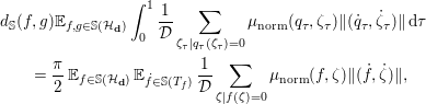 $$\begin{eqnarray}\displaystyle & & \displaystyle d_{\mathbb{S}}(f,g)\mathbb{E}_{f,g\in \mathbb{S}({\mathcal{H}}_{\mathbf{d}})}\int _{0}^{1}\frac{1}{{\mathcal{D}}}\mathop{\sum }_{{\it\zeta}_{{\it\tau}}\mid q_{{\it\tau}}({\it\zeta}_{{\it\tau}})=0}{\it\mu}_{\text{norm}}(q_{{\it\tau}},{\it\zeta}_{{\it\tau}})\Vert (\dot{q}_{{\it\tau}},\dot{{\it\zeta}}_{{\it\tau}})\Vert \,\text{d}{\it\tau}\nonumber\\ \displaystyle & & \displaystyle \qquad =\frac{{\it\pi}}{2}\,\mathbb{E}_{f\in \mathbb{S}({\mathcal{H}}_{\mathbf{d}})}\,\mathbb{E}_{{\dot{f}}\in \mathbb{S}(T_{f})}\,\frac{1}{{\mathcal{D}}}\mathop{\sum }_{{\it\zeta}\mid f({\it\zeta})=0}{\it\mu}_{\text{norm}}(f,{\it\zeta})\Vert ({\dot{f}},\dot{{\it\zeta}})\Vert ,\nonumber\end{eqnarray}$$
where both spheres are endowed with the uniform distribution. It is this uniformity on  $\mathbb{S}(T_{f})$ which allows one, for a fixed
 $f\in {\mathcal{H}}_{\mathbf{d}}$ and
 ${\it\zeta}\in \mathbb{P}^{n}$ with
 $f({\it\zeta})=0$, to look at
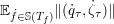 $\mathbb{E}_{{\dot{f}}\in \mathbb{S}(T_{f})}\Vert (\dot{q}_{{\it\tau}},\dot{{\it\zeta}}_{{\it\tau}})\Vert$ as the stochastic condition number of the pair
 $(f,{\it\zeta})$ and use the techniques in Armentano (Reference Armentano2010) to estimate this expectation. This estimate, together with Theorem 3.40 (with
 $\overline{q}=0$ and
 ${\it\sigma}=1$) are finally combined to prove the following improvement to Theorem 3.41.
Theorem 3.45. Algorithm  $\mathsf{LV}$ (with the modified homotopy routine) returns an approximate zero of its input
 $f$ almost surely. Its expected cost is bounded by
 $O(D^{3/2}nN^{3/2})$.◻
3.9 The eigenvalue problem
The second example we want to mention – of a homotopy method for which complexity estimates are obtained via a probabilistic analysis of condition numbers – has to do with the computation of eigenpairs (i.e. eigenvalue–eigenvector pairs) for complex matrices.
The state of the art for the problem was, until very recently, lacunary in the sense that the existing algorithms were either well understood regarding complexity but numerically unstable in practice or they exhibited stable behaviour but defied complexity analysis. The best-known example of the former is that of computing the characteristic polynomial  ${\it\chi}_{A}$ of the
 $n\times n$ input matrix
 $A$ and then approximating the zeros
 ${\it\lambda}_{1},\ldots ,{\it\lambda}_{n}$ of
 ${\it\chi}_{A}$. Both ingredients are known to have low complexity but the whole procedure often fails due to numerical instability. A perfect example of the latter (and today’s algorithm of choice in practice) is the QR iteration with implicit shifts, about which Jim Demmel (Reference Demmel1997, p. 139) wrote:
It is interesting that after more than 30 years of dependable service, convergence failures of this algorithm have quite recently been observed, analysed, and patched … But there is still no global convergence proof, even though the current algorithm is considered quite reliable. So the problem of devising an algorithm that is numerically stable and globally (and quickly!) convergent remains open.
An answer to this demand was very recently given in Armentano et al. (Reference Armentano, Beltrán, Bürgisser, Cucker and Shub2015b), where a homotopy method for computing eigenpairs is analysed and shown to have polynomial-time complexity on average. Homotopy methods had already been considered for eigenvalue problems (see e.g. Li and Sauer Reference Li and Sauer1987) but these previous works did not provide any form of complexity analysis.
We give one final remark before proceeding with the technical core of this example. Since the eigenpair problem has an algebraic nature, one may wonder whether the algorithms for zero finding in the previous example can be applied. Indeed, if we let  $a_{i}$ denote the rows of matrix
 $A$, the equality
 $Av={\it\lambda}v$ can be written as
 $n$ quadratic equations
 $a_{i}v-{\it\lambda}v_{i}=0$,
 $i=1,\ldots ,n$, and we may add the extra equation
 $v_{1}^{2}+\ldots +v_{n}^{2}=1$ ensuring that
 $v\neq 0$. We thus have a system of
 $n+1$ equations in
 $n+1$ variables which, once homogenized, could be considered as an input for algorithm
 $\mathsf{LV}$, for example. Unfortunately, though, with high probability, the execution will loop forever. The reason is that, generically, a system of
 $n+1$ quadratic equations has
 $2^{n+1}$ solutions. In our case,
 $n$ of these are the eigenpairs we are looking for and the remaining
 $2^{n-1}-n$ are ill-posed zeros at infinity (i.e. with
 ${\it\lambda}=\infty$). Following a path corresponding to one of the latter will take infinite time.
(a) The setting.
Given a matrix  $A\in \mathbb{C}^{n\times n}$, we want to compute an eigenpair of
 $A$, that is, a pair
 $({\it\lambda},v)\in \mathbb{C}\times (\mathbb{C}^{n}\setminus \{0\})$ such that
 $Av={\it\lambda}v$. Clearly, if
 $({\it\lambda},v)$ is such a pair then, for all
 $c\in \mathbb{C}\setminus \{0\}$, the pair
 $({\it\lambda},cv)$ is also an eigenpair of
 $A$. Therefore we consider eigenpairs in the product
 $\mathbb{C}\times \mathbb{P}(\mathbb{C}^{n})$. A matrix
 $A\in \mathbb{C}^{n\times n}$ has, generically,
 $n$ different eigenpairs in this product space.
The space  $\mathbb{C}^{n\times n}\times \mathbb{C}\times \mathbb{P}(\mathbb{C}^{n})$ is endowed with the Riemannian product structure. The resulting distance equals
 $$\begin{eqnarray}\mathsf{dist}((A,{\it\lambda},v),(A^{\prime },{\it\lambda}^{\prime },v^{\prime }))^{2}:=\Vert A-A^{\prime }\Vert _{F}^{2}+|{\it\lambda}-{\it\lambda}^{\prime }|^{2}+d_{\mathbb{ P}}(v,v^{\prime })^{2}.\end{eqnarray}$$
We will only use this distance on  $\mathbb{S}\times \mathbb{C}\times \mathbb{P}(\mathbb{C}^{n})$. Note that for
 $A,A^{\prime }\in \mathbb{S}$, the distance
 $\mathsf{dist}((A,{\it\lambda},v),(A^{\prime },{\it\lambda}^{\prime },v^{\prime }))$ is smaller than or equal to the natural geodesic (product) distance in
 $\mathbb{S}\times \mathbb{C}\times \mathbb{P}(\mathbb{C}^{n})$. For any non-zero matrix
 $A\in \mathbb{C}^{n\times n}$ (not necessarily of unit norm) we will write
 $$\begin{eqnarray}\mathsf{dist}_{A}(({\it\lambda},v),({\it\lambda}^{\prime },v^{\prime }))^{2}:=\frac{|{\it\lambda}-{\it\lambda}^{\prime }|^{2}}{\Vert A\Vert _{F}^{2}}+d_{\mathbb{P}}(v,v^{\prime })^{2}.\end{eqnarray}$$
Note that for any non-zero  $A\in \mathbb{C}^{n\times n}$,
 $\mathsf{dist}_{A}$ is a distance function in
 $\mathbb{C}\times \mathbb{P}(\mathbb{C}^{n})$ and if
 $A\in \mathbb{S}$, then
 $$\begin{eqnarray}\mathsf{dist}_{A}(({\it\lambda},v),({\it\lambda}^{\prime },v^{\prime }))=\mathsf{dist}((A,{\it\lambda},v),(A,{\it\lambda}^{\prime },v^{\prime })).\end{eqnarray}$$
A number of notions are defined as in the previous example. Thus we consider the solution manifold
 $$\begin{eqnarray}V=V_{n}:=\{(A,{\it\lambda},v)\in \mathbb{C}^{n\times n}\times \mathbb{C}\times \mathbb{P}(\mathbb{C}^{n})\mid (A-{\it\lambda}\,\text{Id})v=0\},\end{eqnarray}$$
with its natural projections
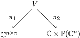
as well as the set  ${\rm\Sigma}^{\prime }$of ill-posed triples
 $(A,{\it\lambda},v)\in V$ for which
 $D{\it\pi}_{1}(A,{\it\lambda},v)$ is not an isomorphism, and the set
 ${\rm\Sigma}:={\it\pi}_{1}({\rm\Sigma}^{\prime })$ of ill-posed matrices.
For  $v\in \mathbb{P}(\mathbb{C}^{n})$ we let
 $v^{\bot }=\{x\in \mathbb{C}^{n}\mid \langle x,v\rangle =0\}$ denote the tangent space to
 $\mathbb{P}(\mathbb{C}^{n})$ at
 $v$. Let
 $P_{v^{\bot }}:\mathbb{C}^{n}\rightarrow v^{\bot }$ be the orthogonal projection. Given
 $(A,{\it\lambda},v)\in \mathbb{C}^{n\times n}\times \mathbb{C}\times \mathbb{P}(\mathbb{C}^{n})$, we let
 $A_{{\it\lambda},v}:v^{\bot }\rightarrow v^{\bot }$ be the linear operator given by
 $$\begin{eqnarray}A_{{\it\lambda},v}:=P_{v^{\bot }}\circ (A-{\it\lambda}\,\text{Id})|_{v^{\bot }}.\end{eqnarray}$$
One can then prove (Armentano Reference Armentano2014, Lemma 2.7) that a triple  $(A,{\it\lambda},v)\in V$ is well-posed if and only if
 $A_{{\it\lambda},v}$ is invertible, which occurs if and only if
 ${\it\lambda}$ is a single eigenvalue of
 $A$.
One can also devise, for a non-zero matrix  $A\in \mathbb{C}^{n\times n}$, a Newton map
 $N_{A}:\mathbb{C}\times \mathbb{P}(\mathbb{C}^{n})\rightarrow \mathbb{C}\times \mathbb{P}(\mathbb{C}^{n})$ associated with
 $A$ by
 $$\begin{eqnarray}N_{A}\binom{{\it\lambda}}{v}=\binom{{\it\lambda}}{v}-\binom{\dot{{\it\lambda}}}{\dot{v}},\quad \text{where }\binom{\dot{{\it\lambda}}}{\dot{v}}=(DF_{A}({\it\lambda},v)\mid _{\mathbb{C}\times v^{\bot }})^{-1}F_{A}\binom{{\it\lambda}}{v}\end{eqnarray}$$
and  $F_{A}({\it\lambda},v)=(A-{\it\lambda}\,\text{Id})v$ is the evaluation map. This map was introduced in Armentano (Reference Armentano2014) as a Newton-like operator associated with the evaluation map
 $F_{A}$, and the following formulas were obtained for
 $\dot{v}$ and
 $\dot{{\it\lambda}}$ (recall the definition of
 $A_{{\it\lambda},v}$ from (3.33)):
 $$\begin{eqnarray}\dot{v}={A_{{\it\lambda},v}}^{-1}\,P_{v^{\bot }}Av,\quad \dot{{\it\lambda}}=\frac{\langle ({\it\lambda}\,\text{Id}-A)(v-\dot{v}),v\rangle }{\langle v,v\rangle }.\end{eqnarray}$$
It is immediate to see that  $N_{A}({\it\lambda},v)$ does not depend on the representative in
 $\mathbb{C}^{n}\setminus \{0\}$ for
 $v\in \mathbb{P}(\mathbb{C}^{n})$. We also note that
 $N_{A}({\it\zeta},w)$ can be computed from the matrix
 $A$ and the pair
 $({\it\zeta},w)$ in
 $O(n^{3})$ operations, since the cost of this computation is dominated by that of inverting a matrix (or simply solving a linear system).
With Newton’s algorithm at our disposal the following definition is natural.
Definition 3.46. Given  $(A,{\it\lambda},v)\in V\setminus {\rm\Sigma}^{\prime }$ we say that
 $({\it\zeta},w)\in \mathbb{C}\times \mathbb{P}(\mathbb{C}^{n})$ is an approximate eigenpair of
 $A$ with associated eigenpair
 $({\it\lambda},v)$ when, for all
 $k\geq 1$, the
 $k$th iterate
 $N_{A}^{k}({\it\zeta},w)$ of the Newton map at
 $({\it\zeta},w)$ is well defined and satisfies
 $$\begin{eqnarray}\mathsf{dist}_{A}((N_{A}^{k}({\it\zeta},w)),({\it\lambda},v))\leq \biggl(\frac{1}{2}\biggr)^{2^{k}-1}\mathsf{dist}_{A}(({\it\zeta},w),({\it\lambda},v)).\end{eqnarray}$$
The following result (for a proof see Armentano Reference Armentano2014, Theorem 5) is a version of Theorem 3.38.
Theorem 3.47. There is a constant  $c_{0}>1/5$ with the following property. Let
 $(A,{\it\lambda},v)\in V\setminus {\rm\Sigma}^{\prime }$ with
 $\Vert A\Vert _{F}=1$ and let
 $({\it\zeta},w)\in \mathbb{C}\times \mathbb{P}(\mathbb{C}^{n})$. If
 $$\begin{eqnarray}\mathsf{dist}_{A}(({\it\lambda},v),({\it\zeta},w))\leq \frac{c_{0}}{{\it\mu}(A,{\it\lambda},v)},\end{eqnarray}$$
then  $({\it\zeta},w)$ is an approximate eigenpair of
 $A$ with associated eigenpair
 $({\it\lambda},v)$.◻
(b) Condition numbers.
The framework we described in Section 1.1(b) along with the projections
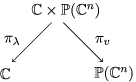
allow us to define two condition numbers for eigenvalue and eigenvector, respectively. Formulas for both of them have been known at least since Van Loan (Reference Van Loan1987). Armentano (Reference Armentano2014, § 3) has shown that one can merge the two, which, with minor changes, leads to the definition of the condition number of  $(A,{\it\lambda},v)\in \mathbb{C}^{n\times n}\times \mathbb{C}\times \mathbb{P}(\mathbb{C}^{n})$ in Armentano et al. (Reference Armentano, Beltrán, Bürgisser, Cucker and Shub2015b), namely
 $$\begin{eqnarray}{\it\mu}(A,{\it\lambda},v):=\Vert A\Vert _{F}\Vert A_{{\it\lambda},v}^{-1}\Vert ,\end{eqnarray}$$
(or  $\infty$ if
 $A_{{\it\lambda},v}$ is not invertible) where
 $\Vert \cdot \Vert$ is the operator norm. This coincides with
 ${\it\mu}_{v}(A,{\it\lambda},v)$ in Armentano (Reference Armentano2014). When restricted to the class of normal matrices, the condition number
 ${\it\mu}$ admits the following elegant characterization.
Lemma 3.48 (Armentano Reference Armentano2014, Lemma 3.12).
Let  $A\in \mathbb{C}^{n\times n}\setminus {\rm\Sigma}$ be normal, and let
 $({\it\lambda}_{1},v_{1}),\ldots ,({\it\lambda}_{n},v_{n})$ be its eigenpairs. Then
 $$\begin{eqnarray}{\it\mu}(A,{\it\lambda}_{1},v_{1})=\frac{\Vert A\Vert _{F}}{\min _{j=2,\ldots ,n}|{\it\lambda}_{j}-{\it\lambda}_{1}|}.\square\end{eqnarray}$$
As in the case of polynomial systems, we can define the the mean square condition number of  $A$ by
 $$\begin{eqnarray}{\it\mu}_{\mathsf{av}}^{2}(A):=\frac{1}{n}\mathop{\sum }_{j=1}^{n}{\it\mu}^{2}(A,{\it\lambda}_{j},v_{j}).\end{eqnarray}$$
The version for the eigenpair problem of Theorem 3.40 is as follows (see Armentano et al. Reference Armentano, Beltrán, Bürgisser, Cucker and Shub2015b, Theorem 2.14).
Theorem 3.49. For  $\overline{A}\in \mathbb{C}^{n\times n}$ and
 ${\it\sigma}>0$ we have
 $$\begin{eqnarray}\mathbb{E}_{A\sim N(\overline{A},{\it\sigma}^{2}\text{Id})}\biggl(\frac{{\it\mu}_{\mathsf{av}}^{2}(A)}{\Vert A\Vert _{F}^{2}}\biggr)\leq \frac{n}{{\it\sigma}^{2}}.\square\end{eqnarray}$$
(c) Complexity results: deterministic algorithms.
Theorems 3.47 and 3.49 allow us to follow the main reasoning in the previous example to design and analyse homotopy algorithms for the eigenpair problem. Indeed, as in the previous example, one can take the step-length in the homotopy to be proportional to the inverse of  ${\it\mu}^{2}(B_{i},{\it\zeta}_{i},w_{i})$, where
 $B_{i}$ is the matrix dealt with at the
 $i$th iteration and
 $({\it\zeta}_{i},w_{i})$ is an approximate eigenpair of
 $B_{i}$. A result like Theorem 3.39 (without the
 $D^{3/2}$ factor) likewise follows, and an appropriate choice of initial triples leads to the following two results (for computing one or all of the eigenpairs of a matrix).
Theorem 3.50 (Armentano et al. Reference Armentano, Beltrán, Bürgisser, Cucker and Shub2015b, Theorem 2.24).
There exists a homotopy algorithm Single_Eigenpair which returns (almost surely) an approximate eigenpair of its input  $A\in \mathbb{C}^{n\times n}$. Its average cost is bounded by
 $O(n^{7})$.◻
Theorem 3.51 (Armentano et al. Reference Armentano, Beltrán, Bürgisser, Cucker and Shub2015b, Theorem 2.27).
There exists a homotopy algorithm All_Eigenpairs which returns (almost surely)  $n$ approximate eigenpairs of its input
 $A\in \mathbb{C}^{n\times n}$ with pairwise different associated eigenpairs. Its average cost is bounded by
 $O(n^{9})$.◻
(d) Complexity results: randomized algorithms.
The ideas described in Section 3.8(g) can be used in the context of the eigenpair problem. A modification to the computation of the step-length of the homotopy leads to the following result (Armentano et al. Reference Armentano, Beltrán, Bürgisser, Cucker and Shub2015b, Theorem 2.28).
Proposition 3.52. The expected (with respect to both the input matrix  $A$ and the initial triple
 $(A_{0},{\it\lambda}_{0},v_{0})$) number of homotopy steps satisfies
 $$\begin{eqnarray}\mathbb{E}_{A\sim N(0,\text{Id})}\mathbb{E}_{A_{0}\sim N(0,\text{Id})}\;\frac{1}{n}\mathop{\sum }_{({\it\lambda}_{0},v_{0})\mid (A_{0},{\it\lambda}_{0},v_{0})\in V}K(A,A_{0},{\it\lambda}_{0},v_{0})\leq Cn^{2},\end{eqnarray}$$
where  $C$ is a universal constant.◻
If we had a procedure to efficiently draw triples from the distribution in  $V$ informally described by
 $$\begin{eqnarray}\displaystyle & & \displaystyle \mathtt{randomly~choose}~A_{0}\sim N(0,\text{Id})\nonumber\\ \displaystyle & & \displaystyle \mathtt{randomly~choose~one~eigenpair}~({\it\lambda}_{0},v_{0})~\mathtt{of}~A_{0}\nonumber\end{eqnarray}$$
we could design a Las Vegas algorithm like the one in the previous example, computing a single eigenpair of its input matrix in average randomized time  $O(n^{5})$ (since each iteration of the homotopy has a cost of
 $O(n^{3})$). As it happens, we do not have such a procedure. Nonetheless, a randomized algorithm can be designed whose analysis takes advantage of Proposition 3.52. This analysis, however, has an overhead cost that eventually leads to an average randomized cost of
 $O(n^{7})$ (Armentano et al. Reference Armentano, Beltrán, Bürgisser, Cucker and Shub2015b, Theorem 2.34).
3.10 General bounds for conic condition numbers
The last example in this repertoire is not, strictly speaking, an example but rather a general result from which many examples can be derived.
Recall that at the beginning of Section 2 we defined conic condition numbers as those that admit an expression of the form
 $$\begin{eqnarray}\mathscr{C}(a):=\frac{\Vert a\Vert }{\mathsf{dist}(a,{\rm\Sigma})}.\end{eqnarray}$$
In what follows we assume that the data  $a\in \mathbb{K}^{p+1}$ where
 $\mathbb{K}$ is
 $\mathbb{R}$ or
 $\mathbb{C}$ and that the norm and distance above are induced by an inner (resp. Hermitian) product. We also assume that the set
 ${\rm\Sigma}$ of ill-posed instances is an algebraic cone in
 $\mathbb{K}^{p+1}$, that is, a Zariski closed subset that is closed under multiplication by elements in
 $\mathbb{K}$. The main contention of Demmel (Reference Demmel1987) is that many (if not most) of the condition numbers we associate with a variety of problems are – or are closely approximated by – a conic condition number as above.
The fact that  ${\rm\Sigma}$ is a cone implies that for all
 $a\in \mathbb{K}^{p+1}$ and all
 ${\it\lambda}\in \mathbb{K}\setminus \{0\}$ we have
 $\mathscr{C}(a)=\mathscr{C}({\it\lambda}a)$. Hence, we may restrict attention to data
 $a\in \mathbb{P}^{p}:=\mathbb{P}(\mathbb{K}^{p+1})$ in projective space over
 $\mathbb{K}$ for which the condition number takes the form
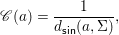 $$\begin{eqnarray}\mathscr{C}(a)=\frac{1}{d_{\mathsf{sin}}(a,{\rm\Sigma})},\end{eqnarray}$$
where, abusing notation,  ${\rm\Sigma}$ is interpreted now as a subset of
 $\mathbb{P}^{p}$ and
 $d_{\mathsf{sin}}=\sin d_{\mathbb{P}}$ denotes the sine distance in
 $\mathbb{P}^{p}$ (see Figure 3.4).
Three distances.
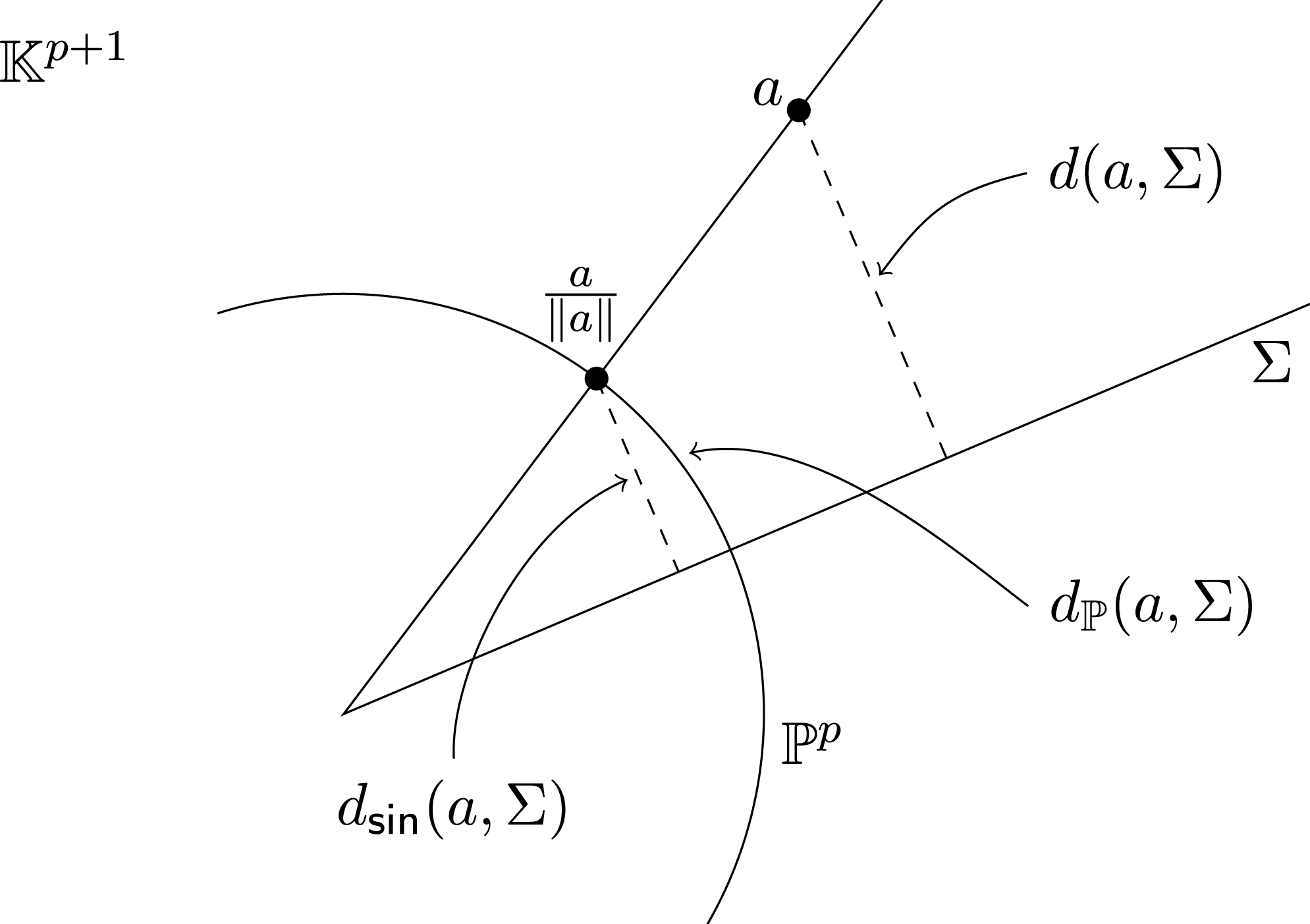
Because  ${\rm\Sigma}$ is a projective variety, it has associated with it a number of geometric invariants, notably a dimension
 $m=\dim _{\mathbb{K}}{\rm\Sigma}$ and a degree
 $d=\mathsf{deg}{\rm\Sigma}$.
In a sequel to his Reference Demmel1987 paper, Jim Demmel (Reference Demmel1988) endowed projective space  $\mathbb{P}^{p}$ with the uniform distribution and exhibited bounds for the probability tail of
 $\mathscr{C}$ depending only on the parameters
 $p$,
 $m$ and
 $d$. Estimates for the expectation of
 $\mathscr{C}$ or of
 $\log \mathscr{C}$ (also depending on these parameters) follow from these bounds using well-known arguments. This average analysis was extended to a smoothed analysis in Bürgisser, Cucker and Lotz (Reference Bürgisser, Cucker and Lotz2006, Reference Bürgisser, Cucker and Lotz2008) but, unlike the previous examples, not for Gaussian perturbations but for perturbations uniformly chosen on balls in projective space.
Since the total volume of  $\mathbb{P}^{p}$ for its Riemannian measure is finite, it makes sense to talk about the uniform probability distribution on the closed ball
 $B(\overline{a},{\it\sigma})$ of radius
 ${\it\sigma}$ around
 $\overline{a}\in \mathbb{P}^{p}$ with respect to
 $d_{\mathsf{sin}}$. We thus consider a smoothed analysis of
 $\mathscr{C}$ whereby a random perturbation
 $a$ of
 $\overline{a}\in \mathbb{P}^{p}$ is modelled by choosing
 $a\in B(\overline{a},{\it\sigma})$ from the uniform distribution on
 $B(\overline{a},{\it\sigma})$.
The case  $\mathbb{K}=\mathbb{C}$ allows for a very general result, the only restriction being that the set of ill-posed inputs
 ${\rm\Sigma}$ is purely dimensional, that is, all of its irreducible components have the same dimension. This is almost invariably the case for common computational problems. The version of this result in Bürgisser and Cucker (Reference Bürgisser and Cucker2013, Theorem 20.1) reads as follows.
Theorem 3.53. Let  $\mathscr{C}$ be a conic condition number with a set of ill-posed inputs
 ${\rm\Sigma}\subseteq \mathbb{P}(\mathbb{C}^{p+1})$, of pure dimension
 $m$,
 $0<m<p$. Let
 $$\begin{eqnarray}K(p,m):=2\frac{p^{3p}}{m^{3m}(p-m)^{3(p-m)}}.\end{eqnarray}$$
Then, for all  $\overline{a}\in \mathbb{P}(\mathbb{C}^{p+1})$, all
 ${\it\sigma}\in (0,1]$, and all
 $$\begin{eqnarray}t\geq \frac{p\sqrt{2m}}{p-m},\end{eqnarray}$$
we have
 $$\begin{eqnarray}\underset{a\in B(\overline{a},{\it\sigma})}{\mathsf{Prob}}\{\mathscr{C}(a)\geq t\}\leq K(p,m)\,\mathsf{deg}{\rm\Sigma}\biggl(\frac{1}{t{\it\sigma}}\biggr)^{2(p-m)}\biggl(1+\frac{p}{p-m}\frac{1}{t{\it\sigma}}\biggr)^{2m},\end{eqnarray}$$
as well as
 $$\begin{eqnarray}\mathbb{E}_{a\in B(\overline{a},{\it\sigma})}(\mathscr{C}(a))\leq 2eK(p,m)^{\frac{1}{2(p-m)}}\,(\mathsf{deg}{\rm\Sigma})^{\frac{1}{2(p-m)}}\,\frac{pm}{p-m}\,\frac{1}{{\it\sigma}}\end{eqnarray}$$
and
 $$\begin{eqnarray}\displaystyle & & \displaystyle \mathbb{E}_{a\in B(\overline{a},{\it\sigma})}(\log \mathscr{C}(a))\nonumber\\ \displaystyle & & \displaystyle \qquad \leq \frac{1}{2(p-m)}(\log K(p,m)+\log \mathsf{deg}{\rm\Sigma}+3\log e)+\log \frac{pm}{p-m}+\log \frac{1}{{\it\sigma}}.\nonumber\end{eqnarray}$$
Taking  ${\it\sigma}=1$, we obtain an average-case analysis. ◻
In most applications, the set of ill-posed inputs  ${\rm\Sigma}$ is a hypersurface. That is,
 ${\rm\Sigma}$ is the zero set
 $Z_{\mathbb{P}}(f)$ of a non-zero homogeneous polynomial
 $f$, and thus
 $\mathsf{deg}{\rm\Sigma}$ is at most the degree of
 $f$. In this case, we have the following corollary.
Corollary 3.54. Let  $\mathscr{C}$ be a conic condition number with set of ill-posed inputs
 ${\rm\Sigma}\subseteq \mathbb{P}(\mathbb{C}^{p+1})$. Assume
 ${\rm\Sigma}\subseteq Z_{\mathbb{P}}(f)$ with
 $f\in \mathbb{C}[X_{0},\ldots ,X_{p}]$ homogeneous of degree
 $d$. Then, for all
 $\overline{a}\in \mathbb{P}(\mathbb{C}^{p+1})$, all
 ${\it\sigma}\in (0,1]$, and all
 $t\geq \sqrt{2}\,p^{3/2}$,
 $$\begin{eqnarray}\underset{a\in B(\overline{a},{\it\sigma})}{\mathsf{Prob}}\{\mathscr{C}(a)\geq t\}\leq 2e^{3}p^{3}d\biggl(\frac{1}{t{\it\sigma}}\biggr)^{2}\biggl(1+p\frac{1}{t{\it\sigma}}\biggr)^{2(p-1)}\end{eqnarray}$$
as well as
 $$\begin{eqnarray}\mathbb{E}_{a\in B(\overline{a},{\it\sigma})}(\mathscr{C}(a))\leq 4(2e^{5})^{1/2}p^{3/2}\,d^{1/2}\,\frac{1}{{\it\sigma}}\end{eqnarray}$$
and
 $$\begin{eqnarray}\mathbb{E}_{a\in B(\overline{a},{\it\sigma})}(\log \mathscr{C}(a))\leq \frac{3}{2}\log p+\frac{1}{2}\log d+\log \frac{1}{{\it\sigma}}+3\log e+\frac{3}{2}.\end{eqnarray}$$
Taking  ${\it\sigma}=1$, one obtains an average-case analysis. ◻
The case  $\mathbb{K}=\mathbb{R}$ turns out to be more complicated. Demmel (Reference Demmel1988) states a result which he attributed to Adrian Ocneanu, estimating the volume of
 ${\it\varepsilon}$-tubes around real algebraic varieties, and makes a conjecture on the asymptotic behaviour of these volumes when
 ${\it\varepsilon}$ tends to zero. Ocneanu’s result, however, is cited as an unpublished report and, as of today, it remains so. Very recently, Martin Lotz (Reference Lotz2015) gave a proof of this result and, in passing, proved Demmel’s conjecture. But he did not derive a probabilistic analysis for conic condition numbers. Moreover, as well as the condition on pure dimensionality assumed in the complex case, these results impose a more stringent requirement, namely that the real algebraic variety is a complete intersection.
The general bound in Bürgisser, Cucker and Lotz (Reference Bürgisser, Cucker and Lotz2008) (which we cite again from the more recent version in Bürgisser and Cucker Reference Bürgisser and Cucker2013) is weaker than its complex counterpart.
Theorem 3.55. Let  $\mathscr{C}$ be a conic condition number with a set of ill-posed inputs
 ${\rm\Sigma}$. Assume that
 ${\rm\Sigma}$ is contained in a real algebraic hypersurface, given as the zero set of a homogeneous polynomial of degree
 $d$. Then, for all
 $0<{\it\sigma}\leq 1$ and all
 $t\geq (2d+1)(p/{\it\sigma})$, we have
 $$\begin{eqnarray}\sup _{\overline{a}\in \mathbb{S}^{p}}~\underset{a\in B_{\mathsf{sin}}(\overline{a},{\it\sigma})}{\mathsf{Prob}}\{\mathscr{C}(a)\geq t\}\leq 4e\,\text{d}p\,\frac{1}{{\it\sigma}t}\end{eqnarray}$$
and
 $$\begin{eqnarray}\sup _{\overline{a}\in \mathbb{S}^{p}}\,\mathbb{E}_{a\in B_{\mathsf{sin}}(\overline{a},{\it\sigma})}\log \mathscr{C}(a)\leq \log p+\log d+\log \frac{1}{{\it\sigma}}+\log (4e^{2}).\end{eqnarray}$$
In particular (take  ${\it\sigma}=1$), for all
 $t\geq (2d+1)p$,
 $$\begin{eqnarray}\underset{a\in \mathbb{S}^{p}}{\mathsf{Prob}}\{\mathscr{C}(a)\geq t\}\leq 4e\,\text{d}p\,\frac{1}{t}\end{eqnarray}$$
and
 $$\begin{eqnarray}\mathbb{E}_{a\in \mathbb{S}^{p}}(\log \mathscr{C}(a))\leq \log p+\log d+\log (4e^{2}).\square\end{eqnarray}$$
Very likely, one can extend Theorem 3.55 to obtain probability tails with a rate of decay of the order of  $t^{p-m}$ in the case when
 ${\rm\Sigma}$ is a complete intersection, by adapting the results in Lotz (Reference Lotz2015).