





1. Introduction
Let
 $p\in\mathbb{N}$
be fixed, and let
 $\boldsymbol{\xi} = (\xi^{i,j})_{i,j=1,\ldots,p}$
be an arbitrary matrix of point processes on the nonnegative half-line. For a given law of
 $\boldsymbol{\xi}$
, there is a natural way to construct a multi-type branching process whose evolution is governed by
 $\boldsymbol{\xi}$
. Initially, there is a single individual of type
 $i\in\{1,\dots,p\}$
. This individual gives birth to children of various types at different times. More precisely, for
 $j\in\{1,\dots,p\}$
, the atoms of
 $\xi^{i,j}$
give the ages of the parent at which it gives birth to offspring of type j; that is, at age t, it gives birth to
 $\xi^{i,j}(\{t\})$
children of type j. Each newly born individual evolves independently according to the same dynamics, with its own independent copy of
 $\boldsymbol{\xi}$
.
This model encompasses many classical branching models. For example, it reduces to a Galton–Watson process when all point processes are supported on the single point
 $\{1\}$
, to a continuous-time Markov branching process when the measures are supported on a single point given by an exponential random variable independent of the number of offspring, and to a Bellman–Harris branching process when the supporting point follows a more general distribution. We refer to [Reference Jagers9] for a detailed introduction to the theory of single-type Crump–Mode–Jagers (CMJ) processes, to [Reference Iksanov and Meiners8] for an introduction to the theory with a finite type space, and to [Reference Jagers10] for an introduction to the theory with an abstract type space.
Denote by
 $\mathcal{Z}_t^j$
the number of type-j individuals alive at time
 $t \geq 0$
. If there exists a Malthusian parameter
 $\alpha \gt 0$
, then
 $\mathrm{e}^{-\alpha t}\mathcal{Z}_t^j$
converges to a random limit; see, e.g., [Reference Iksanov and Meiners8, Reference Nerman14]. More precisely, let
 $\mathcal{C}_t$
denote the set of individuals who are the first in their line of descent to be born strictly after time t. For
 $u\in \mathcal{C}_t$
, let S(u) and
 $\tau(u)$
denote the birth time and type of individual u, respectively. Then there exists a vector
 $v=(v_1,\dots, v_p)$
such that
 \begin{align*} W_t(\alpha) = \sum_{u \in \mathcal{C}_t} \frac{v_{\tau(u)}}{v_i}\mathrm{e}^{-\alpha S(u)}, \quad t \geq 0,\end{align*}
defines a nonnegative martingale
 $(W_t(\alpha))_{t \geq 0}$
, known as Nerman’s martingale, which converges almost surely to some nonnegative random variable
 $W(\alpha)$
. The convergence holds in
 $L^1$
under an additional
 $L\log L$
condition; see, e.g., [Reference Iksanov and Meiners8, Reference Kyprianou and Rahimzadeh Sani12, Reference Nerman14]. Moreover, almost surely,
 $\mathrm{e}^{-\alpha t} \mathcal{Z}_t^j \to c_{i,j} W(\alpha)$
as
 $t \to \infty$
, where
 $c_{i,j} \gt 0$
is a constant depending on the initial type i and the target type j; see, for instance, [Reference Iksanov and Meiners8, Reference Nerman14].
The processes
 $\mathcal{Z}_t^j$
are among the most important examples of CMJ processes; see [Reference Iksanov and Meiners8, Reference Jagers9] for precise definitions. The convergence above is known as a strong law of large numbers for these processes. A natural question is whether this strong law of large numbers is accompanied by a central limit theorem. An affirmative answer has been obtained in several particular models.
In the single-type case, i.e. when
 $p=1$
, the process
 $\mathcal{Z}^1_t$
represents the total number of individuals ever born. It turns out that, between the leading term
 $\mathrm{e}^{\alpha t} W(\alpha)$
and the Gaussian fluctuations of the exponential order of magnitude
 $\mathrm{e}^{\alpha t/2}$
, there can be additional subleading terms of the form
 $\mathrm{e}^{\lambda t}t^{k}W^{(l)}(\lambda)$
, where
 $\lambda$
ranges over the roots of the equation
 \begin{align*} \int \mathrm{e}^{\lambda x} \,\mathbb{E}[\xi](\mathrm{d} \mathit{x})=1\end{align*}
lying in the half-plane
 $\{\operatorname{Re}(z)\gt\alpha/2\}$
, and l is smaller than the multiplicity of the root
 $\lambda$
. The process
 $W_t^{(l)}(\lambda) = \sum_{u \in \mathcal{C}_t} S(u)^l \mathrm{e}^{-\lambda S(u)}$
,
 $t\ge0$
, is also a martingale, with limit
 $W^{(l)}(\lambda)$
whenever it converges. Then, for suitable constants
 $c_{\lambda,k,l}$
, the difference
 \begin{align} \mathcal{Z}^1_t - c\mathrm{e}^{\alpha t}W(\alpha) - \sum_{\lambda,k,l}c_{\lambda,k,l}\mathrm{e}^{\lambda t}t^{k}W^{(l)}(\lambda)\end{align}
converges, after appropriate normalization, to a normal distribution, typically with a random variance; see [Reference Iksanov, Kolesko and Meiners7].
Note that, for
 $l=0$
, the martingale above is closely related to the well-known additive martingale [Reference Biggins2, Reference Lyons13] also called Biggins’ martingale. It is worth mentioning that the limits of the two martingales coincide [Reference Gatzouras3, Theorem 3.3]. When
 $l=1$
, the corresponding object is an analog of the derivative martingale. Both Biggins’ additive martingale and the derivative martingale are usually defined for branching random walks, where the positions S(u) may take negative values. This is not possible in the present setting.
The multi-type case, that is, when
 $p\gt1$
, is much less understood. In the special case where
 $\mathcal{Z}_t=(\mathcal{Z}^1_t,\dots,\mathcal{Z}^p_t)$
is a multi-type continuous-time Markov branching process, the expectation
 $\mathbb{E} [\mathcal{Z}(t)]$
is given by a semigroup,
 $\mathbb{E} [\mathcal{Z}_t]=\mathcal{Z}_0\mathrm{e}^{tA}$
,
 $t\ge0$
, where A is a matrix with dominant eigenvalue
 $\alpha$
; see, e.g., [Reference Athreya and Ney1, Chapter V.7]. Then, for any eigenvalue
 $\lambda$
of A, and with
 $P_\lambda$
denoting the spectral projection onto the generalized eigenspace corresponding to
 $\lambda$
, the process
 $W_t(\lambda)=\mathrm{e}^{- t A} P_\lambda \mathcal{Z}_t$
is a vector-valued martingale that converges whenever
 $\operatorname{Re}(\lambda)\gt\alpha/2$
. The components of its limit play the same role as the variables
 $W^{(l)}(\lambda)$
in (1.1) in the single-type setting.
A natural question is whether we can construct martingales in the general multi-type setting that recover all of the examples described above as special cases. The aim of this paper is to provide such a construction, together with conditions ensuring convergence in
 $L^q$
for
 $1\lt q\leq2$
. The most important case with regard to the central limit theorem is the case
 $q=2$
. In a subsequent paper, we will establish an analog of the limit theorem (1.1) for multi-type CMJ processes.
2. Assumptions and main result
We continue by rigorously formulating the model, followed by a precise statement of our main results.
2.1. Model description
In this section, we formally introduce the multi-type general (CMJ) branching process. The process begins with a single individual, the ancestor, born at time 0. It is assigned the label
 $\varnothing$
, the empty tuple, and, like every individual in the process, is of one of finitely many types:
 $\tau(\varnothing) \in [\,p\,] \;:\!=\; \{1, \ldots, p\}$
, where
 $p \in \mathbb{N} = \{1,2,3,\ldots\}$
denotes the number of distinct types. If
 $\tau(\varnothing) = i$
, meaning the ancestor is of type i, then its children of type j are born at the points of the random point process
 $\xi^{i,j}$
, for
 $j = 1, \ldots, p$
. Throughout, we assume that each
 $\xi^{i,j}$
is supported on
 $[0, \infty)$
, and hence its total mass is given by
 $N^{i,j} = \xi^{i,j}([0, \infty))$
. The random variables
 $N^{i,j}$
take values in
 $\mathbb{N}_0 \cup \{\infty\}$
, where
 $\mathbb{N}_0 \;:\!=\; \mathbb{N} \cup \{0\}$
. In particular, we allow for the possibility that
 $\mathbb{P}(N^{i,j} = \infty) \gt 0$
, which means that the ancestor may give rise to an infinite number of children of a given type. We denote by
 $\boldsymbol{\xi} = (\xi^{i,j})_{i,j = 1,\ldots,p}$
the
 $p \times p$
matrix of point processes that determines the reproduction behavior of the ancestor. The individual processes
 $\xi^{i,j}$
are referred to as offspring processes, and the matrix
 $\boldsymbol{\xi}$
as the offspring process matrix.
Throughout this text, we denote by
 ${e}_1, \ldots, {e}_p$
the canonical basis vectors of
 $\mathbb{R}^{1 \times p}$
, considered as row vectors. Using this notation, we express the vector of offspring point processes for an individual of type i as
 $\xi^{i} = \sum_{j=1}^p \xi^{i,j} {e}_j = (\xi^{i,1}, \ldots, \xi^{i,p})$
, which collects, component-wise, the reproduction processes for each offspring type. Similarly, we define the offspring count vector for an individual of type i as
 $N^i \;:\!=\; \sum_{j=1}^p N^{i,j} \, {e}_j$
. We further define
 \begin{align*} \xi(\!\cdot\!) \;:\!=\; \sum_{j=1}^p \xi^{\tau(\varnothing),j}(\!\cdot\!) = \sum_{k=1}^{N} \delta_{X_k}(\!\cdot\!),\end{align*}
where
 $N = \sum_{j=1}^p N^{\tau(\varnothing),j} = \xi([0,\infty))$
is the total number of offspring of the ancestor and
 $\delta_x$
is the Dirac measure with a point at x. The point process
 $\xi$
thus records the birth times of all children of the ancestor, irrespective of their types. Without loss of generality, we assume that
 $0 \leq X_1 \leq X_2 \leq \cdots$
, in which case each birth time
 $X_k$
can be recovered as
 \begin{align*} X_k = \inf\{t \geq 0 \colon \xi([0, t]) \geq k\}, \quad k \in \mathbb{N},\end{align*}
where
 $X_k = \infty$
indicates that the ancestor has strictly fewer than k children.
The multi-type general branching process is then constructed by allowing each child of the ancestor to produce offspring according to an independent copy of the point process matrix
 $\boldsymbol{\xi}$
. These offspring, in turn, reproduce independently according to further independent copies of
 $\boldsymbol{\xi}$
, and so on. To formalize this, we introduce the standard Ulam–Harris notation. Let
 $\mathbb{N}^0 \;:\!=\; \{\varnothing\}$
denote the set containing only the empty tuple. The infinite Ulam–Harris tree is defined as
 \begin{align*} \mathcal{I} \;:\!=\; \bigcup_{n \in \mathbb{N}_0} \mathbb{N}^n,\end{align*}
i.e. the set of all finite sequences (tuples) of natural numbers. We abbreviate elements
 $u = (u_1,\ldots,u_n) \in \mathcal{I}$
by writing
 $u_1\ldots u_n$
. Given another element
 $v = v_1 \ldots v_m \in \mathcal{I}$
, their concatenation is denoted
 $uv = u_1 \ldots u_n v_1 \ldots v_m$
. The Ulam–Harris tree
 $\mathcal{I}$
serves as the set of labels for all potential individuals. Each
 $u \in \mathcal{I}$
identifies a unique individual with ancestral line
 \begin{align*} \varnothing \rightarrow u_1 \rightarrow u_1u_2 \rightarrow \cdots \rightarrow u_1\ldots u_n = u,\end{align*}
where
 $u_1$
is the
 $u_1$
th child of the ancestor,
 $u_1u_2$
the
 $u_2$
th child of
 $u_1$
, and so on. We write
 $|u| = n$
to indicate that u belongs to generation n. For
 $u \in \mathcal{I}$
and
 $i \in \mathbb{N}$
, the label ui corresponds to the ith child of u, and we refer to u as the parent of ui. More generally, we write
 $u \preceq v$
if
 $v = uw$
for some
 $w \in \mathcal{I}$
, and say that u is an ancestor of v, and v is a descendant of u. If, in addition,
 $u \neq v$
, we write
 $u \prec v$
. For
 $u = u_1 \ldots u_n \in \mathcal{I}$
and
 $k \in \mathbb{N}_0$
, we denote by
 $u|_k$
the ancestor of u in generation k if
 $k \leq |u|$
, and
 $u|_k = u$
otherwise.
Let
 $\boldsymbol{\xi}_u=(\xi_u^{i,j})_{i,j = 1,\ldots,p}$
,
 $u \in \mathcal{I} \setminus \{\varnothing\}$
be a family of copies of
 $\boldsymbol{\xi} \;=\!:\; \boldsymbol{\xi}_\varnothing$
. We write
 \begin{align*} \xi_u^{i} = \sum_{j=1}^p \xi_u^{i,j} {e}_j.\end{align*}
Let
 $(\Omega,\mathcal{A},\mathbb{P})$
be a probability space on which all
 $\boldsymbol{\xi}_u$
,
 $u \in \mathcal{I}$
, are defined, and independent and identically distributed (i.i.d.), and independent of
 $\tau(\varnothing)$
, the random variable that gives the ancestor’s type; we write
 $\mathbb{P}^i$
if the ancestor’s type is
 $i \in [\,p\,]$
. We denote the associated expected value operators by
 $\mathbb{E}$
and
 $\mathrm{e}^i$
, respectively.
Generation 0 of the process is given by
 $\mathcal{G}_0 \;:\!=\; \{\varnothing\}$
. The first generation is represented by the random set
 $\mathcal{G}_1 \;:\!=\; \{k \in \mathbb{N} \colon X_k \lt \infty\} \subseteq \mathbb{N}$
, where each
 $k \in \mathcal{G}_1$
is assigned a type
 $\tau(k) \in [\,p\,]$
. Now suppose that generation
 $\mathcal{G}_n$
has been constructed and let
 $u \in \mathcal{G}_n$
be an individual of type
 $\tau(u) \in [\,p\,]$
. Define the point process
 \begin{align*} \xi_u \;:\!=\; \sum_{j=1}^p \xi_u^{\tau(u),j} = \sum_{k=1}^{N_u} \delta_{X_{u,k}},\end{align*}
where
 $N_u = \xi_u([0,\infty))$
is the total number of offspring of u and
 \begin{align*} X_{u,k} = \inf\{t \geq 0 \colon \xi_u([0,t]) \geq k\}, \quad k \in \mathbb{N},\end{align*}
where the infimum of the empty set is set to be
 $\infty$
. Then the
 $(n+1)$
th generation is given by
 \begin{align*} \mathcal{G}_{n+1} \;:\!=\; \{uk \in \mathcal{I} \colon u \in \mathcal{G}_n \text{ and } X_{u,k} \lt \infty\}.\end{align*}
The full population is described by the family tree
 $\mathcal{T} \;:\!=\; \bigcup_{n \in \mathbb{N}_0} \mathcal{G}_n$
. Each
 $u \in \mathcal{T}$
has a type
 $\tau(u) \in [\,p\,]$
and a well-defined birth time
 $S(u) \in [0,\infty)$
, given by
 \begin{align*} S(u) = \sum_{k=1}^n X_{u|_{k-1}, u_k} \quad \text{for } u = u_1 \ldots u_n.\end{align*}
For
 $t \geq 0$
and
 $j \in [\,p\,]$
, define the counting process
 \begin{align*} \mathcal{Z}_t^j \;:\!=\; \sum_{u \in \mathcal{T}} {1}_{\{\,j\}}(\tau(u)) {1}_{[0,\infty)}(t - S(u)),\end{align*}
which counts the number of individuals of type j born up to and including time t. The corresponding vector process is
 $\mathcal{Z}_t \;:\!=\; (\mathcal{Z}_t^1, \ldots, \mathcal{Z}_t^p)$
, and
 $(\mathcal{Z}_t)_{t \geq 0}$
is the multi-type general branching process.
2.2. Assumptions
We define
 $\mu^{i,j} := \mathbb{E}[\xi^{i,j}]$
as the intensity measure of
 $\xi^{i,j}$
for
 $i,j \in [\,p\,]$
, and let
 $\boldsymbol{\mu} \;:\!=\; (\mu^{i,j})_{i,j=1,\ldots,p} = \mathbb{E}[\boldsymbol{\xi}]$
denote the corresponding matrix. We write
 $\mathcal{L}\mu^{i,j}$
for the Laplace transform of
 $\mu^{i,j}$
, i.e.
 \begin{align*} \mathcal{L}\mu^{i,j}\colon[0,\infty) \to [0,\infty], \quad \theta \mapsto \int \mathrm{e}^{-\theta x} \, \mu^{i,j}(\mathrm{d} \mathit{x}), \quad i,j=1,\ldots,p,\end{align*}
and
 $\mathcal{L}\boldsymbol{\mu} := (\mathcal{L}\mu^{i,j})_{i,j \in [\,p\,]}$
for the corresponding matrix. If
 $\mathcal{L}\mu^{i,j}(\theta)\lt\infty$
for some
 $\theta \geq 0$
, then, by monotonicity,
 $\mathcal{L}\mu$
is finite on
 $[\theta,\infty)$
. We canonically extend
 $\mathcal{L}\mu^{i,j}$
to
 $\mathcal{D}(\mathcal{L}\mu^{i,j}) = $
 $\{z \in \mathbb{C}\colon \mathcal{L}\mu^{i,j}(\!\operatorname{Re}(z))\lt\infty\}$
. The domain of the matrix-valued Laplace transform
 $\mathcal{L}\boldsymbol{\mu}$
is then defined as the intersection of the domains of its components, that is,
 \begin{align*} \mathcal{D}(\mathcal{L}\boldsymbol{\mu}) = \bigcap_{i,j \in [\,p\,]} \!\!\! \mathcal{D}(\mathcal{L}\mu^{i,j}) = \bigg\{z \in \mathbb{C}\colon \int\mathrm{e}^{-\operatorname{Re}(z) x}\,\mu^{i,j}(\mathrm{d}\mathit{x}) \lt \infty \text{ for all } i,j \in [\,p\,]\bigg\}.\end{align*}
Notice that
 $\mathcal{L}\boldsymbol{\mu}(\theta)$
is a nonnegative matrix for every
 $\theta \in \mathcal{D}(\mathcal{L}\boldsymbol{\mu}) \cap \mathbb{R}$
and hence possesses a maximal nonnegative eigenvalue that equals the spectral radius
 $\rho_{\mathcal{L}\boldsymbol{\mu}(\theta)}$
of
 $\mathcal{L}\boldsymbol{\mu}(\theta)$
. Notice further that
 $\rho_{\mathcal{L}\boldsymbol{\mu}(\theta)}$
is decreasing and continuous in
 $\theta \in \mathcal{D}(\mathcal{L}\boldsymbol{\mu}) \cap \mathbb{R}$
; see, e.g., [Reference Kolesko, Meiners and Tomic11, Lemma A.2] for a reference.
The following assumptions hold throughout the paper.
Assumption 2.1. The spectral radius
 $\rho_{\boldsymbol{\mu}(0)}$
of the matrix
 $\boldsymbol{\mu}(0) = (\mu^{i,j}(0))_{i,j\in[\,p\,]}$
is strictly smaller than 1.
Assumption 2.2. There exists a Malthusian parameter, i.e. there exists an
 $\alpha \gt 0$
such that the spectral radius
 $\rho_{\mathcal{L}\boldsymbol{\mu}(\alpha)}$
of
 $\mathcal{L}\boldsymbol{\mu}(\alpha)$
equals 1.
We suppose that
 $\alpha \gt 0$
is maximal with the property
 $\rho_{\mathcal{L}\boldsymbol{\mu}(\alpha)}=1$
. Notice that
 $\mathcal{L}\boldsymbol{\mu}(\theta) \to \rho_{\boldsymbol{\mu}(0)}$
as
 $\theta \to \infty$
by the dominated convergence theorem, hence the spectral radius
 $\rho_{\mathcal{L}\boldsymbol{\mu}(\theta)}$
of
 $\mathcal{L}\boldsymbol{\mu}(\theta)$
is strictly smaller than 1 eventually, proving that if there exists some
 $\alpha\gt0$
with
 $\rho_{\mathcal{L}\boldsymbol{\mu}(\alpha)}$
, then there is also a maximal one.
Recall that a multi-type Galton–Watson process is called irreducible or primitive if, for some
 $n \in \mathbb{N}$
, the nth power of the incidence matrix of the mean offspring matrix has positive entries only. Further, it is called supercritical if the spectral radius of the mean offspring matrix is strictly larger than 1; see the discussion in the beginning of [Reference Athreya and Ney1, Chapter V]. Accordingly, a multi-type CMJ process is called irreducible or supercritical if the embedded Galton–Watson process with mean offspring matrix
 $\mathcal{L}\boldsymbol{\mu}(0)$
has the respective property. Note that Assumption 2.1 implies that the individuals born instantaneously (i.e. at time 0) form a subcritical multi-type Galton–Watson process. In particular, the number of individuals born at time 0 is almost surely finite. Moreover, Assumption 2.2 ensures that the process
 $(\mathcal{Z}_t)_{t \geq 0}$
does not explode in finite time; see, for example, [Reference Kolesko, Meiners and Tomic11, Proposition 2.1] for a recent discussion.
Notice that Assumptions 2.1 and 2.2 imply the supercriticality of the general branching process in the irreducible (primitive) case. Hence, the survival set
 $\mathcal{S} \;:\!=\; \bigcap_{n\in\mathbb{N}} \{\#\mathcal{G}_n \geq 1\}$
satisfies
 $\mathbb{P}^i(\mathcal{S})\gt 0$
for all
 $i \in [\,p\,]$
. To see this, first notice that the mean offspring matrix satisfies
 $\mathcal{L}\boldsymbol{\mu}(0) \geq \mathcal{L}\boldsymbol{\mu}(\alpha)$
component-wise. Further,
 $\mathcal{L}\mu^{i,j}(0) \gt \mathcal{L}\mu^{i,j}(\alpha)$
for at least one pair
 $(i,j) \in [\,p\,]^2$
. Indeed, since
 $\rho_{\boldsymbol{\mu}(0)} = \rho_{\mathcal{L}\boldsymbol{\mu}(\infty)} \lt 1 = \rho_{\mathcal{L}\boldsymbol{\mu}(\alpha)}$
, there exists a pair
 $(i,j) \in [\,p\,]^2$
with
 $\mu^{i,j}(0) \lt \mathcal{L}\mu^{i,j}(\alpha)$
and hence
 $\mu^{i,j}(0,\infty) \gt 0$
. Therefore,
 $\mathcal{L}\mu^{i,j}(0) \gt \mathcal{L}\mu^{i,j}(\alpha)$
as claimed. From the Perron–Frobenius theorem [Reference Seneta15, Theorem 1.1(e)] (after truncation of infinite entries if necessary), we conclude that
 $\mathcal{L}\boldsymbol{\mu}(0)$
has principal eigenvalue
 $\rho_{\mathcal{L}\boldsymbol{\mu}(0)} \gt 1$
. This implies
 $\mathbb{P}^i(\mathcal{S})\gt0$
by classical theory for multi-type Galton–Watson processes; see, e.g., [Reference Athreya and Ney1, Theorem V.3.2] or [Reference Harris5, Theorem II.7.1].
However, we do not make the assumption that the branching process is irreducible (equivalently, that
 $\mathcal{L}\boldsymbol{\mu}(\alpha)$
is primitive, i.e. has a strictly positive matrix power).
2.3. Construction of complex Nerman-type martingales
The multi-type counterpart of the single-type equation
 $\mathcal{L}\mu(\lambda)=1$
is the following characteristic equation (see also [Reference Kolesko, Meiners and Tomic11]):
 \begin{align} \det({\boldsymbol{I}}_{p} - \mathcal{L}\boldsymbol{\mu}(\lambda)) = 0,\end{align}
where
 ${\boldsymbol{I}}_{p}$
denotes the
 $p \times p$
identity matrix and
 $\lambda \in \mathcal{D}(\mathcal{L}\boldsymbol{\mu})$
. Henceforth, let
 $\lambda \in {\kern0pt\mathcal{D}(\mathcal{L}\boldsymbol{\mu})}^{\mathrm{o}}$
, the interior of
 $\mathcal{D}(\mathcal{L}\boldsymbol{\mu})$
, be a solution of (2.1). Notice that Assumptions 2.1 and 2.2 imply that
 $\det({\boldsymbol{I}}_{p}-\mathcal{L}\boldsymbol{\mu}(z)) \not = 0$
for all
 $z \not = \lambda$
in an open neighborhood of
 $\lambda$
. Indeed,
 $\det({\boldsymbol{I}}_{p}-\mathcal{L}\boldsymbol{\mu}(z))$
is a holomorphic function of
 $z \in {\kern0pt\mathcal{D}(\mathcal{L}\boldsymbol{\mu})}^{\mathrm{o}}$
and it is not constant as it vanishes at
 $\alpha$
and is nonzero eventually by the discussion following Assumption 2.2. Thus, the set of zeros has no accumulation point in
 ${\kern0pt\mathcal{D}(\mathcal{L}\boldsymbol{\mu})}^{\mathrm{o}}$
.
Before presenting the general construction of the martingale, we first consider a particular class of martingales associated with a given value of
 $\lambda$
. Since the determinant in (2.1) vanishes, there exists an eigenvector
 $v^\lambda \in \mathbb{C}^p$
of
 $\mathcal{L}\boldsymbol{\mu}(\lambda)$
corresponding to the eigenvalue 1, i.e.
 \begin{align} \mathcal{L} \boldsymbol{\mu}(\lambda) v^\lambda = v^\lambda.\end{align}
The following theorem shows that such eigenvectors give rise to martingales.
Theorem 2.1. Suppose that Assumptions 2.1 and 2.2 hold, and let
 $\lambda \in {\kern0pt\mathcal{D}(\mathcal{L}\boldsymbol{\mu})}^{\mathrm{o}}$
. Assume that
 $v^\lambda \in \mathbb{C}^p$
satisfies (2.2). Then the process
 \begin{align} \sum_{u\in \mathcal{C}_t} \mathrm{e}^{-\lambda S(u)} v^\lambda_{\tau(u)} \end{align}
is a martingale with respect to the canonical filtration. Moreover, if, for some
 $q \in (1,2]$
,
 \begin{align*} \mathbb{E}\bigg[\bigg|\int\mathrm{e}^{-(\!\operatorname{Re}(\lambda)-\varepsilon) t}\, \xi^{i,j}(\mathrm{d}\mathit{t})\bigg|^q\bigg] \lt \infty \end{align*}
for some
 $\varepsilon \gt 0$
and all
 $i,j\in[p]$
, then the martingale given in (2.3) is bounded in
 $L^q$
whenever
 $\operatorname{Re}(\lambda)\gt{\alpha}/{q}$
.
Remark 2.1. In the form stated above, the result follows directly from our main Theorem 2.2. We believe that the assumption with
 $\varepsilon\gt0$
can be weakened to
 $\varepsilon=0$
by carefully repeating the proof of Theorem 2.2 in the special case considered in Theorem 2.1. Indeed, the moment assumption with
 $\varepsilon\gt0$
is only required in order to dominate the polynomial term in 2.3 for arbitrary powers
 ${k}_\lambda-1$
, although this is only needed for those entries in the matrix-valued martingale in which terms of the form
 $S(u)^l \mathrm{e}^{-\lambda S(u)}$
occur,
 $l=1,\ldots,{k}_\lambda-1$
. These terms are not present in (2.3).
Whenever
 $z \in \mathcal{D}(\mathcal{L}\boldsymbol{\mu})$
is such that
 $\det({\boldsymbol{I}}_{p}-\mathcal{L}\boldsymbol{\mu}(z)) \not = 0$
, we can invert
 ${\boldsymbol{I}}_{p}-\mathcal{L}\boldsymbol{\mu}(z)$
using the formula
 \begin{align*} ({\boldsymbol{I}}_{p}-\mathcal{L}\boldsymbol{\mu} (z))^{-1} = \frac{1}{\det({\boldsymbol{I}}_{p}-\mathcal{L}\boldsymbol{\mu}(z))}\, \mathrm{adj}({\boldsymbol{I}}_{p}-\mathcal{L}\boldsymbol{\mu}(z)),\end{align*}
where
 $\mathrm{adj}(A)$
denotes the adjoint of the matrix A. Letting
 $z \to \lambda$
, we see that each entry of
 $({\boldsymbol{I}}_{p}-\mathcal{L}\boldsymbol{\mu}(z))^{-1}$
has a pole with multiplicity at most the multiplicity of the zero of
 $\det({\boldsymbol{I}}_{p}-\mathcal{L}\boldsymbol{\mu}(z))$
at
 $z=\lambda$
. We write
 ${k}_\lambda \in \mathbb{N}$
for the maximal order of the poles of the entries of
 $({\boldsymbol{I}}_{p} - \mathcal{L}\boldsymbol{\mu}(z))^{-1}$
at the point
 $\lambda$
.
Further, we denote by
 $a^{i,j}_{\lambda,k}$
the coefficient of
 $(z - \lambda)^{-k}$
in the Laurent expansion of the (i, j)th entry of
 $({\boldsymbol{I}}_{p} - \mathcal{L}\boldsymbol{\mu}(z))^{-1}$
around
 $\lambda$
, for
 $k \in \mathbb{N}$
. Notice that
 $a^{i,j}_{\lambda,k}=0$
for
 $k\gt{k}_\lambda$
. We define
 $A_{\lambda,k} := (a^{i,j}_{\lambda,k})_{i,j \in [\,p\,]}$
as the matrix collecting all coefficients corresponding to the term
 $(z - \lambda)^{-k}$
. Consequently, the resolvent
 $({\boldsymbol{I}}_{p} - \mathcal{L}\boldsymbol{\mu}(z))^{-1}$
admits the representation
 \begin{align} ({\boldsymbol{I}}_{p} - \mathcal{L}\boldsymbol{\mu}(z))^{-1} = \sum_{n=1}^{{k}_\lambda} A_{\lambda,n} (z - \lambda)^{-n} + h_1(z),\end{align}
where
 $h_1(z)$
is a vector-valued function with holomorphic components. Similarly, expanding
 ${\boldsymbol{I}}_{p}-\mathcal{L}\boldsymbol{\mu}(z)$
around
 $\lambda$
, we obtain the Taylor series
 \begin{align} {\boldsymbol{I}}_{p}-\mathcal{L}\boldsymbol{\mu}(z) = \sum_{m=0}^{{k}_\lambda-1}\frac{({\boldsymbol{I}}_{p}-\mathcal{L}\boldsymbol{\mu}(\lambda))^{(m)}}{m!} (z-\lambda)^m + h_2(z)(z-\lambda)^{{k}_\lambda},\end{align}
with
 $h_2$
denoting another vector-valued holomorphic function. Multiplying (2.4) on the left by (2.5) yields
 \begin{align*} {\boldsymbol{I}}_{p} & = ({\boldsymbol{I}}_{p}-\mathcal{L}\boldsymbol{\mu}(z))({\boldsymbol{I}}_{p}-\mathcal{L}\boldsymbol{\mu}(z))^{-1} \\[5pt] & = \Biggl(\sum_{m=0}^{{k}_\lambda-1}\frac{({\boldsymbol{I}}_{p}-\mathcal{L}\boldsymbol{\mu}(\lambda))^{(m)}}{m!} (z-\lambda)^m + h_2(z)(z-\lambda)^{{k}_\lambda} \Biggl) \Biggl(\sum_{n=1}^{{k}_\lambda}A_{\lambda,n} (z-\lambda)^{-n}+h_1(z)\Biggl).\end{align*}
By expanding the product and comparing the coefficients on the left- and right-hand sides, we conclude that
 \begin{align*} \sum_{m=0}^{{k}_\lambda-j}\frac{({\boldsymbol{I}}_{p}-\mathcal{L}\boldsymbol{\mu}(\lambda))^{(m)}}{m!} A_{\lambda, m+j}=0 \quad \text{for } j=1,\ldots,{k}_\lambda.\end{align*}
Hence,
 \begin{align} A_{\lambda, j}=\sum_{m=0}^{{k}_\lambda-j}\frac{\mathcal{L}\boldsymbol{\mu}^{(m)}(\lambda)}{m!} A_{\lambda,m+j} \quad \text{for } j=1,\ldots,{k}_\lambda.\end{align}
These identities can also be captured in matrix form, by writing
 \begin{align} \begin{pmatrix} A_{\lambda,1} \\[5pt] \vdots \\[5pt] A_{\lambda,{k}_\lambda} \end{pmatrix} = \begin{pmatrix} \mathcal{L}\boldsymbol{\mu}(\lambda)\;\;\;\;\; & \mathcal{L}\boldsymbol{\mu}{'}(\lambda)\;\;\;\;\; & \dfrac{\mathcal{L}\boldsymbol{\mu}{''}(\lambda)}{2!}\;\;\;\;\; & \cdots\;\;\;\;\; & \dfrac{\mathcal{L}\boldsymbol{\mu}^{({k}_\lambda-1)}(\lambda)}{({k}_\lambda-1)!} \\[5pt] 0\;\;\;\;\; & \mathcal{L}\boldsymbol{\mu}(\lambda)\;\;\;\;\; & \mathcal{L}\boldsymbol{\mu}{'}(\lambda)\;\;\;\;\; & \cdots\;\;\;\;\; & \vdots \\[5pt] 0\;\;\;\;\; & 0\;\;\;\;\; & \mathcal{L}\boldsymbol{\mu}(\lambda)\;\;\;\;\; & \cdots\;\;\;\;\; & \dfrac{\mathcal{L}\boldsymbol{\mu}{''}(\lambda)}{2!} \\[5pt] \vdots\;\;\;\;\; & \vdots\;\;\;\;\; & \vdots\;\;\;\;\; & \ddots\;\;\;\;\; & \mathcal{L}\boldsymbol{\mu}{'}(\lambda) \\[5pt] 0\;\;\;\;\; & \cdots\;\;\;\;\; & 0\;\;\;\;\; & 0\;\;\;\;\; & \mathcal{L}\boldsymbol{\mu}(\lambda) \end{pmatrix} \begin{pmatrix} A_{\lambda,1} \\[5pt] \vdots \\[5pt] A_{\lambda,{k}_\lambda} \end{pmatrix}.\end{align}
We rewrite the block matrix in (2.7) in the following form:

Matrices of this form are particularly useful, as they simplify the notation and facilitate the handling of polynomial terms. Note that, for any
 $x, y \in \mathbb{R}$
, we have
 \begin{align*} \exp\!(\lambda,x) \cdot \exp\!(\lambda,y)=\exp\!(\lambda,x+y).\end{align*}
Writing
 $\,{f}_1,\ldots,{f}_{{k}_\lambda}$
for the canonical basis of
 $\mathbb{R}^{1 \times {k}_\lambda}$
, we define
 $\vec{{\boldsymbol{A}}}_{\lambda}=\sum_{l=1}^{{k}_\lambda}{f}_l^\top \otimes A_{\lambda,l}$
. Then we can rewrite (2.7) in the form
 \begin{align} \vec{{\boldsymbol{A}}}_{\lambda} = \biggl(\int\exp\!(\lambda,-s) \otimes \boldsymbol{\mu}(\mathrm{d}\mathit{s})\biggl) \vec{{\boldsymbol{A}}}_{\lambda} = \mathbb{E}\biggl[\int\exp\!(\lambda,-s) \otimes \boldsymbol{\xi}(\mathrm{d}\mathit{s})\biggl]\vec{{\boldsymbol{A}}}_{\lambda}.\end{align}
Returning to (2.6), for any
 $u \in \mathcal{I}$
, from the basic calculation rules for the Kronecker product we obtain
 \begin{align*} ({\boldsymbol{I}}_{{k}_\lambda}\otimes{e}_{\tau(u)})\vec{{\boldsymbol{A}}}_{\lambda} & = ({\boldsymbol{I}}_{{k}_\lambda}\otimes{e}_{\tau(u)})\mathbb{E}\biggl[\int\exp\!(\lambda,-s) \otimes \boldsymbol{\xi}(\mathrm{d}\mathit{s})\biggl]\vec{{\boldsymbol{A}}}_{\lambda} \\[5pt] & = \mathbb{E}\biggl[\int\exp\!(\lambda,-s) \otimes \boldsymbol{\xi}_u^{\tau(u)}(\mathrm{d}\mathit{s}) \mid \tau(u)\biggl] \vec{{\boldsymbol{A}}}_{\lambda}.\end{align*}
Now define the i.i.d. integrable random
 ${k}_\lambda p\times p$
matrices
 \begin{align*} Z_u(\lambda) := \biggl(\int\exp\!(\lambda,-s) \otimes \boldsymbol{\xi}_u(\mathrm{d}\mathit{s})\biggl) \vec{{\boldsymbol{A}}}_{\lambda}, \quad u \in \mathcal{I}, \qquad Z(\lambda) := Z_\varnothing(\lambda),\end{align*}
to establish a more compact formulation of (2.8), namely
 $\mathbb{E}[Z(\lambda)] = \vec{{\boldsymbol{A}}}_{\lambda}$
. Additionally,
 \begin{align*} Z^{\tau(u)}_u(\lambda) = ({\boldsymbol{I}}_{{k}_\lambda}\otimes {e}_{\tau(u)})Z_u(\lambda) = \int(\!\exp\!(\lambda,-s) \otimes \boldsymbol{\xi}_u^{\tau(u)}(\mathrm{d}\mathit{s}))\vec{{\boldsymbol{A}}}_{\lambda}\end{align*}
so that
 $\mathbb{E}[Z^{\tau(u)}_u(\lambda) \mid \tau(u)]=({\boldsymbol{I}}_{{k}_\lambda}\otimes {e}_{\tau(u)})\vec{{\boldsymbol{A}}}_{\lambda}$
. Define the random (
 ${k}_\lambda p \times p$
)-matrix
 $Y_u := Z_u(\lambda)-\vec{{\boldsymbol{A}}}_{\lambda}$
,
 $u \in \mathcal{I}$
. As usual, we let
 $Y := Y_\varnothing$
. Here, a basic observation is that
 $\mathbb{E}[Y]=0$
by (2.8).
We now define the Nerman-type complex martingales in the multi-type setting. To this end, we first define the
 $(kp\times p)$
-matrix-valued characteristic
 $\phi_{\lambda}$
which is central for our analysis, as it enables us to introduce the martingales as multi-type general branching processes counted with random characteristic
 $\phi_{\lambda}$
. For
 $u \in \mathcal{I}$
and
 $t\in\mathbb{R}$
, we define
 \begin{align*} \phi_{\lambda,u}(t) := {1}_{[0,\infty)}(t)\biggl(\int{1}_{(t,\infty)}(s)\exp\!(\lambda,t-s) \otimes \boldsymbol{\xi}_u(\mathrm{d}\mathit{s})\biggl)\vec{{\boldsymbol{A}}}_{\lambda}\end{align*}
and
 $\phi_{\lambda} := \phi_{\lambda,\varnothing}$
. Notice that
 $\phi_{\lambda,u}(t)$
is integrable with respect to
 $\mathbb{P}$
for every
 $t \geq 0$
. Now define
 \begin{align*} W_t(\lambda) := \exp\!(\lambda,-t)\mathcal{Z}^{\phi_{\lambda}}_t := \exp\!(\lambda,-t)\sum_{u\in\mathcal{I}}({\boldsymbol{I}}_{{k}_\lambda} \otimes {e}_{\tau(u)})\phi_{\lambda,u}(t-S(u)), \quad t \geq 0.\end{align*}
We define
 $\mathcal{F}_t:=\sigma(\{ A\cap \{ S(u)\leq t\}\colon u\in\mathcal{I},\,A\in\mathcal{G}_u\})$
for
 $t \geq 0$
, with
 $\mathcal{A}_u:=\sigma(\boldsymbol{\xi}_v\colon v \preceq u)$
,
 $u \in \mathcal{I}$
. It is straightforward to check that
 $(\mathcal{F}_t)_{t \geq 0}$
is a filtration.
Theorem 2.2. Suppose that Assumptions 2.1 and 2.2 hold, and let
 $\lambda \in {\kern0pt\mathcal{D}(\mathcal{L}\boldsymbol{\mu})}^{\mathrm{o}}$
satisfy
 $\det$
 $({\boldsymbol{I}}_{p}-\mathcal{L}\boldsymbol{\mu}(\lambda))=0$
. Then,
 $(W_t(\lambda))_{t \geq 0}$
is a martingale with respect to the filtration
 $(\mathcal{F}_t)_{t \geq 0}$
with
 \begin{align} \mathbb{E}^{\tau(\varnothing)}[W_t(\lambda)] = W_0(\lambda) = ({\boldsymbol{I}}_{{k}_\lambda} \otimes {e}_{\tau(\varnothing)})\vec{{\boldsymbol{A}}}_\lambda. \end{align}
Further,
 $W_t(\lambda)$
can be rewritten in the form
 \begin{align} W_t(\lambda, k_\lambda) = \sum_{u\in\mathcal{C}_t}(\!\exp\!(\lambda,-S(u),k_\lambda) \otimes {e}_{\tau(u)}) \vec{{\boldsymbol{A}}}_\lambda, \end{align}
where
 $\mathcal{C}_t := \{uj \in \mathcal{T} \colon S(u) \leq t \lt S(uj)\}$
denotes the coming generation at time t, that is, the set of all individuals born strictly after time t whose parents were born at or before time t.
2.4.
 $\boldsymbol{L}^{\boldsymbol{q}}$
-convergence for
$1 \lt \boldsymbol{q} \leq 2$


Consider the situation of Theorem 2.2. In this section, we provide sufficient conditions for the convergence of
 $(W_t(\lambda))_{t \geq 0}$
in
 $L^q$
for
 $1 \lt q \leq 2$
. While our primary interest – motivated by a central limit theorem for the multi-type CMJ process – lies in the case
 $q = 2$
, we also include the cases
 $1 \lt q \lt 2$
, as they require little additional effort. We consider the martingale in the form
 \begin{align*} W_t(\lambda) = {1}_{[0,\infty)}(t)({\boldsymbol{I}}_{{k}_\lambda} \otimes {e}_{\tau(\varnothing)}) \vec{{\boldsymbol{A}}}_\lambda + \sum_{u\in\mathcal{I}}{1}_{\{S(u)\leq t\}}(\!\exp\!(\lambda,-S(u),k_\lambda) \otimes {e}_{\tau(u)}) Y_u.\end{align*}
Naturally, for
 $(W_t(\lambda))_{t \geq 0}$
to be an
 $L^q$
-martingale, we require that
 $\mathbb{E}[\|Y_u\|^q] \lt \infty$
, where
 $\|\cdot\|$
denotes the operator matrix norm. Equivalently, this condition holds with the Hilbert–Schmidt norm, i.e.
 $\mathbb{E}[\|Y_u\|_{\mathrm{HS}}^q] \lt \infty$
, where
 $\|\cdot\|_{\mathrm{HS}}$
denotes the Hilbert–Schmidt norm. As we shall see, the following assumption is sufficient to guarantee this.
Assumption 2.3.
 $\displaystyle \mathbb{E}\biggl[\biggl\lVert\int s^{{k}_\lambda-1}\mathrm{e}^{-\theta t}\, \boldsymbol{\xi}(\mathrm{d}\mathit{t})\biggl\rVert^q\biggl] \lt \infty$
, where
 $\theta = \operatorname{Re}(\lambda)$
.
Our main result regarding convergence in
 $L^q$
is the following.
Theorem 2.3. Suppose that Assumptions 2.1 and 2.2 hold, and let
 $\lambda \in {\kern0pt\mathcal{D}(\mathcal{L}\boldsymbol{\mu})}^{\mathrm{o}}$
satisfy
 $\det$
 $({\boldsymbol{I}}_{p}-\mathcal{L}\boldsymbol{\mu}(\lambda))=0$
. Further suppose that, for some
 $1 \lt q \leq 2$
, Assumption 2.3 holds. If
 $\operatorname{Re}(\lambda)\gt{\alpha}/{q}$
, then
 $(W_t(\lambda))_{t \geq 0}$
is an
 $L^q$
-bounded martingale.
3. Examples
Before turning to the proofs of our main results, we first present a few examples. The first example illustrates what can happen in the non-primitive case, namely, if the process is started with a type that is subcritical, the corresponding martingale may be trivial.
Example 3.1. Consider a multi-type general branching process with two types, labeled 1 and 2. Individuals of type 1 produce both type-1 and type-2 offspring at constant rate 1, whereas individuals of type 2 do not produce type-1 offspring. Instead, each type-2 individual either has a single child at a random (exponential) time with probability
 $\frac12$
, or no offspring at all, also with probability
 $\frac12$
. All reproduction events are assumed to be independent.
More formally, we assume that
 $\xi^{1,1}$
,
 $\xi^{1,2}$
, B, and
 $\zeta$
are independent. The processes
 $\xi^{1,1}$
and
 $\xi^{1,2}$
are homogeneous Poisson point processes on
 $[0, \infty)$
with rate 1. Type-2 individuals do not produce type-1 offspring, i.e.
 $\xi^{2,1} = 0$
, and produce at most one type-2 offspring; specifically,
 $\xi^{2,2} = B \delta_{\zeta}$
, where
 $B \in \{0,1\}$
is a Bernoulli random variable with
 $\mathbb{P}(B = 1) = \mathbb{P}(B = 0) = \frac{1}{2}$
, and
 $\zeta$
is an exponential random variable with unit mean.
Note that if the population starts with an individual of the second type, the entire population eventually becomes extinct, as the corresponding Galton–Watson process is subcritical. The associated Laplace transform
 $\mathcal{L}\boldsymbol{\mu}(z)$
takes the form
 \begin{align*} \mathcal{L}\boldsymbol{\mu}(z) = \begin{pmatrix} \dfrac{1}{z}\;\;\;\;\; & \dfrac{1}{z} \\[12pt] 0\;\;\;\;\; & \dfrac{1}{2(1+z)} \end{pmatrix}\!. \end{align*}
We can easily verify that
 $\alpha = 1$
and
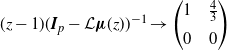 $(z-1)({\boldsymbol{I}}_{p} - \mathcal{L}\boldsymbol{\mu}(z))^{-1} \to \begin{pmatrix} 1\;\;\;\;\; & \frac{4}{3} \\[5pt] 0\;\;\;\;\; & 0 \end{pmatrix}$
as
 $z \to 1$
. The martingale
 $W_t(1)$
corresponding to the parameter
 $\alpha = 1$
is given by
 \begin{align*} W_t(1) = \sum_{u \in \mathcal{C}_t} \mathrm{e}^{-S(u)} {e}_{\tau(u)} \begin{pmatrix} 1\;\;\;\;\; & \frac{4}{3} \\[5pt] 0\;\;\;\;\; & 0 \end{pmatrix} = \sum_{\substack{u \in \mathcal{C}_t:\\[2pt] {e}_{\tau(u)} = 1}} \mathrm{e}^{-S(u)} \begin{pmatrix} 1\;\;\;\;\; & \frac{4}{3} \end{pmatrix} \end{align*}
and
 $W_0(1) = {1}_{\{\tau(\varnothing) = 1\}} \begin{pmatrix} 1\;\;\;\;\; & \frac{4}{3} \end{pmatrix}$
. In particular, when the branching process starts with an individual of type 2, the martingale
 $W_t(1) = (0\ 0)$
for all
 $t \geq 0$
.
4. Proofs of the main results
Proof of Theorem
2.2. First, we consider
 $\mathcal{Z}^{\phi_{\lambda}}_t$
for
 $t \geq 0$
. We write
 \begin{align*} \mathcal{Z}^{\phi_{\lambda}}_t & = \sum_{u\in\mathcal{I}}({\boldsymbol{I}}_{{k}_\lambda} \otimes {e}_{\tau(u)})\phi_{\lambda,u}(t-S(u)) \\[5pt] & = \sum_{u\in\mathcal{I}}{1}_{\{S(u)\leq t\}}\biggl(\int_{(t-S(u),\infty)}\exp\!(\lambda,t-S(u)-s) \otimes \boldsymbol{\xi}_u^{\tau(u)}(\mathrm{d}\mathit{s})\biggl)\vec{{\boldsymbol{A}}}_\lambda. \end{align*}
Notice that by Assumptions 2.1 and 2.2, for any
 $t \geq 0$
, with probability 1, we have
 $S(u)\gt t$
for all but finitely many
 $u \in \mathcal{I}$
. Hence, the sum above is almost surely a finite sum of integrable random variables and thus finite almost surely, showing that
 $\mathcal{Z}^{\phi_{\lambda}}_t$
and hence also
 $W_t(\lambda)$
is well defined. Using
 $\exp\!(\lambda,-t)=\exp\!(\lambda,-t)\otimes 1$
, we obtain
 \begin{align} W_t(\lambda) = \exp\!(\lambda,-t)\mathcal{Z}^{\phi_{\lambda}}_t & = \sum_{u\in\mathcal{I}}{1}_{\{S(u)\leq t\}}\biggl(\int_{(t-S(u),\infty)}\exp\!(\lambda,-S(u)-s) \otimes \boldsymbol{\xi}_u^{\tau(u)}(\mathrm{d}\mathit{s})\biggl)\vec{{\boldsymbol{A}}}_\lambda \notag \\[5pt] & = \sum_{u\in\mathcal{I}}\sum_{j=1}^{N_u}{1}_{\{S(u)\leq t\lt S(uj)\}}(\!\exp\!(\lambda,-S(uj)) \otimes {e}_{\tau(uj)}) \vec{{\boldsymbol{A}}}_\lambda . \end{align}
Substituting
 ${1}_{\{S(u)\leq t\lt S(uj)\}}={1}_{\mathcal{C}_t}(uj)$
in (4.1) gives (2.10). We further deduce that
 \begin{align*} W_t(\lambda) & = \sum_{u\in\mathcal{I}}\sum_{j=1}^{N_u}{1}_{\{S(u)\leq t\lt S(uj)\}}(\!\exp\!(\lambda,-S(uj)) \otimes {e}_{\tau(uj)}) \vec{{\boldsymbol{A}}}_\lambda \\[5pt] & = \sum_{u\in\mathcal{I}}\sum_{j=1}^{N_u}({1}_{\{S(u)\leq t\}}-{1}_{\{S(uj)\leq t\}})(\!\exp\!(\lambda,-S(uj)) \otimes {e}_{\tau(uj)})\vec{{\boldsymbol{A}}}_\lambda \\[5pt] & = \sum_{u\in\mathcal{I}}{1}_{\{S(u)\leq t\}}(\!\exp\!(\lambda,-S(u))\otimes 1)\biggl(\sum_{j=1}^{N_u} \exp\!(\lambda,-X_{u,j}) \otimes {e}_{\tau(uj)}\biggl)\vec{{\boldsymbol{A}}}_\lambda \\[5pt] & \quad - \sum_{|u|\geq 1}{1}_{\{S(u)\leq t\}}(\!\exp\!(\lambda,-S(u)) \otimes {e}_{\tau(u)})\vec{{\boldsymbol{A}}}_\lambda. \end{align*}
Note that the decomposition of the sum is justified, since both sums almost surely contain only finitely many nonzero terms. We proceed by writing
 \begin{align} W_t(\lambda) & = \sum_{u\in\mathcal{I}}{1}_{\{S(u)\leq t\}}(\!\exp\!(\lambda,-S(u)) \otimes 1)\Biggl(\sum_{j=1}^{N_u} \exp\!(\lambda,-X_{u,j}) \otimes {e}_{\tau(uj)}\Biggl)\vec{{\boldsymbol{A}}}_\lambda \notag \\[5pt] & \quad - \sum_{|u|\geq 1}{1}_{\{S(u)\leq t\}}(\!\exp\!(\lambda,-S(u)) \otimes {e}_{\tau(u)}) \vec{{\boldsymbol{A}}}_\lambda \notag \\[5pt] & = {1}_{[0,\infty)}(t)({\boldsymbol{I}}_{{k}_\lambda} \otimes {e}_{\tau(\varnothing)})\vec{{\boldsymbol{A}}}_\lambda + \sum_{u\in\mathcal{I}}{1}_{\{S(u)\leq t\}}(\!\exp\!(\lambda,-S(u)) \otimes {e}_{\tau(u)})Y_u. \end{align}
At this point, it can be readily seen that
 $W_t(\lambda)$
is
 $\mathcal{F}_t$
-measurable. Indeed, this follows from the fact that each summand in the preceding expression is
 $\mathcal{F}_t$
-measurable, which, in turn, can be verified directly from the definition of
 $\mathcal{F}_t$
and basic measurability arguments. The next item on the agenda is the proof of the integrability of
 $W_t(\lambda)$
. We estimate as follows, using the matrix operator norm
 $\|\cdot\|$
:
 \begin{align*} \mathbb{E}\Bigg[\Bigg\|\sum_{u\in\mathcal{I}}{1}_{\{S(u)\leq t\}}(\!\exp\!(\lambda,-S(u)) \otimes {e}_{\tau(u)}) Y_u\Bigg\|\Bigg] & \leq \sum_{u\in\mathcal{I}}\mathbb{E}\big[{1}_{\{S(u)\leq t\}}\|\exp\!(\lambda,-S(u)) \otimes {e}_{\tau(u)}\|\| Y_u\|\big] \\[5pt] & \leq C\mathbb{E}\Bigg[\sum_{u\in\mathcal{I}}{1}_{\{S(u)\leq t\}}\Bigg] \end{align*}
for some finite constant
 $C\gt0$
. It is well known in the theory of multi-type branching processes (see, e.g., [Reference Kolesko, Meiners and Tomic11, Proposition 2.1]) that under Assumptions 2.1 and 2.2 the expected number of births up to and including time t is finite for every
 $t \geq 0$
.
The final property to be verified is the martingale property. To this end, let us fix
 $0 \leq s \lt t$
. Then
 $W_t(\lambda) - W_s(\lambda) = \sum_{u\in\mathcal{I}}{1}_{\{s\lt S(u)\leq t\}}(\!\exp\!(\lambda,-S(u))\otimes{e}_{\tau(u)})Y_u$
. Here, it suffices to show that
 $\mathbb{E}\big[{1}_{\{s\lt S(u)\leq t\}}(\!\exp\!(\lambda,-S(u))\otimes{e}_{\tau(u)})Y_u \mid \mathcal{F}_s\big]=0$
a.s. To prove this, we first claim that, for any
 $v \in \mathcal{I}$
and
 $A\in \mathcal{A}_v$
,
 $\mathbb{E}\big[{1}_{A\cap\{S(v)\leq s \}}{1}_{\{s\lt S(u)\leq t\}}(\!\exp\!(\lambda,-S(u),k)\otimes{e}_{\tau(u)})Y_u\big]=0$
. Indeed, if
 $u \preceq v$
, then
 $S(u) \leq S(v)$
, and thus
 ${1}_{\{S(v) \leq s\}}{1}_{\{s \lt S(u) \leq t\}} = 0$
. On the other hand, if
 $u \not\preceq v$
, then
 $\sigma(\mathcal{A}_v \cap \mathcal{A}_{u|_{|u|-1}})$
is independent of
 $\boldsymbol{\xi}_u$
, and in particular of
 $Y_u$
. Consequently, the expectation again vanishes, since
 $\mathbb{E}[Y_u] = 0$
. The argument carries over if we take a finite intersection of sets of the form
 $A_u \cap \{S(u)\leq s\}$
for
 $A_u\in\mathcal{A}_u$
and different
 $u\in\mathcal{I}$
. Dynkin’s
 $\pi$
–
 $\lambda$
theorem then implies the martingale property. In particular, (2.9) holds.
Proof of Theorem
2.3. Throughout the proof, we write
 $\theta := \operatorname{Re}(\lambda)$
. We first show that Assumption 2.3 implies
 $\mathbb{E}[\|Y\|^q]\lt\infty$
. Using the submultiplicative property of matrix norms, we obtain, with
 $\|\cdot\|_{\mathrm{HS}}$
denoting the Hilbert–Schmidt norm,
 \begin{align*} \mathbb{E}\big[\lVert Y\rVert^q_{\mathrm{HS}}\big] & = \mathbb{E}\biggl[\biggl\lVert\biggl(\int\exp\!(\lambda,-s) \otimes \boldsymbol{\xi}(\mathrm{d}\mathit{s}) - ({\boldsymbol{I}}_{{k}_\lambda}\!\otimes{\boldsymbol{I}}_{p})\biggl)\vec{{\boldsymbol{A}}}_{\lambda}\biggl \rVert^q_{\mathrm{HS}}\biggl] \\[5pt] & \leq \lVert\vec{{\boldsymbol{A}}}_{\lambda}\rVert^q_{\mathrm{HS}}\mathbb{E}\biggl[\biggl\lVert\biggl( \int\exp\!(\lambda,-s) \otimes \boldsymbol{\xi}(\mathrm{d}\mathit{s}) - ({\boldsymbol{I}}_{{k}_\lambda}\!\otimes{\boldsymbol{I}}_{p})\biggl)\biggl\rVert^q_{\mathrm{HS}}\biggl]. \end{align*}
Since, for any
 $p\times p$
matrix
 ${\boldsymbol{A}}$
,
 $\lVert{\boldsymbol{A}}-{\boldsymbol{I}}_{p}\rVert^q_{\mathrm{HS}} \leq (\lVert{\boldsymbol{A}} \rVert_{\mathrm{HS}} + \lVert{\boldsymbol{I}}_{p}\rVert_{\mathrm{HS}})^q \leq c_q(\lVert{\boldsymbol{A}} \rVert^q_{\mathrm{HS}}+1)$
for some finite constant
 $c_q\gt0$
, we conclude that
 \begin{align*} \mathbb{E}[\lVert Y\rVert^q_{\mathrm{HS}}] & \leq c_q\lVert\vec{{\boldsymbol{A}}}_{\lambda}\rVert^q_{\mathrm{HS}}\mathbb{E}\biggl[\biggl\lVert\biggl( \int\exp\!(\lambda,-s) \otimes \boldsymbol{\xi}(\mathrm{d}\mathit{s}) - ({\boldsymbol{I}}_{{k}_\lambda}\!\otimes{\boldsymbol{I}}_{p})\biggl)\biggl\rVert^q_{\mathrm{HS}}\biggl] \\[5pt] & \leq c_q\lVert\vec{{\boldsymbol{A}}}_{\lambda}\rVert^q_{\mathrm{HS}}\biggl(1 + \mathbb{E}\biggl[\biggl\lVert\biggl(\int\exp\!(\lambda,-s) \otimes \boldsymbol{\xi}(\mathrm{d}\mathit{s})\biggl)\biggl \rVert^q_{\mathrm{HS}}\biggl]\biggl) \\[5pt] & \leq Cc_q\lVert\vec{{\boldsymbol{A}}}_{\lambda}\rVert^q_{\mathrm{HS}}\Biggl(1 + \sum_{l=0}^{{k}_\lambda -1}\sum_{i,j=1}^p\mathbb{E}\biggl[\biggl(\int\mathrm{e}^{-\operatorname{Re}(\lambda)s}s^{l}\, \xi^{i,j}(\mathrm{d}\mathit{s})\biggl)^q\biggl]\Biggl) \end{align*}
for some constant
 $C \gt 0$
, where in the final step we used the fact that the function
 $x \mapsto x^{q/2}$
is subadditive on
 $[0, \infty)$
. The finiteness of the last expression follows from Assumption 2.3.
We now turn to the
 $L^q$
-boundedness, i.e.
 $\sup_{t \geq 0} \mathbb{E}[\|W_t(\lambda)\|^q] \lt \infty$
, which, in view of (4.2), is equivalent to
 \begin{align} \mathop{\sup}\nolimits_{t \geq 0}\mathbb{E}\Bigg[\Bigg\|\sum_{u\in\mathcal{I}}{1}_{\{S(u)\leq t\}} (\!\exp\!(\lambda,-S(u)) \otimes {e}_{\tau(u)})Y_u\Bigg\|^q\Bigg] \lt \infty. \end{align}
Let
 $x\in\mathbb{R}^{1\times k}$
and
 $y\in \mathbb{R}^{p\times 1}$
be fixed vectors. Then
 $(x\otimes 1)$
and
 $(1\otimes y)$
are vectors in the space
 $\mathbb{R}^{1\times k}\otimes\mathbb{R}$
and
 $\mathbb{R}\otimes \mathbb{R}^{p\times 1}$
, respectively. We assume that
 $|x|, |y| \leq 1$
, where
 $|\cdot|$
denotes the Euclidean norm, here and throughout. For (4.3) to hold, it is sufficient to show that
 \begin{align*} & (x \otimes 1)\!\sum_{u\in\mathcal{I}}{\!1}_{\{S(u)\leq t\}}(\!\exp\!(\lambda,-S(u)) \otimes {e}_{\tau(u)})Y_u(1\otimes y) = \sum_{u\in\mathcal{I}}{\!1}_{\{S(u)\leq t\}}(x\exp\!(\lambda,-S(u)) \otimes {e}_{\tau(u)})Y_u y \end{align*}
is an
 $L^q$
-bounded martingale. Define
 $M_n(\lambda) := \sum_{|u|\leq n}{1}_{\{S(u)\leq t\}}(x\exp\!(\lambda,-S(u)) \otimes {e}_{\tau(u)})Y_u y$
and notice that its nth increment, namely
 \begin{align*} M_n(\lambda) - M_{n-1}(\lambda) = \sum_{|u|=n}{1}_{\{S(u)\leq t\}}(x\exp\!(\lambda,-S(u)) \otimes {e}_{\tau(u)})Y_u y, \end{align*}
is, conditionally on
 $\sigma(\tau(\varnothing), \boldsymbol{\xi}_u \colon |u| \lt n)$
, a weighted sum of independent, centered random variables for
 $n \in \mathbb{N}_0$
. Therefore, we may apply the von Bahr–Esseen inequality (see [Reference von Bahr and Esseen16, Theorem 2] for the original version and [Reference Iksanov, Kolesko and Meiners6, Lemma A.1] for a version for complex-valued random variables) twice: once directly, and once conditionally on
 $\sigma(\tau(\varnothing), \boldsymbol{\xi}_u \colon |u| \lt n)$
, to obtain
 \begin{align*} & \mathbb{E}\Biggl[\Biggl|\sum_{u\in\mathcal{I}}{1}_{\{S(u)\leq t\}}(x\exp\!(\lambda,-S(u))\otimes{e}_{\tau(u)}) Y_u y\Biggl|^q\Biggl] \\ & \qquad \leq 4\sum_{n=0}^\infty\mathbb{E}\Biggl[\Biggl|\sum_{|u|=n}{1}_{\{S(u)\leq t\}} (x\exp\!(\lambda,-S(u))\otimes{e}_{\tau(u)})Y_u y\Biggl|^q\Biggl] \\ & \qquad \leq 4\sum_{n=0}^\infty\mathbb{E}\Bigg[\mathbb{E}\Biggl[\Biggl|\sum_{|u|=n}{1}_{\{S(u)\leq t\}} (x\exp\!(\lambda,-S(u))\otimes{e}_{\tau(u)})Y_u y\Biggl|^q \mid \tau(\varnothing), \boldsymbol{\xi}_u \colon |u| \lt n \Biggl]\Bigg] \\ & \qquad \leq 16\mathbb{E}\Biggl[\sum_{u\in\mathcal{I}}{1}_{\{S(u)\leq t\}} |(x\exp\!(\lambda,-S(u))\otimes{e}_{\tau(u)})Y_u y|^q\Biggl]. \end{align*}
Then, using
 $|x|,|y|\leq 1$
and the independence of
 ${1}_{\{S(u)\leq t\}}(\!\exp\!(\lambda,-S(u),k_\lambda)\otimes{e}_{\tau(u)})$
and
 $Y_u$
,
 \begin{align*} \sum_{u\in\mathcal{I}}\mathbb{E}[|{1}_{\{S(u)\leq t\}}(x\exp\!(\lambda,-S(u))\otimes{e}_{\tau(u)})Y_u y|^q] \leq \sum_{n=0}^\infty\sum_{|u|=n}\mathbb{E}\bigl[\lVert\exp\!(\lambda,-S(u))\rVert^q\bigl]\mathbb{E}[\lVert Y_u\rVert^q]. \end{align*}
Using
 $\mathbb{E}[\|Y\|^q] \leq \mathbb{E}[\|Y\|_{\mathrm{HS}}^q]\lt\infty$
and the condition
 $\theta \gt \alpha/q$
, we find
 $\delta \gt 0$
so small that
 $q(\theta - \delta)\gt\alpha$
and some finite constant
 $C_\delta\gt0$
such that
 \begin{align*} \sum_{n=0}^\infty\sum_{|u|=n}\mathbb{E}\bigl[\lVert\exp\!(\lambda,-S(u))\rVert^q\bigl] \mathbb{E}[\lVert Y_u\rVert^q] & \leq C_\delta\mathbb{E}[\|Y\|^q]\sum_{n=0}^\infty\mathbb{E}\Biggl[ \sum_{|u|=n}\mathrm{e}^{-q(\theta-\delta)S(u)}\Biggl] \\ & \leq C_\delta\mathbb{E}[\|Y\|^q]\mathbb{E}[{e}_{\tau(\varnothing)}]\sum_{n=0}^\infty \mathcal{L}\boldsymbol{\mu}(q(\theta-\delta))^n\mathbf{1}^\top \\ & \leq C_\delta\mathbb{E}[\|Y\|^q]\mathbb{E}[{e}_{\tau(\varnothing)}] ({\boldsymbol{I}}_{p}-\mathcal{L}\boldsymbol{\mu}(q(\theta-\delta)))^{-1}\mathbf{1}^\top \lt \infty, \end{align*}
where
 $\mathbf{1}\in\mathbb{R}^{1\times p}$
denotes the row vector with all entries equal to one. Further, notice that we have used that
 $q(\theta - \delta)\gt\alpha$
, hence the spectral radius of
 $\mathcal{L}\boldsymbol{\mu}(q(\theta-\delta))$
is strictly smaller than 1 and the infinite series of matrices converges. The proof is complete.
Appendix A. The Kronecker product
Consider an
 $m\times n$
matrix
 $A = (a_{ij})_{i=1,\ldots,m,j=1,\ldots,n}$
and a
 $k\times l$
matrix B. Following [Reference Graham4, Chapter 2.2], the Kronecker product of the matrices A and B, denoted by
 $A \otimes B$
, is defined as the
 $mk\times nl$
matrix
 \begin{align*} A\otimes B := \begin{pmatrix} a_{11}B\;\;\;\;\; & \cdots\;\;\;\;\; & a_{1n}B \\[5pt] \vdots\;\;\;\;\; & \ddots\;\;\;\;\; & \vdots \\[5pt] a_{m1}B\;\;\;\;\; & \cdots\;\;\;\;\; & a_{mn}B \end{pmatrix}\!.\end{align*}
In other words, the Kronecker product increases the dimensions of both matrices by replacing each entry of A with a scaled copy of the entire matrix B, resulting in a block matrix.
Appendix B. Exponential matrices
For
 $\lambda \in {\kern0pt\mathcal{D}(\mathcal{L}\boldsymbol{\mu})}^{\mathrm{o}}$
satisfying (2.1), we use a multiplicative family of matrices
 $\exp\!(\lambda,x)$
,
 $x\in \mathbb{R}$
, similar to that used in [Reference Iksanov, Kolesko and Meiners7, (4.10)], namely, we define the upper triangular
 ${k}_\lambda \times {k}_\lambda$
matrix
 \begin{align*} \exp\!(\lambda, x) = (\!\exp_{ij}(\lambda, x))_{i,j=1,\ldots,{k}_\lambda} := \mathrm{e}^{\lambda x} \begin{pmatrix} 1\;\;\;\;\; & x\;\;\;\;\; & \dfrac{x^2}{2!}\;\;\;\;\; & \cdots\;\;\;\;\; & \dfrac{x^{{k}_\lambda-1}}{({k}_\lambda-1)!} \\[12pt] 0\;\;\;\;\; & 1\;\;\;\;\; & x\;\;\;\;\; & \cdots\;\;\;\;\; & \dfrac{x^{{k}_\lambda-2}}{({k}_\lambda-2)!} \\[5pt] 0\;\;\;\;\; & 0\;\;\;\;\; & 1\;\;\;\;\; & \cdots\;\;\;\;\; & \vdots \\[5pt] \vdots\;\;\;\;\; & \vdots\;\;\;\;\; & \vdots\;\;\;\;\; & \ddots\;\;\;\;\; & x \\[5pt] 0\;\;\;\;\; & \cdots\;\;\;\;\; & \cdots\;\;\;\;\; & 0\;\;\;\;\; & 1 \end{pmatrix}\!.\end{align*}
We have
 \begin{align} \exp\!(\lambda, x)\exp\!(\lambda,y) = \exp\!(\lambda,x+y), \quad x,y \in \mathbb{R}.\end{align}
Writing
 $J_\lambda$
for the
 ${k}_\lambda \times {k}_\lambda$
Jordan matrix
 \begin{align*} J_{\lambda} = \begin{pmatrix} \lambda\;\;\;\;\; & 1\;\;\;\;\; & 0\;\;\;\;\; & \cdots\;\;\;\;\; & 0 \\[5pt] 0\;\;\;\;\; & \lambda\;\;\;\;\; & 1\;\;\;\;\; & \cdots\;\;\;\;\; & 0 \\[5pt] \vdots\;\;\;\;\; & \vdots\;\;\;\;\; & \ddots\;\;\;\;\; & \cdots\;\;\;\;\; & \vdots \\[5pt] 0\;\;\;\;\; & \cdots\;\;\;\;\; & \cdots\;\;\;\;\; & \lambda\;\;\;\;\; & 1 \\[5pt] 0\;\;\;\;\; & \cdots\;\;\;\;\; & \cdots\;\;\;\;\; & \cdots\;\;\;\;\; & \lambda \\[5pt] \end{pmatrix}\!,\end{align*}
we infer (B.1) from
 $\exp\!(\lambda,x) = \exp\!(x\, J_\lambda)$
from the functional equation of the matrix exponential function.
Acknowledgements
Part of this work was conducted during visits of Matthias Meiners and Ivana Tomic to the University of Wrocł aw, for which they express their gratitude for the warm hospitality.
Funding information
Matthias Meiners and Ivana Tomic were supported by DFG grant ME3625/4-1.
Competing interests
There were no competing interests to declare which arose during the preparation or publication process of this article.


 Open access

