2 Mathematical set-up

We consider an adiabatic, inviscid, three-dimensional, horizontally and vertically unbounded, continuously stratified, rapidly rotating fluid. For simplicity, we assume that the background rotation is uniform so that the Coriolis frequency $f$ is constant. We also assume that the buoyancy frequency $N$ , defined by $N^{2}=g\unicode[STIX]{x1D70C}_{0}^{-1}\text{d}\unicode[STIX]{x1D70C}/\text{d}z$ under the Boussinesq approximation, is constant so that the stratification is linear with depth. Here $g$ is the gravitational acceleration, $\unicode[STIX]{x1D70C}_{0}$ is the mean density and $\unicode[STIX]{x1D70C}(z)$ is the basic state density. The Boussinesq approximation assumes that the density variations are small compared to the mean density. This assumption is valid for the oceans. For convenience, we rescale the physical vertical coordinate by the ratio $N/f$ . Typically, $N/f\gg 1$ in most parts of the oceans (see Dijkstra Reference Dijkstra2008). In this vertically stretched reference frame, the equations become independent of $N$ and $f$ , hence our results are valid for all values of $N/f$ . We define the Froude number $Fr=U/(NH)$ , where $U$ is a characteristic scale of horizontal velocity and $H$ is a characteristic vertical length scale, and the Rossby number $Ro=U/(fL)$ , where $L$ is a characteristic horizontal length scale. For rapid background rotation $Ro\ll 1$ and strong stratification $Fr^{2}\ll Ro$ , the Boussinesq equations can be asymptotically expanded in terms of small $Ro$ and $Fr$ to obtain the QG model (see Vallis Reference Vallis2006 for details). The equations read

(2.1) $$\begin{eqnarray}q={\displaystyle \frac{\unicode[STIX]{x2202}^{2}\unicode[STIX]{x1D713}}{\unicode[STIX]{x2202}x^{2}}}+{\displaystyle \frac{\unicode[STIX]{x2202}^{2}\unicode[STIX]{x1D713}}{\unicode[STIX]{x2202}y^{2}}}+{\displaystyle \frac{\unicode[STIX]{x2202}^{2}\unicode[STIX]{x1D713}}{\unicode[STIX]{x2202}z^{2}}},\end{eqnarray}$$

with

(2.2) $$\begin{eqnarray}{\displaystyle \frac{\text{D}q}{\text{D}t}}={\displaystyle \frac{\unicode[STIX]{x2202}q}{\unicode[STIX]{x2202}t}}-{\displaystyle \frac{\unicode[STIX]{x2202}\unicode[STIX]{x1D713}}{\unicode[STIX]{x2202}y}}{\displaystyle \frac{\unicode[STIX]{x2202}q}{\unicode[STIX]{x2202}x}}+{\displaystyle \frac{\unicode[STIX]{x2202}\unicode[STIX]{x1D713}}{\unicode[STIX]{x2202}x}}{\displaystyle \frac{\unicode[STIX]{x2202}q}{\unicode[STIX]{x2202}y}}=0,\end{eqnarray}$$

where $q$ defined by (2.1) is the QG potential vorticity (PV) anomaly, hereinafter referred to as PV for simplicity, $\unicode[STIX]{x1D713}$ is the streamfunction and $\text{D}/\text{D}t$ stands for the material derivative. Equation (2.2) states that PV is materially conserved for an adiabatic, inviscid fluid. It should be noted that the full dynamics is controlled by the PV, $q$ , a single scalar quantity. Equation (2.1) can formally be inverted using the Green’s function for the three-dimensional Laplacian

(2.3) $$\begin{eqnarray}G(\boldsymbol{x};\boldsymbol{x}^{\prime })=-{\displaystyle \frac{1}{4\unicode[STIX]{x03C0}|\boldsymbol{x}-\boldsymbol{x}^{\prime }|}},\end{eqnarray}$$

which by construction provides the streamfunction, evaluated at $\boldsymbol{x}=(x,y,z)$ , induced by a point vortex of unit intensity located at $\boldsymbol{x}^{\prime }=(x^{\prime },y^{\prime },z^{\prime })$ . Differentiating explicitly the Green’s function with respect to $x$ and $y$ , respectively, gives the velocity $v=\unicode[STIX]{x2202}\unicode[STIX]{x1D713}/\unicode[STIX]{x2202}x$ and $u=-\unicode[STIX]{x2202}\unicode[STIX]{x1D713}/\unicode[STIX]{x2202}y$ induced by the point vortex. Second-order derivatives provide the velocity gradients which are used to study the linear stability of the point vortex arrays; see appendix A for details. For finite core vortices, the inversion of (2.1) leads to volume integrals. The fluid domain is represented by horizontal layers of equal thickness $\unicode[STIX]{x0394}z$ in which the Green’s function (and its derivatives) can be integrated analytically. The remaining (horizontal) surface integrals are converted to contour integrals over the contours bounding the horizontal cross-sections of the uniform PV vortices using Green’s theorem.

The numerical method used to perform the simulation of the evolution of the flow is the purely Lagrangian contour surgery algorithm introduced by Dritschel (Reference Dritschel1988) for two-dimensional flows and adapted to three-dimensional QG flows by Dritschel & Saravanan (Reference Dritschel and Saravanan1994) and Dritschel (Reference Dritschel2002). Contour surgery is an extension of contour dynamics (see Zabusky, Hughes & Roberts Reference Zabusky, Hughes and Roberts1979), which allows one to control the complexity of the vortex bounding contours by topological reconnections.

To obtain finite-volume vortex equilibria, we use an iterative method which makes the vortex bounding contours converge to streamlines. The approach is based on a method developed by Pierrehumbert (Reference Pierrehumbert1980) for two-dimensional flows and adapted to three-dimensional QG flows by Reinaud & Dritschel (Reference Reinaud and Dritschel2002) and further used in Reinaud & Dritschel (Reference Reinaud and Dritschel2009) and Reinaud & Carton (Reference Reinaud and Carton2015). The method is presented in appendix B. The linear stability of the finite-volume vortex arrays is addressed by analysing deformation modes of the vortex bounding contours (Reinaud & Dritschel Reference Reinaud and Dritschel2002) and is briefly described in appendix C. It includes a mode representing the displacement of the full contours, hence the relative displacement of the vortices.

3 Point vortices

We first consider arrays of point vortices. We refer to the vortices lying along the ring as the peripheral vortices. Vortex $i$ carries an intensity or ‘charge’ of potential vorticity $\unicode[STIX]{x1D6E4}_{i}$ , which has the physical dimension of a volume-integrated PV (see e.g. Gryanik Reference Gryanik1983). The $m$ peripheral vortices are identified by their index $1\leqslant i\leqslant m$ . If an additional central vortex is present, it is identified by the index $0$ . For convenience, we define the strength of vortex $i$ by $\unicode[STIX]{x1D705}_{i}=\unicode[STIX]{x1D6E4}_{i}/(4\unicode[STIX]{x03C0})$ . The point vortex problem has a unique length scale and a unique time scale, which can both be chosen arbitrarily. The length scale is set by the radius $R=1$ of the ring on which the $m$ peripheral vortices are located, and the time scale is implicitly defined by taking $\unicode[STIX]{x1D705}_{i}=\unicode[STIX]{x1D705}=1$ for $1\leqslant i\leqslant m$ , where $\unicode[STIX]{x1D705}$ is the common strength of the peripheral vortices. Without loss of generality, the ring of vortices is located on the horizontal plane $z=0$ . The location of the $m$ peripheral vortices at $t=0$ is $(x_{i},y_{i},z_{i})=(\cos \unicode[STIX]{x1D703}_{i},\sin \unicode[STIX]{x1D703}_{i},0)$ , where $\unicode[STIX]{x1D703}_{i}=2\unicode[STIX]{x03C0}(i-1)/m$ . The central vortex has strength $\unicode[STIX]{x1D705}_{0}$ and is located at $(0,0,d)$ . We take $d\geqslant 0$ without loss of generality. We define $\unicode[STIX]{x1D6FC}=\unicode[STIX]{x1D705}_{0}/\unicode[STIX]{x1D705}$ . 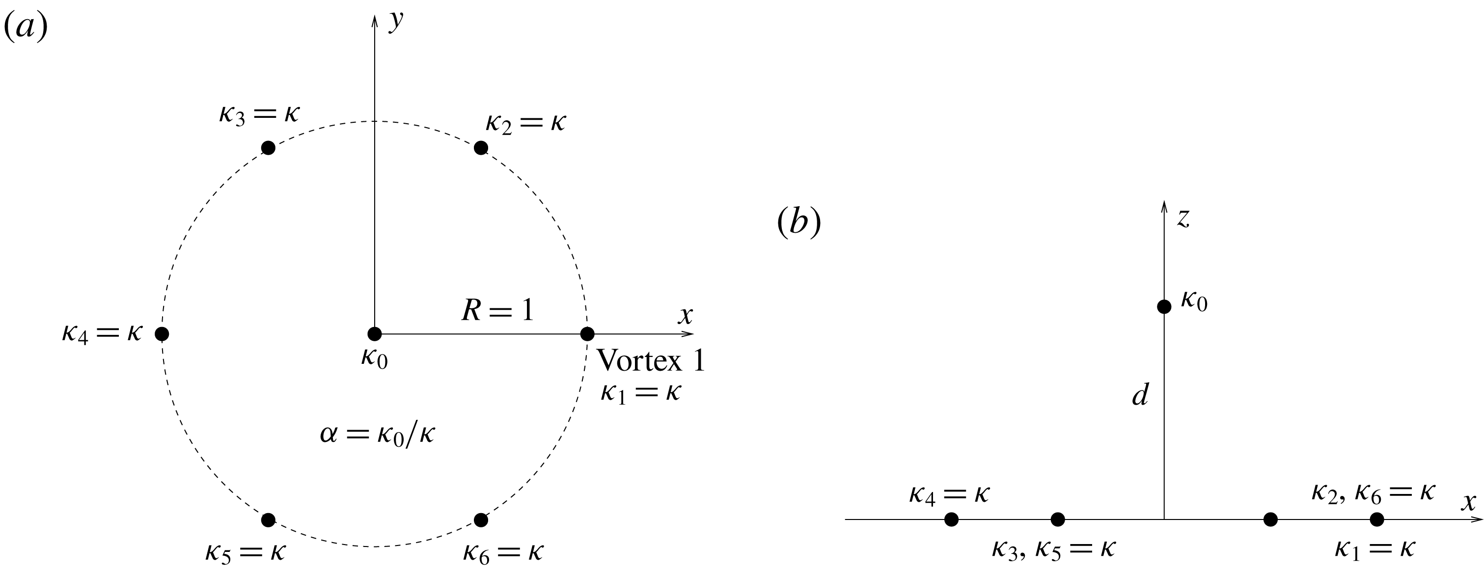The general geometry of the vortex array is shown in figure 1.

Figure 1.

Geometry of the point vortex array and definition of the parameters presented for $6+1$ vortices: (a) view from the top in the $x,y$ -plane, (b) side view in the $x,z$ -plane.

We analyse the linear stability of the $m$ -vortex arrays and of the ( $m+1$ )-vortex arrays for $d=0$ and $\unicode[STIX]{x1D6FC}=\pm 1$ for $2\leqslant m\leqslant 8$ . When $d=0$ , all $m+1$ vortices are coplanar. We analyse the normal modes of perturbation of the horizontal locations of the vortices $(x_{i}^{\prime },y_{i}^{\prime },0)$ . We do not consider perturbations of the vertical location of the vortices, which could also modify the distance separating the vortices, as no external QG flow may move the point vortices in the vertical direction. We do not consider perturbations on the strength of the vortices either. These modes of perturbations have a time dependence proportional to $\text{e}^{\unicode[STIX]{x1D70E}t}=\text{e}^{\unicode[STIX]{x1D70E}_{r}t}(\cos \unicode[STIX]{x1D70E}_{i}t+\text{i}\sin \unicode[STIX]{x1D70E}_{i}t)$ , where the real part of $\unicode[STIX]{x1D70E}$ is the growth rate of the mode, $\unicode[STIX]{x1D70E}_{r}$ , and its imaginary part, $\unicode[STIX]{x1D70E}_{i}$ , is its frequency. There are $n_{m}=2m$ modes for the $m$ -vortex problem or $n_{m}=2m+2$ modes for the ( $m+1$ )-vortex problem. This approach is the same as the one used in different contexts in Reinaud & Carton (Reference Reinaud and Carton2015, Reference Reinaud and Carton2016) and is further described in appendix A.

Figure 2.

(a) Maximum growth rate $\unicode[STIX]{x1D70E}^{max}$ versus the number of vortices $m$ for QG point vortices in a three-dimensional, continuously stratified fluid. The results for the $m$ -vortex problem are indicated by black $+$ , and the ( $m+1$ )-vortex problem with $d=0$ and $\unicode[STIX]{x1D6FC}=1$ by blue ♢, while $\unicode[STIX]{x1D6FC}=-1$ by red ○. (b) The same as (a) but for two-dimensional vortices for comparison.

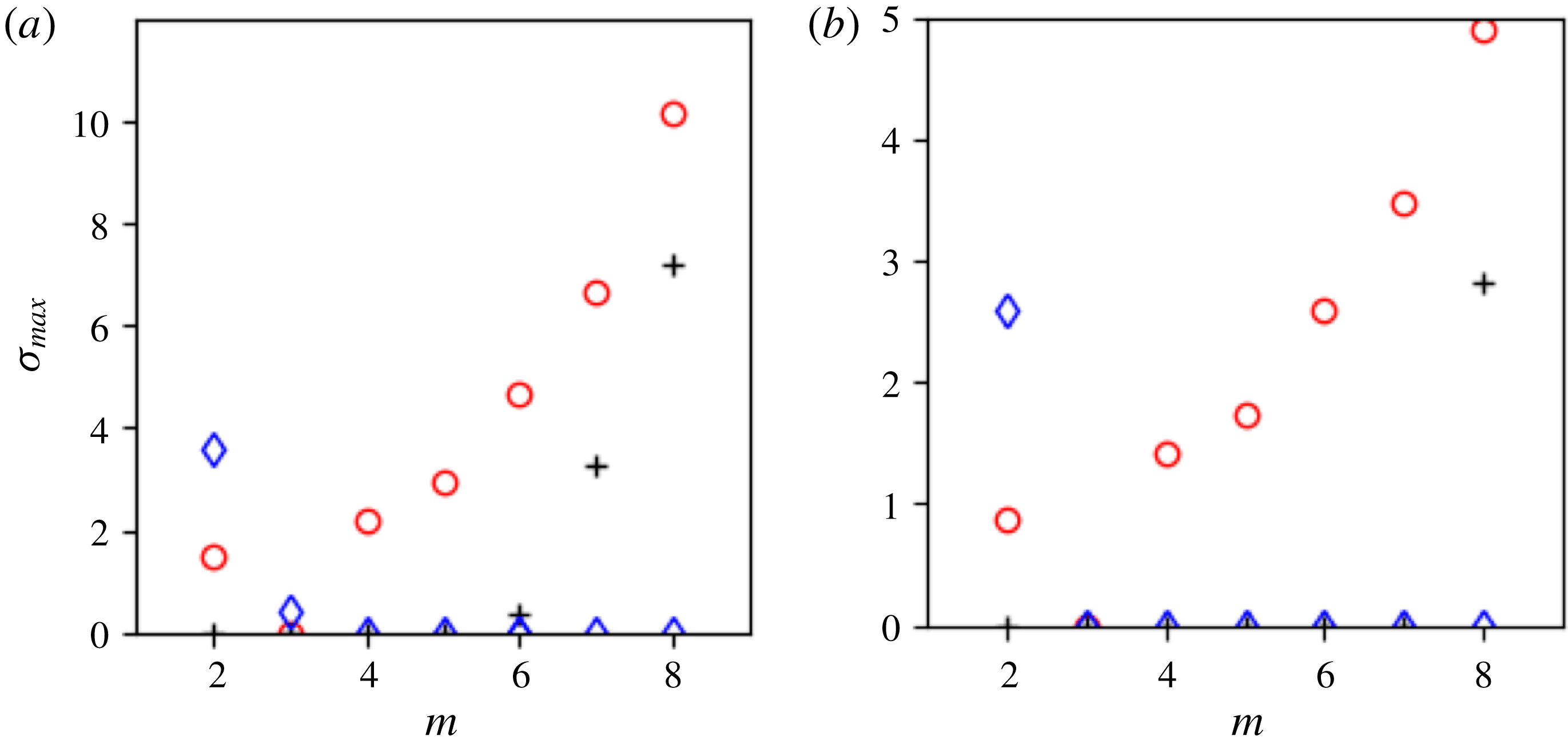
Figure 2 shows the maximum growth rate $\unicode[STIX]{x1D70E}^{max}=\max _{1\leqslant j\leqslant n_{m}}\{{\unicode[STIX]{x1D70E}_{r}}_{j}\}$ versus the number of peripheral vortices $m$ . For comparison, similar results for two-dimensional vortices are included. The results presented here are obtained using the same numerical technique as for the QG computations but adapted to the two-dimensional situation. For the two-dimensional vortices, the circulation of the peripheral vortices is set to $\unicode[STIX]{x1D6E4}_{2D}=2\unicode[STIX]{x03C0}$ . When a central vortex is added, $d=0$ by construction, and again we use a central vortex of circulation $\unicode[STIX]{x1D6E4}_{0}=\pm \unicode[STIX]{x1D6E4}_{2D}=\pm 2\unicode[STIX]{x03C0}$ . The parameter $\unicode[STIX]{x1D6FC}$ is also used to denote the circulation ratio of the central vortex to the peripheral ones.

For the $m$ -vortex problem, results shown in figure 2 indicate that the three-dimensional QG vortex array is ‘less linearly stable’ than the equivalent two-dimensional one. Indeed, the two-dimensional vortex arrays are linearly stable for $m\leqslant 7$ (see figure 2 b, Thomson (Reference Thomson1883) and Kurakin & Yudovich (Reference Kurakin and Yudovich2002)), whereas the three-dimensional QG vortex arrays are only linearly stable for $m\leqslant 5$ (see figure 2 a). Recall that the difference between the two situations lies in the nature of the Green’s function, which is $G_{2D}(\boldsymbol{x}^{\prime };\boldsymbol{x}^{\prime })=(1/2\unicode[STIX]{x03C0})\ln |\boldsymbol{x}-\boldsymbol{x}^{\prime }|$ for the two-dimensional case in contrast with (2.3). Hence the velocity gradients are proportional to $r^{-3}$ in QG, where $r=|\boldsymbol{x}-\boldsymbol{x}^{\prime }|$ is the distance between the source and the evaluation point, compared to $r^{-2}$ for the two-dimensional vortices.

Figure 3.

Trajectories of the point vortices for the unstable ( $2+1$ )-vortex problem for (a)  $\unicode[STIX]{x1D6FE}=-1$ , (b)  $\unicode[STIX]{x1D6FE}=0$ and (c)  $\unicode[STIX]{x1D6FE}=1$ .

We also observe a strong influence of the presence of a central vortex. For $d=0$ , $\unicode[STIX]{x1D6FC}=1$ and $m>3$ , the presence of the like-signed central vortex stabilises the array. The vortex array indeed remains linearly stable for $m=6$ up to $8$ . The vortex array with $m=9$ is linearly unstable. Similar stabilising effects of a central, like-signed vortex were first observed for two-dimensional geostrophic vortices by Morikawa & Swenson (Reference Morikawa and Swenson1971). It should be noted that the like-signed central vortex has, however, a destabilising effect for a small number of peripheral vortices $m=2,3$ . On the other hand, the presence of a coplanar opposite-signed central vortex with $\unicode[STIX]{x1D6FC}=-1$ destabilises the ring, except for the special case $m=3$ . Overall, these trends are also observed for the two-dimensional case, as shown in figure 2(b).

We next show the nonlinear evolution of a selection of point vortex arrays. Figure 3 shows the trajectories of the point vortices for ( $2+1$ )-vortex arrays with $\unicode[STIX]{x1D6FC}=-1$ , $0$ and $1$ . All trajectories are shown in the reference frame steadily rotating with the equilibrium. In this reference frame, the departure of the vortices from their initial position is the result of instability. In the case where $\unicode[STIX]{x1D6FC}=-1$ , shown in figure 3(a), the central vortex and each peripheral vortex have equal and opposite strengths. The central and one of the peripheral vortices get closer together to form a vortex dipole, which moves away from the origin. This vortex dipole has an overall zero strength as the strengths of the vortices compensate. To conserve the angular impulse $J=2\unicode[STIX]{x03C0}\sum _{i=0}^{2}\unicode[STIX]{x1D705}_{i}(x_{i}^{2}+y_{i}^{2})=2\unicode[STIX]{x03C0}\unicode[STIX]{x1D705}R^{2}$ , the other peripheral vortex orbits around the origin. For $\unicode[STIX]{x1D6FC}=0$ , the central vortex has zero strength and thus is a passive particle. The remaining two vortices are stable (see figure 2 a). The evolution of the vortex array is shown in figure 3(b). The two peripheral vortices, shown in red and black, remain indeed at their initial locations. The passive particle, however, moves away from its initial location, which is a hyperbolic critical point. It should be noted that instabilities have also been found in shallow water for such degenerate tripoles, in which the central pole is passive, by Kizner (Reference Kizner2014) – see in particular their figure 5. This is further detailed below when we address the influence of the parameter  $\unicode[STIX]{x1D6FC}$ .

For $\unicode[STIX]{x1D6FC}=1$ , the vortex array is unstable. The evolution of the vortices is shown in figure 3(c). Here all three vortices have equal strength. The trajectories indicate that one of the peripheral vortices may move towards the origin while the central vortex moves outwards to conserve both linear and angular impulses. Similar behaviours where the central vortex moves towards the ring while one of the peripheral vortices moves towards the centre have been observed for larger values of $m$ as shown below.

Figure 4.

Trajectories of the point vortices for the unstable ( $3+1$ )-vortex problem for $\unicode[STIX]{x1D6FE}=1$ .

Results presented in figure 2(a) also indicate that the ( $3+1$ )-vortex array with $\unicode[STIX]{x1D6FC}=1$ is unstable. The evolution of the vortices is shown in figure 4. The trajectories of the vortices appear to be chaotic. We also see that all vortices transitorily pass near the origin. For a larger number of vortices ( $m>4$ ) and $\unicode[STIX]{x1D6FC}=1$ , the results (not shown) also indicate that the unstable equilibria lead to a chaotic motion of the vortices.

Figure 5.

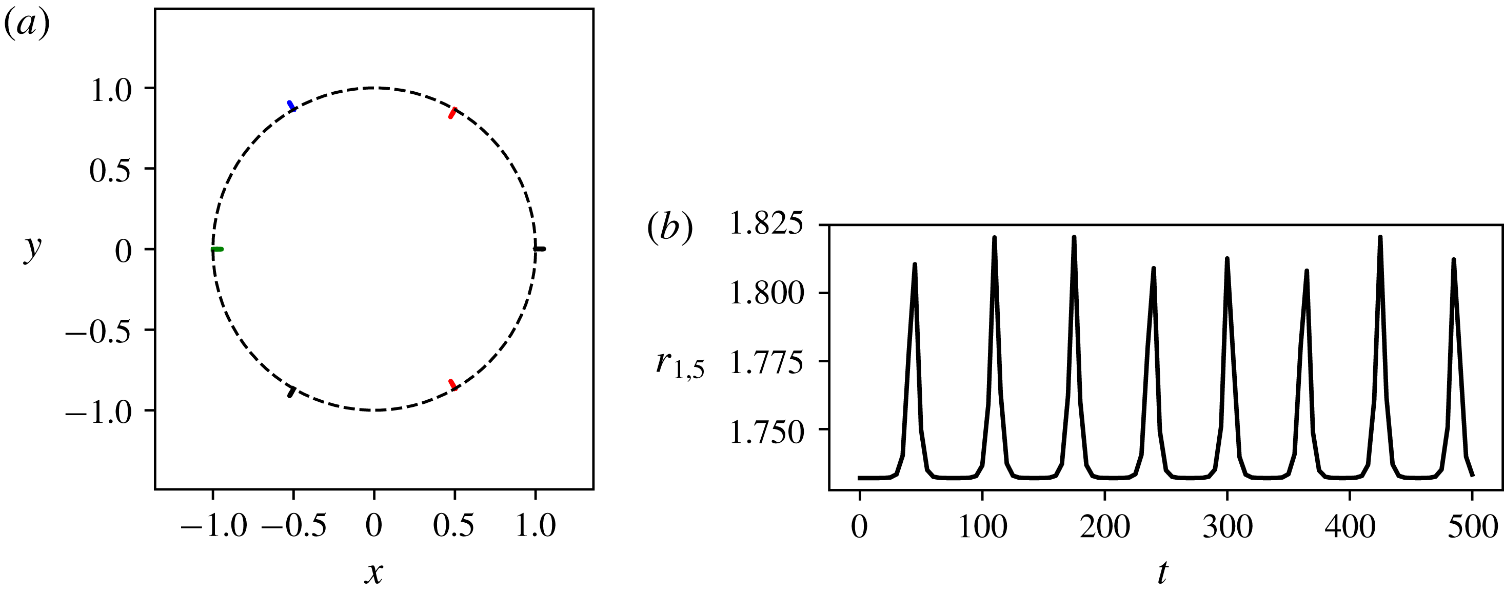
(a) Trajectories of the point vortices for the unstable six-vortex problem for $0\leqslant t\leqslant 500$ . The unfilled circle indicates the initial position of the vortices. The dashed circle indicates the ring of radius $R=1$ where the vortices initially lie. (b) Distance $r_{1,5}=|\boldsymbol{x}_{1}-\boldsymbol{x}_{5}|$ between the vortex 1 and vortex 5 versus time.

Figure 6.

(a) Trajectories of the point vortices for the unstable seven-vortex problem for $0\leqslant t\leqslant 10$ . The unfilled circle indicates the initial position of the vortices.

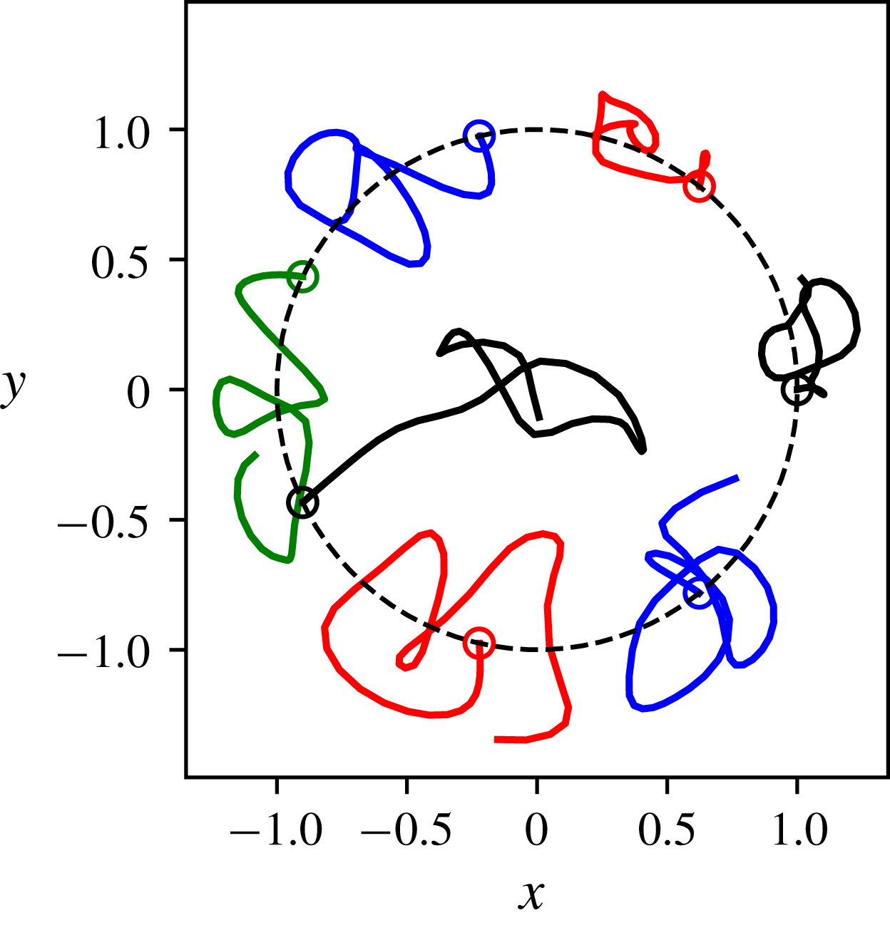
The evolution of the weakly unstable six-vortex array is shown in figure 5. The weak instability results in a very small oscillatory motion of the vortices. The oscillation is due to nonlinear effects. The oscillation is better seen by plotting the evolution of the distance $r_{1,5}=|\boldsymbol{x}_{1}-\boldsymbol{x}_{5}|$ between vortex 1 and vortex 5, initially located at $(1,0,0)$ and $(-1/2,-\sqrt{3}/2)$ , respectively. After an exponential growth of the distance $r_{1,5}$ from its initial value, nonlinear effects bring the vortices back to their initial positions. This relative motion repeats quasi-periodically. The evolution of the unstable seven-vortex array is shown in figure 6. In this case the instability is much stronger and the point vortices have an apparent chaotic motion. It can be noted that one of the seven peripheral vortices moves (temporarily) near the centre of the array, indicating that the stable ( $6+1$ )-vortex array acts as an attractor.

By symmetry, the ( $m+1$ )-vortex array remains in steady rotation even if $d\neq 0$ and $|\unicode[STIX]{x1D6FC}|\neq 1$ , provided the central vortex is located on the vertical axis passing through the centre of the ring, which is the rotation axis of the system. Moreover, in this case the system remains in steady rotation for all values of $\unicode[STIX]{x1D6FC}$ . The central vortex strength $\unicode[STIX]{x1D705}_{0}$ and its vertical location $d$ modify the angular velocity of the equilibrium but do not break the equilibrium. They also affect its stability properties. We thus examine the stability properties of the ( $m+1$ )-vortex array in the parameter space $(\unicode[STIX]{x1D6FC},d)$ distinguishing the cases $\unicode[STIX]{x1D6FC}<0$ and $\unicode[STIX]{x1D6FC}>0$ for clarity.

Figure 7.

Contours of maximum growth rates of instability for the ( $2+1$ )-vortex problem in a three-dimensional, continuously stratified fluid in the place $(|\unicode[STIX]{x1D6FC}|,d)$ for (a)  $\unicode[STIX]{x1D6FC}<0$ and (b)  $\unicode[STIX]{x1D6FC}>0$ .

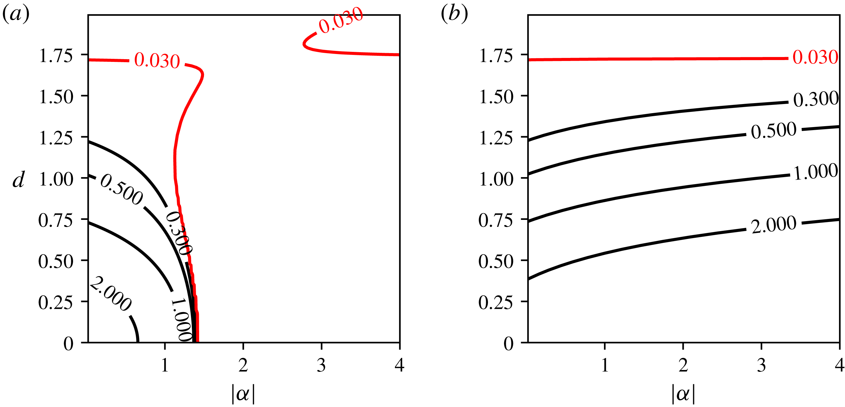
We first present results for $m=2$ in figure 7. The vortex array is unstable for small $d$ and $\unicode[STIX]{x1D6FC}>0$ . The growth rate of the instability decays as $d$ is increased as a consequence of the decrease of the interaction between the central vortex and the peripheral vortices as seen in figure 7(b). The same is true for $-1.5<\unicode[STIX]{x1D6FC}<0$ (see figure 7 a). A stronger opposite-sign central vortex is, however, able to stabilise the vortex array. We recover in particular that the ( $2+1$ )-vortex array with $\unicode[STIX]{x1D6FC}=-2$ is linearly stable as established analytically by Reinaud & Carton (Reference Reinaud and Carton2015). Results also indicate that the ( $2+1$ )-vortex array is unstable for $\unicode[STIX]{x1D6FC}\rightarrow 0$ , i.e. for a vanishing strength central vortex. In the complete absence of a central vortex, a pair of like-sign point vortices, a two-body system, is stable. The instability observed for the ( $2+1$ )-vortex, a three-body system, with $\unicode[STIX]{x1D6FC}\rightarrow 0$ is due to the fact that the central vortex lies initially at a hyperbolic critical point (a stagnation point separating two trajectories around the peripheral vortices). Hence, although the locations of the peripheral vortices are stable, the vanishing central vortex is unstable. This explains the trajectory of the central vortex observed in figure 3(b). Similar results are discussed by Kizner (Reference Kizner2014) for QG two-layer and single-layer flows, where the pair of active vortices is shown to be stable but an instability can be observed due to the possible motion of the passive central vortex.

Figure 8.

Contours of maximum growth rates of instability for $m$ identical vortices on a ring with an opposite-signed central vortex ( $\unicode[STIX]{x1D6FC}<0$ ), for QG point vortices in a three-dimensional, continuously stratified fluid in the plane $(|\unicode[STIX]{x1D6FC}|,d)$ with $m=3$ (a),  $4$ (b),  $5$ (c) and  $6$ (d).

Figure 9.

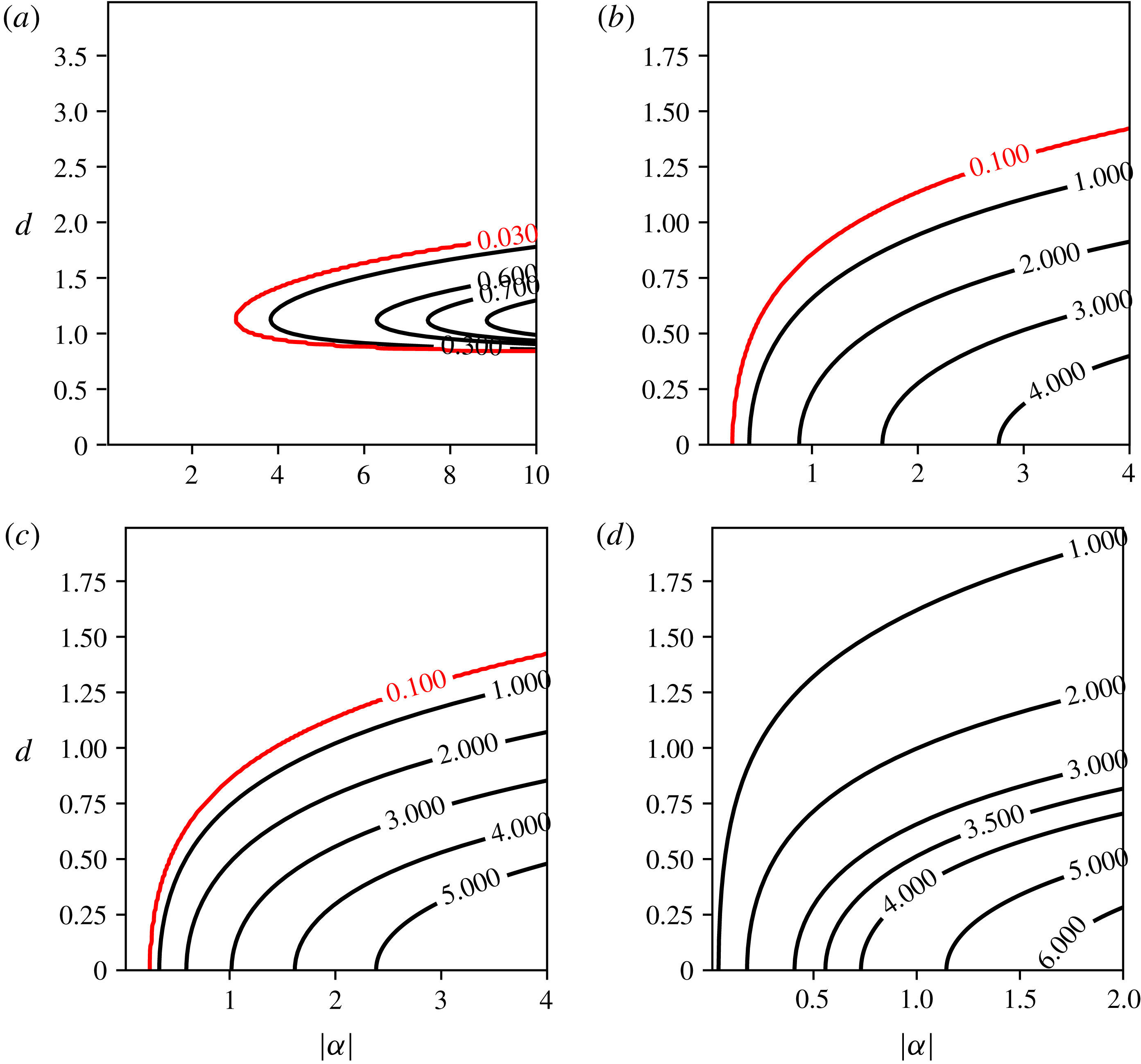
Contours of maximum growth rates for $n$ identical vortices on a ring with a like-signed central vortex for QG point vortices in a three-dimensional, continuously stratified fluid in the place $(|\unicode[STIX]{x1D6FC}|,d)$ for $m=3$ (a),  $4$ (b),  $5$ (c) and  $6$ (d). The panel for $m=6$ offers a close-up for small $d$ . Results for $m=6$ and larger $d$ are shown in figure 10.

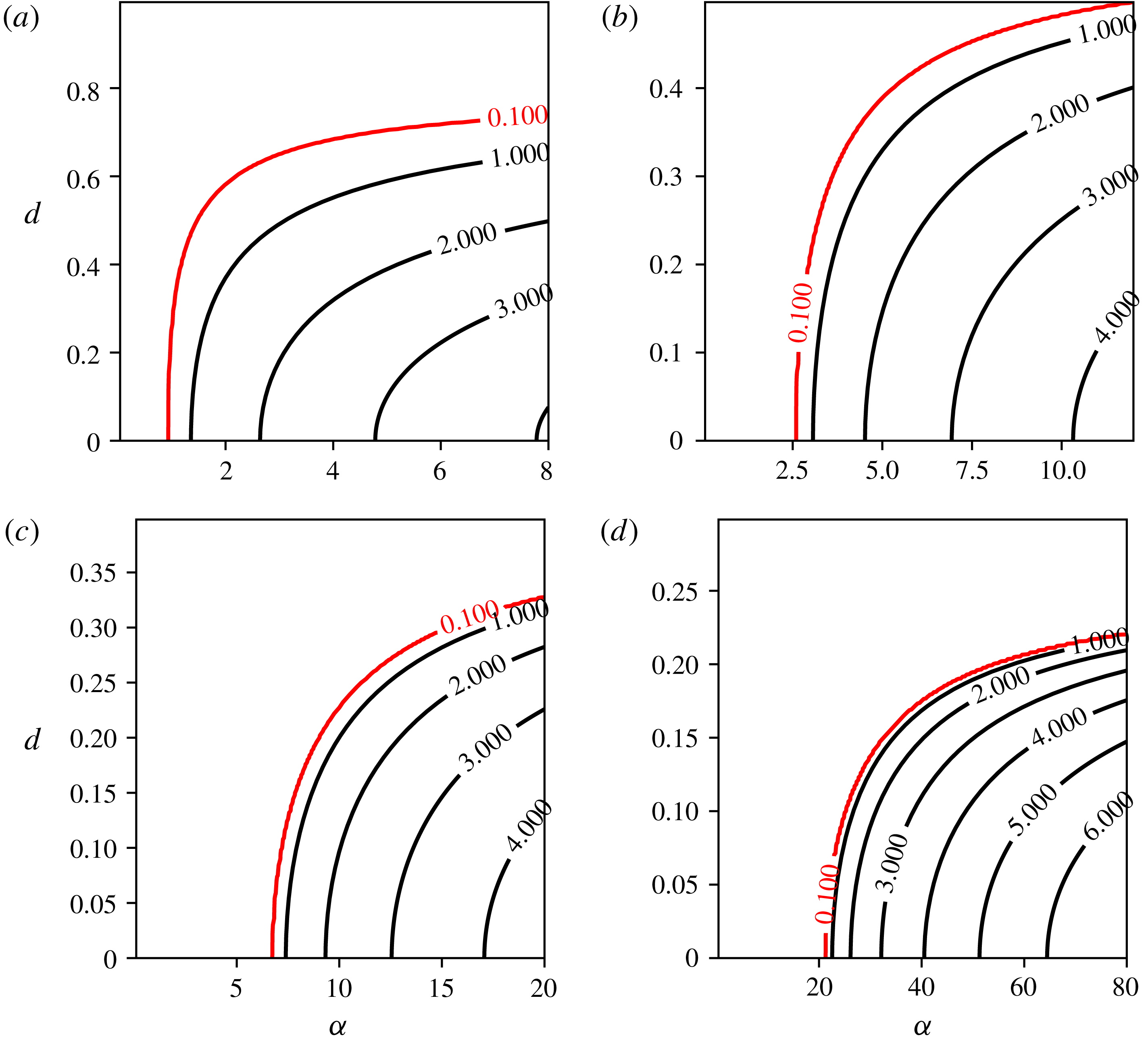
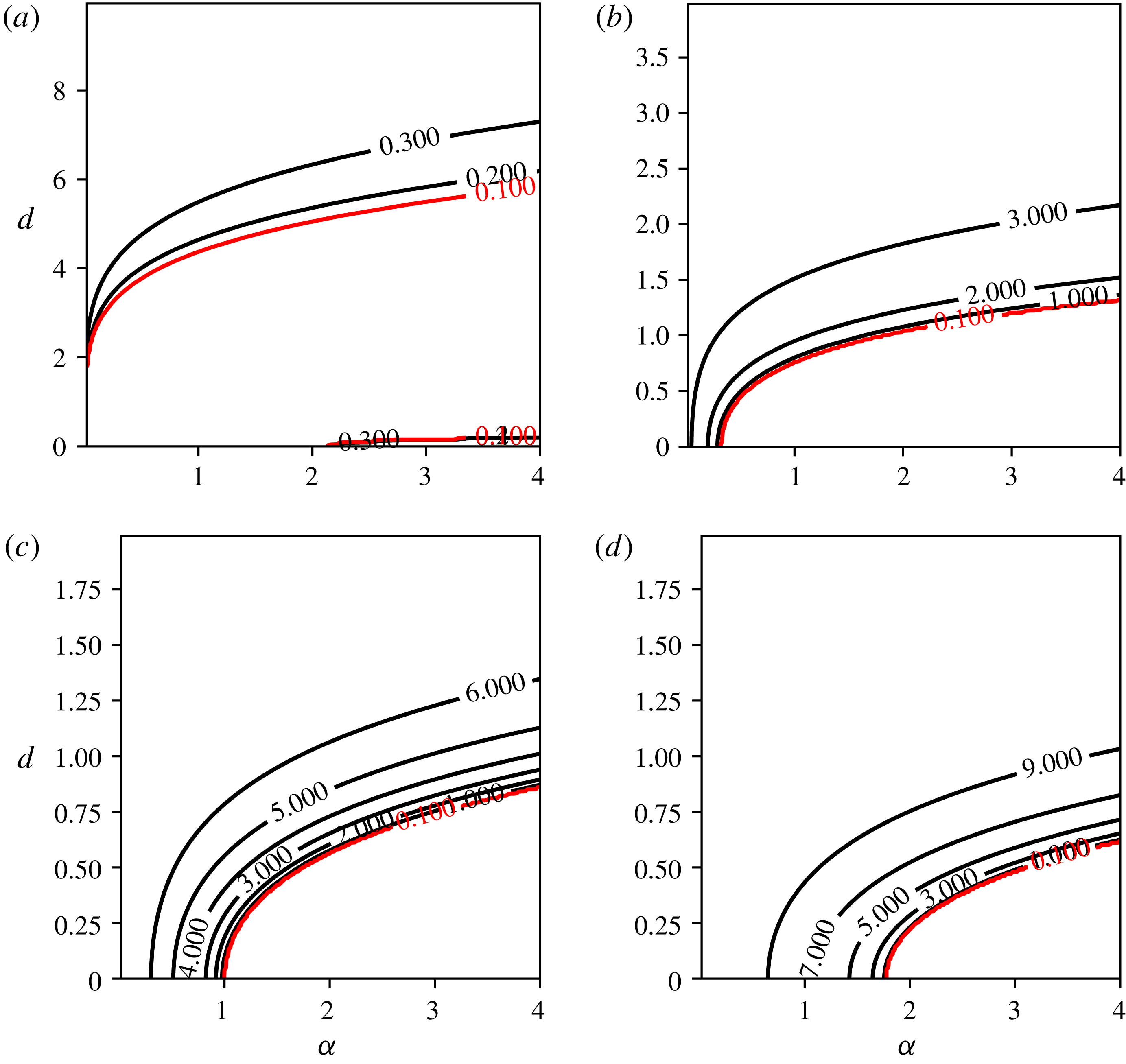
Next, results are presented in figure 8 for $\unicode[STIX]{x1D6FC}<0$ and in figure 9 for $\unicode[STIX]{x1D6FC}>0$ and $3\leqslant m\leqslant 6$ . First, the results show that linearly unstable modes can be found for all values of $m$ investigated, in particular if $|\unicode[STIX]{x1D6FC}|$ is larger than a threshold which depends on $m$ . Since the influence of the central vortex on the peripheral vortices decreases with its height $d$ , this growth rate of the instability is larger for small $d$ . This is true for all cases but for $m=3$ and $\unicode[STIX]{x1D6FC}<0$ , as seen in figure 8. We also confirm that an opposite-signed central vortex favours instability as the threshold in $|\unicode[STIX]{x1D6FC}|$ which separates the linearly stable and linearly unstable regions is lower, for a given $d$ , when $\unicode[STIX]{x1D6FC}<0$ . Finally, we see that, for $\unicode[STIX]{x1D6FC}<0$ , increasing $m$ makes the vortex array more unstable. On the other hand, for $\unicode[STIX]{x1D6FC}>0$ , we see that increasing $m$ first shifts the threshold in $\unicode[STIX]{x1D6FC}$ to larger values. For $m=6$ there is in fact a second, weaker, unstable mode which arises from $(\unicode[STIX]{x1D6FC},d)=(0,0)$ and persists for $\unicode[STIX]{x1D6FC}>0$ and $d\neq 0$ (see figure 10 a). Recall indeed that the array of six point vortices is unstable. Therefore, one expects for $m\geqslant 6$ that, when $\unicode[STIX]{x1D6FC}\rightarrow 0$ , the ( $m+1$ )-vortex problem will be linearly unstable as well. This mode becomes the dominant mode for $m\geqslant 7$ (see figure 10). The particular case $m=6$ is interesting, as in that case we see that a weak central vortex located in the plane of the ring is able to stabilise the vortex array, while instability is recovered if the weak central vortex is vertically offset by a value of $d$ of the order of the ring radius $R=1$ .

Figure 10.

Contours of maximum growth rates for $n$ identical vortices on a ring with a like-signed central vortex for QG point vortices in a three-dimensional, continuously stratified fluid in the place $(|\unicode[STIX]{x1D6FC}|,d)$ for $m=6$ (a),  $7$ (b),  $8$ (c) and  $9$ (d).

4 Finite-volume vortices

We next turn our attention to finite-volume vortices of uniform potential vorticity. The objective of this part is to provide the generic shapes and characteristics of finite core equilibria for $2\leqslant m\leqslant 7$ at the highest possible resolution. We again investigate vortex arrays with and without a central vortex. We do not intend to provide at this stage a complete catalogue of the equilibria throughout a large parameter space, which arguably would be of little interest. There is an additional length scale in the problem, associated with the size of the vortices. In this problem, the radius of the ring along which the peripheral vortices lie is no longer fixed but is varied. Recall that this distance sets the distance between the vortices. We are still free to fix a length scale in the problem. Without loss of generality we set the height of the vortices to 1, in the reference frame vertically stretched by $N/f$ . We restrict attention to vortices having a unit mean height-to-width aspect ratio, $h_{v}/r_{v}$ , measured in the stretched reference frame due to the numerical cost of the computations. Here, $h_{v}$ is the half-height of the vortices and $r_{v}$ is their mean horizontal radius. Such vortices therefore have a unit Burger number $Bu=(h_{v}/r_{v})^{2}=1$ . The vortices are, however, pancake-like in physical space. The specific choice of vortices with unit height-to-width aspect ratio is, however, consistent with findings in QG turbulence where it has been shown that vortices have typically a near-unity aspect ratio (close to 0.8) (see Reinaud, Dritschel & Koudella Reference Reinaud, Dritschel and Koudella2003). It should be noted that this specific choice imposes a limitation on the variety of equilibria we investigate.

The branches of equilibria stem from vortex arrays of infinitely distant spherical vortices in the vertically stretched reference frame. The vortices volume is $V=4\unicode[STIX]{x03C0}h_{v}r_{v}^{2}/3=\unicode[STIX]{x03C0}/6$ , and their PV is set to $q=4\unicode[STIX]{x03C0}$ . This means that the time scale associated with the vortices, inversely proportional to $q$ , and their strength $qV$ are the same in all experiments. The $m$ vortices are each discretised in the vertical direction by $n_{c}=83$ horizontal layers. The vortex bounding contours are discretised by $n_{p}=4n_{c}$ nodes. It should be noted that the numerical cost of the algorithms grows as $m^{2}n_{p}^{2}n_{c}^{2}$ . We focus on equilibria having imposed symmetries.

First, all $m$ vortices have the same shape. Vortex $i$ , $2\leqslant i\leqslant m$ , is the image of vortex 1 by a rotation of angle $2(i-1)\unicode[STIX]{x03C0}/m$ . Second, each vortex is symmetric with respect to a vertical plane passing through the vortex centre and the vertical axis of rotation (the $z$ -axis). Similar numerical set-ups and symmetries are imposed for the ( $m+1$ )-vortex problem. We focus on cases where the central vortex lies in the plane containing the ring of peripheral vortices $(d=0)$ . We consider the two cases where the PV of the central vortex is $q_{0}=\pm 4\unicode[STIX]{x03C0}$ . In these cases, the central vortex has an imposed $m$ -fold symmetry, and the number of nodes $n_{p}$ discretising each contour is adjusted to be divisible by $m$ . Even when reducing the computational load by taking advantage of the problem symmetries, determining a single equilibrium state at these resolutions for $7+1=8$ vortices can take up to a day on a single core of a modern processor. This imposes limitations on the number of states one can determine.

For each configuration, and a given value of $m$ , we determine the family of equilibrium states spanned by the ratio of distance $\unicode[STIX]{x1D6FF}$ separating the peripheral vortices and the centre of the domain, which is the centre of rotation, to the mean vortex radius $r_{v}=0.5$ . Branches of solutions are sought until we reach an end point of the solution branch, namely when the vortices touch. The choice of the distance to be used depends on the configuration, as not all distances between a point defined on the vortices and the rotation centre vary monotonically along the solution branches, due to the deformation of the vortices. In practice, the distance $\unicode[STIX]{x1D6FF}$ is the distance between the innermost edge of the vortices and the centre of the ring when the peripheral vortices develop a sharp inner edge. On the other hand, $\unicode[STIX]{x1D6FF}$ is the distance between the outermost edge and the centre of the ring when the vortices develop a flat or slightly convex inner surface. We start the branches of solution from large separation distances. When an equilibrium is reached by the iterative method, the distance is reduced and the numerical method is resumed for the new separation. It should be noted that, if the radius of the ring tends to infinity, spherical vortices should be in mutual equilibrium. The shape of the vortices departs from a sphere as the vortices are located closer together. The equilibrium vortices are deformed to be able to steadily withstand the shear (proportional to $r^{-3}$ ) they induce on each other. The numerical method used to determine the equilibrium states is iterative and is described in appendix B.

We determine the equilibria for the $m$ -vortex problem for $2\leqslant m\leqslant 7$ . It should be noted that the equilibria for $m=2$ were originally obtained at lower resolution by Reinaud & Dritschel (Reference Reinaud and Dritschel2002) and at high resolution in Reinaud & Dritschel (Reference Reinaud and Dritschel2018).

Figure 11.

Top view of the vortex bounding contours to the $m$ -vortex equilibria at the end of the solution branch where the vortices touch. The grey scale indicates the height of the contour: lighter grey contours are nearer the top.

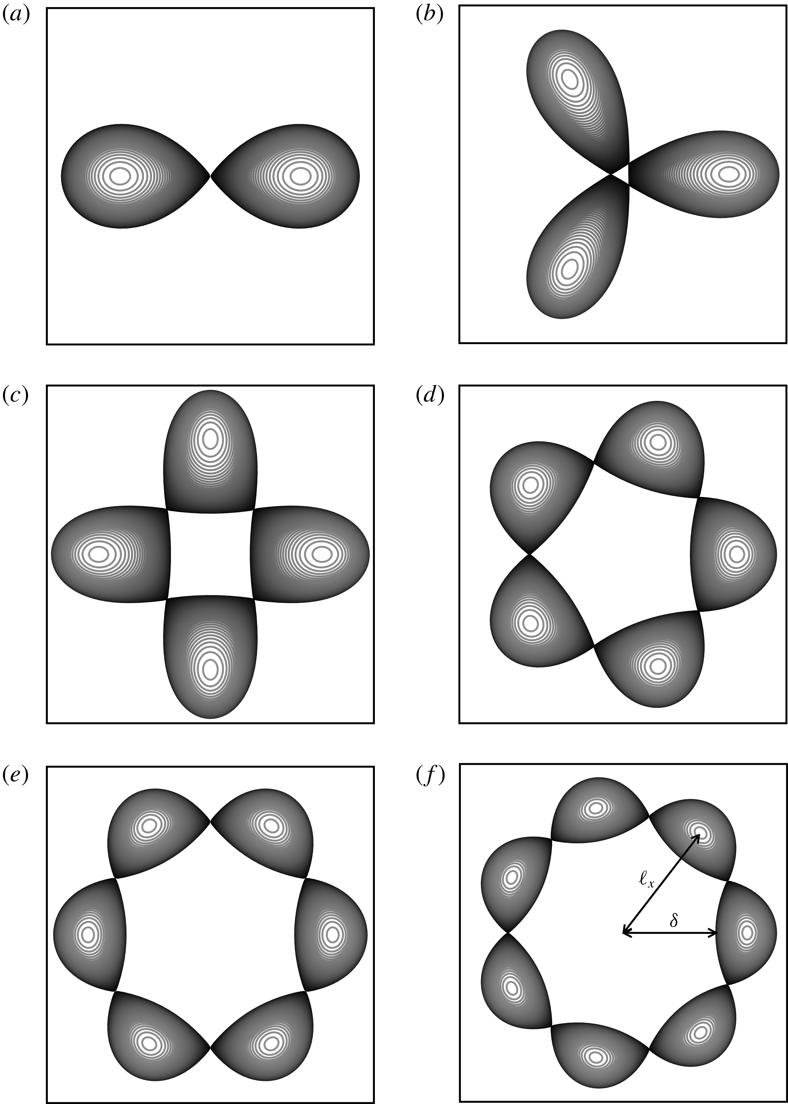
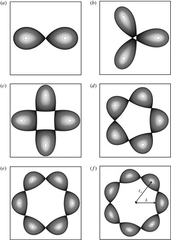
We first describe the shape of the equilibria obtained numerically and we address next their linear stability. The method used for the linear stability analysis is described in appendix C. Figure 11 shows a top view of the vortex bounding contours at the end of the solution branch, where the vortices nearly touch for $m=2$ to $m=7$ . Except for $m=2$ , the vortices near the end point of the branch do not exhibit a single sharp inner edge. This is in contrast with the two-dimensional equilibria shown by Dritschel (Reference Dritschel1985) (in particular their figure 2) where a single sharp inner edge forms for $m\leqslant 4$ . Instead, for $m\geqslant 3$ the innermost part of the vortices flattens and remains slightly convex. Vortices touch by their side at the end point of the solution branch.

Figure 12.

Maximum growth rate $\unicode[STIX]{x1D70E}^{max}$ of instability versus the inner gap $\unicode[STIX]{x1D6FF}$ for the finite-volume $m$ -vortex problem for $m=3$ (solid black), $4$ (dotted black), $5$  (dashed-dotted black), $6$ (solid red) and $7$ (dotted red).

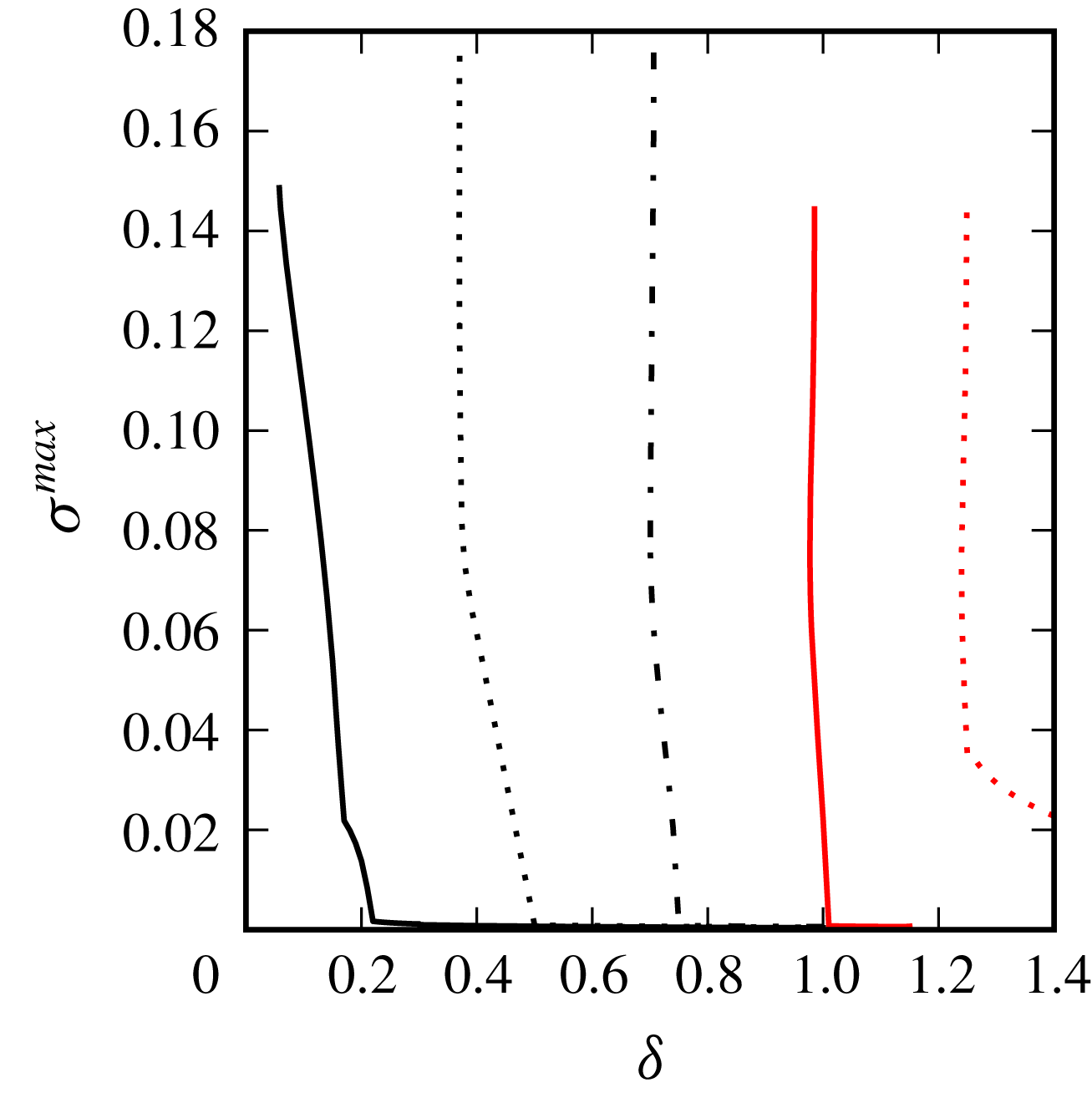
Figure 12 shows the maximum growth rate $\unicode[STIX]{x1D70E}^{max}=\max \{\unicode[STIX]{x1D70E}_{r}\}$ versus the distance $\unicode[STIX]{x1D6FF}$ between the innermost edge of the vortices and the centre of rotation. Results show that the equilibria are unstable for $\unicode[STIX]{x1D6FF}$ less than a threshold depending on $m$ . Importantly, unstable equilibria are found for all $m$ for all three configurations. Finite-volume vortices can deform and therefore can be sensitive to deformation modes as well as displacement modes. By construction, only the displacement modes can be captured by the analysis of the stability of systems of point vortices. Moreover, there is a fundamental difference between deformation modes which affect the shape of the vortices and displacement modes which move the vortices. If a point vortex equilibrium is sensitive to a displacement mode, the point vortex equilibrium is fundamentally unstable, i.e. it is unstable for all separation distances between the vortices. The distance influences the magnitude of the growth rate, but does not change the nature of the stability properties. On the other hand, the deformation modes for finite-volume vortices can be triggered when the vortices are close enough to each other, as seen in figure 12. In practice such deformation modes are associated with the phase locking of vorticity Rossby waves travelling on the vortex boundaries – see Dritschel (Reference Dritschel1995) for a discussion for two-dimensional vortices. A mode with non-zero growth rate is observed for $m=7$ for all distances and is associated with the displacement mode. The growth rate of the instability increases as the vortices are closer together. This is related to the increase of the strain vortices induced on each other. It should be noted, however, that the similar (but much weaker) displacement instability mode for $m=6$ observed in the point vortex calculation is not clearly noticeable for the finite-volume vortex equilibria. We conjecture that the deformed finite-volume vortices have adapted to the external shear induced by the other vortices. This has weakened the already weak mode, and its growth rate cannot be convincingly distinguished from background numerical noise. Indeed, the equilibria are obtained numerically by an iterative method, described in appendix B. The iterative method is stopped when the correction to the rotation rate of the vortex array is less than a threshold ( $10^{-11}$ in the present study). This means that a small residual unsteadiness remains together with the unavoidable small truncation errors inherent to the numerical approach. Hence very weak instabilities may have a growth rate of the order of the precision of our numerical calculation of the equilibrium.

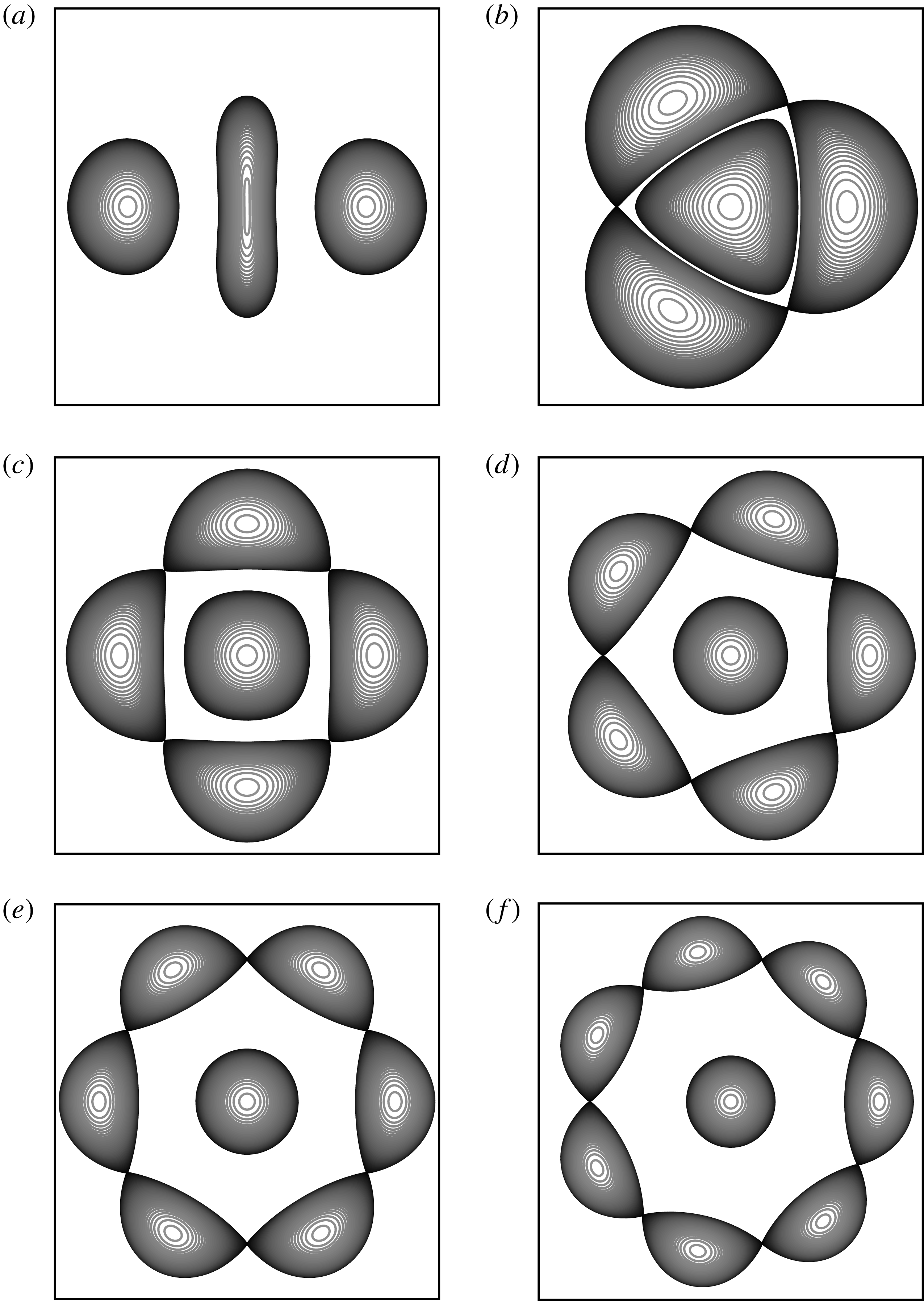
Figure 13 shows the vortex equilibria for the ( $m+1$ )-vortex problem when $d=0$ and $\unicode[STIX]{x1D6FC}=-1$ . Recall that, except for $m=3$ , the associated point vortex arrays are unstable. The general shape of the equilibria is qualitatively similar to the shape of the two-dimensional equilibria obtained by Kizner et al. (Reference Kizner, Khvoles and McWilliams2007) and the vortex arrays obtained experimentally by Trieling, van Heijst & Kizner (Reference Trieling, van Heijst and Kizner2010). It should be noted that we have not been able to reach an end point in the case $m=2$ despite numerous attempts. Importantly, the algorithm requires that we fix a distance between two points discretising the vortices during the iterative procedure to determine the equilibrium. When the equilibrium is reached, this distance is reduced and the procedure is resumed for this new distance. As mentioned previously, not all distances vary monotonically along the branch of solutions, and we may need to describe the solution branch piece by piece, adapting the adequate distance to be fixed. In the case $m=2$ , we were not able to find a convenient distance to be fixed that would allow one to go further along the branch. A new approach may be required in this case.

The presence of an opposite-signed vortex in the centre of the structure changes the topology of the streamlines, hence the shape of the equilibria. This difference with the $m$ -vortex problem becomes less noticeable for large $m$ , as the vortices remain far from the central vortex even at the end point of the branch. However, the peripheral vortices tend to be thinner in the radial direction when the opposite-signed central vortex is present. It is, however, important to stress that these qualitatively similar vortex shapes have fundamentally different stability properties.

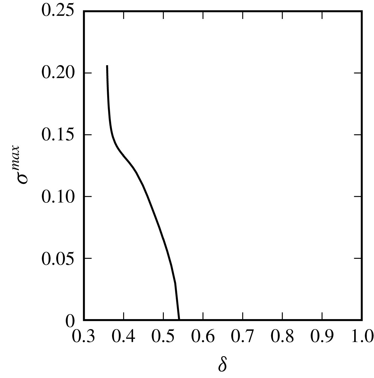
Figure 14 shows the maximum growth rate $\unicode[STIX]{x1D70E}^{max}$ for the ( $3+1$ )-vortex problem with $d=0$ and $\unicode[STIX]{x1D6FC}=-1$ . We do not show results for the other values of $m$ , as they are all unstable for all distances. Indeed, these configurations are all unstable to at least displacement modes as found for the point vortices. The linear stability of the finite-volume vortices confirmed this. The case $m=3$ is the only one which is linearly stable to displacement modes. Again, we see that deformation modes can destabilise the equilibrium if the vortices are close enough together. Recall that vortices at equilibrium are more deformed as they are closer together.

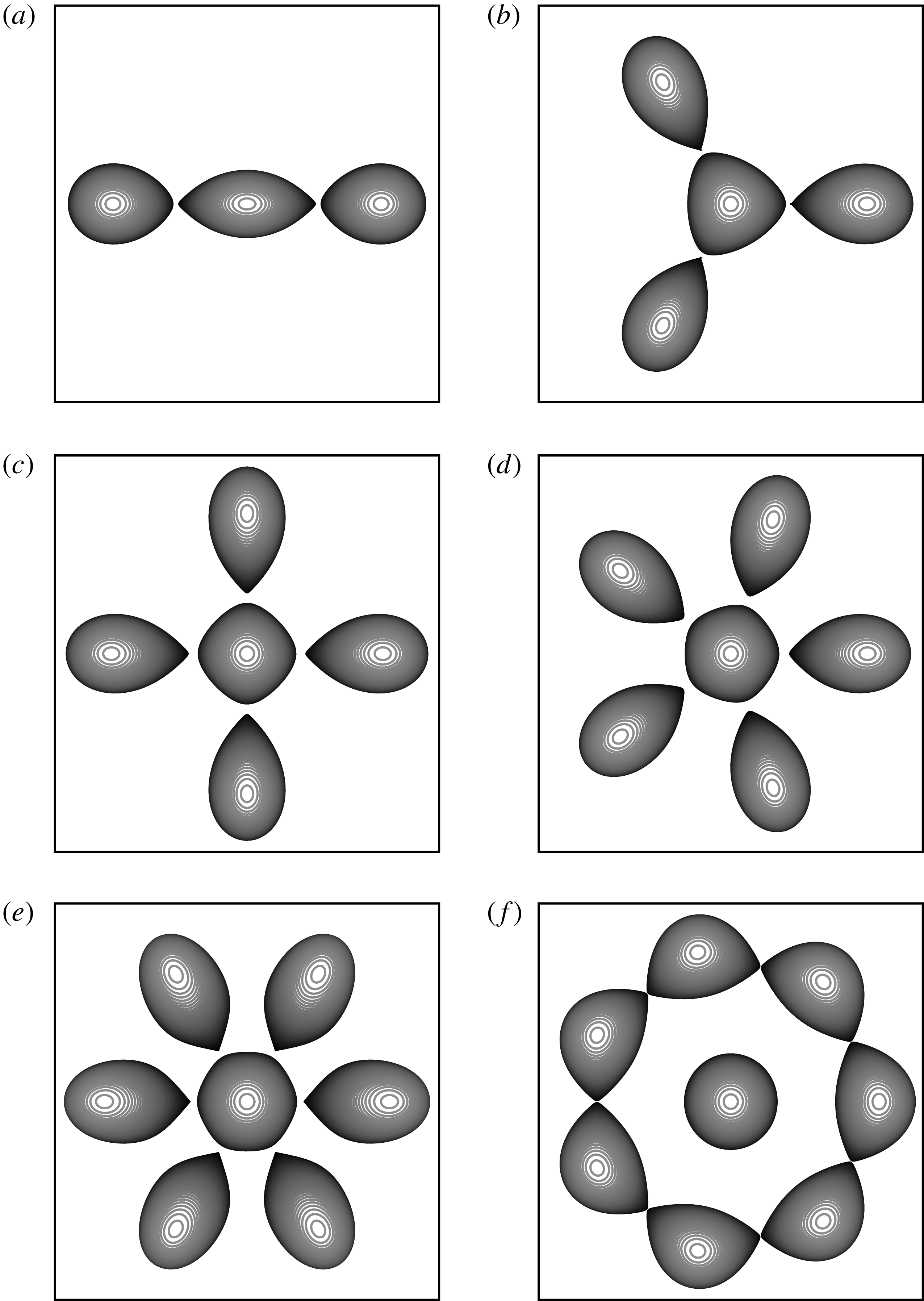
Finally, figure 15 illustrates the equilibria at the end point of the solution branches for the ( $m+1$ )-vortex problem with $d=0$ and $\unicode[STIX]{x1D6FC}=1$ . Owing to the presence of the central like-signed vortex, the vortex exhibits a sharp inner edge for $m\leqslant 6$ . Note that, for $m>6$ , the distance between two neighbouring peripheral vortices is less than the distance between these vortices and the central vortex. In these cases, the peripheral vortices interact more strongly with their neighbours on the ring. This explains the change in the shape of the equilibria.

Figure 13.

Top view of the vortex bounding contours to the ( $m+1$ )-vortex equilibria at the end of the solution branch where the vortices touch (except for $m=2$ in (a), where this state could not be obtained numerically). The central vortex and the peripheral vortices have opposite-signed PV. The grey scale indicates the height of the contour: lighter grey contours are nearer the top.

Figure 14.

Maximum growth rate $\unicode[STIX]{x1D70E}^{max}$ of instability versus the inner gap $\unicode[STIX]{x1D6FF}$ for the finite-volume ( $m+1$ )-vortex problem for $m=3$ where the central vortex and the peripheral vortices have opposite sign.

Figure 15.

Top view of the vortex bounding contours to the ( $m+1$ )-vortex equilibria at the end of the solution branch where the vortices touch. The central vortex and the peripheral vortices have the same PV. The grey scale indicates the height of the contour: lighter grey contours are nearer the top.

Figure 16.

Maximum growth rate $\unicode[STIX]{x1D70E}^{max}$ of instability versus the inner gap $\unicode[STIX]{x1D6FF}$ for the finite-volume ( $m+1$ )-vortex problem where the central vortex and the peripheral vortices have the same sign for $m=3$ (solid black), $4$ (dotted black), $5$ (dashed-dotted black), $6$ (solid red) and $7$ (dotted red).

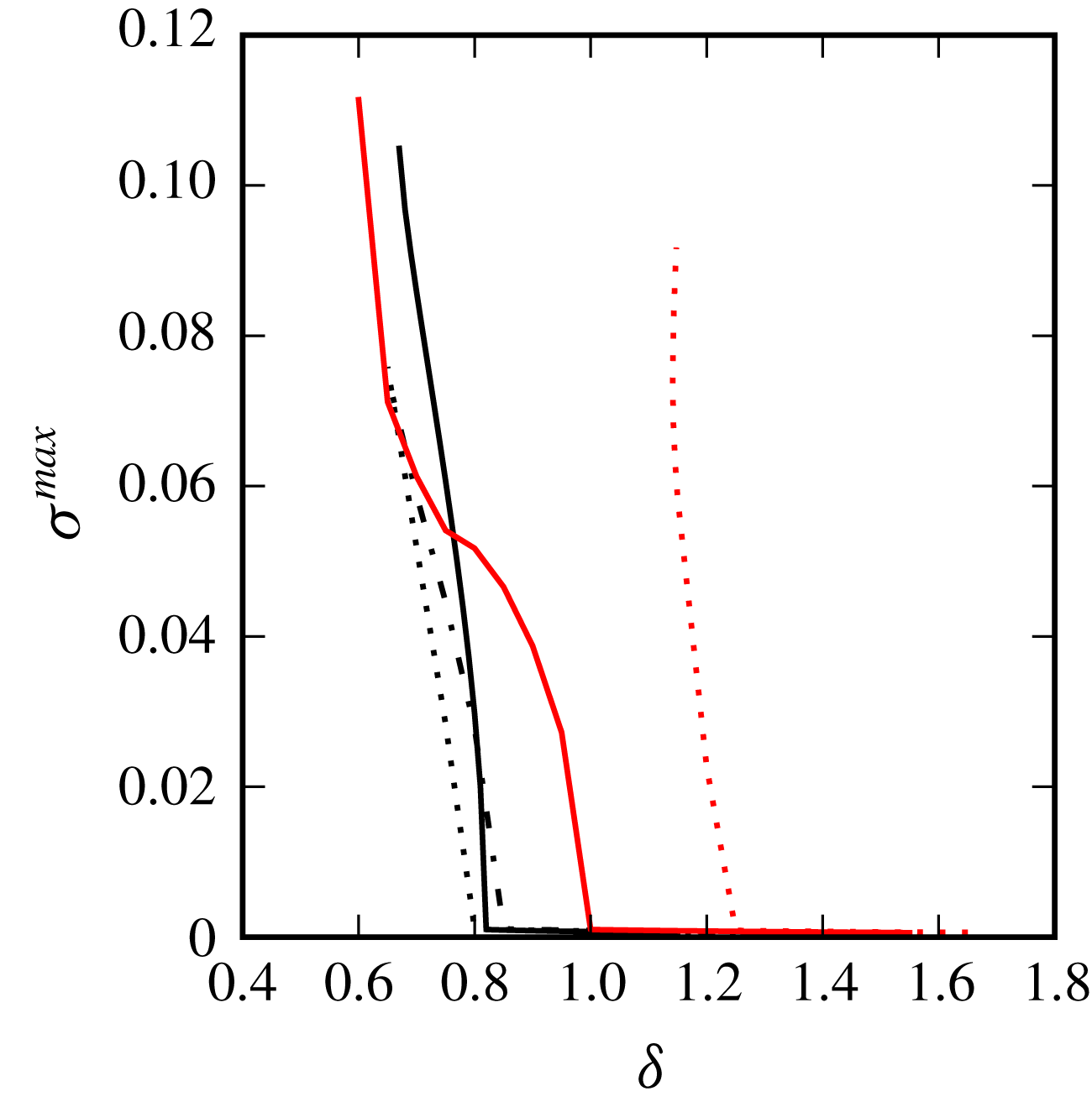
The maximum growth rate $\unicode[STIX]{x1D70E}^{max}$ of the unstable modes versus $\unicode[STIX]{x1D6FF}$ is shown in figure 16. Again, unstable modes are obtained for $\unicode[STIX]{x1D6FF}$ less than a threshold for all $m$ . The weak unstable mode observed for the ( $3+1$ ) point vortex system for $d=0$ and $\unicode[STIX]{x1D6FC}=1$ is not clearly captured for the finite-volume problem. We conjecture that, as seen for the six-vortex problem, the deformation of the vortices, hence their capacity to adapt to the external shear, weakens the instability. The growth rate of the instability is of the order of the background numerical noise.

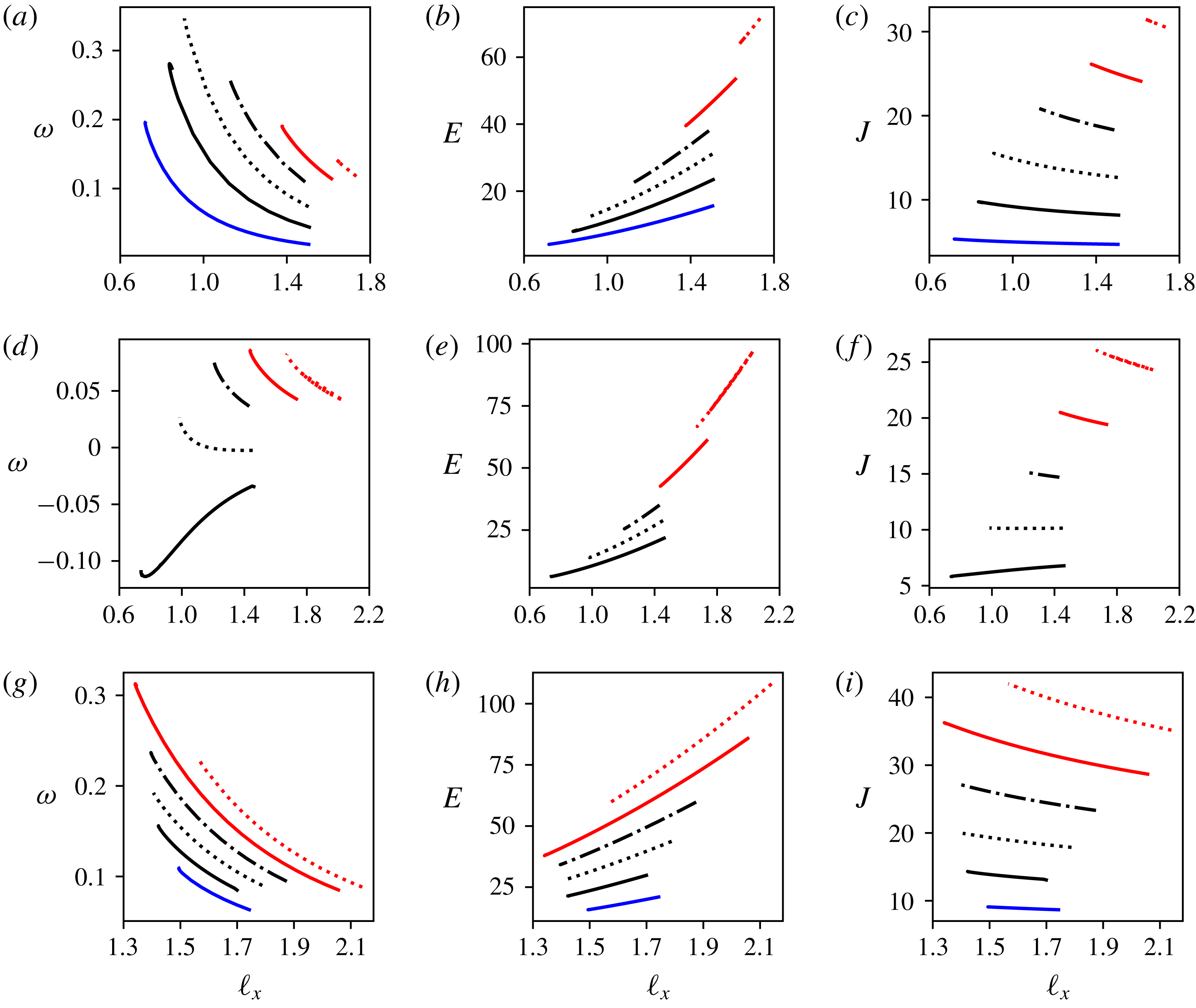
For the sake of completeness, one can also calculate two of the fundamental invariants of the equilibria, namely their total energy $E$ and their angular impulse $J$ , defined by

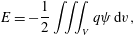(4.1) $$\begin{eqnarray}\displaystyle & \displaystyle E=-{\displaystyle \frac{1}{2}}\iiint _{V}q\unicode[STIX]{x1D713}\,\text{d}v, & \displaystyle\end{eqnarray}$$

(4.2) $$\begin{eqnarray}\displaystyle & \displaystyle J={\displaystyle \frac{1}{2}}\iiint _{V}q(x^{2}+y^{2})\,\text{d}v. & \displaystyle\end{eqnarray}$$

A summary of the results is presented in figure 17. For the two-vortex problem, the margin of stability has been observed empirically to coincide with the maximum of $E$ and minimum of $J$ versus the distance separating the vortices (see Reinaud & Dritschel Reference Reinaud and Dritschel2002, Reference Reinaud and Dritschel2005). The fact that the combined extrema can be associated with the onset of instability has been justified by Safman (Reference Safman1992) using Kelvin’s variational principle. The condition is a sufficient but not necessary condition. We have not found a systematic match between the onset of instability and the coincidence of extrema for $E$ and $J$ for $m>2$ . It should be noted that such a match should not be expected, at least for the displacement mode, as its origin is independent of the distance separating the vortices. For almost all cases, the rotation rate $\unicode[STIX]{x1D714}$ and the energy $E$ increase as the vortices are closer to one another, hence their interaction is stronger. On the other hand, $J$ decreases with the distance, as $J$ is associated with a volume integral of PV weighted by distance to the system centre squared. Only for the case $m=3$ and $d=0$ , $\unicode[STIX]{x1D6FC}=-1$ do these trends differ. In this case the peripheral vortices are close to the highly deformed opposite-signed central vortex. This central vortex dominates the overall rotation (which becomes clockwise) and its contribution to the angular impulse is negative.

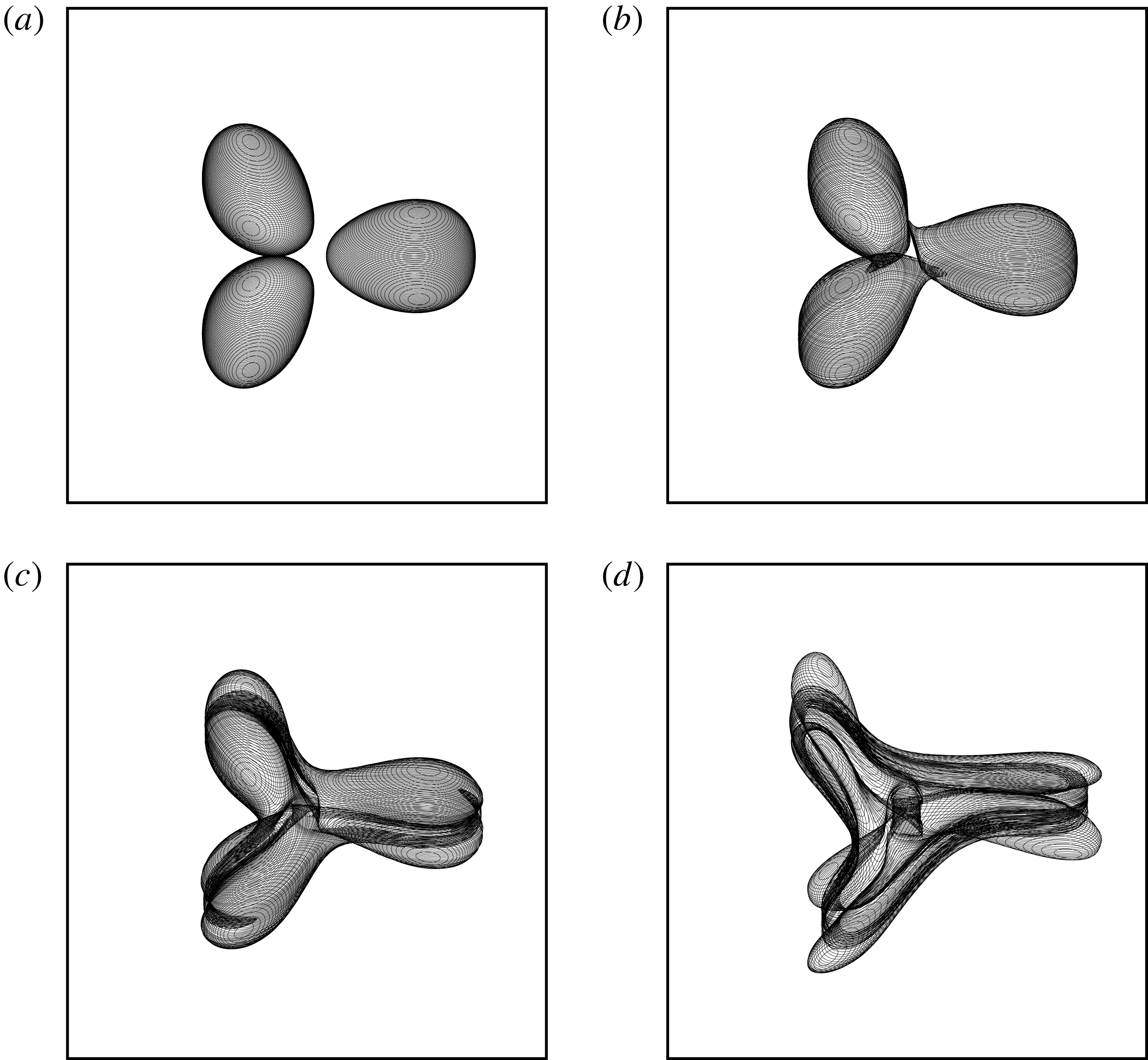
We next illustrate the nonlinear evolution of unstable equilibria for the three categories of vortex arrays. We start with an example of the three-vortex problem. The equilibrium corresponds to a state with an innermost gap $\unicode[STIX]{x1D6FF}=0.16$ and the maximum growth rate of instability is $\unicode[STIX]{x1D70E}^{max}=0.037$ . Results obtained with the Lagrangian contour dynamics method are presented in figure 18. The equivalent equilibrium with point vortices is linearly stable, indicating that there is no unstable displacement mode. The instability is associated with the deformation of the vortices. We do not force the instability but simply let it grow from pseudo-random numerical errors. For numerical efficiency the number of nodes discretising the contours of the equilibrium ( $n_{p}=4n_{c}$ ) is reduced while maintaining high accuracy. This is done by ‘renoding’ the contours, which is part of contour surgery with standard set-up parameters. This procedure is enough to introduce a small perturbation on the vortex shape. Figure 18 shows the vortices in the reference frame steadily rotating with the equilibrium. Therefore, any motion observed in this reference frame represents a departure from equilibrium. The vortices remain at equilibrium for a long period of time, while the deformation slowly grows from the low numerical noise. By $t=22$ , the innermost edges of the vortices have deformed and have formed bridges which connect them to the neighbouring vortex to their right (in the direction of rotation of the structure). This deformation is qualitatively similar to the one associated with the merger of a pair of like-signed vortices (see Reinaud & Dritschel Reference Reinaud and Dritschel2002). As the flow develops, the merged vortex forms a complex structure which resembles a three-blade propeller. Some PV from the central layers converges to the centre of the structure. To conserve the angular impulse $J$ , some PV from the lower and upper layers of the vortices is ejected away from the centre of the structure. These will turn into filaments and small-scale debris in the late evolution of the flow.

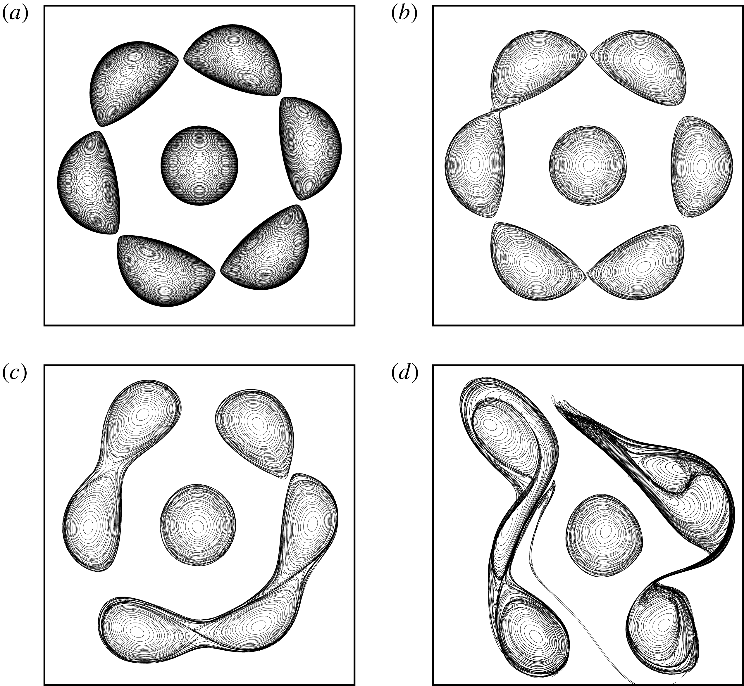
The second illustration of the nonlinear evolution of the equilibria concerns an unstable ( $6+1$ )-vortex equilibrium with $d=0$ and $\unicode[STIX]{x1D6FC}=-1$ . Recall that such a vortex array is sensitive to a displacement mode. Results obtained with the Lagrangian contour dynamics method are shown in figure 19. Here, the distance $\unicode[STIX]{x1D6FF}$ between the peripheral vortex innermost edge and the centre of the central vortex is $\unicode[STIX]{x1D6FF}=1.08$ and the most unstable mode has a growth rate $\unicode[STIX]{x1D70E}^{max}=0.12$ . We first observe that the vortices indeed move. Some vortices get closer together, creating a larger gap with their other neighbouring vortex on the ring. The straining field changes as the vortices depart from their equilibrium. The vortices thus start to deform. The vortices which have got closer together merge to form larger structures. These structures are not stable and can further interact and/or break back into much deformed secondary structures. This resembles instances of partial merger observed during the interaction between two vortices (see Reinaud & Dritschel Reference Reinaud and Dritschel2002).

Figure 17.

Global diagnostics for the equilibrium state: rotation rate $\unicode[STIX]{x1D714}$ , total energy $E$ and angular impulse $J$ versus $\ell _{x}$ , the distance between the centroid of the peripheral vortices and the centre of the ring, for $m=2$ (solid blue), $m=3$ (solid black), $m=4$ (dotted black), $m=5$ (dashed-dotted black), $m=6$ (solid red) and $m=7$ (dotted red); and for the $m$ -vortex problem (a–c), the ( $m+1$ )-vortex problem with $d=0$ , $\unicode[STIX]{x1D6FC}=-1$ (d–f) and the ( $m+1$ )-vortex problem with $d=0$ , $\unicode[STIX]{x1D6FC}=1$ (g–i).

Figure 18.

Evolution of the vortex bounding contours for an unstable $(\unicode[STIX]{x1D70E}^{max}=0.037)$ array of three vortices in mutual equilibrium for $\unicode[STIX]{x1D6FF}=0.16$ at $t=0$ , $22$ , $24$ and $27.5$ . The vortex bounding contours are viewed orthographically at an angle of $45^{\circ }$ from the vertical.

Figure 19.

Evolution of the vortex bounding contours for an unstable ( $\unicode[STIX]{x1D70E}^{max}=0.12$ ) array of six peripheral vortices and an opposite-signed central vortex ( $\unicode[STIX]{x1D6FC}=-1$ ) with $d=0$ , in mutual equilibrium for $\unicode[STIX]{x1D6FF}=1.08$ at $t=0$ , $12$ , $16$ and $21$ . The vortex bounding contours are viewed from the top.

Figure 20.

Evolution of the vortex bounding contours for an unstable ( $\unicode[STIX]{x1D70E}^{max}=0.076$ ) array of four peripheral vortices and a like-signed central vortex ( $\unicode[STIX]{x1D6FC}=1$ ) with $d=0$ , in mutual equilibrium for $\unicode[STIX]{x1D6FF}=0.16$ at $t=10$ , $14$ , $20$ and $24$ . The vortex bounding contours are viewed from the top.

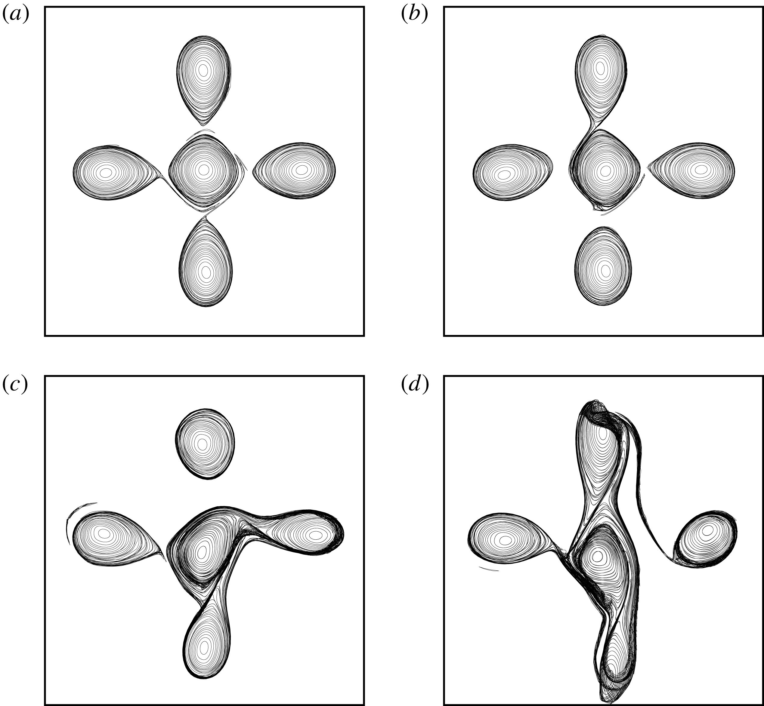
Finally, we consider an example of unstable ( $4+1$ )-vortex equilibrium with $d=0$ and $\unicode[STIX]{x1D6FC}=1$ with $\unicode[STIX]{x1D6FF}=0.16$ and $\unicode[STIX]{x1D70E}^{max}=0.076$ . The equivalent point vortex equilibrium is linearly stable. Results obtained with the Lagrangian contour dynamics method are presented in figure 20. In this case, the instability is associated with the deformation of the vortices. The sharp inner edge of the peripheral vortices elongates and a filament of PV is shed near the edge of at least one vortex. This filament is wrapped around the central vortex. This in turn breaks the symmetry of the flow. As the vortices deform, some of the peripheral vortices strongly interact with the central vortex in an asymmetric way. This is followed by a series of partial mergers, and breaking into secondary vortices. In the latter two cases the central vortex remains near the centre of the domain at least for the duration of the simulation. This is due to conservation of the linear and angular impulses, as overall the system must remain anchored to the centre of the domain.