I. INTRODUCTION
According to Foster theory, reactance of passive and lossless single-port network increases with frequency and this was first proved by Foster in 1924 [Reference Foster1]. If the reactance or susceptance of an element decreases with frequency, this circuit represents non-Foster element and behaves as negative capacitor or inductor. The concept of non-Foster circuit is not new at all. It is based on the concept of negative impedance converter (NIC) that was proposed in the 1950s by Linvill [Reference Linvill2].
Non-Foster circuits are widely used to improve the performance and bandwidth of various circuits. The applications include matching of electrically small antenna [Reference Sussman-Fort and Rudish3], active dispersion-less metamaterial [Reference Hrabar, Krois, Bonic and Kiricenko4], increasing the tuning range of a varactor diode by using a negative capacitance [Reference Kolev, Delacressonniere and Gautier5] and enhancement of gain of distributed amplifiers with negative capacitance [Reference Ghadiri and Moez6]. The stability of non-Foster circuits has been mentioned as the greatest practical problem [Reference Stearns7]. These circuits are based on positive feedback structure and this may cause system instability due to the change of operating point or other parameters of circuits. For this reason, modeling and analysis of non-Foster circuits and their stability have a great importance. Investigation of non-Foster circuits’ stability is generally performed on the basis of small-signal and linear model that may not be appropriate in all cases [Reference Stearns7–Reference Rengarajan and White11].
Modeling and nonlinear analysis of circuit in the time domain are used for achieving transient response of the circuit that investigates the stability and the actual behavior of the circuit while other analysis approaches like harmonic balance (HB) are only used to analyze the steady state response of circuit, which for the instability condition the response never tends to it. In this paper, modeling and analysis of nonlinear non-Foster elements in the time domain are investigated and the results are compared and evaluated with the commercial software, which shows a good compatibility.
II. NON-FOSTER STRUCTURE
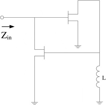
The structure of a NIC used to create the negative capacitance, is shown in Fig. 1 [Reference Kolev, Delacressonniere and Gautier5].
The structure of NIC creating a negative capacitance.

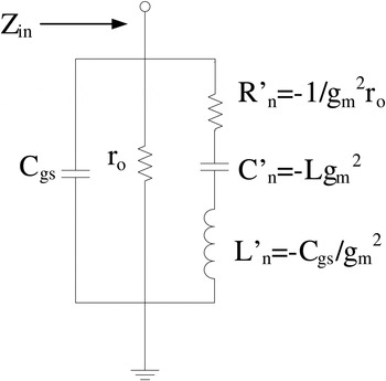
By considering the linear and small-signal model of transistors, the equivalent circuit of NIC circuit is obtained as shown in Fig. 2. The equivalent negative capacitance (C n ) based on the heart of the transistor (g m ), ignoring the effects of the parasitic elements (r 0 and C gs ) is expressed as [Reference Kolev, Delacressonniere and Gautier5]:
 $$C_n = - g_m^2 L,$$
Equivalent impedance of the negative capacitor converter.

In literatures and recent papers [Reference Stearns7–Reference Rengarajan and White11], analysis of non-Foster circuits and their stability are generally based on linear model, while with increasing the signal level and time-varying operating point, the linear model is invalid and the stability analysis may be void, hence the necessity of nonlinear analysis of non-Foster circuits and their stability based on time domain transient behavior of the circuit, are felt. These are argued in the rest of the paper.
III. NONLINEAR MODELING OF NON-FOSTER CIRCUITS
The first step in analysis of a structure, is modeling of its elements. Here, the introduced negative capacitance converter includes two field-effect transistors (FETs) and one inductance (L). The famous nonlinear models such as Curtice2, Curtice3, Statz, TOM, Tajima, Advanced Curtice Model, etc. are used to model the performance of FETs based on the various parameters. In this paper, based on Curtice2 model and considering the heart of transistor i.e. nonlinear current source, the behavior of the circuit will be discussed. In the Curtice2 model, the nonlinear current source (I ds ) is described according to voltages of the transistor (2), knowing that if the V gs is smaller than V T0 then the current source is zero [Reference Curtice12].
 $$I_{ds}\left( {V_{gs},V_{ds}} \right) = \beta \left( {V_{gs} - V_{T0}} \right)^2\left( {1 + \lambda V_{ds}} \right)\tanh \left( {\alpha V_{ds}} \right).$$
Mutual conductance (g m ) and output conductance (g ds ) are obtained in the following expressions [Reference Curtice12].
 $$g_m = \displaystyle{{\partial I_{ds}} \over {\partial V_{gs}}} = I_{ds}\left( {\displaystyle{2 \over {V_{gs} - V_{T0}}}} \right),$$
 $$\eqalign{g_{ds} & = \displaystyle{{\partial I_{ds}} \over {\partial V_{ds}}} = \beta \left( {V_{gs} - V_{T0}} \right)^2\ \lambda \tanh \left( {\alpha V_{ds}} \right) \cr & \quad+ \beta \left( {V_{gs} - V_{T0}} \right)^2\ \left( {1 + \lambda V_{ds}} \right)\left( {\displaystyle{\alpha \over {{\cosh} ^2(\alpha V_{ds})}}} \right).}$$
In these equations α, β, and λ are fixed parameters of the model and V
T0 is the pinch-off voltage of transistor. The term
 $(V_{gs} - V_{T0})^2$
describes I
ds
with respect to V
gs
as a quadratic polynomial and this is why this model is called Curtice2 [Reference Curtice12].
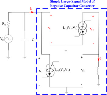
The large-signal model of the NIC, as shown in Fig. 3, is obtained based on simple large-signal model of FETs. Other parasitic elements such as capacitors are ignored. The time-domain analysis is used to analyze the nonlinear performance of NIC.
Large-signal model of NIC with placing the capacitor C to stabilize performance of circuit.

The capacitor C is added in the input of NIC, to prevent instability of circuit. The time constant of equivalent resistor–capacitor (RC) circuit is calculated as:
 $$\tau = R(C + C_n).$$
The positive value of the time constant and the total capacitor of circuit is the necessary condition of stability of circuit.
To analyze the circuit based on Fig. 3, the state variables including the inductor current (I L ) and the capacitor voltage (V 1) are achieved based on the circuit relations (6–8).
 $$V_2 = L\displaystyle{{dI_L} \over {dt}},$$
 $$I_L = - I_{NL}(V_1,V_2),$$
 $$C\displaystyle{{dV_1} \over {dt}} + \displaystyle{{V_1 - V_g} \over {R_g}} + I_{NL}(V_2,V_1) = 0.$$
By considering these relations and analyzing the circuit, the behavior of NIC is modeled as a negative nonlinear capacitor that is determined according to the voltage applied to it.
IV. NONLINEAR ANALYSIS OF NEGATIVE CAPACITANCE CONVERTER IN THE TIME DOMAIN
In this section we focus on nonlinear analysis of NIC in time domain based on the obtained relations and nonlinear model of FETs. The behavior of negative capacitance and stability of circuit would be examined from the transient response.
In the time-domain analysis, based on the relations of circuits and dividing the total analysis time to Δt steps, according to the maximum existing frequency, the parameters of circuit (V 1, V 2, I 1, and I L ) are obtained in each step from parameters of current and previous steps. In the proposed method, it is assumed that the differences of parameters in each step are small. The parameters in the current step are achieved from their previous values that are mentioned in the relations (9–13).
 $$t(i) = (i - 1)\Delta t,$$
 $$V_1^i = V_1^{i - 1} + \Delta v_1,$$
 $$V_2^i = V_2^{i - 1} + \Delta v_2,$$
 $$I_1^i = I_1^{i - 1} + \Delta i_1,$$
 $$I_L^i = I_L^{i - 1} + \Delta i_L.$$
Nonlinear current source values i.e. I NL1 and I NL2 are obtained at every step from the applied voltages V 1 and V 2 and bias voltages V GS and V DS from (14, 15).
 $$\eqalign{I_{NL1}^i & = I_{NL}\,(V_{GS} + V_2^i, V_{DS} + V_1^i ) \cr & = I_{NL}\,(V_{GS} + V_2^{i - 1} + \Delta v_2,V_{DS} + V_1^{i - 1} + \Delta v_1),}$$
 $$\eqalign{I_{NL2}^i & = I_{NL}\,(V_{GS} + V_1^i, V_{DS} + V_2^i ) \cr & = I_{NL}\,(V_{GS} + V_1^{i - 1} + \Delta v_1,V_{DS} + V_2^{i - 1} + \Delta v_2).}$$
Assuming small variations of V 1 and V 2 (Δv 1 and Δv 2) in each step, the Taylor expansion is used to obtain the nonlinear current source relations (16, 17). G m and G d are time-varying parameters that are changed in each step.
 $$\eqalign{I_{NL1}^i & = I_{NL}\,(V_{GS} + V_2^{i - 1}, V_{DS} + V_1^{i - 1} ) + \displaystyle{{\partial I_{NL}} \over {\partial V_2}}\Delta v_2 \cr & \quad+ \displaystyle{{\partial I_{NL}} \over {\partial V_1}}\Delta v_1 = I_{NL1}^{i - 1} + G_{m1}^{i - 1} \Delta v_2 + G_{d1}^{i - 1} \Delta v_1,}$$
 $$\eqalign{I_{NL2}^i &= I_{NL}(V_{GS} + V_1^{i - 1}, V_{DS} + V_2^{i - 1} ) + \displaystyle{{\partial I_{NL}} \over {\partial V_1}}\Delta v_1 \cr & \quad + \displaystyle{{\partial I_{NL}} \over {\partial V_2}}\Delta v_2 = I_{NL2}^{i - 1} + G_{m2}^{i - 1} \Delta v_1 + G_{d2}^{i - 1} \Delta v_2.}$$
By using linear time-varying model of current sources and the negative capacitor converter circuit equations, relations (6–8) are re-written in inter-step (i − 1/2) between i, i − 1 and the equations for the time-domain analysis of circuit are provided (18–20). The DC bias currents are supplied by the feeding networks, which are not shown to prevent complexity of network, but their effects are seen by subtracting I DC from current sources in drain nodes.
 $$\eqalign{V_2 &= L\displaystyle{{dI_L} \over {dt}} \cr V_2^{i - 1/2} &= \displaystyle{{V_1^i + V_1^{i - 1}} \over 2} = V_2^{i - 1} + \displaystyle{{\Delta v_2} \over 2} = L\displaystyle{{\Delta i_L} \over {\Delta t}}, \cr \Delta v_2 &= 2L\displaystyle{{\Delta i_L} \over {\Delta t}} - 2V_2^{i - 1}} $$
 $$\eqalign {C\displaystyle{{dV_1} \over {dt}} &+ \displaystyle{{V_1 - V_g} \over {R_g}} + I_{NL}(V_2,V_1) - I_{DC} = 0, \cr C\displaystyle{{V_1^i - V_1^{i - 1}} \over {\Delta t}} &+ \displaystyle{{(V_1^i + V_1^{i - 1} ) - (V_g^i + V_g^{i - 1} )} \over {2R_g}} \cr & + I_{NL}^{i - 1/2} (V_2,V_1) - I_{DC} = 0 \cr C\displaystyle{{\Delta v_1} \over {\Delta t}} &+ \displaystyle{{(2V_1^{i - 1} + \Delta v_1) - (V_g^i + V_g^{i - 1} )} \over {2R_g}} + I_{NL1}^{i - 1} \cr & \quad+ G_{m1}^{i - 1} \Delta v_2/2 + G_{d1}^{i - 1} \Delta v_1/2 - I_{DC} = 0 \cr C\displaystyle{{\Delta v_1} \over {\Delta t}} &+ \displaystyle{{(2V_1^{i - 1} + \Delta v_1) - (V_g^i + V_g^{i - 1} )} \over {2R_g}} + I_{NL1}^{i - 1} \cr & \quad + G_{m1}^{i - 1} \left( {2L\displaystyle{{\Delta i_L} \over {\Delta t}} - 2V_2^{i - 1}} \right)\Big/2 \cr & \quad+ G_{d1}^{i - 1} \Delta v_1/2 - I_{DC} = 0,} $$
 $$\eqalign{I_L &= - I_{NL}(V_1,V_2) \cr I_L^{i - 1} & + \displaystyle{{\Delta i_L} \over 2} + I_{NL}^{i - 1/2} (V_1,V_2) - I_{DC} = 0 \cr I_L^{i - 1} & + \displaystyle{{\Delta i_L} \over 2} + I_{NL2}^{i - 1} + G_{m2}^{i - 1} \Delta v_1/2 + G_{d2}^{i - 1} \Delta v_2/2 - I_{DC} = 0 \cr I_L^{i - 1} &+ \displaystyle{{\Delta i_L} \over 2} + I_{NL2}^{i - 1} + G_{m2}^{i - 1} \Delta v_1/2 \cr &+ G_{d2}^{i - 1} \left( {2L\displaystyle{{\Delta i_L} \over {\Delta t}} - 2V_2^{i - 1}} \right)/2 - I_{DC} = 0.}$$
Using these relations, Δv 1 and Δi L at each step are achieved based on voltage, current and other time-varying parameters in the previous steps, the corresponding matrix equations are shown in (21, 22).
 $$\matrix{ {\left[ {\matrix{ {\displaystyle{C \over {\Delta t}} + \displaystyle{1 \over {2R_g}} + G_{d1}^{i - 1} /2} & {G_{m1}^{i - 1} \displaystyle{L \over {\Delta t}}} \cr {G_{m2}^{i - 1} /2} & {\displaystyle{1 \over 2} + G_{d2}^{i - 1} \displaystyle{L \over {\Delta t}}} \cr}} \right]\left[ {\matrix{ {\Delta v_1} \cr {\Delta i_L} \cr}} \right]} \cr { = - \left[ {\matrix{ {\displaystyle{{2V_1^{i - 1} - (V_g^i + V_g^{i - 1} )} \over {2R_g}} + I_{NL1}^{i - 1} - G_{m1}^{i - 1} V_2^{i - 1} - I_{DC}} \cr {I_L^{i - 1} + I_{NL2}^{i - 1} - G_{d2}^{i - 1} V_2^{i - 1} - I_{DC}} \cr}} \right]}, \cr} $$
 $$\eqalign{&{\left[{\matrix{ {\Delta v_1} \cr {\Delta i_L} \cr}} \right] = - {\left[ {\matrix{ {\displaystyle{C \over {\Delta t}} + \displaystyle{1 \over {2R_g}} + G_{d1}^{i - 1} /2} & {G_{m1}^{i - 1} \displaystyle{L \over {\Delta t}}} \cr {G_{m2}^{i - 1} /2} & {\displaystyle{1 \over 2} + G_{d2}^{i - 1} \displaystyle{L \over {\Delta t}}} \cr}} \right]}^{ - 1}} \cr & {\left[ {\matrix{ {\displaystyle{{2V_1^{i - 1} - (V_g^i + V_g^{i - 1} )} \over {2R_g}} + I_{NL1}^{i - 1} - G_{m1}^{i - 1} V_2^{i - 1} - I_{DC}} \cr {I_L^{i - 1} + I_{NL2}^{i - 1} - G_{d2}^{i - 1} V_2^{i - 1} - I_{DC}} \cr}} \right]}.}$$
V. ANALYSIS RESULTS IN THE TIME DOMAIN
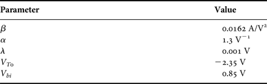
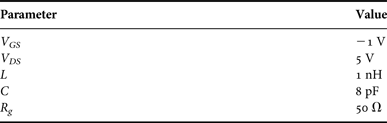
According to the proposed method for modeling negative capacitance converter in the time domain as the linear time-varying model, in this section we analyze the behavior of a negative capacitance in the time domain and compare the results with those of commercial software. They have good agreement with each other and the proposed method is validated. Parameters of nonlinear model of FETs are shown in Table 1. In this model, the parameters of the nonlinear current source as the heart of transistor are considered and other parasitic elements are ignored [Reference Khoshniyat, Moradi, Abdipour and Afrooz13].
Parameters of curtice 2 model.

Other parasitic elements such as capacitors are ignored.
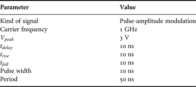
In Table 2, the values of parameters of circuit such as DC bias voltages, inductor and capacitor are shown. The parameters of input signal are presented in Table 3.
Negative capacitance converter circuit parameters.

Specifications of the input signal.

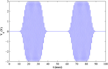
The input signal (V g ) with 3 V peak voltage and other specifications as detailed in Table 3, is shown in Fig. 4.
The input signal, the modulated pulse with 1 GHz carrier frequency and 3 V peak voltage.

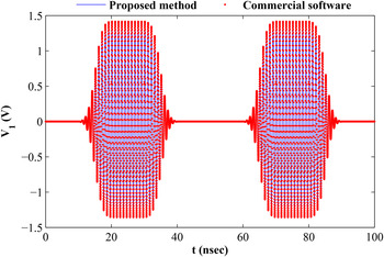
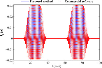
The results of circuit analysis with linear time-varying model are shown in Figs 5 and 6, which are compared with the results of commercial software that have a good agreement with each other and the proposed method is validated. These results are voltage and current at the input of negative capacitance converter (V 1 and I 1), that the nonlinearity can be seen well in them, especially in I 1, due to the large amplitude of the input signal.
The voltage at the input of negative capacitance converter (V 1) that is analyzed by the proposed method and commercial software.

The current at the input of negative capacitance converter (I 1) that is analyzed by the proposed method and commercial software.

By validating the linear time-varying model for analysis of non-Foster capacitors, the proposed approach is used in modeling and extraction of the negative capacitor.
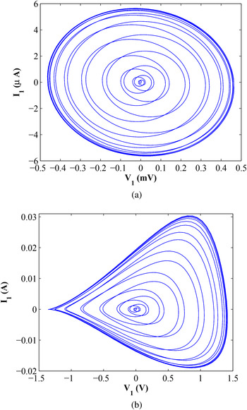
Lissajous curve (
 $x = V_1(t)$
and
 $y = I_1(t)$
) is shown in Fig. 7 that is obtained by eliminating the time as the independent variable. The outer rings of the curve, which were repeated several times, are the steady state response of pulses while the central parts of ring belong to the rise time and fall time of the pulse. The direction of curve as a function of time is counter-clockwise that represent the circuit function as a negative capacitance. In Fig. 7(a), the curve for the 1 mV peak voltage plotted while the peak voltage is 3 V in Fig. 7(b), and nonlinearity of circuit is well evident with increasing the signal amplitude.
Lissajous curve (
 $x = V_1(t)$
and
 $y = I_1(t))$
of the negative capacitance converter, (a) input signal with the 1 mV peak voltage, (b) input signal with the 3 V peak voltage.

VI. EXTRACTION OF NONLINEAR NEGATIVE CAPACITOR FOR STABILITY STUDY
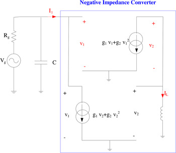
As shown in Fig. 8, the simple second order model of current source of FETs is used in analysis of NIC. The current source (Ids) is represented by:
 $$I_{ds} = g_1v_{gs} + g_2v_{gs}^2, $$
 $$g_1 = \displaystyle{{2I_{ds}} \over {V_{gs} - V_{T0}}},$$
 $$g_2 = \displaystyle{{I_{ds}} \over {{(V_{gs} - V_{T0})}^2}}.$$
Large-signal model of NIC with simple second order nonlinear model of FETs.

By applying circuit relations, based on Kirchhoff's current law and Kirchhoff's voltage law, and considering second order representation of I ds , the I 1 is obtained by (28). Assuming a capacitive behavior of NIC (28), the nonlinear model of negative capacitor is achieved as (30).
 $$I_L = - (g_1v_1 + g_2v_1^2 ),$$
 $$v_2 = L\displaystyle{{dI_L} \over {dt}} = - L(g_1 + 2g_2v_1)\displaystyle{{dv_1} \over {dt}},$$
 $$\eqalign{I_1 & = (g_1v_2 + g_2v_2^2 ) = - Lg_1(g_1 + 2g_2v_1)\displaystyle{{dv_1} \over {dt}} \cr & \quad+ L^2g_2(g_1^2 + 4g_1g_2v_1 + 4g_2^2 v_1^2 )\left( {\displaystyle{{dv_1} \over {dt}}} \right)^2,}$$
 $$I_1 = C\left( {v_1,\displaystyle{{dv_1} \over {dt}}} \right)\left( {\displaystyle{{dv_1} \over {dt}}} \right),$$
 $$C\left( {v_1,\displaystyle{{dv_1} \over {dt}}} \right) = C_0 + C_1v_1 + \left[ {B_0 + B_1v_1 + B_2v_1^2} \right]\displaystyle{{dv_1} \over {dt}}.$$
In this section, by using the results of the analysis based on proposed method in time domain, the nonlinear negative capacitor is extracted, according to voltage and other parameters (31, 32).
 $$C(t) = \displaystyle{{dq(t)} \over {dv(t)}}, $$
 $$q(t) = \int_0^t i(t)dt.$$
With certain considerations in numerical calculation such as avoiding divide by zero (too small dv(t)) and considering the neighborhood
 $(t - h,t + h)$
, Δq, Δv, and C
n
(t) are calculated according to equations (33–36).
 $$\Delta v(t) = V(t + h) - V(t - h),$$
 $$\Delta q(t) = \int_{t - h}^{t + h} i(t)dt,$$
 $$C_n(t) = \displaystyle{{\Delta q(t)} \over {\Delta v(t)}}, $$
 $$V(t) = \displaystyle{{[V(t + h) + V(t - h)]} \over 2}.$$
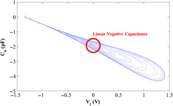
By eliminating the time as the independent variable, the curve of V(t) − C(t) is obtained, which is shown in Fig. 9, like the curve of V-I, middle rings belong to rise and fall times of pulse while outer rings belong to the steady state response of the circuit. In this figure, the nonlinear negative capacitance in each ring, is a function of V 1(t) and its temporal changes and at a distinctive ring for a certain voltage, the upper part of C n (t) belongs to upward change of V 1(t) and the downward part is related to decline of V 1(t) with time.
The curve of negative capacitor C n (t) versus V 1(t).

According to the operation point of circuit and the relation of negative capacitance in the linear regime, the corresponding value is obtained (38).
 $$g_m = 44\,{\rm m}/ \Omega, $$
 $$C_n = - g_m^2 L = - 1.93 {\rm pF}{\rm.} $$
In the V-C diagram, at inner rings and for V 1(t) = 0, the negative capacitance is obtained equal to that of the linear regime. While by increasing the amplitude of V 1, the absolute value of the negative capacitance increases.
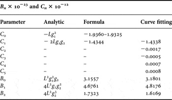
Based on the analytic formula, the representation of negative capacitor with more parameters as degrees of freedom is shown as:
 $$\eqalign{C\left( {v_1,\displaystyle{{dv_1} \over {dt}}} \right) & = C_0 + C_1v_1 + C_2v_1^2 + C_3v_1^3 + C_4v_1^4 \cr & + C_5v_1^5 + \left[ {B_0 + B_1v_1 + B_2v_1^2} \right]\displaystyle{{dv_1} \over {dt}}.}$$
By applying least square method (LSM) to curve fitting the function (39), the parameters of model were obtained as shown in Table 4, that have a good agreement with analytic coefficients of model.
Parameters of nonlinear model of negative capacitor.

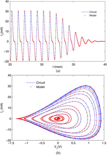
Based on simulation results (V p = 3 V, f c = 1 GHz), the C-V diagram is obtained and the coefficients of model are calculated. In Fig. 10, the simulation results of NIC circuits and negative capacitor model are compared and have a good agreement.
Simulation results of circuit and model of negative capacitance (V p = 3 V, f c = 1 GHz), (a) I 1(t), (b) I 1(t) versus V 1(t).

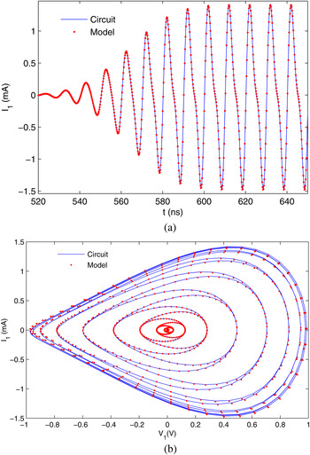
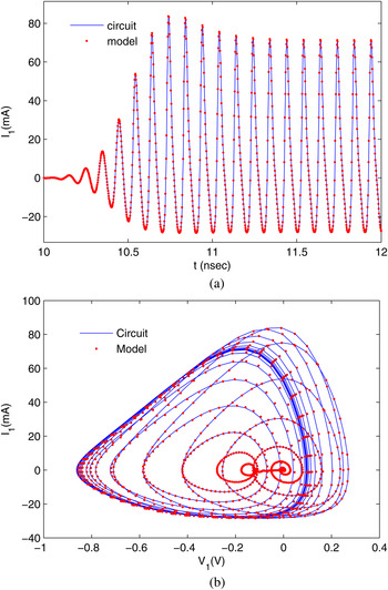
In Fig. 11 (V p = 1 V, f c = 100 MHz) and Fig. 12 (V p = 10 V, f c = 10 GHz), the results of model and circuit simulation are compared in other frequencies to validate model behavior.
Simulation results of circuit and model of negative capacitance (V p = 1 V, f c = 100 MHz), (a) I 1(t), (b) I 1(t) versus V 1(t).

Simulation results of circuit and model of negative capacitance (V p = 10 V, f c = 10 GHz), (a) I 1(t), (b) I 1(t) versus V 1(t).

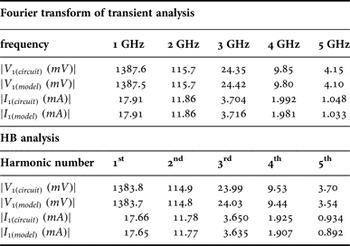
For extra validation of proposed model, the HB analysis of circuit and model are studied. The values of all harmonics are compared with Fourier transform of steady state response of transient analysis in each harmonic frequency. The results are shown for (V p = 3 V, f c = 1 GHz) in Table 5.
Comparsion of the results of the HB and the transient analysis for input signal with V p = 3 V and f c = 1 GHz.

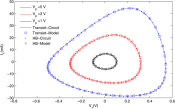
By applying inverse Fourier transform, the time domain response of circuit are calculated from HB results. These results are compared with steady state response of sinusoidal input signal in transient analysis. The V-I steady state cycles for sinusoidal input signal for transient and HB analysis are shown in Fig. 13. The simulations are performed for diffrent amplitudes of input signal in f c = 5 GHz. These results show very good agreements with each other, that validated proposed nonlinear model of negative capacitor.
Simulation results of transient and HB analysis of circuit and proposed model of negative capacitance for various amplitudes of input signal (V p = 1, 3, 5 V) at f c = 5 GHz.

The total capacitance and the time constant of the circuit will be negative and the circuit becomes unstable if the capacitor at the input of circuit is not large enough. By extraction and modeling of negative capacitance in the nonlinear regime and choosing suitable input capacitor and other parameters, the circuit stability can be obtained.
VII. CONCLUSION
Nonlinear analysis of non-Foster structures can be an important step for applying them in circuits with high power level such as power amplifiers and electrically small antennas in the transmitting mode. The analysis in the time domain and the transient response of the circuit helps us to study the stability of circuit and it can be analyzed by using the extracted nonlinear negative capacitor. At the first step, a simple nonlinear model for the transistor was used to analyze these structures. Then by adding parasitic elements to the model, more accurate analysis of the circuit will be presented.
 Hamed Khoshniyat was born in Karaj, Iran, in 1985. He received B.Sc. and M.Sc. degrees from the Amirkabir University of Technology (Tehran Polytechnic), Tehran, Iran, both in Electrical Engineering, in 2008 and 2010 respectively. He is currently working toward Ph.D. degree in “fields and waves” and a Research Assistant in the Wave Propagation and Microwave Measurement Laboratory (WPMML) in electrical engineering at Amirkabir University of Technology (Tehran Polytechnic). His current research interests include analysis and modeling of distributed amplifiers and switches,non-Foster elements, active and passive microwave device and circuits and microwave measurement.
 Abdolali Abdipour was born in Alashtar, Iran, in 1966. He received his B.Sc. degree in Electrical Engineering from Tehran University, Tehran, Iran, in 1989, his M.Sc. degree in Electronics from Limoges University, Limoges, France, in 1992, and his Ph.D. degree in Electronic Engineering from Paris XI University, Paris, France, in 1996. He is currently a professor with the Electrical Engineering Department, Amirkabir University of Technology (Tehran Polytechnic), Tehran, Iran. He has authored five books and has authored or coauthored over 300 papers in refereed journals and local and international conferences. His research areas include wireless communication systems (RF technology and transceivers), RF/microwave/millimeter-wave/THz circuit and system design, electromagnetic (EM) modeling of active devices and circuits, high-frequency electronics (signal and noise), nonlinear modeling, and analysis of microwave devices and circuits.
 Gholamreza Moradi was born in Shahriar, Iran in 1966. He received his B.Sc. in Electrical Communication Engineering from Tehran University, Tehran, Iran in 1989, and the M.Sc. in the same field from Iran University of Science and Technology in 1993. Then he received his Ph.D. degree in Electrical Engineering from Tehran Polytechnic University, Tehran, Iran in 2002. His research areas include applied and numerical Electromagnetics, Microwave measurement, and antenna. He has published more than 50 journal papers and has authored/coauthored five books in his major. He is an associate professor with the electrical engineering department, Amirkabir University of Technology (Tehran Polytechnic), Tehran, Iran. He is now working in Dr. Pedram Mousavi’s research group as a visiting professor at the University of Alberta in Edmonton, Canada.