





1. Introduction
Turbulent boundary layers (TBLs) subjected to adverse pressure gradients (APGs) are relevant to a variety of engineering applications, such as the flows over airfoils or within diffusers. The relevant properties of these APG TBLs are governed by specific flow conditions, namely the local friction Reynolds number, the local streamwise pressure gradient (PG) and the history of streamwise PGs experienced by the TBL upstream of the measurement location (Devenport & Lowe Reference Devenport and Lowe2022). The local friction Reynolds number,
 $Re_{\tau }=\delta {U_{\tau }}/\nu$
, is a fundamental parameter of the TBL which describes the properties of well-behaved, smooth-wall, zero-pressure-gradient (ZPG) TBLs (i.e. canonical TBLs (Marusic et al. Reference Marusic, Chauhan, Kulandaivelu and Hutchins2015; Sanmiguel Vila et al. Reference Sanmiguel Vila, Vinuesa, Discetti, Ianiro, Schlatter and Örlü2017)). Here,
 $\delta$
denotes the boundary-layer thickness (Lozier et al. Reference Lozier, Deshpande, Zarei, Lindić, Rowin and Marusic2025),
 $U_{\tau }$
is the mean friction velocity and
 $\nu$
is the kinematic viscosity. Local streamwise PGs will be quantified in this study using Clauser’s pressure-gradient parameter,
 $\beta =(\delta ^{*}/\rho U_{\tau }^{2})({\rm d}P/\text{d}x)$
, where
 $\delta ^{*}$
is the displacement thickness,
 $\rho$
is the density and
 ${\rm d}P/\text{d}x$
is the local streamwise PG, and
 $x$
and
 $z$
denote the streamwise and wall-normal directions, respectively. Additionally, local PGs are commonly accompanied by varying upstream flow conditions, leading to coupled PG-history effects. While the influences of the local flow conditions (i.e.
 $Re_{\tau }$
and
 $\beta$
) on APG TBL properties, like the mean turbulence statistics, have been studied over many decades (Clauser Reference Clauser1954), fewer studies have sought to systematically decouple and quantify the additional influence of PG history. For instance, it is well established that local streamwise PGs influence the magnitude of turbulent stresses (e.g. the emergence of secondary peaks in the wake region (Skåre & Krogstad Reference Skåre and Krogstad1994; Marusic & Perry Reference Marusic and Perry1995; Deshpande & Vinuesa Reference Deshpande and Vinuesa2024)) and the mean streamwise velocity (e.g. increase in the wake factor,
 $\varPi$
, with
 $\beta$
(Monty et al. Reference Monty, Harun and Marusic2011)). However, a number of recent studies (Devenport & Lowe Reference Devenport and Lowe2022) have demonstrated that PG histories can influence these same turbulence statistics, on par with the influence of local PGs, motivating the need for further studies to decouple these effects.
In particular, the coupled influences of these flow parameters have historically made it difficult to rigorously characterise the sole influence of local APGs on the classical scaling laws for TBL statistics (Nagib & Chauhan Reference Nagib and Chauhan2008; Monty et al. Reference Monty, Harun and Marusic2011; Pozuelo et al. Reference Pozuelo, Li, Schlatter and Vinuesa2022). An example is the classical logarithmic law, which describes the mean velocity profile in the overlap region of the TBL, and is given by
 \begin{align} U^{+} = \frac {1}{\kappa } \ln (z^{+}) + B, \end{align}
where
 $\kappa$
and
 $B$
are the von Kármán and the additive coefficients, respectively. Despite the widespread acceptance of this logarithmic scaling behaviour in the overlap region of high-
 $Re_{\tau }$
canonical TBLs (Smits et al. Reference Smits, McKeon and Marusic2011; Marusic et al. Reference Marusic, Monty, Hultmark and Smits2013), there remain unresolved questions about if, and how,
 $\kappa$
and
 $B$
are influenced by local APGs and PG history individually (Nickels Reference Nickels2004; Nagib & Chauhan Reference Nagib and Chauhan2008; Knopp et al. Reference Knopp, Reuther, Novara, Schanz, Schülein, Schröder and Kähler2021). Consequently, the aim of the present study is to systematically decouple the influences of local APGs and PG history to determine unambiguously how local APGs influence these classical log-law coefficients. In this study,
 $\kappa = 0.39$
and
 $B = 4.3$
will be used for canonical TBLs (Marusic et al. Reference Marusic, Chauhan, Kulandaivelu and Hutchins2015), and the ‘+’ superscript will be used to denote normalisation by viscous velocity (
 $U_{\tau }$
), length (
 $\nu /{U_{\tau }}$
) and/or time (
 $\nu /{U_{\tau }}^2$
) scales.
1.1. Investigation of the classical logarithmic-law coefficients
There are a number of considerations, outlined here, that help ensure investigations of the classical log-law in APG TBLs are rigorous and systematic. First, the classical scaling laws for mean TBL statistics are observed at sufficiently high Reynolds numbers, where a clear separation exists between the inner and wake regions of the TBL, and where the extent of the overlap region permits unambiguous evaluation of these laws (Smits et al. Reference Smits, McKeon and Marusic2011). Here, we consider the high-
 $Re_{\tau }$
regime to correspond to
 $Re_{\tau } \gtrsim 4500$
, consistent with Marusic et al. (Reference Marusic, Monty, Hultmark and Smits2013), as shown in figure 1(a). Along similar lines, strong local PGs (
 $\beta \gtrsim O(10)$
; see figure 1
a) have also been found to influence the extent of the overlap region. Specifically, increasing local APG strength corresponds to a decrease in the upper limit of the overlap region (Marusic & Perry Reference Marusic and Perry1995; Knopp et al. Reference Knopp, Reuther, Novara, Schanz, Schülein, Schröder and Kähler2021). While many studies have examined low-
 $Re_{\tau }$
TBLs and/or TBLs subjected to strong APGs (e.g. leading to separation), which are relevant to many applications, such conditions are not well suited for evaluating the log-law. The combination of limited scale separation and/or strong local APG effects can significantly compress (or obscure) the overlap region, thereby introducing uncertainty in reported variations of
 $\kappa$
and/or
 $B$
. Another consideration, particularly for PG TBLs, is the influence of PG history. For example, changes in
 $B$
have previously been linked to both
 $\beta$
(Nagano et al. Reference Nagano, Tsuji and Houra1998; Monty et al. Reference Monty, Harun and Marusic2011) and PG-history effects (Bobke et al. Reference Bobke, Vinuesa, Örlü and Schlatter2017; Gungor et al. Reference Gungor, Gungor and Maciel2024; Preskett et al. Reference Preskett, Virgilio, Jaiswal and Ganapathisubramani2025). Because real-life applications almost always involve sources of PG history (e.g. airfoil geometries), many studies have been designed to introduce targeted PG-history effects at both low and high
 $Re_{\tau }$
(Bobke et al. Reference Bobke, Vinuesa, Örlü and Schlatter2017; Gungor et al. Reference Gungor, Gungor and Maciel2024; Preskett et al. Reference Preskett, Virgilio, Jaiswal and Ganapathisubramani2025). In such cases,
 $\kappa$
and
 $B$
may be influenced by both
 $\beta$
and the imposed PG histories, which are unique to each study. Decoupling these influences, in order to isolate the effects of either
 $\beta$
or PG history alone, requires additional cases and measurements with systematic, well-controlled variations in PG history and local flow conditions.
(a) The
 $\beta (Re_{\tau })$
map of a selection of APG TBLs datasets from the literature, including numerical and experimental studies. The yellow-shaded area represents the region of interest for the present study, i.e. high
 $Re_{\tau }$
and low-to-moderate
 $\beta$
where a well-defined overlap region is expected. (b) Schematic representation of the different regions of TBL development typically encountered in high-
 $Re_{\tau }$
APG experiments. (c) Comparison of experimental parameters between the present study and those reported by Knopp et al. (Reference Knopp, Reuther, Novara, Schanz, Schülein, Schröder and Kähler2021) and Romero et al. (Reference Romero, Zimmerman, Philip, White and Klewicki2022).
 $\delta _{\textit{ref}}=\delta (x=x_{\textit{ref}})$
.

Figure 1. Long description
Panel A: A scatter plot showing the relationship between the friction Reynolds number (Reτ) and the pressure-gradient parameter (β). The x-axis represents Reτ, ranging from 10^2 to 10^4, and the y-axis represents β, ranging from 10^-2 to 10^2. Different symbols and colors represent data from various studies. A yellow-shaded region indicates the area of interest for the present study. Panel B: A line graph illustrating the different regions of turbulent boundary layer (TBL) development. The x-axis represents the streamwise direction (x) normalized by a reference length (xref), and the y-axis represents the pressure coefficient (Cp). The graph shows regions of upstream perturbations, zero pressure gradient (ZPG), and adverse pressure gradient (APG). Panel C: A comparison of experimental parameters among the present study and two other studies. The x-axes represent different normalized parameters (|dCp/dx|, xrelax/deref, and xdevelop/deref), and the y-axis shows the corresponding values. Different symbols represent data from the present study and the other studies.
To highlight the significance of the experimental dataset evaluated in the present study, we compare the corresponding parametric space with that of previous investigations. The
 $\beta (Re_{\tau })$
mappings for a selection of previous APG TBL datasets are presented in figure 1(a) for reference. This figure illustrates the wide range of
 $Re_{\tau }$
,
 $\beta$
and PG history conditions that have already been investigated, both numerically and experimentally. However, in the parameter space best suited to investigate the log-law coefficients (i.e. the region of high
 $Re_{\tau }$
and low-to-moderate
 $\beta$
highlighted in yellow in figure 1
a) only a limited number of experimental studies have investigated the scaling of APG TBL statistics (at least in part). Additionally, the APG conditions in past experiments have all been generated using different methods, namely adjustable converging and/or diverging ceilings (Sanmiguel Vila et al. Reference Sanmiguel Vila, Vinuesa, Discetti, Ianiro, Schlatter and Örlü2020; Volino Reference Volino2020; Parthasarathy & Saxton-Fox Reference Parthasarathy and Saxton-Fox2023), ramp structures (Knopp et al. Reference Knopp, Reuther, Novara, Schanz, Schülein, Schröder and Kähler2021; Romero et al. Reference Romero, Zimmerman, Philip, White and Klewicki2022) or wall-normal transpiration (Clauser Reference Clauser1954; Deshpande et al. Reference Deshpande, Van Den Bogaard, Vinuesa, Lindić and Marusic2023). A generalised schematic of the streamwise PG variations, which are representative of these past APG TBL experiments, is shown in figure 1(b). In general, the most upstream region often experiences favourable-PG conditions, introduced by the geometry of the ramp or ceiling (see for instance Sanmiguel Vila et al. Reference Sanmiguel Vila, Vinuesa, Discetti, Ianiro, Schlatter and Örlü2020; Knopp et al. Reference Knopp, Reuther, Novara, Schanz, Schülein, Schröder and Kähler2021; Romero et al. Reference Romero, Zimmerman, Philip, White and Klewicki2022). Although these upstream PG conditions are highly set-up/facility-dependent, any non-zero PGs in the farthest upstream region are referred to, and interpreted, here as ‘perturbations’, because they can potentially influence the downstream development of the TBL. These upstream PG perturbations are typically followed by a nominally ZPG ‘relaxation’ region, designed to damp the effects of these perturbations and re-establish a canonical TBL state. The APG conditions are then introduced farther downstream in a ‘development’ region where the APG TBLs are typically measured. While most experimental designs include a relatively long relaxation region, to minimise upstream PG-history effects and ensure a well-defined baseline prior to the onset of APG conditions, each experimental configuration is associated with a distinct PG history. This variability/uniqueness of each set-up complicates direct comparisons between different APG TBL datasets, as it is uncertain if the turbulence statistics in the development region retain any influences from the specific PG histories imposed upstream. This also underscores the benefit of investigating APG TBLs with minimal upstream history effects.
Additionally, quantifying these unique PG histories empirically remains an active topic of investigation (Vinuesa et al. Reference Vinuesa, Örlü, Sanmiguel Vila, Ianiro, Discetti and Schlatter2017; Gomez & McKeon Reference Gomez and McKeon2025; Mahajan et al. Reference Mahajan, Deshpande, Gungor, Maciel and Vinuesa2025; Virgilio et al. Reference Virgilio, Preskett, Jaiswal and Ganapathisubramani2025). However, PG histories are (broadly) described by the variations in
 $\beta (Re)$
, or
 $\beta (x)$
, observed upstream of a measurement location (e.g. the accumulation of, and/or the rate of change of,
 $\beta$
). The present experimental approach does not permit quantification of
 $\beta (Re_{\tau })$
or
 $\beta (x)$
with sufficient streamwise resolution; instead, we measure streamwise profiles of the pressure coefficient,
 \begin{align} C_{\!P}(x)=1- \frac {U_{\infty }^{2}(x)}{U_{\infty }^{2}(0)}, \end{align}
where
 $U_{\infty }(x)$
is the free stream velocity and
 $x=0$
denotes the wind tunnel test section inlet. The PG history can then be expressed as
 $\beta (x) = ({\delta ^{*}}/{C_{\!f})} ({\text{d}C_{\!P}}/{\text{d}x}) (1-C_{\!P})^{-1}$
, where
 $C_{\!f}$
is the local friction coefficient. For most APG TBLs (especially the high-Reynolds-number low-to-moderate APG TBLs which are relevant to this study),
 $({\delta ^{*}}/{C_{\!f}})$
and
 $Re_{\tau }$
are expected to increase monotonically with
 $x$
. As such, in the present study, any differences in
 $C_{\!P}(x)$
upstream of a given measurement location would result in (qualitative) differences in streamwise PG history (figure 1
b). It is also noted here that other upstream perturbations, such as discrete changes in wall-roughness or tripping conditions, also influence TBL development and are generally classified as history effects (Hanson & Ganapathisubramani Reference Hanson and Ganapathisubramani2016); however, the present study maintains hydrodynamically smooth walls and matched tripping conditions across all cases. Accordingly, the discussion of history effects in this study is limited exclusively to differences in streamwise PG history. Further, the discussion of streamwise PG histories here will consider the implications of both the PG conditions experienced by the TBL immediately upstream of the measurement location, and the PG conditions experienced by the TBL, cumulatively, between the inlet and the measurement location.
1.2. Present approach
Figure 1(a) also highlights a gap in the literature concerning the investigation of high-Reynolds-number TBLs under low-to-moderate APGs. Although datasets such as Romero et al. (Reference Romero, Zimmerman, Philip, White and Klewicki2022) cover a part of this parameter space, the influence of their unique PG history (due to a ramp structure) remains unquantified and coupled with the influence of the local APG. The present study addresses this gap by leveraging a unique large-scale experimental facility (Marusic et al. Reference Marusic, Chauhan, Kulandaivelu and Hutchins2015; Deshpande et al. Reference Deshpande, Van Den Bogaard, Vinuesa, Lindić and Marusic2023), and a systematic methodology, to generate high-
 $Re_{\tau }$
moderate-APG TBLs with well-controlled upstream PG histories (figure 2), consistent with the conceptual framework illustrated in figure 1.
First, this methodology is used to produce TBLs with matched
 $Re_{\tau }$
and
 $\beta$
downstream, but with distinct upstream PG histories. This approach enables decoupling of the influences of PG history and the local flow conditions on APG TBL development. In contrast to previous experiments, this methodology facilitates a controlled and systematic investigation of PG-history effects, characterised by relatively weak upstream PG perturbations (low
 $|\text{d}C_{\!P}/\text{d}x|$
), extended relaxation and development regions (as shown in figure 1
c), and well-matched/controlled local flow conditions downstream. The premise underlying this approach is that if differences in APG TBL statistics are detectable under weakly varying PG histories, it is reasonable to expect that similar effects will persist, and potentially strengthen, under stronger PG perturbations and/or shorter relaxation and development distances. As such, this systematic analysis enables more conclusive insights into the scaling of APG TBL statistics within the parameter space described above, which are also qualitatively relevant to other experiments, although we do not aim to directly extrapolate these quantitative effects to other parameter spaces. Additionally, the present comparisons between APG TBLs with different PG histories will provide insight into outstanding questions, such as the relaxation and development lengths required to damp upstream PG perturbations in high-
 $Re_{\tau }$
experiments, the extent to which different regions of the TBL are influenced by PG history, and related effects.
Finally, the same methodology will be applied to generate high-
 $Re_{\tau }$
TBLs with varying low-to-moderate local APGs over an extended downstream fetch, while prescribing strictly controlled ZPG conditions in the upstream region, to minimise PG-history effects, addressing limitations of previous studies. The high-
 $Re_{\tau }$
conditions, low-to-moderate APGs and minimal PG history achieved here ensure a sufficiently broad overlap region extent to unambiguously investigate the influence of local APGs on the classical log-law. For this purpose, we will also incorporate oil-film interferometry (OFI) to obtain independent friction velocity measurements, which are crucial for the investigation of normalised turbulence statistics. These results will also form the basis for Part 2, where new physical insights into the roles of
 $Re_{\tau }$
, local APGs and PG history in TBL statistics will be combined with the framework of Nickels (Reference Nickels2004) and a broad range of APG TBL datasets available in the literature to reconstruct a robust composite profile for the mean streamwise velocity.
(a) Schematic of the experimental set-up established in Deshpande et al. (Reference Deshpande, Van Den Bogaard, Vinuesa, Lindić and Marusic2023), to generate high-
 $Re_{\tau }$
APG TBLs with controlled upstream pressure-gradient histories. Conceptual profile of
 $C_{\!P}(x)$
along the test section to investigate a ZPG and APG TBLs with (b) minimal PG history or (c) with a controlled upstream PG perturbation, following the framework of figure 1(b).

2. Experimental set-up and methodology
Experiments were conducted in the high-Reynolds-number boundary layer wind tunnel at the University of Melbourne. The test section has a cross-sectional area of
 $1.89 \times 0.92\,{\textrm {m}}^{2}$
and a working length of 27 m (figure 2
a), enabling the development of physically thick TBLs with high friction Reynolds numbers towards the downstream end. Inlet flow conditioning ensures that free stream turbulence intensities remain below 0.4 % throughout the test section. The test section ceiling is equipped with an array of adjustable air-bleed slots spanning the full width, distributed quasiperiodically in the streamwise direction. These slots permit controlled bleeding of air from the test section, driven by the internal static pressure which is regulated by altering the blockage at the test section outlet. For example, a nominal ZPG TBL is obtained by installing a single high-porosity mesh at the outlet and keeping all air-bleed slots fully open. A detailed characterisation of this set-up for ZPG TBLs is provided by Marusic et al. (Reference Marusic, Chauhan, Kulandaivelu and Hutchins2015). Following Deshpande et al. (Reference Deshpande, Van Den Bogaard, Vinuesa, Lindić and Marusic2023), the test section static pressure can be increased by installing one or more low-porosity (higher-blockage) screens at the outlet. This produces nominally APG conditions where the air-bleed slots are open, and ZPG conditions where they are restricted or closed (figures 2
b and 2
c). This approach enables the generation of well-controlled APG TBLs, representative of practical conditions, with minimal physical modifications to the test section. Figures 2(b) and 2(c) also illustrate how different PG histories, i.e. streamwise variations in the pressure coefficient, can be achieved by selectively opening and/or closing these air-bleed slots.
The
 $C_{\!P}(x)$
profiles measured for the (a) ZPG, Ref. APG3 and Perturbed cases, and the (b) ZPG, APG1 and APG3 cases (see table 1 for exact flow conditions). Vertical dashed lines indicate the locations of streamwise velocity and OFI measurements. Here
 $\delta _1$
denotes the value of
 $\delta$
at
 $x_1$
for the ZPG case. In the APG regions,
 $\text{d}C_{\!P}/\text{d}x$
is nominally 0.025 for the APG3 and Perturbed cases and 0.015 for the APG1 case.

2.1. Imposing controlled pressure-gradient histories
Figure 3 presents the experimentally measured pressure coefficient profiles,
 $C_{\!P}(x)$
, for various test section configurations, as listed in table 1. For each configuration, the free stream dynamic pressure was measured along the streamwise extent of the test section using a Pitot–static tube mounted at
 $z = 0.525$
m on the streamwise traverse system (figure 2
a). The most basic configuration corresponds to nominal ZPG conditions throughout the test section, indicated by black symbols in figure 3. Across all ZPG cases tested, variations in
 $U_{\infty }$
remained within 1 % along the entire test section fetch (
 $C_{\!P}(x)=0\pm 0.012$
). In figure 3 and table 1, square and circle symbols denote inlet unit Reynolds numbers of
 $ U_{\infty }(x=0)/\nu \approx 9 \times 10^5\ \mathrm{m}^{-1}$
and
 $ 6 \times 10^5\ \mathrm{m}^{-1}$
, respectively. To generate different APG configurations, either one or three low-porosity screens were added to the outlet, in addition to the high-porosity mesh. These are denoted as APG1 (green symbols in figure 3
b) and APG3 (red symbols in figures 3
a and 3
b). As shown in figure 3(b), both the APG1 and APG3 configurations exhibit nominal ZPG conditions upstream of the APG development region (
 $ x \lt 9\ \mathrm{m}$
), consistent with the set-up illustrated in figure 2(b). These cases are referred to as having minimal upstream PG history and serve as the reference cases for comparison with those with selectively imposed PG histories. The TBL statistics for the APG1 and APG3 cases were found to collapse with those from the ZPG case at
 $ x = 8.5\ \mathrm{m}$
, confirming the absence of significant PG-history effects upstream of this location, consistent with the findings of Deshpande et al. (Reference Deshpande, Van Den Bogaard, Vinuesa, Lindić and Marusic2023). An additional configuration, referred to as the Perturbed case, was then designed to introduce a controlled PG history which was distinct from the baseline APG cases. Specifically, this set-up modifies the pattern of open/closed air-bleed slots in the upstream region, relative to the APG3 case (figures 2
b and 2
c). The resulting
 $ C_{\!P}(x)$
profile is shown by blue symbols in figure 3(a). For this case, the inlet and downstream flow conditions were matched to the APG3 reference configuration (Ref. APG3), but notable differences in
 $ C_{\!P}(x)$
appear for
 $x \lt 12\ \mathrm{m}$
due to the imposed PG perturbation (i.e. APG conditions for
 $x\lt 5$
m). The Perturbed case was also designed to include a long relaxation region (i.e. nominally ZPG conditions for
 $ 5 \lt x \lt 12\ \mathrm{m}$
) following the initial PG perturbation, enabling assessment of how the initial upstream PG perturbation modifies the TBL development compared with the reference cases. Farther downstream, the facility permits sustained APG development, over a long streamwise distance, enabling a detailed comparison of the differences in development between the Perturbed and Ref. APG3 cases under locally matched flow conditions (
 $ x \gt 12\ \mathrm{m}$
). Appendix B contains additional details about the exact configurations of open and closed slats required to generate the Perturbed and Ref. APG3 cases.
Characteristics of the experimental TBLs investigated in the present study.

Table 1. Long description
The table presents data for different cases, including ZPG, Ref. APG3, Perturbed, APG1, and APG3. It includes measurements such as x (m), beta, Re_tau, Re_theta, u_tau, delta_99 (mm), delta (mm), and theta* (mm). The table is divided into two main sections: from figure 3(a) and from figure 3(b). Each section lists specific cases with their corresponding values. For example, in the first section, the ZPG case at x = 5.1 m has Re_tau of 4090 and Re_theta of 8970, while the Perturbed case at the same x has Re_tau of 4060 and Re_theta of 9550. The table also includes symbols representing each case.
2.2. Streamwise velocity and friction velocity measurements
Five measurement stations were chosen, spanning a significant streamwise fetch, where both the streamwise turbulence statistics and friction velocity could be measured reliably. Specifically, the stations
 $x_a$
and
 $x_1$
were chosen because they are expected to exhibit the highest contrast in turbulence statistics between the Perturbed and reference cases (due to their relative proximities to changes in PG conditions, figure 3
a). The stations
 $x_b$
,
 $x_c$
and
 $x_2$
are then used to assess the longer-scale recovery of the Perturbed case, towards the reference cases, under sustained matched flow conditions. However, it is noted that the physical transitions from one PG condition to another do not occur as distinct, step-like changes. This makes the determination of the exact streamwise location where a new PG condition is established difficult, and the above distances are considered conservative estimates (see Appendix B). In the relaxation region,
 $x_a$
 $x_b$
and
 $x_c$
are located approximately 2, 27 and 50
 $\delta _{a}$
downstream of the establishment of ZPG conditions in the Perturbed case, respectively, where
 $\delta _{a}$
is the boundary-layer thickness at
 $x_a$
. Similarly, in the development region,
 $x_1$
and
 $x_2$
are located approximately 2 and 17
 $\delta _{1}$
downstream of the re-establishment of APG conditions in the Perturbed case, respectively, where
 $\delta _{1}$
is the boundary-layer thickness at
 $x_1$
. In contrast,
 $x_1$
and
 $x_2$
are located approximately 11 and 26
 $\delta _{1}$
downstream of the establishment of APG conditions in the Ref. APG3 case, respectively. The mentioned development lengths are approximate, since the PG transition can only be located within the streamwise resolution of the
 $C_{\!P}(x)$
measurements. With a minimum spacing of
 $0.5$
m between adjacent pressure measurements, the corresponding uncertainty is approximately
 $\pm 0.25$
m.
Streamwise velocities were measured at several wall-normal locations using a single hot-wire made in-house from Wollaston wire mounted on a Dantec 55P15 probe. The wire was etched to a sensing diameter
 $ d = 2.5\,{\unicode[Arial]{x03BC}} \mathrm{m}$
with fixed aspect ratio
 $ l/d = 200$
, giving a nominal length
 $ l = 0.5\,\mathrm{mm}$
and resulting viscous-scaled lengths
 $ l^+ = 11{-}16$
across all cases. To resolve the energetic hierarchy of scales in the TBL, the sampling time
 $ T_S$
was chosen to satisfy
 $ T_S U_{\infty }/\delta \ge 20\,000$
. The sampling frequency was fixed at 50 kHz, and the signal was low-pass filtered at 25 kHz. The resulting viscous-scaled sampling intervals
 $ t_S^+ = {U_{\tau }}^2 /(f_S \nu )$
ranged from 0.08 to 0.31, sufficient to resolve the relevant small-scale motions. Further details of the experimental apparatus and calibration methods are available in Deshpande et al. (Reference Deshpande, Van Den Bogaard, Vinuesa, Lindić and Marusic2023). OFI was used at each streamwise measurement location (except
 $x=x_c$
) to obtain an accurate and independent estimate of
 $ {U_{\tau }}$
. Further details of the OFI methodology implemented in the present APG TBL experiments are provided in Marusic et al. (Reference Marusic, Abu Rowin, Lozier, Lindić, Zarei and Deshpande2025). Taking into account uncertainties associated with oil viscosity calibration, interference pattern resolution and potential contamination of the oil droplets, the estimated uncertainty in the measured friction velocity was approximately
 $\pm 1$
%.
2.3. Summary of present experimental dataset
Key characteristics for the TBLs investigated here, obtained from these hot-wire, OFI and
 $C_{\!P}$
measurements at each measurement location, along with their respective symbols, are presented in table 1. The recent approach of Lozier et al. (Reference Lozier, Deshpande, Zarei, Lindić, Rowin and Marusic2025) was employed to determine the TBL thickness,
 $\delta$
, which is compared with the classical
 $\delta _{99}$
, estimated using the method of Vinuesa et al. (Reference Vinuesa, Bobke, Örlü and Schlatter2016), in table 1. The capability of the present methodology for creating controlled PG histories can now be demonstrated quantitatively using the characteristics tabulated in table 1. First, for the cases in figure 3(a),
 $Re_{\tau }(x)$
is measured to be nominally matched between the Perturbed and ZPG cases in the upstream section (
 $x \lt 12$
m). This is an important condition for investigating the persistence of any PG-history effects observed within the relaxation region that may result from the upstream APG perturbation. In the downstream section (
 $x \gt 12$
m) where
 $C_{\!P}$
and
 $\text{d}C_{\!P}/\text{d}x$
are matched for the Perturbed and Ref. APG3 cases (figure 3
a),
 $Re_{\tau }(x)$
and
 $\beta (x)$
are also confirmed to be nominally matched (table 1). This is the critical condition for decoupling the local and upstream PG effects (Bobke et al. Reference Bobke, Vinuesa, Örlü and Schlatter2017; Mahajan et al. Reference Mahajan, Deshpande, Gungor, Maciel and Vinuesa2025), and quantifying the influence of upstream PG perturbations on the APG TBL development in the downstream development region. Finally, in figure 3(b), although the local PG (i.e.
 $\beta$
) varies, the Reynolds number is found to be nearly identical between the ZPG, APG1 and APG3 cases with matched inlet conditions, as shown in table 1. This ensures that the effects of the local APG on the TBL statistics and scaling laws can be rigorously evaluated without the additional influence of varying Reynolds numbers and/or PG-history effects.
3. PG-history effects in high-Reynolds-number APG TBLs
3.1. Streamwise mean velocity
We first examine viscous-scaled mean streamwise velocity profiles (
 $U^{+}$
) measured in the relaxation region, i.e. at
 $x_a$
,
 $x_b$
and
 $x_c$
(figure 3
a), which are shown in figure 4(a). The ZPG case is used here as a reference. Although the flow conditions for the Perturbed case are locally matched to the ZPG case in the relaxation region (table 1), differences in their mean velocity profiles can be seen at
 $x_a$
attributed to the upstream APG perturbation experienced by the Perturbed case (figure 3
a). Specifically, the Perturbed mean velocity profile (
 $U^{+}$
) in the wake region lies above the ZPG profile, and the Perturbed profile in the overlap region is slightly below the ZPG profile at
 $x_a$
(figure 3
a). This is made clearer by subtracting the classical log-law (1.1) from these measured mean velocity profiles (
 $U^{+}-U^{+}_{log}$
), which reveals a systematic deviation from this canonical scaling behaviour in the Perturbed profile, figure 4(b). It is also noted that the mean velocity profile in the inner region remains largely unaffected by the upstream APG perturbation, consistent with the findings of Bobke et al. (Reference Bobke, Vinuesa, Örlü and Schlatter2017) and Pozuelo et al. (Reference Pozuelo, Li, Schlatter and Vinuesa2022).
(a) Profiles of mean streamwise velocity, and (b) deviations from the classical log-law for the ZPG and Perturbed cases in the relaxation region. Both cases have locally matched flow conditions. The inset in (b) shows the profile at
 $x=x_a$
. Note the profiles for
 $x=x_b$
and
 $x=x_c$
are vertically offset.

Figure 4. Long description
Panel A: A line graph shows profiles of mean streamwise velocity (U+) against the dimensionless wall-normal coordinate (z+). The graph includes data for ZPG (gray squares) and Perturbed cases (blue squares) with three different profiles labeled as x_a, x_b, and x_c. The lines represent different theoretical models: U+ = z+ (dotted line) and U+ = (1/κ)ln(z+) + B (dashed line). Panel B: Another line graph depicts deviations from the classical log-law for the ZPG and Perturbed cases in the relaxation region. The y-axis represents U+ - (1/κ)ln(z+) - B, and the x-axis is the dimensionless wall-normal coordinate (z+). The inset shows a zoomed-in view of the profile at z+ = 100. The Perturbed case data (blue squares) are vertically offset for clarity.
(a,b) Profiles of mean streamwise velocity, (c,d) indicator function and (e,f) deviations from the classical log-law for the ZPG, Ref. APG3 and Perturbed cases in the development region at (a,c,e)
 $x=x_1$
and (b,d,f)
 $x=x_2$
. All APG cases have locally matched local flow conditions, but unique PG histories. The ZPG cases have locally matched
 $Re_{\tau }$
.

Farther downstream, the Perturbed mean velocity profiles collapse with the reference ZPG profiles at
 $x_b$
and
 $x_c$
(figure 4
a). This collapse is further confirmed by figure 4(b), where both cases show good agreement with the classical log-law. However, differences in characteristics such as the TBL thickness (
 $\delta$
, see table 1), and its growth rate (
 $\text{d}\delta /\text{d}x$
), still persist as a result of the upstream APG perturbation. For example, across the full relaxation region (i.e. between
 $x_a$
and
 $x_c$
where
 $x_c - x_a \approx 48\delta _a$
) the growth rate of the Perturbed TBL is 25 % greater than the reference ZPG TBL. This effect is attributed primarily to the large-scale motions (LSMs), which are energised by the upstream APG perturbation (see figure 6
c), and leads to enhanced momentum transport in the TBL. Both observations are significant: the mean velocity profile does recover ZPG scaling, suggesting that the effect of upstream PG perturbations (like those introduced by ramps) on mean turbulence statistics can be minimised with a sufficiently long relaxation length ((Knopp et al. Reference Knopp, Reuther, Novara, Schanz, Schülein, Schröder and Kähler2021; Romero et al. Reference Romero, Zimmerman, Philip, White and Klewicki2022) see figure 1), however, the boundary-layer thickness and growth rate differ from the reference ZPG case, even after a reasonably long relaxation length, making careful comparisons challenging. These results also motivate further investigation into the quantification of PG-history effects, specifically methods/parameters which can account for the specific differences in behaviour observed between
 $x_a$
and
 $x_b$
(or
 $x_c$
).
The mean velocity profiles measured in the development region, i.e. at
 $x_1$
and
 $x_2$
(figure 3
a), are shown in figures 5(a) and 5(b). Here, the Perturbed and Ref. APG3 cases have nominally matched values of
 $Re_{\tau }$
and
 $\beta$
(table 1), and the ZPG case has a matched
 $Re_{\tau }$
. While the mean velocity profiles near the wall (
 $z^{+}\leq 20$
) appear largely unaffected by either the local or upstream PGs at both
 $x_1$
and
 $x_2$
(Pozuelo et al. Reference Pozuelo, Li, Schlatter and Vinuesa2022), the effect of the local APG (
 $\beta$
) can be observed at
 $x_2$
where the Ref. APG3 and Perturbed profiles collapse and deviate significantly from the ZPG profile in the wake and overlap regions (Monty et al. Reference Monty, Harun and Marusic2011; Deshpande et al. Reference Deshpande, Van Den Bogaard, Vinuesa, Lindić and Marusic2023). However, at
 $x_1$
, the influence of PG history is also apparent; although both the Perturbed and Ref. APG3 profiles deviate from the ZPG case, they do not collapse, consistent with the observations of Bobke et al. (Reference Bobke, Vinuesa, Örlü and Schlatter2017). These differences at
 $x_1$
are attributed to the different upstream PG conditions experienced by the two boundary layers before arriving at the same local conditions (i.e.
 $C_{\!P}(x)$
for
 $x_{b}\lt x\lt x_{1}$
). Specifically, the Perturbed profile falls between the ZPG and Ref. APG3 profiles, reflecting a ‘lag’ in APG development (compared with the Ref. APG3 case which has matched conditions) due its upstream PG history (i.e. transitioning from established ZPG conditions). These results further motivate the development of methods/frameworks for quantifying PG-history effects that can account for the differences in behaviour observed between
 $x_1$
and
 $x_2$
; one such framework, motivated by the above observations, is proposed in Part 2.
The influence of local and upstream PGs on the classical log-law is further investigated by plotting the indicator function (
 $z^{+} {\rm d}U^{+} /{\rm d}z^{+}$
) of each mean velocity profile, as shown in figures 5(c) and 5(d). At both measurement locations, and for all PG cases, a clear plateau is observed in the overlap region (
 $10^2\lesssim z^{+} \lesssim 10^3$
), confirming the existence of logarithmic scaling in this region and a sufficient separation between the inner and wake regions in all cases. Additionally, within experimental uncertainty, no systematic changes are observed in the von Kármán coefficient (
 $\kappa$
) due to either local or upstream PGs. The differences in the mean velocity profiles in the wake region also confirm that the wake parameter (
 $\varPi$
) systematically increases with
 $\beta$
(figure 5
d, Monty et al. (Reference Monty, Harun and Marusic2011)), and PG history (figure 5
c, Bobke et al. (Reference Bobke, Vinuesa, Örlü and Schlatter2017)). Finally, the classical log-law (1.1) was subtracted from the measured mean velocity profiles in figures 5(e) and 5(f), in a manner analogous to figure 4(b). In the overlap region, a systematic and significant decrease in the magnitude of the additive coefficient
 $B$
is observed with increasing
 $\beta$
, especially at
 $x_2$
. However, PG history is also seen to affect the value of
 $B$
at
 $x_1$
, as the Ref. APG3 and Perturbed cases do not collapse in figure 5(e), consistent with the lag in APG development noted earlier. It is also noted that the mean velocity profile of the Perturbed case at
 $x_1$
does not collapse with the ZPG case either, as shown in figure 5(a,c,e) where differences in the wake and overlap regions are beyond experimental uncertainty. This confirms that APG conditions are well-established, and influencing the mean turbulence statistics, by this measurement location (i.e.
 $x_1$
is sufficiently downstream of the region with nominally ZPG conditions).
3.2. Streamwise normal stress and premultiplied energy spectra
We now examine the influence of local and upstream PGs on second-order turbulence statistics and the hierarchy of energetic turbulent motions in the TBL. To this end, it is useful to first contextualise the role of LSM in high-
 $Re_{\tau }$
TBLs (e.g. motions associated with attached-eddies and/or superstructures). These LSMs constitute the primary energy-containing motions in the overlap and wake regions of high-
 $Re_{\tau }$
TBLs, and their contributions become increasingly significant with higher Reynolds numbers (Marusic et al. Reference Marusic, Monty, Hultmark and Smits2013, Reference Marusic, Chauhan, Kulandaivelu and Hutchins2015). In the context of APG flows, it has been established that the magnitude and extent of these LSMs and/or superstructures, in the overlap and wake regions, are influenced by local PGs (Deshpande et al. Reference Deshpande, Van Den Bogaard, Vinuesa, Lindić and Marusic2023). Recent studies (Bobke et al. Reference Bobke, Vinuesa, Örlü and Schlatter2017; Pozuelo et al. Reference Pozuelo, Li, Schlatter and Vinuesa2022) have also demonstrated that upstream PGs can leave a persistent footprint on the LSMs in the wake region of low-Reynolds-number TBLs. Hence, it is important to decouple the influences of these local and upstream PGs on the hierarchy of inertia-dominated turbulent motions. The present high-
 $Re_{\tau }$
experiments are critical to achieve this objective as they offer sufficient separation between the viscous and inertia-dominated regions of the TBL, facilitating detailed examination of these influences.
To investigate the distribution of turbulent energy across different scales, the premultiplied spectra of streamwise velocity fluctuations (
 $f\phi _{uu}^+$
) are plotted as a function of their viscous time scale (
 $T^+={U_{\tau }}^2/ f\nu$
) and wall-normal location (
 $z^{+}$
) in figures 6(c) and 6(d) corresponding to the streamwise locations
 $x_a$
and
 $x_b$
, respectively. The corresponding wall-normal profiles of the streamwise normal stress (
 $\overline {u^{2}}^+$
) are also plotted in figure 6(a). Some differences in the streamwise normal stress profiles (figure 6
a) and premultiplied spectra (figure 6
c) are observed in the overlap and wake regions (
 $z^{+}\gtrsim 100$
) at
 $x_a$
between the ZPG and Perturbed cases, attributed to differences in their respective PG histories upstream of this measurement location (figure 3
a). In figures 6(c) and 6(d), the horizontal dash–dotted lines denote the characteristic, Reynolds-number-dependent time scale associated with LSMs in canonical TBLs. At
 $ x_a$
, a secondary spectral peak appears for the Perturbed case (figure 6
c), aligned with this characteristic time scale, highlighting a persistent influence of the upstream APG perturbation (Deshpande et al. Reference Deshpande, Van Den Bogaard, Vinuesa, Lindić and Marusic2023). This spectral feature also corresponds with elevated wake region turbulence intensities in the Perturbed normal stress profile, and reinforces the conclusion that the upstream PG perturbation leaves a measurable footprint at this location. Farther downstream, however, at
 $ x_b$
, both the normal stress profiles (figure 6
a) and premultiplied spectra (figure 6
d) for the ZPG and Perturbed cases collapse, indicating recovery from the upstream PG perturbation. This collapse is also observed at
 $ x_c$
; however, analysis at that location is omitted here for brevity, citing consistency with the trends noted in the mean velocity profiles.
(a) Profiles of streamwise normal stress (
 $\overline {u^{2}}^+$
) for the ZPG and Perturbed cases in the relaxation region. Premultiplied energy spectra (
 $f\phi _{uu}^+$
) at (c)
 $x=x_a$
and (d)
 $x=x_b$
. Vertical dashed lines indicate
 $z^{+}=0.4Re_{\tau }$
and horizontal dot–dashed lines denote
 $T^+=4.8\delta ^{+}/U_{\infty }^{+}$
. (b) Premultiplied spectra at a single wall-normal location corresponding to the vertical dashed lines in (c) and (d). Note that the profiles for
 $x=x_b$
and
 $x=x_c$
are vertically offset in (a) and (b).

Figure 6. Long description
Panel A: A line graph shows profiles of streamwise normal stress for ZPG and Perturbed cases in the relaxation region. The x-axis represents a dimensionless wall-normal coordinate, and the y-axis represents the dimensionless streamwise normal stress. The graph includes two data series: one for ZPG (gray squares) and one for Perturbed (blue squares). Panel B: A line graph displays premultiplied energy spectra at a single wall-normal location. The x-axis represents a dimensionless frequency, and the y-axis represents the premultiplied energy spectra. Two data series are shown: one for ZPG (gray line) and one for Perturbed (blue line). Panel C: A contour plot shows premultiplied energy spectra at a specific streamwise location for the ZPG and Perturbed cases. The x-axis represents the dimensionless frequency, and the y-axis represents the dimensionless wall-normal coordinate. Contour lines indicate different levels of premultiplied energy spectra. Panel D: Another contour plot shows premultiplied energy spectra at a different streamwise location for the ZPG and Perturbed cases, with similar axes and contour lines as in Panel C.
To further investigate the influence of the upstream PG perturbation on the hierarchy of turbulent scales, spectra corresponding to the wake region (
 $z^{+}=0.4Re_{\tau }$
; vertical dashed lines in figure 6
c,d) are plotted in figure 6(b) for
 $x_a$
and
 $x_b$
. Here,
 $0.4 Re_{\tau }$
is approximately equivalent to
 $0.5 \delta _{99}^+$
, for reference, and this particular wall-normal location was chosen because it has previously been noted for being strongly influenced by local PGs (Deshpande et al. Reference Deshpande, Van Den Bogaard, Vinuesa, Lindić and Marusic2023). While the spectra at this wall-normal location collapse at
 $x_b$
, the influence of the upstream APG perturbation on the Perturbed case can be seen across a broad range of time scales at
 $x_a$
. However, the ‘inner-peak’ of
 $\overline {u^{2}}^+$
and the associated characteristic wall-normal location/scale in the spectrograms (
 $z^{+}=15$
,
 $T^+=100$
) remain unaffected by the upstream APG perturbation at
 $x_a$
(figure 6
a,c), which is consistent with Bobke et al. (Reference Bobke, Vinuesa, Örlü and Schlatter2017) and Pozuelo et al. (Reference Pozuelo, Li, Schlatter and Vinuesa2022). These observations reaffirm that LSMs in the overlap and wake region are more sensitive to PG-history effects (i.e. respond slower to changing PG conditions), as compared with the small-scale motions in the inner region (Marusic et al. Reference Marusic, Chauhan, Kulandaivelu and Hutchins2015; Sanmiguel Vila et al. Reference Sanmiguel Vila, Vinuesa, Discetti, Ianiro, Schlatter and Örlü2020; Gungor et al. Reference Gungor, Gungor and Maciel2024; Mahajan et al. Reference Mahajan, Deshpande, Gungor, Maciel and Vinuesa2025).
We now investigate the influence of local and upstream PGs farther downstream in the development region, i.e. at
 $x_1$
and
 $x_2$
. Consistent with observations from the relaxation region,
 $\overline {u^{2}}^+$
profiles in the inner region collapse across all cases (figure 7
a,b). However, the effects of the local and upstream PGs are evident in the wake region where LSMs are dominant (vertical dashed lines again indicate
 $z^{+}=0.4Re_{\tau }$
). At
 $x_2$
, the Perturbed and Ref. APG3 cases collapse, but both deviate significantly from the ZPG case across a broad wall-normal range, including the overlap and wake regions (figure 7
b), highlighting the expected effect of local APGs (Deshpande et al. Reference Deshpande, Van Den Bogaard, Vinuesa, Lindić and Marusic2023). In contrast, at
 $x_1$
, while the Ref. APG3 case clearly departs from the ZPG case in the wake region (figure 7
a), the Perturbed case does not collapse with the Ref. APG3 case, reflecting the differences in their PG histories upstream of the measurement location. Specifically, the Ref. APG3 case has undergone a relatively longer APG development before
 $x_1$
, whereas the Perturbed case has had a shorter APG exposure (after an extended development under ZPG conditions) and is therefore lagging in development at this station, consistent with the observations from the mean velocity profiles (figure 5
a,c,e). Further, the magnitude of the normal stress for the Perturbed case only deviates from the ZPG case near
 $z^{+}=0.4Re_{\tau }$
, demonstrating the competing influences of its ZPG history upstream of
 $x_1$
, and the local APG conditions (figure 3).
(a,b) Profiles of streamwise normal stress (
 $\overline {u^{2}}^+$
) and (c,d) premultiplied energy spectra (
 $f\phi _{uu}^+$
) for the ZPG, Ref. APG3 and Perturbed cases in the development region at (a,c,e)
 $x=x_1$
and (b,d,f)
 $x=x_2$
. (e,f) Differences between the Ref. APG3 and Perturbed spectra (
 $f\phi _{uu,\mathrm{Ref.\,APG3}}^+-f\phi _{uu,\textrm {Perturbed}}^+$
). Horizontal dot–dashed lines denote
 $T^+=4.8\delta ^{+}/U_{\infty }^{+}$
, horizontal dotted lines denote
 $T^+=2.4\delta ^{+}/U_{\infty }^{+}$
, horizontal red lines represent
 $T^+=350$
, and vertical dashed lines indicate
 $z^{+}=0.4Re_{\tau }$
.

To further examine the impact of local and upstream PGs on the hierarchy of energetic motions, the corresponding premultiplied energy spectrograms are shown in figure 7(c,d). Both the ZPG and Ref. APG3 cases display typical distributions of energetic turbulent motions; for instance, the outer spectral peak in the ZPG case aligns with the horizontal dash–dotted line (
 $T^+= 4.8\delta ^+/U_{\infty }^+ \approx 6\delta _{99}^+/U_{\infty }^+$
(Marusic et al. Reference Marusic, Chauhan, Kulandaivelu and Hutchins2015)), while the outer peak in the Ref. APG3 case (reflecting the effect of the local APG) aligns with the horizontal dotted line (
 $T^+ = 2.4\delta ^+/U_{\infty }^+ \approx 3\delta _{99}^+/U_{\infty }^+$
(Deshpande et al. Reference Deshpande, Van Den Bogaard, Vinuesa, Lindić and Marusic2023)). However, at
 $x_1$
, the Perturbed case again falls between the ZPG and Ref. APG3 contours in the wake region (around the vertical dashed line). Building on the observations from the streamwise normal stress and mean velocity, this behaviour reflects an APG-development lag; the Perturbed case is responding to the established APG conditions at
 $x_1$
, but it has not experienced the same cumulative APG exposure as the Ref. APG3 case before
 $x_1$
. Farther downstream, at
 $x_2$
, which is located more than
 $17\delta _{1}$
downstream of the onset of APG conditions for both cases, the Perturbed and Ref. APG3 spectra once again collapse. The differences in specific energetic motions/scales are also visualised in figure 7(e,f), where the Ref. APG3 spectra are subtracted from the Perturbed spectra, i.e.
 $(f\phi _{uu}^+)_{\textit{Ref.APG3}}-(f\phi _{uu}^+)_{\textit{Perturbed}}$
. At
 $x_1$
, prominent differences appear in the wake region, centred around the characteristic location and scale of APG-energised motions (i.e.
 $z^{+} = 0.4Re_{\tau }$
and
 $T^+ = 2.4\delta$
), and relatively smaller differences are also observed in the overlap region, at even larger time scales (
 $T^+ = 4.8\delta$
), supporting the notion that these LSMs take longer to respond to changes in PG conditions, i.e. they retain a longer ‘memory’ of the upstream PG history. At
 $x_2$
, however, no significant differences remain in the subtracted spectra, confirming that the two cases are locally well-matched, and the influences of their respective PG histories upstream of
 $x_1$
are undetectable, i.e. the extended development under matched APG conditions (
 $x_2-x_1=15\delta _1$
) has a stronger influence than any upstream PG history differences.
Large- and small-scale contributions to the streamwise normal stress for the high-
 $Re_{\tau }$
Perturbed (blue) and Ref. APG3 (red) cases at (a)
 $x=x_1$
and (b)
 $x=x_2$
, with nominally matched local flow conditions (
 $Re_{\tau }$
and
 $\beta$
).

To further support these conclusions, and compare the present results with previous studies, we decompose the fluctuating streamwise velocity component (
 $u$
) into its small- (
 $u_S$
) and large-scale (
 $u_L$
) contributions, enabled by a clear separation between these scales as seen in figure 7(c,d) (highlighting the importance of high
 $Re_{\tau }$
to understand such effects). We compare the Perturbed and Ref. APG3 cases at
 $x_1$
and
 $x_2$
, with locally matched flow conditions (
 $Re_{\tau } \approx 8000$
,
 $\beta \approx 0.64$
; see figure 8
a,b), but qualitative differences in their upstream PG histories, as established previously.
The influence of
 $Re_{\tau }$
and
 $\beta$
on
 $\overline {u_S^{+2}}$
and
 $\overline {u_L^{+2}}$
has been well documented (e.g. Deshpande et al. Reference Deshpande, Van Den Bogaard, Vinuesa, Lindić and Marusic2023; Lozier et al. Reference Lozier, Marusic and Deshpande2024); however, the present methodology allows us to isolate the additional contribution of PG history, independent of these parameters. To perform the decomposition, a cutoff time scale (
 $T_c^+ = 350$
) was selected based on the premultiplied energy spectra, following established practices (Deshpande et al. Reference Deshpande, Van Den Bogaard, Vinuesa, Lindić and Marusic2023; Lozier et al. Reference Lozier, Marusic and Deshpande2024), such that
 $u_S$
includes fluctuations with
 $T^+ \lt T_c^+$
and
 $u_L$
includes those with
 $T^+ \geq T_c^+$
. First, the results show good collapse between the small- and large-scale contributions for both cases near the wall, particularly around the inner peak (
 $z^{+} \approx 15$
). However, there are some differences in the large-scale contributions between the Perturbed and Ref. APG 3 cases, across the overlap and wake regions, while differences in the small-scale contributions are limited primarily to the wake region, which agrees with the observations of Sanmiguel Vila et al. (Reference Sanmiguel Vila, Vinuesa, Discetti, Ianiro, Schlatter and Örlü2020). Specifically, at the reference location in the wake region
 $z^+ \approx 0.4Re_\tau$
, the small- and large-scale contributions to the Perturbed case are approximately 20 % less than those of the Ref. APG3 case. While these differences are measurable, and significant, they are still relatively modest compared with some previous studies (Gungor et al. Reference Gungor, Gungor and Maciel2024; Mahajan et al. Reference Mahajan, Deshpande, Gungor, Maciel and Vinuesa2025) because the imposed PG history variations in the present study are moderate. Additionally, previous APG studies at low
 $Re_{\tau }$
(Harun et al. Reference Harun, Monty, Mathis and Marusic2013) have found differences in large-scale contributions, not only in the wake region, but also closer to the wall (
 $z^{+} \leq 10$
), which were not observed here, highlighting the effect of limited separation between these regions/scales at low
 $Re_{\tau }$
. These results underscore the need to continue developing methods/frameworks that can capture these scale- and region-dependent PG-history effects, which have now been characterised for high-
 $Re_{\tau }$
TBLs.
Profiles of the change in streamwise normal stress between
 $x_2$
and
 $x_1$
for (a) inner scaled and (b) outer scaled wall-normal distances. Differences between the premultiplied energy spectra at
 $x_2$
and
 $ x_1$
(
 $f\phi _{uu,x_2}^+ - f\phi _{uu,x_1}^+$
) for (c) the Ref. APG3 case and (d) the Perturbed case. Vertical dashed lines indicate
 $z/\delta =0.4$
. Horizontal dot–dashed lines denote
 $TU_{\infty }/\delta =4.8$
and horizontal dotted lines denote
 $TU_{\infty }/\delta =2.4$
.

Collectively, figures 5 and 7 also reveal a unique transitional behaviour in the Perturbed case between
 $x_1$
and
 $x_2$
, where the turbulence statistics and energy distributions initially differ from the Ref. APG3 case, but eventually collapse after both cases experience sustained development under matched PG conditions (figure 3). This invites a systematic investigation of the streamwise evolution between these locations to isolate the individual effects of
 $Re_{\tau }$
,
 $\beta$
and PG history. For each case (Perturbed, ZPG and Ref. APG3), we compute differences in the streamwise normal stress and premultiplied spectra between
 $x_1$
and
 $x_2$
:
 $\overline {u_{x_2}^{+2}} - \overline {u_{x_1}^{+2}}$
and
 $(f\phi _{uu}^+)_{x_2} - (f\phi _{uu}^+)_{x_1}$
. These results are shown in figure 9, where black squares represent the effect of increasing
 $Re_{\tau }$
(evolution of the ZPG case), red squares show the combined effects of increasing
 $Re_{\tau }$
and
 $\beta$
(evolution of the Ref. APG3 case) and blue squares capture the influence of
 $Re_{\tau }$
,
 $\beta$
and PG history (evolution of the Perturbed case). As such, the differences between these curves represent the decoupled contributions of each condition/parameter. Here, we note that the contribution related to PG history specifically reflects the differences in
 $C_{\!P}(x)$
for the Perturbed and Ref. APG3 cases between
 $x_b$
and
 $x_2$
. The normal stresses are also shown in both viscous (
 $z^{+}$
) and outer normalisation (
 $z/\delta$
) to highlight differences near the wall and in the wake region, while accounting for the change in
 $Re_{\tau }$
between
 $x_1$
and
 $x_2$
. As expected, increasing
 $Re_{\tau }$
raises the normal stress magnitude slightly in the overlap and wake regions (figure 9
a,b and Marusic et al. (Reference Marusic, Chauhan, Kulandaivelu and Hutchins2015)). The addition of a steadily increasing APG condition then further energises turbulent motions around
 $TU_{\infty }/\delta \approx 2.4$
and
 $z/\delta = 0.4$
(figure 9
c) corresponding to an increase in the normal stress for the Ref. APG3 case in the wake and overlap regions. In contrast, the Perturbed case (figure 9
d) shows significantly higher energisation between
 $x_1$
and
 $x_2$
, with a broader time scale distribution and a peak location shifted closer to the wall (
 $z/\delta \approx 0.25$
), reflecting a more rapid development/energisation of APG-related scales on account of its upstream PG history, i.e. the relaxation region. These results also suggest that there could be another delay/lag between the APG-energisation in the overlap and wake regions, consistent with the APG-energisation originating primarily in the wake region, and then propagating into the overlap region, for example, after some time. Overall, the results reinforce the need for sufficiently long APG development regions when studying the streamwise evolution of high-
 $Re_{\tau }$
APG TBLs, or when developing models to capture local APG effects, especially when there are changing upstream PG conditions.
4. High-Reynolds-number APG TBLs with minimal PG history
We now investigate the development of high-
 $Re_{\tau }$
moderate-APG TBLs with minimal PG histories, i.e. strictly ZPG conditions upstream of the APG development region (figure 3
b). These experiments enable a rigorous evaluation of local APG effects on classical TBL scaling behaviours, with a sufficient overlap region and the absence of upstream PG perturbations. To this end, mean streamwise velocity profiles with nominally matched
 $Re_{\tau }$
, but varying
 $\beta$
, are presented in figure 10(a). Additionally, the indicator function, ratios with respect to the log-law (
 $U^{+}/U^{+}_{log}$
, following Nagib & Marusic (Reference Nagib and Marusic2025)), and deviations from the classical log-law (
 $U^{+}{-}U^{+}_{log}$
) are shown in figure 10(b–d), respectively. These measurements correspond to the ZPG, APG1 and APG3 cases at
 $x = 17.4,\textrm (m)$
(
 $x_2$
; characteristics listed in table 1). Since all three cases share a nominally identical PG history upstream of
 $x = 8.5$
m (
 $x_b$
; figure 3
b), and they have locally matched
 $Re_{\tau }$
, any differences in the mean velocity profiles, or their scaling, are attributable solely to the local APG.
(a) Profiles of mean streamwise velocity for the ZPG and APG cases with minimal PG histories at
 $x=17.4$
m. All cases have nominally matched
 $Re_{\tau }\approx 10000$
, but varying
 $\beta$
(see table 1). Corresponding (b) indicator functions, (c) ratios with the classical log-law (1.1) and (d) deviations from the classical log-law.

Figure 10. Long description
Panel A: A line graph shows profiles of mean streamwise velocity for ZPG and APG cases with minimal PG histories at m. The x-axis is labeled z+ and the y-axis is labeled U+. The graph includes multiple data series represented by different symbols and colors. Panel B: A line graph displays indicator functions with the x-axis labeled z+ and the y-axis labeled z+ dU+/dz+. The graph includes a dashed line representing 1/k and a shaded region indicating ±5 percent. Panel C: A line graph shows the ratio of U+ to the classical log-law with the x-axis labeled z+ and the y-axis labeled U+ / ((1/k) ln(z+) + B). The graph includes multiple data series represented by different symbols and colors. Panel D: A line graph depicts deviations from the classical log-law with the x-axis labeled z+ and the y-axis labeled U+ - ((1/k) ln(z+) - B). The graph includes multiple data series represented by different symbols and colors.
A key observation is the systematic deviation of the APG mean velocity profiles from the ZPG profile in the overlap and wake regions, with the magnitude of deviation increasing with
 $\beta$
, as shown in figure 10(a). Similar qualitative trends have been reported in both experimental (Nagano et al. Reference Nagano, Tsuji and Houra1998; Deshpande et al. Reference Deshpande, Van Den Bogaard, Vinuesa, Lindić and Marusic2023) and numerical studies (Lee & Sung Reference Lee and Sung2009; Bobke et al. Reference Bobke, Vinuesa, Örlü and Schlatter2017; Yoon et al. Reference Yoon, Hwang and Sung2018; Pozuelo et al. Reference Pozuelo, Li, Schlatter and Vinuesa2022; Gungor et al. Reference Gungor, Gungor and Maciel2024); however, only the present high-
 $Re_{\tau }$
dataset, with well-controlled PG histories and clear scale separation, enables this deviation to be quantified unambiguously. Figure 10(c) shows that the ZPG mean velocity profile agrees with the classical log-law to within 1 % across the entire overlap region, while the APG3 case (highest
 $\beta$
) deviates by more than 5 %, a statistically significant difference given the experimental uncertainty. These deviations are also systematic, as the intermediate APG1 profile consistently falls between the ZPG and APG3 profiles. However, such deviations in the ratio profiles can be attributed to changes in
 $\kappa$
and/or
 $B$
. To investigate these coefficients independently,
 $\kappa$
is isolated using the indicator function profiles in figure 10(b). A broad wall-normal region with nominally constant indicator function magnitude confirms robust logarithmic scaling behaviour for all cases, and no systematic or statistically significant change in
 $\kappa$
is observed with increasing
 $\beta$
(for the high-
 $Re_{\tau }$
low-to-moderate APG cases considered). The additive coefficient
 $B$
is then isolated using the subtraction profiles in figure 10(d), which show a significant and systematic decrease in the magnitude of
 $B$
with increasing
 $\beta$
.
(a) Variation of the classical log-law (1.1) additive coefficient,
 $B$
, as a function of
 $\beta$
for high-
 $Re_{\tau }$
low-to-moderate APG TBLs with minimal PG-history effects (see figure 3
b and table 1). Circle and square symbols with the same colour correspond to matched
 $\beta$
but different
 $Re_{\tau }$
. The yellow squares represent the weakly Perturbed case, see Appendix A. Error bars indicate the uncertainty associated with the OFI-based
 $u_\tau$
measurement (black) and the uncertainty estimated through the generalised least squares method of Ferreira & Ganapathisubramani (Reference Ferreira and Ganapathisubramani2026) (green). (b) A schematic of the predicted mean velocity shift, relative to the classical log-law, for APG TBLs with matched
 $\beta$
, but different PG histories.

Due to the systematic decrease in
 $B$
observed for the highest-
 $\beta$
cases at
 $x = 17.4$
m, the additive coefficient was estimated for all present cases (as listed in table 1). Deviations from the classical value of
 $B = 4.3$
were quantified from the subtraction profiles (figure 10
d) by averaging over the wall-normal region where the profiles remain approximately constant (as shown in figure 10
b). The resulting values of
 $B$
, as a function of
 $\beta$
, are presented in figure 11. These results confirm a systematic decrease in
 $B$
with increasing
 $\beta$
, while indicating that
 $B$
also remains largely independent of
 $Re_{\tau }$
across the range considered. To account for the inherent correlation between
 $\kappa$
and
 $B$
, we also estimated their values, and joint-uncertainties, using the generalised least squares approach of Ferreira & Ganapathisubramani (Reference Ferreira and Ganapathisubramani2026). This procedure rigorously propagates the experimental uncertainties of
 $U$
,
 $z$
,
 $\nu$
and
 $u_\tau$
into the estimation of both coefficients, and gives a resulting uncertainty in
 $B$
of approximately
 $\pm 0.25$
. This uncertainty has been included as an error bar in figure 11(a), for reference. Critically, the systematic decrease in
 $B$
with increasing
 $\beta$
remains larger than this uncertainty, indicating that the observed APG-dependent changes in
 $B$
are statistically significant even when accounting for experimental uncertainties, and the joint uncertainty between
 $\kappa$
and
 $B$
. Additionally, the values of
 $\kappa$
estimated using this approach agree, within uncertainty, for all cases considered here.
According to the high-
 $Re_{\tau }$
framework proposed by Marusic et al. (Reference Marusic, Monty, Hultmark and Smits2013), both
 $\kappa$
and
 $B$
are considered universal, or Reynolds number invariant, for the three canonical flows (ZPG TBL, pipe and channel); however, this ‘universality’ is an active topic of research (Nagib & Chauhan Reference Nagib and Chauhan2008; Monkewitz & Nagib Reference Monkewitz and Nagib2023). The new experimental results presented here, obtained under systematically varying APGs at high
 $Re_{\tau }$
, indicate that such universality does not necessarily extend to non-canonical flows. Our results demonstrate that while the value of
 $\kappa$
remains invariant (within experimental uncertainty and for the low-to-moderate APGs, consistent with the findings of Knopp et al. Reference Knopp, Reuther, Novara, Schanz, Schülein, Schröder and Kähler2021), the additive constant
 $B$
varies with the imposed boundary conditions. Specifically, since the TBL boundary conditions are altered by streamwise PGs, it is expected that
 $B$
should vary systematically with both
 $\beta$
and PG history. This observation aligns with previous experimental (Nagano et al. Reference Nagano, Tsuji and Houra1998; Monty et al. Reference Monty, Harun and Marusic2011) and numerical (Bobke et al. Reference Bobke, Vinuesa, Örlü and Schlatter2017; Gungor et al. Reference Gungor, Gungor and Maciel2024) studies reporting reductions in
 $B$
under APG conditions. However, many earlier investigations were conducted at relatively low Reynolds numbers and/or under significant PG-history effects, and experimental studies have not always determined
 $U_{\tau }$
via independent measurements, limiting the ability to draw more conclusive trends.
5. Towards characterising PG-history effects
Here, we contextualise the present dataset and results, featuring high
 $Re_{\tau }$
TBLs with moderate
 $\beta$
and well-controlled PG histories, towards the development of a new framework for characterising PG-history effects, based on the mean streamwise velocity profile. To first highlight the significance of the present dataset, the indicator functions (
 $z^+ \mathrm{d}U^+/\mathrm{d}z^+$
) for the dataset of Pozuelo et al. (Reference Pozuelo, Li, Schlatter and Vinuesa2022), with similar
 $\beta$
but lower
 $Re_{\tau }$
relative to the APG3 case at
 $x_2$
, and for the dataset of Knopp et al. (Reference Knopp, Reuther, Novara, Schanz, Schülein, Schröder and Kähler2021), with similar
 $Re_{\tau }$
but stronger
 $\beta$
, are shown in figure 12(a). In addition, the dataset of Romero et al. (Reference Romero, Zimmerman, Philip, White and Klewicki2022), which has nominally matched
 $Re_{\tau }$
and
 $\beta$
with the Perturbed and Ref. APG3 cases at
 $x_1$
(but with a unique PG history), is included in figure 12(c). From figure 12(a), it is difficult to confirm the existence of a region with logarithmic scaling for the low-
 $Re_{\tau }$
case owing to insufficient separation between the inner and wake regions. Similarly, at high
 $Re_{\tau }$
, increasing
 $\beta$
significantly increases the contribution of the wake region, causing the indicator function to depart from the plateau (
 $1/\kappa$
) earlier than in the moderate-
 $\beta$
case. Finally, figure 12(c) shows that, even under nominally matched high-
 $Re_{\tau }$
and moderate-
 $\beta$
conditions, significant/unique PG-history effects can also make it difficult to determine the existence and/or extent of the overlap region, and the associated values of the log-law coefficients. Collectively, these comparisons demonstrate the overall suitability of using the present dataset as a basis for developing a new composite mean velocity profile formulation which can be used to characterise PG-history effects.
Indicator functions of selected cases from (a,c,d) the present dataset at
 $x=x_1$
, the low-
 $Re_{\tau }$
, matched-
 $\beta$
dataset of Pozuelo et al. (Reference Pozuelo, Li, Schlatter and Vinuesa2022), the matched high-
 $Re_{\tau }$
high-
 $\beta$
dataset of Knopp et al. (Reference Knopp, Reuther, Novara, Schanz, Schülein, Schröder and Kähler2021), and the matched
 $Re_{\tau }$
and
 $\beta$
dataset with PG-history effects of Romero et al. (Reference Romero, Zimmerman, Philip, White and Klewicki2022); (b,d) the high-
 $Re_{\tau }$
ZPG dataset with varying PG history of Preskett et al. (Reference Preskett, Virgilio, Jaiswal and Ganapathisubramani2025), and the reference ZPG dataset of Marusic et al. (Reference Marusic, Chauhan, Kulandaivelu and Hutchins2015). The horizontal dashed line indicates
 $1/\kappa$
, with the
 $\pm 5\%$
range shown by the shaded yellow region.

Figure 12. Long description
Panel A: A line graph shows the derivative of velocity profiles with respect to height (z+ dU+/dz+) on the vertical axis and height (z+) on the horizontal axis. Data from different studies are compared, including the present study, Knopp et al. (2021), and Pozuelo et al. (2022). Panel B: A line graph displays the indicator function profiles (f(CHw) and f(ΔII)) on the vertical axis and normalized height (z/δ) on the horizontal axis. Data from Preskett et al. (2025) and Marusic et al. (2015) are included. Panel C: Another line graph shows the derivative of velocity profiles (z+ dU+/dz+) on the vertical axis and height (z+) on the horizontal axis, comparing data from Romero et al. (2022), Ref. APG3-x1, and Perturbed-x1. Panel D: A line graph presents the indicator function profiles (f(CHw)) on the vertical axis and normalized height (z/δ) on the horizontal axis, comparing Ref. APG3-x1, Perturbed APG-x1, and ZPG-x1.
5.1. PG-history effects in the wake region
It can be argued that the wake region is the part of the TBL most directly/significantly affected by both local PGs and PG history; therefore, a clear examination of the wake region is essential for identifying/quantifying PG-history effects. To demonstrate this, we calculate the indicator functions for the dataset of Preskett et al. (Reference Preskett, Virgilio, Jaiswal and Ganapathisubramani2025), specifically for TBLs with locally ZPG conditions and matched inlet conditions, but systematically varying PG histories (figure 12
b). The corresponding indicator functions for the present ZPG, Ref. APG3 and Perturbed cases at
 $x_1$
are also shown in figure 12(d). In both datasets, there are differences in the magnitude and shape of the wake region profiles that are solely attributable to differences in their PG histories, since all other flow conditions are matched. First, different PG histories lead to significant differences in the wake strength,
 $\varPi$
, which Preskett et al. (Reference Preskett, Virgilio, Jaiswal and Ganapathisubramani2025) also recognised and quantified as a function of the deviation of
 $\varPi$
from its ZPG value,
 $\Delta \varPi = \varPi - \varPi _{\textit{ZPG}}$
. However, the wake region profile is also ‘stretched’ under the influence of different PG histories, as indicated by the shift in the peak of the indicator function relative to the reference ZPG dataset at matched
 $Re_{\tau }$
from Marusic et al. (Reference Marusic, Chauhan, Kulandaivelu and Hutchins2015). This suggests that characterising PG-history effects requires accounting for more than changes in
 $\varPi$
alone, and that an additional parameter is needed to capture this wall-normal stretching of the mean velocity profile. This is highlighted in figure 12(b,d), where the shape of the mean velocity profile is a function of a history-dependent wake-stretching parameter,
 $C_{H_W}$
, where the subscript
 $H_W$
denotes the PG-history effect on the wake region. Quantification, and further discussion, of this parameter will be presented in Part 2.
5.2. PG-history effects in the overlap region
As discussed earlier, at both low and high
 $Re_{\tau }$
, the mean velocity profile in the overlap region exhibits a measurable shift from the classical log-law when a local APG is imposed. The PG history further influences this shift (Bobke et al. Reference Bobke, Vinuesa, Örlü and Schlatter2017; Pozuelo et al. Reference Pozuelo, Li, Schlatter and Vinuesa2022), even when the local flow conditions are nominally ZPG (Gungor et al. Reference Gungor, Gungor and Maciel2024). The direction and magnitude of this shift also vary across datasets, leading to either a relatively larger or smaller displacement than that observed for the present APG cases with minimum PG history, as shown in figure 11(a). A schematic illustration of the deviation of the mean velocity from the classical log-law is provided in figure 11(b), highlighting the behaviour of cases with minimal PG-history effects (where
 $B$
is a function of
 $\beta$
only) and cases with the additional influence of PG history. As such, in figure 11(b) this deviation is considered to be a function of
 $\beta$
, and an additional PG-history parameter,
 $C_{H_{\textit{i}}}$
, where the subscript
 $H_i$
denotes the PG-history effect on the inner and overlap regions. These combined observations of the unique behaviours of
 $B$
and the wake region velocity profile, due to local and upstream PGs, across a range of datasets in the literature, form the basis for developing a new composite mean velocity profile formulation which accounts for the local conditions (
 $Re_{\tau }$
and
 $\beta$
) and provides new insight into the influence of PG history, which will be presented in Part 2 (Zarei et al. Reference Zarei, Lozier, Deshpande and Marusic2026).
6. Conclusions
This study experimentally decouples and quantifies the influence of upstream PG history on high-Reynolds-number TBLs subjected to low-to-moderate APGs, using well-resolved hot-wire and OFI measurements. The primary aim was to address persistent uncertainties in the literature by rigorously assessing the universality of the von Kármán (
 $\kappa$
) and additive (
 $B$
) coefficients in the classical logarithmic scaling law for the mean velocity profile of high-
 $Re_{\tau }$
APG TBLs. Leveraging a recently developed methodology that generates APG TBLs with prescribed upstream PG histories, we find that the von Kármán coefficient
 $\kappa$
remains invariant within experimental uncertainty, whereas the additive constant
 $B$
varies systematically with both the local APG strength and the upstream PG history. These observations provide a possible explanation for the variability in logarithmic scaling behaviours reported in previous studies, which may have been influenced by a combination of significant/unique PG-history effects, low Reynolds numbers and/or uncertainties in the friction velocity.
The experimental facility and methodology employed here enabled precise control of both the location and magnitude of PG perturbations in the upstream region while maintaining well-matched conditions with the reference APG TBL (with minimal PG history) in the downstream section. The present study focused on a deliberately weak upstream APG perturbation followed by an extended relaxation region, with nominally ZPG conditions, before the downstream development region characterised by sustained, matched high-
 $Re_{\tau }$
and moderate APG conditions. This approach enabled the systematic decoupling of PG-history effects from the local flow parameters (
 $Re_{\tau }$
and
 $\beta$
) and allowed their individual influences on turbulence statistics and premultiplied energy spectra to be examined across different regions of the boundary layer.
Importantly, detectable differences emerge even under these weak variations in PG history, indicating that the same effects are likely to be present, and potentially more pronounced, under stronger perturbations/changes in PG history or shorter relaxation distances. While the present study does not directly extrapolate its results to stronger APGs or more complex upstream PG sequences, the controlled high-
 $Re_{\tau }$
environment and long development region ensure that the observed sensitivity to PG history represents a robust physical behaviour relevant to a broader range of APG TBLs. The high-
 $Re_{\tau }$
conditions also provide sufficient scale separation to rigorously investigate classical log-law and to examine how turbulent motions across different scales and regions of the TBL respond to changing PG conditions.
In the relaxation region, the results confirm that upstream PG perturbations continue to influence the flow even after the local PG (
 $\beta$
) returns to zero, corroborating earlier low-
 $Re_{\tau }$
findings (Bobke et al. Reference Bobke, Vinuesa, Örlü and Schlatter2017; Gungor et al. Reference Gungor, Gungor and Maciel2024). However, after sufficiently long relaxation distances (e.g.
 $48\delta$
), the mean velocity and normal stress profiles recover classical ZPG behaviour, while other characteristics such as boundary-layer thickness and growth rate remain elevated relative to the reference ZPG case. In the downstream development region, even under nominally identical local conditions (matched
 $Re_\tau$
and
 $\beta$
), differences in immediate PG history upstream of the measurement location (differences in cumulative development under ZPG and/or APG conditions) significantly affect the mean velocity profile, particularly within the logarithmic region where classical scaling laws apply.
The measurements further show that local APGs influence both small- and large-scale turbulent motions in the wake region (
 $z \approx 0.4\delta$
), whereas PG history primarily affects LSMs and extends farther towards the overlap region (
 $z \approx 0.25\delta$
). At high
 $Re_{\tau }$
, the increased scale separation indicates that PG-related effects remain largely confined to the overlap and wake regions, while near the wall small-scale motions remain essentially unaffected, in contrast to previous observations at lower
 $Re_{\tau }$
. These results suggest a scale-dependent adjustment to changing PG conditions, with LSMs responding more slowly and the adjustment propagating from the wake region towards the overlap region.
Cumulatively, these findings highlight the importance of establishing experimental TBLs with well-controlled upstream PG histories when systematically investigating the classical log-law behaviour of high-
 $Re_{\tau }$
APG TBLs. The results further indicate that a single parameter is insufficient to quantify or model PG-history effects on the mean velocity profile. In the wake region, changes in
 $\varPi$
quantify the vertical displacement of the mean profile due to PG history (Preskett et al. Reference Preskett, Virgilio, Jaiswal and Ganapathisubramani2025), but do not capture changes in the wake profile shape, e.g. wall-normal stretching. Similarly, in the overlap region, PG history introduces additional deviations from the
 $\beta$
-dependent trend in the log-law additive coefficient,
 $B$
. These observations therefore suggest that at least two independent parameters, one related to the inner/overlap regions and another related to the wake region, are required for a physically consistent description of the mean velocity profile in APG TBLs with varying PG histories.
The measurements presented here provide a high-quality dataset and new physical insights into the roles of
 $Re_{\tau }$
, local PGs and PG history in shaping the mean velocity profile. In particular, the results demonstrate that while the von Kármán coefficient
 $\kappa$
remains universal at high Reynolds numbers, the additive coefficient
 $B$
depends on both the local APG strength and the upstream PG history. Together with existing datasets in the literature, and drawing inspiration from the framework of Nickels (Reference Nickels2004), these results establish the physical basis for developing an improved composite formulation of the mean velocity profile for APG TBLs. Building on the mechanisms identified here, the composite profile introduced in Part 2 can further be used to characterise PG-history effects.
Acknowledgements
R.D. acknowledges the University of Melbourne and RMIT University for their support through the Melbourne Postdoctoral Fellowship and the Vice Chancellor’s Fellowship, respectively, and is grateful to A/Prof R. Vinuesa for engaging discussions on APG TBLs.
Funding
This work was supported by the Office of Naval Research (ONR) and ONR Global (grant no. N62909-23-1-2068), the University of Melbourne through the Melbourne Postdoctoral Fellowship, and RMIT University through the Vice Chancellor’s Fellowship.
Declaration of interests
The authors report no conflict of interest.
Appendix A. Weakly perturbed case
Figure 3 presents a controlled APG perturbation introduced in the upstream region to strategically modify the PG history of the Perturbed case, in comparison with the Ref. APG3 case. Additionally, we examined a second case with a relatively weaker upstream APG perturbation (a so-called ‘Weakly Perturbed’ case) to assess how sensitive the turbulence statistics at
 $x=x_1$
are to changes in the upstream PG history, i.e. proximity to the relaxation region. The
 $C_{\!P}(x)$
profiles of these two Perturbed cases are shown in figure 13(a), along with the Ref. APG3 and ZPG cases. At
 $x_1$
,
 $Re_{\tau }$
and
 $\beta$
are still nominally matched across all cases, including the Weakly Perturbed case. The mean velocity profiles and their deviations from the classical logarithmic scaling law are presented in figures 13(b) and 13(c). The mean velocity and deviation profiles (in the overlap region) for the Weakly Perturbed case fall between those of the Ref. APG3 and Perturbed cases, showing a systematic trend consistent with the earlier discussion. However, the differences between the Weakly Perturbed and Ref. APG3 cases fall within experimental uncertainty. As such, the Weakly Perturbed case was not considered in the main analysis.
(a) The
 $C_{\!P}$
profiles for all cases, including Perturbed and Weakly Perturbed cases with distinct upstream APG histories, (b) mean streamwise velocity profiles and (c) deviations from the classical log-law.

Appendix B. Configuration of opened and closed slats
In figure 14, the configuration of the opened and closed slats used to generate the Perturbed case is shown, together with the locations of the measurement stations. This figure clarifies the position of each station relative to the establishment of a new PG condition. In the relaxation region,
 $x_a$
,
 $x_b$
and
 $x_c$
are located approximately 2
 $\delta _{a}$
, 27
 $\delta _{a}$
and 50
 $\delta _{a}$
downstream of the establishment of ZPG conditions in the Perturbed case, respectively, where
 $\delta _{a}$
is the boundary-layer thickness at
 $x_a$
. We consider that PG condition changes over a short distance, somewhere between adjacent open and closed (or closed and open) slats, and is considered to be ‘established’ at/before the location of the slat downstream of this transition. In the development region then,
 $x_1$
and
 $x_2$
are located approximately 2
 $\delta _{1}$
and 17
 $\delta _{1}$
downstream of the re-establishment of APG conditions in the Perturbed case, respectively, where
 $\delta _{1}$
is the boundary-layer thickness at
 $x_1$
. These distances are used to separate the short- and longer-scale responses of the TBL to the imposed PG history variation. The locations
 $x_a$
and
 $x_1$
correspond to the earliest measurement stations after the imposed PG change, whereas
 $x_b$
,
 $x_c$
and
 $x_2$
provide the subsequent downstream evolution. In contrast to some previous studies, the purpose here is not to study the immediate response to an idealised step-like change in the PG conditions, but rather to examine whether the influence of the upstream PG conditions persists after matched local conditions have been established. This is supported by the measured
 $C_{\!P}(x)$
profiles in figure 3(a):
 $x_a$
,
 $x_b$
and
 $x_c$
all lie within the nominally ZPG relaxation region, while
 $x_1$
and
 $x_2$
lie within the APG development region. Further, the free stream velocity at
 $x_a$
matches the free stream velocity at
 $x_b$
and
 $x_c$
, validating that this station is indeed located within a nominally ZPG region. Similarly, the free stream velocity for both the Perturbed and Ref. APG3 cases at
 $x_1$
are matched, indicating that this station is within the APG development region for both the Perturbed and Ref. APG3 cases. Additional evidence supporting that the conditions are in fact APG at
 $x_1$
for the Perturbed case comes from the fact that the flow has ZPG-like behaviour at
 $x_c$
, while the mean velocity and turbulence statistics at
 $x_1$
deviate from these ZPG trends (e.g. exhibiting a strengthened wake, a shift in the overlap region and differences in second-order statistics).
Exact configuration of slat openings/closures and the corresponding measurement stations for the Perturbed and reference cases. Blue and red segments denote opened and closed slats, respectively. Dashed segments are used in the transition regions between opened and closed slat configurations, where the exact local variation of the pressure-gradient profile is not prescribed by a single slat state.


 β(Reτ)
 Reτ
 β
 Reτ
 δref=δ(x=xref)

 Reτ
 CP(x)

 CP(x)
 δ1
 δ
 x1
 dCP/dx
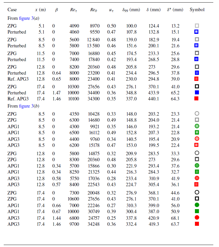

 x=xa
 x=xb
 x=xc

 x=x1
 x=x2
 Reτ

 u2¯+
 fϕuu+
 x=xa
 x=xb
 z+=0.4Reτ
 T+=4.8δ+/U∞+
 x=xb
 x=xc

 u2¯+
 fϕuu+
 x=x1
 x=x2
 fϕuu,Ref.APG3+−fϕuu,Perturbed+
 T+=4.8δ+/U∞+
 T+=2.4δ+/U∞+
 T+=350
 z+=0.4Reτ

 Reτ
 x=x1
 x=x2
 Reτ
 β

 x2
 x1
 x2
 x1
 fϕuu,x2+−fϕuu,x1+
 z/δ=0.4
 TU∞/δ=4.8
 TU∞/δ=2.4

 x=17.4
 Reτ≈10000
 β
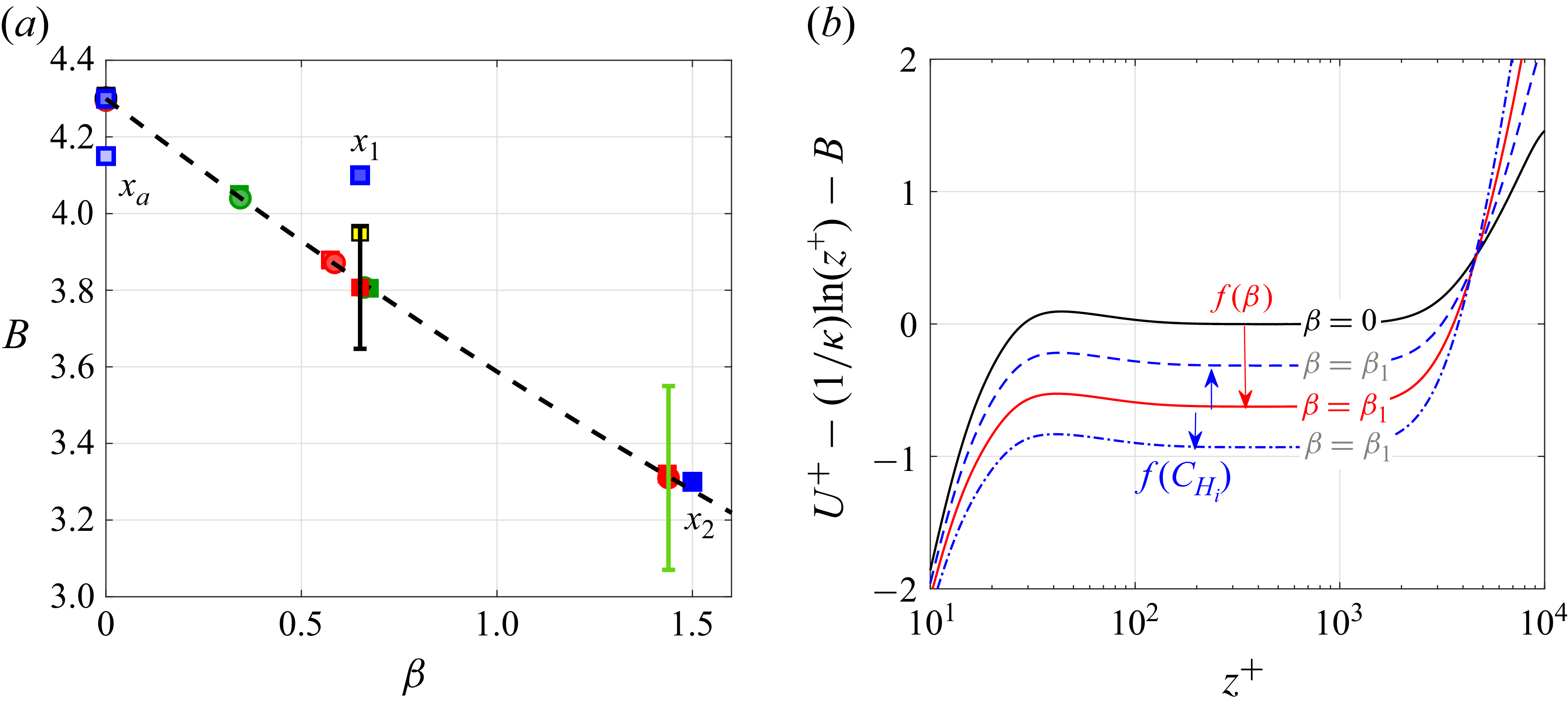
 B
 β
 Reτ
 β
 Reτ
 uτ
 β

 x=x1
 Reτ
 β
 Reτ
 β
 Reτ
 β
 Reτ
 1/κ
 ±5%

 CP


 Open access

