





1. Introduction
Geostrophic turbulence pervades the Earth’s ocean and planetary atmospheres, and plays an essential role in distributing solar energy from tropical to polar latitudes (Barry et al. Reference Barry, Craig and Thuburn2002) and mediating exchanges of physical and biogeochemical properties between coastal and open-ocean regions (Gruber et al. Reference Gruber, Lachkar, Frenzel, Marchesiello, Münnich, McWilliams, Nagai and Plattner2011; Thompson et al. Reference Thompson, Stewart, Spence and Heywood2018). Investigating the governing factors of geostrophic turbulent fluxes is therefore crucial to understanding and predicting the global biogeochemical cycles (Ruan et al. Reference Ruan, Couespel, Lévy, Li, Mak and Wang2023), the glacier retreat rates (Bennetts et al. Reference Bennetts2024; Dettling et al. Reference Dettling, Losch, Pollmann and Kanzow2024) and the Earth’s future climate state (Ferrari & Wunsch Reference Ferrari and Wunsch2009). Unlike its counterpart in the Earth’s atmosphere, geostrophic turbulence in the ocean, known collectively as mesoscale eddies, are characterised by order-of-magnitude separations of length scale from the external driving forcing of oceanic motions. This scale separation, in conjunction with limited computational power, renders the ocean component of state-of-the-art climate models too coarse in grid spacing to adequately resolve mesoscale eddies. Such a restriction on model resolution is particularly pronounced towards continental margins and high-latitude regions, where the ocean’s smallest mesoscale eddies are spawned and therefore must be parametrised (Hallberg Reference Hallberg2013; Stewart & Thompson Reference Stewart and Thompson2016).
Across continental margins and high-latitude ocean regions, the underlying sloping topography has been found to diminish the magnitude and alter the spatial structure of mesoscale eddy fluxes, which motivated recent empirical approaches to representing suppressed eddy fluxes based on the information of the bottom slope in primitive equation ocean models (Wang & Stewart Reference Wang and Stewart2020; Wei et al. Reference Wei, Wang, Stewart and Mak2022, Reference Wei, Wang and Mak2024; Dettling et al. Reference Dettling, Losch, Pollmann and Kanzow2024, Reference Dettling, Nakayama, Mensah and Losch2025; Nummelin & Isachsen Reference Nummelin and Isachsen2024; Sterl et al. Reference Sterl, Lacasce, Groeskamp, Nummelin, Isachsen and Baatsen2024); among these, diverging approaches were proposed for ‘retrograde’ (Wang & Stewart Reference Wang and Stewart2018, Reference Wang and Stewart2020) versus ‘prograde’ flows (Wei et al. Reference Wei, Wang, Stewart and Mak2022, Reference Wei, Wang and Mak2024), whose flow directions are opposite to and aligned with the intrinsic propagation direction of topographic Rossby waves, respectively (Poulin et al. Reference Poulin, Stegner, Hernández-Arencibia, Marrero-Díaz and Sangrà2014). In support of existing empirical approaches, the present work aims to investigate the physical mechanisms behind the dependencies of geostrophic eddy fluxes on a sloping bottom at the fundamental process-level. To this end, we use a reduced-order quasi-geostrophic (QG) model, which enables theoretical development and numerical validation across a broad range of physical parameter space.
The canonical theoretical framework of investigating geostrophic eddy dynamics across topography is the modified Eady (Blumsack & Gierasch Reference Blumsack and Gierasch1972) or Phillips (Mechoso Reference Mechoso1980) models, both of which incorporate a sloping bottom in their originally flat-bottomed counterparts. Blumsack & Gierasch (Reference Blumsack and Gierasch1972) and Mechoso (Reference Mechoso1980) calculated the linearly most unstable baroclinic waves to identify a key controlling parameter of the resulting baroclinic instabilities and heat fluxes: the ratio between the topographic and isopycnal slopes, denoted conventionally as the bottom slope parameter (Isachsen Reference Isachsen2011). The linear solutions of Blumsack & Gierasch (Reference Blumsack and Gierasch1972) and Mechoso (Reference Mechoso1980) have since been broadly applied to quantify the baroclinic instabilities of buoyant currents along continental shelves (Chen et al. Reference Chen, Chen and Lerczak2020) and heat fluxes across rim currents in convective ocean basins (Spall Reference Spall2004).
To evaluate the utility of linear theories in a nonlinear eddy field, Isachsen (Reference Isachsen2011) compared the eddy heat fluxes produced in a set of primitive equation simulations of baroclinic boundary currents with those predicted via the linear solutions of Blumsack & Gierasch (Reference Blumsack and Gierasch1972), and found qualitative discrepancies if the boundary current goes retrograde. Isachsen (Reference Isachsen2011) then attributed these discrepancies to the lack of nonlinear eddy–eddy interactions or interior background potential vorticity (PV) gradients in the modified linear Eady (Reference Eady1949) model. To investigate the impact of nonlinearity on eddy characteristics and fluxes, Deng & Wang (Reference Deng and Wang2024) ran a suite of two-layer QG turbulence simulations to show that eddies tend to be barotropised (de-barotropised) in retrograde (prograde) flow systems, thus strengthening (weakening) along-slope jet formation that eventually enhances (alleviates) topographic suppression on eddy fluxes across the topographic slope. In parallel, Lobo et al. (Reference Lobo, Griffies and Zhang2025) quantified the influences of interior PV gradients on baroclinic instabilities across a sloping bottom based on a linearised three-layer QG model, in which baroclinic instabilities and heat fluxes exhibited qualitatively similar dependencies on the sloping bottom to those found in primitive equation simulations of Isachsen (Reference Isachsen2011); some parameter dependencies (e.g. unchanging or even enhanced heat fluxes across an adequately strong topographic slope) are precluded by a two-layer linear QG model. However, it remains unclear how interior PV gradients and bottom topography may jointly regulate fully nonlinear eddy characteristics and fluxes.
To quantify the joint impacts from interior PV gradients and bottom topography on eddy characteristics and fluxes, a three-layer QG turbulence model with a sloping bottom serves as a minimum theoretical and numerical tool. In contrast to a two-layer QG model, a three-layer model captures the vertical structure of eddy buoyancy fluxes in tandem with a second baroclinic mode of eddy variability, both of which have been observed to regulate the mean state of ocean stratification and circulation, such as that in the Arctic Ocean (Zhao et al. Reference Zhao, Timmermans, Krishfield and Manucharyan2018; Manucharyan & Stewart Reference Manucharyan and Stewart2022). In the atmospheric literature, three-layer QG models have been employed to investigate the vertical structure of baroclinic instability in the Earth’s troposphere (Held & O’Brien Reference Held and O’Brien1992), given that such models can support both the Charney- and Eady-type baroclinic unstable waves (see §§ 6.1 and 8 of Isachsen Reference Isachsen2011). In the presence of a sloping bottom, three-layer QG models facilitated multiple past investigations of the linear stability properties of ocean boundary currents (Wright Reference Wright1980; Ikeda Reference Ikeda1983; Pichevin Reference Pichevin1998).
In this work, we extend previous investigations of three-layer QG flows by taking into account the fully developed turbulent state sustaining nonlinear eddy–eddy interactions, but focus specifically on the retrograde flow system. Both primitive equation ocean models (Isachsen Reference Isachsen2011) and linearised QG models (Lobo et al. Reference Lobo, Griffies and Zhang2025) showed that, in contrast to a prograde flow system, a retrograde flow system can be much more sensitive to the presence of an interior PV gradient, which results in qualitatively different eddy flux features spawned in a three-layer flow from those predicted by the linear theory of Blumsack & Gierasch (Reference Blumsack and Gierasch1972). Moreover, retrograde flow systems in the ocean frequently host undercurrents, whose formation was argued to be driven by up-gradient eddy buoyancy fluxes mediated by sloping topography (Wang & Stewart Reference Wang and Stewart2018; Capó et al. Reference Capó, McWilliams, Gula, Molemaker, Damien and Schubert2024), a process precluded by linear QG models. Previous QG turbulence models producing similarly up-gradient buoyancy fluxes over topography either evolved freely from initial random flow perturbations (Merryfield Reference Merryfield1998) or were driven by prescribed random forcing (Merryfield & Holloway Reference Merryfield and Holloway1999), which facilitated interpretations via equilibrium statistical mechanics (Bouchet & Venaille Reference Bouchet and Venaille2012; Venaille Reference Venaille2012). Here, we build our understanding upon the energetics and cascade phenomenology of geostrophic turbulence sustained by a background thermal shear (Salmon Reference Salmon1980) and mediated by a sloping bottom, which aid in adapting a predictive closure of eddy fluxes for two-layer, flat-bottomed QG turbulence (Chang & Held Reference Chang and Held2019, Reference Chang and Held2021) to a three-layer, sloping-bottomed retrograde flow system.
The remainder of this manuscript is structured as follows. In § 2, we detail the formulation of the three-layer QG turbulence model and formalise different variants of eddy fluxes in this model. In § 3, we postulate the theory of topographic impacts on fully developed turbulence in three-layer QG retrograde flows. In § 4, we outline the numerical implementation of our three-layer QG turbulence model and qualitatively validate our theory against the model diagnostics. In § 5, we adapt the closure theory of Chang & Held (Reference Chang and Held2021) based on the topographic impacts derived and validated in §§ 3 and 4 to arrive at a quantitative interpretation of eddy fluxes across sloping topography in our three-layer QG system. A parallel assessment on the original form of the closure theory is documented in Appendix B. Discussions of the connections between our results and previous studies, and the limitations of this work, are laid out in § 6. Concluding remarks follow in § 7.
2. Theory of three-layer QG turbulence
2.1. Three-layer QG model
Our investigation builds upon a three-layer QG model with a surface rigid lid and a meridionally and linearly sloping bottom posed on an
 $f$
-plane. The layerwise QG PV is formulated as (Vallis Reference Vallis2017; Manucharyan & Stewart Reference Manucharyan and Stewart2022)
 \begin{align} &\qquad Q_{1} = {\nabla} ^{2}\varPsi _{1} + \frac {f_{0}^{2}}{g'_{3/2}H_{1}} \left (\varPsi _{2} - \varPsi _{1}\right )\!, \\[-12pt]\nonumber \end{align}
 \begin{align} Q_{2} = & {\nabla} ^{2}\varPsi _{2} + \frac {f_{0}^{2}}{g'_{3/2}H_{2}}\left (\varPsi _{1} - \varPsi _{2}\right ) + \frac {f_{0}^{2}}{g'_{5/2}H_{2}}\left (\varPsi _{3} - \varPsi _{2}\right )\!, \\[-12pt]\nonumber \end{align}
 \begin{align} &Q_{3} = {\nabla} ^2\varPsi _{3} + \frac {f_{0}^{2}}{g'_{5/2}H_{3}}\left (\varPsi _{2} - \varPsi _{3}\right ) + \frac {f_{0}}{H_{3}}\eta _{b}, \end{align}
where
 $\boldsymbol{\nabla}$
denotes the horizontal gradient operator,
 $\varPsi _{i}$
represents the total geostrophic streamfunction,
 $f_{0}$
stands for the Coriolis frequency,
 $H_{i}$
measures the resting layer thickness with
 $i=1,\,2,\,3$
denoting the layer index,
 $g'_{j}$
signifies the reduced gravity across the upper (with interfacial index
 $j = 3/2$
) and lower (with
 $j = 5/2$
) isopycnal interfaces, and
 $\eta _{b}$
denotes the linear topographic elevation shoaling poleward of the model domain.
Following previous QG studies (Held & O’Brien Reference Held and O’Brien1992; Lobo et al. Reference Lobo, Griffies and Zhang2025), a vertically sheared eastward background flow is prescribed to fuel QG turbulence via baroclinic instabilities. Specifically, the background flow and the corresponding vertical shear are prescribed as
 \begin{align} U_{1} &= 2U, \\[-12pt]\nonumber \end{align}
 \begin{align} U_{2} &= \frac {2}{\left (\alpha +1\right )}U, \\[-12pt]\nonumber \end{align}
 \begin{align} U_{3} &= 0, \\[-12pt]\nonumber \end{align}
 \begin{align} U_{1} - U_{2} &= \frac {2\alpha }{\alpha + 1}U,\quad U_{2} - U_{3} = \frac {2}{\alpha +1}U, \end{align}
where
 $\alpha = (U_{1} - U_{2})/(U_{2} - U_{3})$
measures the ratio of the background thermal shears across the upper and lower isopycnal interfaces. Following Lobo et al. (Reference Lobo, Griffies and Zhang2025), we define
 $\alpha$
formally as the shear parameter and keep its value positive definite throughout this work. In addition, we define a three-layer QG model as a surface-driven (bottom-driven) system if
 $\alpha$
is larger (smaller) than unity (see figures 1
a and 1
c). The two systems are delineated by the special case of
 $\alpha = 1$
(see figure 1
b), corresponding to a linearly varying background thermal shear and therefore a vertically discretised Eady-like model. Note from (2.2d
) that the total thermal shear remains fixed at
 $2U$
across the full fluid column and that the shear parameter merely adjusts the vertical distribution of the background shear (Held & O’Brien Reference Held and O’Brien1992).
Decomposing the total streamfunction into a background mean and an eddy part, we rewrite the layerwise QG PV as
 \begin{align} Q_{1} = &\frac {f_{0}^{2}}{g'_{3/2}H_{1}}\left (U_{1} - U_{2}\right )y + q_{1}, \\[-12pt]\nonumber\end{align}
 \begin{align} Q_{2} = &\frac {f_{0}^{2}}{g'_{3/2}H_{2}}\left (U_{2} - U_{1}\right )y + \frac {f_{0}^{2}}{g'_{5/2}H_{2}}\left (U_{2} - U_{3}\right )y +q_{2}, \\[-12pt]\nonumber \end{align}
 \begin{align} Q_{3} = &\frac {f_{0}^{2}}{g'_{5/2}H_{3}}\left (U_{3} - U_{2}\right )y + \frac {f_{0}}{H_{3}}\eta _{b} + q_{3}, \end{align}
where
 $q_{i}$
stands for the layerwise eddy QG PV and is related to the eddy streamfunction
 $\psi _{i}$
through
 \begin{align} q_{1} = &{\nabla} ^{2}\psi _{1} + \frac {f_{0}^{2}}{g'_{3/2}H_{1}}\left (\psi _{2} - \psi _{1}\right )\!, \\[-12pt]\nonumber \end{align}
 \begin{align} q_{2} = &{\nabla} ^{2}\psi _{2} +\frac {f_{0}^{2}}{g'_{3/2}H_{2}}\left (\psi _{1} - \psi _{2}\right ) + \frac {f_{0}^{2}}{g'_{5/2}H_{2}}\left (\psi _{3} - \psi _{2}\right )\!, \\[-12pt]\nonumber \end{align}
 \begin{align} q_{3} = &{\nabla} ^2\psi _{3} + \frac {f_{0}^{2}}{g'_{5/2}H_{3}}\left (\psi _{2} - \psi _{3}\right )\!. \end{align}
The prescribed background thermal shear provides an infinite well of available potential energy to sustain baroclinic turbulence. To arrive at a statistically steady state, dissipation must be added at both large scales to dissipate energy and small scales to remove potential enstrophy filaments (Gallet & Ferrari Reference Gallet and Ferrari2020). In particular, we employ a quadratic bottom drag in tandem with a hyperviscosity in our model. The governing equation for the forced-dissipative three-layer QG system dictates the material conservation of QG PV, formulated as
 \begin{align} \begin{split} \frac {\partial Q_{i}}{\partial t} & + J\left (\varPsi _{i},\,Q_{i}\right ) = -\nu {\nabla} ^{8}Q_{i} \\ &- \delta _{i3}C_{d}\left [\partial _{x}\left (\left |\boldsymbol{\nabla }\varPsi _{3}\right |\partial _{x}\varPsi _{3}\right ) + \partial _{y}\left (\left |\boldsymbol{\nabla }\varPsi _{3}\right |\partial _{y}\varPsi _{3}\right )\right ]\!, \end{split} \end{align}
where
 $J(A,\,B) = \partial _{x}A\,\partial _{y}B - \partial _{y}A\,\partial _{x}B$
denotes the Jacobian operator,
 $\nu$
signifies the hyperviscous coefficient,
 $\delta$
stands for the Kronecker delta and
 $C_{d}$
represents the bottom quadratic drag coefficient. Note that
 $C_{d}$
has a dimension of inverse length scale (Grianik et al. Reference Grianik, Held, Smith and Vallis2004; Kong & Jansen Reference Kong and Jansen2017) and that its product with an ocean bottom boundary layer thickness yields the more conventional non-dimensional drag coefficient adopted in primitive equation ocean models (Arbic & Scott Reference Arbic and Scott2008).
2.2. Modal decomposition
Further insights of turbulent eddy properties can be gained via modal decomposition of eddy motions (Smith & Vallis Reference Smith and Vallis2001, Reference Smith and Vallis2002; Manucharyan & Stewart Reference Manucharyan and Stewart2022). This decomposition amounts to seeking solutions to the Sturm–Liouville eigenvalue problem, which in a three-layer QG system reads (Manucharyan & Stewart Reference Manucharyan and Stewart2022)
 \begin{align} &\frac {f_{0}^{2}}{H_{1}}\left (\frac {\psi _{2} - \psi _{1}}{g'_{3/2}}\right ) = -\varUpsilon \psi _{1}, \\[-12pt]\nonumber \end{align}
 \begin{align} \frac {f_{0}^{2}}{H_{2}} & \left (\frac {\psi _{1} - \psi _{2}}{g'_{3/2}} + \frac {\psi _{3} - \psi _{2}}{g'_{5/2}} \right ) = -\varUpsilon \psi _{2}, \\[-12pt]\nonumber \end{align}
 \begin{align} &\quad \frac {f_{0}^{2}}{H_{3}}\left (\frac {\psi _{2} - \psi _{3}}{g'_{5/2}}\right ) = -\varUpsilon \psi _{3}, \end{align}
where
 $\varUpsilon$
denotes the eigenvalue.
In this work, we make a simplification by considering a uniformly stratified flow, i.e.
 \begin{align} H_{1} = H_{2} = H_{3} = H, \\[-12pt]\nonumber \end{align}
 \begin{align} g'_{3/2} = g'_{5/2} = g'. \end{align}
This simplification is motivated by the fact that even for linear stability analysis, it is impractical to survey a complete range of parameter space accommodated by a three-layer QG model (Pichevin Reference Pichevin1998; Olascoaga Reference Olascoaga2001; Lobo et al. Reference Lobo, Griffies and Zhang2025). In such a model with a sloping bottom, independent parameters include the ratio of reduced gravities across the two isopycnal interfaces, two ratios of resting layer thicknesses, the ratio of the two isopycnal interface slopes, the steepness of the bottom slope and the bottom drag strength (Olascoaga Reference Olascoaga2001; Lobo et al. Reference Lobo, Griffies and Zhang2025), hence, amounting to at least six controlling parameters. Among these, the isopycnal slope ratio and the topographic slope were identified as key parameters to the properties of baroclinic instabilities (Pichevin Reference Pichevin1998; Lobo et al. Reference Lobo, Griffies and Zhang2025). We therefore choose to co-vary the isopycnal slope ratio and the topographic slope, in addition to independently adjusting the bottom drag strength, but suppress any additional degrees of freedom in this work.
We note that our choice of parameter space is similar to that of Lobo et al. (Reference Lobo, Griffies and Zhang2025). Specifically, Lobo et al. (Reference Lobo, Griffies and Zhang2025) fixed the resting layer thicknesses and reduced gravities in their three-layer model, and co-varied the isopycnal slope ratio and the topographic slope, although Lobo et al. (Reference Lobo, Griffies and Zhang2025) considered surface-intensified stratification and adopted a fixed linear drag strength. Moreover, our choice of uniform stratification could be partly justified by observations that ocean stratification is more vertically uniform at high latitudes (Arbic & Flierl Reference Arbic and Flierl2004) and that topographic impacts can dominate over the influences of weak stratification on baroclinic eddies in these regions (Isachsen Reference Isachsen2011). Nevertheless, the limitations of our chosen parameter space are discussed in § 6.4.
With vertically uniform stratification, the eigenvalues to (2.6) are
 \begin{align} \varUpsilon _{0} = 0,\quad \varUpsilon _{1} = \frac {f_{0}^{2}}{g'H},\quad \varUpsilon _{2} = 3\frac {f_{0}^{2}}{g'H}, \end{align}
and the corresponding eigenvectors are
 \begin{align} &\qquad \quad e_{0} = \left (1,\,1,\,1\right )\!, \\[-12pt]\nonumber \end{align}
 \begin{align} &\quad e_{1} = \left (-\sqrt {3/2},\,0,\,\sqrt {3/2}\right )\!, \\[-12pt]\nonumber \end{align}
 \begin{align} &e_{2} = \left (-\sqrt {2}/2,\,\sqrt {2},\,-\sqrt {2}/2\right )\!. \end{align}
The eigenvectors in (2.9) are mutually orthogonal, which guide the modal projections of the eddy or mean variables following Smith & Vallis (Reference Smith and Vallis2001, Reference Smith and Vallis2002). Thus, the vertical normal modes of eddy streamfunctions are defined by
 \begin{align} \psi = \frac {1}{3}\left (\psi _{1} + \psi _{2} + \psi _{3}\right )\!, \\[-12pt]\nonumber \end{align}
 \begin{align} \tau _{1} = \frac {1}{\sqrt {6}}\left (\psi _{3} - \psi _{1}\right )\!, \\[-12pt]\nonumber \end{align}
 \begin{align} \tau _{2} = \frac {\sqrt {2}}{6}\left (2\psi _{2} - \psi _{1} - \psi _{3}\right )\!, \end{align}
where
 $\psi$
,
 $\tau _{1}$
and
 $\tau _{2}$
stand for streamfunctions of the barotropic mode, the first baroclinic mode and the second baroclinic mode, respectively. Meanwhile, the first and second baroclinic Rossby deformation radii are respectively expressed as
 \begin{align} R_{d1} = \frac {\sqrt {g'H}}{f_{0}} =\frac {1}{\sqrt {\varUpsilon _{1}}}, \\[-12pt]\nonumber \end{align}
 \begin{align} R_{d2} = \frac {1}{\sqrt {3}}\frac {\sqrt {g'H}}{f_{0}} =\frac {1}{\sqrt {\varUpsilon _{2}}}. \end{align}
The above-mentioned modal decomposition offers a complete projection of the geostrophic flow in a three-layer QG model (Gill Reference Gill1982; Smith & Vallis Reference Smith and Vallis2001, Reference Smith and Vallis2002; LaCasce Reference LaCasce2017), which facilitated analyses of eddy energetics and nonlinear eddy fluxes in three-layer QG turbulence (Manucharyan & Stewart Reference Manucharyan and Stewart2022). In the presence of sloping bathymetry, alternative approaches have been proposed to complement or revise the above-mentioned modal decomposition. We refer the reader to Yassin (Reference Yassin2021) and Yassin & Griffies (Reference Yassin and Griffies2022) for a mathematically rigorous presentation of geostrophic modal decompositions in a continuously stratified ocean with arbitrary vertical boundary conditions. In practice, these alternative approaches have facilitated an understanding of the vertical structures of geostrophic motions (de La Lama et al. Reference de La Lama, LaCasce and Fuhr2016; Zhang & Wolfe Reference Zhang and Wolfe2022; Zhang et al. Reference Zhang, Griffies, Hallberg, Kuo and Wolfe2024). However, how bathymetry-dependent modal decompositions may unveil the dynamics of fully developed geostrophic turbulence, to be detailed subsequently, is unclear.
In a baroclinic QG system, the difference between eddy streamfunctions across two adjacent isopycnal layers are linearly related to the vertical fluctuation of the corresponding isopycnal interface (see §§ 5.3.2, 5.4.6 and 10.3.3 of Vallis Reference Vallis2017), whose additive inverse informs the eddy buoyancy or temperature anomaly associated with baroclinic turbulence (Chang & Held Reference Chang and Held2019, Reference Chang and Held2021; Gallet & Ferrari Reference Gallet and Ferrari2020, Reference Gallet and Ferrari2021). These relations in our three-layer QG model are formalised as
 \begin{align} \eta _{3/2} = \frac {f_0}{g^{^\prime }}\left (\psi _{2} - \psi _{1}\right ) = - \frac {H}{g^{^\prime }}b_{3/2}, \\[-12pt]\nonumber \end{align}
 \begin{align} \eta _{5/2} = \frac {f_0}{g^{^\prime }}\left (\psi _{3} - \psi _{2}\right ) = - \frac {H}{g^{^\prime }}b_{5/2}, \\[12pt] \nonumber \end{align}
where
 $\eta _{j}$
and
 $b_{j}$
are the isopycnal height anomaly and the associated buoyancy anomaly, respectively, defined with respect to the mean vertical levels of isopycnal interfaces. In our uniformly stratified model, these mean isopycnal vertical levels are measured by
 \begin{align} \mathcal{H}_{3/2}(y) = S_{3/2}\boldsymbol{\cdot }y - H, \\[-12pt]\nonumber \end{align}
 \begin{align} \mathcal{H}_{5/2}(y) = S_{5/2}\boldsymbol{\cdot }y - 2H, \end{align}
whose meridional variations are governed by the mean isopycnal slopes:
 \begin{align} S_{3/2} = \frac {f_{0}}{g^{^\prime }}(U_{1} - U_{2}),\quad S_{5/2} = \frac {f_{0}}{g^{^\prime }}(U_{2} - U_{3}). \end{align}
Comparing (2.12) with the modal eddy streamfunctions defined in (2.10), we note that the two baroclinic modes are related to the isopycnal interface fluctuations through
 \begin{align} \tau _{1} = \frac {1}{\sqrt {6}}\frac {g^{^\prime }}{f_{0}}\left (\eta _{3/2} + \eta _{5/2}\right )\!, \\[-12pt]\nonumber \end{align}
 \begin{align} \tau _{2} = \frac {\sqrt {2}}{6}\frac {g^{^\prime }}{f_{0}}\left (\eta _{3/2} - \eta _{5/2}\right )\!, \end{align}
which intuitively show that the first baroclinic mode quantifies the vertically integrated buoyancy anomaly and that the second baroclinic mode measures the thickness anomaly confined to the middle isopycnal layer. Previous studies using primitive equation simulations frequently quantified eddy fluxes associated with
 $\tau _1$
, but neglected those of
 $\tau _2$
(e.g. Wang & Stewart Reference Wang and Stewart2020), the latter of which, as shown later, plays a fundamental role in the eddy energetic pathways and the vertical structure of baroclinic eddy fluxes over a sloping bottom.
2.3. Non-dimensionalisation and controlling parameters
To achieve a systematic parameter sweep, we non-dimensionalise the QG PV equations and identify the controlling parameters. To this end, we employ the first Rossby deformation radius
 $R_{d1}$
as the characteristic length scale and the prescribed thermal shear
 $U$
as the characteristic velocity scale. Hence, the Eady time scale, i.e.
 $T_{\textit{Eady}} = R_{d1}/U$
, emerges as characteristic time scale. The non-dimensionalised QG PV equations then read
 \begin{align} &\frac {\partial q_{1}^*}{\partial t^*} + 2\frac {\partial q_{1}^*}{\partial x^*} + \frac {2\alpha }{\left (\alpha + 1\right )}\frac {\partial \psi _{1}^*}{\partial x^*} + J^*\left (\psi _{1}^*,\,q_{1}^*\right ) = -\nu ^*{\nabla} ^{*8}q_{1}^*, \\[-12pt]\nonumber \end{align}
 \begin{align} &\frac {\partial q_{2}^*}{\partial t^*} + \frac {2}{\left (\alpha + 1\right )}\frac {\partial q_{2}^*}{\partial x^*} + \frac {2-2\alpha }{\left (\alpha + 1\right )}\frac {\partial \psi _{2}^*}{\partial x^*} + J^*\left (\psi _{2}^*,\,q_{2}^*\right ) = -\nu ^*{\nabla} ^{*8}q_{2}^*, \\[-12pt]\nonumber \end{align}
 \begin{align} &\frac {\partial q_{3}^*}{\partial t^*} + \frac {-2\left [1-\left (S_{\textit{topo}}/S_{5/2}\right )\right ]}{(\alpha + 1)}\frac {\partial \psi _{3}^*}{\partial x^*} + J^*\left (\psi _{3}^*,\,q_{3}^*\right ) \\ &= -\nu ^*{\nabla} ^{*8}q_{3}^* - C_{d}^*\left [\partial _{x^*}\left (\left |{\nabla} ^*\psi _{3}^*\right |\partial _{x^*}\psi _{3}^*\right ) + \partial _{y^*}\left (\left |{\nabla} ^*\psi _{3}^*\right |\partial _{y^*}\psi _{3}^*\right )\right ]\!, \end{align}
with the non-dimensionalised QG PV formulated as
 \begin{align} &q_{1}^* = {\nabla} ^2\psi _{1}^* + \left (\psi _{2}^* - \psi _{1}^*\right )\!, \\[-12pt]\nonumber \end{align}
 \begin{align} &q_{2}^* = {\nabla} ^2\psi _{2}^* + \left (\psi _{1}^* + \psi _{3}^* - 2\psi _{2}^*\right )\!, \\[-12pt]\nonumber \end{align}
 \begin{align} &q_{3}^* = {\nabla} ^2\psi _{3}^* + \left (\psi _{2}^* - \psi _{3}^*\right )\!, \end{align}
where
 $\bullet ^*$
denotes a non-dimensionalised variable and
 $S_{\textit{topo}}$
is the topographic slope.
In addition to the shear parameter
 $\alpha$
, (2.16) identifies three environmental parameters: the quadratic drag coefficient, the hyperviscous coefficient and the topographic slope parameter, defined respectively as
 \begin{align} &C_{d}^* = C_{d}\boldsymbol{\cdot }R_{d1}, \\[-12pt]\nonumber \end{align}
 \begin{align} &\nu ^* = \frac {\nu }{U\boldsymbol{\cdot }R_{d1}^{7}}, \\[-12pt]\nonumber \end{align}
 \begin{align} S_{\textit{topo}}\big /S_{5/2} &= \frac {\partial _{y}\eta _{b}}{\left [2U\big /\left (\alpha + 1\right )\right ]f_{0}\big /g'}. \end{align}
Note that the emergent topographic slope parameter,
 $S_{\textit{topo}}/S_{5/2}$
, measures the ratio of topographic and lower isopycnal interface slopes, and thus differs from its variant formulated using the depth-mean isopycnal slopes in previous studies (e.g. Isachsen Reference Isachsen2011; Wang & Stewart Reference Wang and Stewart2020), which, in our three-layer QG model, is equivalent to a non-dimensionalised barotropic PV gradient independent of the shear parameter,
 \begin{align} G_{{bt}}^* = \frac {2}{3\left (S_{3/2}+S_{5/2}\right )}S_{\textit{topo}} = \frac {g^{^\prime }}{3f_{0}U}S_{\textit{topo}}, \end{align}
where the factor of
 $1/3$
sources from a depth-average of the bottom-layer topographic PV gradient. In addition, subject to uniform stratification, the ratio of interior isopycnal slopes becomes identical to the shear parameter (i.e.
 $S_{3/2}/S_{5/2} = \alpha$
).
In summary, a three-layer QG turbulence system defined in (2.16)–(2.17) would be governed by the topographic slope parameter (
 $S_{\textit{topo}}/S_{5/2}$
), or alternatively, the barotropic PV gradient (
 $G_{{bt}}^*$
), in addition to the shear parameter (
 $\alpha$
) and the bottom drag strength (
 $C_{d}^*$
), provided that the hyperviscous effect is negligible and the model domain is adequately large.
2.4. Eddy buoyancy and PV fluxes
Central to understanding a fully developed turbulent eddy field are the parameter dependencies of eddy fluxes. In a three-layer QG turbulence model, there are several dynamically linked variants of eddy fluxes, which are formalised in the present and the following sections.
We note first from (2.12) that the eddy buoyancy fluxes, or equivalently, the interfacial eddy form stresses, can be quantified as (Lobo et al. Reference Lobo, Griffies and Zhang2025)
 \begin{align} \begin{split} \left \langle v_{3/2}\boldsymbol{\cdot }b_{3/2}\right \rangle &= \frac {f_{0}}{H}\left \langle \frac {v_{1}+v_{2}}{2}\boldsymbol{\cdot }\left (\psi _{1} - \psi _{2}\right )\right \rangle \\ &= -\frac {f_{0}}{H}\left \langle v_{1}\boldsymbol{\cdot }\psi _{2}\right \rangle = -\frac {g^{^\prime }}{f_{0}}\left \langle v_{1}\boldsymbol{\cdot }q_{1}\right \rangle \!, \end{split} \\[-12pt]\nonumber \end{align}
 \begin{align} \begin{split} \left \langle v_{5/2}\boldsymbol{\cdot }b_{5/2}\right \rangle &= \frac {f_{0}}{H}\left \langle \frac {v_{2}+v_{3}}{2}\boldsymbol{\cdot }\left (\psi _{2} - \psi _{3}\right )\right \rangle \\ &= \frac {f_{0}}{H}\left \langle v_{3}\boldsymbol{\cdot }\psi _{2}\right \rangle = \frac {g^{^\prime }}{f_{0}}\left \langle v_{3}\boldsymbol{\cdot }q_{3}\right \rangle \!, \end{split} \\[12pt] \nonumber \end{align}
where
 $v$
represents the meridional eddy velocity, defined either within an isopycnal layer (indicated by
 $v_{i}$
with
 $i = 1,\,2,\,3$
) or at the mean vertical level of an isopycnal interface (indicated by
 $v_{j}$
with
 $j = 3/2$
or
 $5/2$
), and
 $\left \langle \bullet \right \rangle$
stands for the domain-average operator. In deriving (2.20), we have repeatedly used doubly periodic boundary conditions and invoked vanishing relative vorticity fluxes upon domain-average (Held & O’Brien Reference Held and O’Brien1992). For the ease of reference, we further non-dimensionalise and temporally average (2.20) as
 \begin{align} \overline {\left \langle v_{3/2}^*\boldsymbol{\cdot }b_{3/2}^* \right \rangle } = -\overline {\left \langle v_{1}^*\boldsymbol{\cdot }q_{1}^*\right \rangle }\!, \\[-12pt]\nonumber \end{align}
 \begin{align} \overline {\left \langle v_{5/2}^*\boldsymbol{\cdot }b_{5/2}^* \right \rangle } = \overline {\left \langle v_{3}^*\boldsymbol{\cdot }q_{3}^*\right \rangle }\!, \end{align}
where
 $\overline {\bullet }$
denotes the time-average operator.
It is clear from (2.21) that eddy buoyancy fluxes in a three-layer QG system are convertible with the eddy PV fluxes in the upper and lower isopycnal layers. Given that eddy PV fluxes in a baroclinic QG system are strictly constrained by the Taylor–Bretherton relation (Held & O’Brien Reference Held and O’Brien1992; Smith & Vallis Reference Smith and Vallis2002; Meunier et al. Reference Meunier, Miquel and Gallet2023a
,
Reference Meunier, Miquel and Galletb
), i.e. the vertically integrated eddy PV fluxes identically vanish (
 $\sum _{i=1}^{3}\langle v_{i}\boldsymbol{\cdot }q_{i}\rangle \boldsymbol{\cdot }H_{i} = 0$
), all variants of eddy fluxes, defined so far and subsequently, carry only two degrees of freedom in a three-layer QG model.
Next, to see the dynamical relevance of eddy PV fluxes in the middle isopycnal layer, we formulate the non-dimensional turbulent energy budget of the forced-dissipative three-layer QG model, by multiplying the layerwise eddy streamfunction (
 $\psi _{i}^*$
) with the corresponding QG PV conservation (2.16), and then taking a domain- and depth-average to arrive at
 \begin{align} \begin{split} &\frac {1}{3}\frac {\partial }{\partial t^*}\left \langle \sum _{i=1}^{3}\frac {\left |\boldsymbol{\nabla }\psi _{i}^*\right |^{2}}{2} + \frac {\left (\psi _{1}^* - \psi _{2}^*\right )^{2}}{2} + \frac {\left (\psi _{2}^* - \psi _{3}^*\right )^{2}}{2}\right \rangle \\ &= -\frac {2}{3}\left \langle v_{1}^*\boldsymbol{\cdot }q_{1}^*\right \rangle - \frac {2}{3(\alpha + 1)}\left \langle v_{2}^*\boldsymbol{\cdot }q_{2}^*\right \rangle + \mathrm{Dissipation}. \end{split} \end{align}
By further averaging (2.22) temporally, the non-dimensional turbulent energy injection rate, to be balanced by dissipation in a statistically steady state, is formally quantified as
 \begin{align} \varepsilon _{p}^* = -\frac {2}{3}\overline {\left \langle v_{1}^*\boldsymbol{\cdot }q_{1}^*\right \rangle } - \frac {2}{3(\alpha + 1)}\overline {\left \langle v_{2}^*\boldsymbol{\cdot }q_{2}^*\right \rangle }. \end{align}
Equation (2.23) shows that
 $\varepsilon _{p}^*$
can be inferred directly from eddy PV fluxes in the upper and middle isopycnal layers, in conjunction with the background shear parameter.
2.5. Modal energetics and eddy fluxes
Apart from analysing the layerwise PV dynamics, one may formalise eddy fluxes that quantify the interactions between barotropic and baroclinic modes, which, as shown later, are key to understanding the topographic impacts on fully developed turbulence. To wit, we recast the QG PV conservation (2.16) into its modal form based on the modal streamfunctions defined in (2.10); this amounts to a linear combination of the layerwise QV PV equations, weighted by each eigenvector in (2.9), followed by a depth average:
 \begin{align} \begin{split} \frac {\partial {\nabla} ^2\psi ^*}{\partial t^*} &+ \frac {2(\alpha + 2)}{3(\alpha + 1)}\frac {\partial {\nabla} ^2\psi ^*}{\partial x^*} - \frac {\sqrt {6}}{3}\frac {\partial {\nabla} ^2\tau _{1}^*}{\partial x^*} + \frac {\sqrt {2}(1 - \alpha )}{3(1 + \alpha )}\frac {\partial {\nabla} ^2\tau _{2}^*}{\partial x^*} \\&+ J(\psi ^*,{\nabla} ^2\psi ^*) + J(\tau _{1}^*,{\nabla} ^2\tau _{1}^*) + J(\tau _{2}^*,{\nabla} ^2\tau _{2}^*) \\&= \underbrace {-\frac {2}{3\left (\alpha + 1\right )}\frac {S_{\textit{topo}}}{S_{5/2}}\frac {\partial }{\partial x^*}\left (\psi ^* + \frac {\sqrt {6}}{2}\tau _{1}^* - \frac {\sqrt {2}}{2}\tau _{2}^*\right )}_{\mathrm{Topo\,on\,BT}} + \mathrm{Dissipation}, \end{split} \end{align}
 \begin{align} \begin{split} \frac {\partial \left ({\nabla} ^2\tau _{1}^* - \tau _{1}^*\right )}{\partial t^*} &- \frac {2}{\sqrt {6}}\frac {\partial {\nabla} ^2\psi ^*}{\partial x^*} + \frac {\partial {\nabla} ^2\tau _{1}^*}{\partial x^*} + \frac {1}{\sqrt {3}}\frac {\partial {\nabla} ^2\tau _{2}^*}{\partial x^*} - \frac {2}{(\alpha + 1)}\frac {\partial \tau _{1}^*}{\partial x^*} \\&+ J(\psi ^*,{\nabla} ^2\tau _{1}^* - \tau _{1}^*) + J(\tau _{1}^*,{\nabla} ^2\psi ^*) - \frac {1}{\sqrt {2}}J(\tau _{1}^*,{\nabla} ^2\tau _{2}^*) - \frac {1}{\sqrt {2}}J(\tau _{2}^*,{\nabla} ^2\tau _{1}^*) + \sqrt {2}J(\tau _{1}^*,\tau _{2}^*) \\&= \underbrace {\frac {2}{\sqrt {6}}\frac {\partial }{\partial x^*}\big (\psi ^* + \sqrt {2}\tau _{2}^*\big )}_{\mathrm{BT}/\mathrm{BC2\,on\,BC1}} \underbrace {-\frac {2}{\sqrt {6} (\alpha + 1)}\frac {S_{\textit{topo}}}{S_{5/2}}\frac {\partial }{\partial x^*}\left (\psi ^* + \frac {\sqrt {6}}{2}\tau _{1}^* - \frac {\sqrt {2}}{2}\tau _{2}^* \right )}_{\mathrm{Topo\,on\,BC1}} + \mathrm{Dissipation}, \end{split} \end{align}
 \begin{align} \begin{split} \frac {\partial \left ({\nabla} ^2\tau _{2}^* - 3\tau _{2}^*\right )}{\partial t^*} &+ \frac {\sqrt {2}(1-\alpha )}{3(1 + \alpha )}\frac {\partial {\nabla} ^2\psi ^*}{\partial x^*} + \frac {1}{\sqrt {3}}\frac {\partial {\nabla} ^2\tau _{1}^*}{\partial x^*} + \frac {(\alpha + 5)}{3(\alpha + 1)}\frac {\partial {\nabla} ^2\tau _{2}^*}{\partial x^*} - \frac {2\alpha + 4}{\alpha +1}\frac {\partial \tau _{2}^*}{\partial x^*} \\& + J(\psi ^*,{\nabla} ^2\tau _{2}^* - 3\tau _{2}^*) + J(\tau _{2}^*,{\nabla} ^2\psi ^*) + \frac {1}{\sqrt {2}}J(\tau _{2}^*,{\nabla} ^2\tau _{2}^*) - \frac {1}{\sqrt {2}}J(\tau _{1}^*,{\nabla} ^2\tau _{1}^*) \\&= \underbrace {-\frac {\sqrt {2}(1-\alpha )}{1+\alpha }\frac {\partial \psi ^*}{\partial x^*}}_{\mathrm{BT\,on\,BC2}} \underbrace {+\frac {\sqrt {2}}{3}\frac {1}{1+\alpha }\frac {S_{\textit{topo}}}{S_{5/2}}\frac {\partial }{\partial x^*}\left (\psi ^* + \frac {\sqrt {6}}{2}\tau _{1}^* - \frac {\sqrt {2}}{2}\tau _{2}^* \right )}_{\mathrm{Topo\,on\,BC2}} + \mathrm{Dissipation}. \end{split} \end{align}
Here, we have annotated several key terms related to the sources of modal eddy variability and the presence of topography. For instance, ‘Topo on BT’ measures the tendency of barotropic eddy PV due to topographically induced modal interactions, whereas ‘BT/BC2 on BC1’ quantifies the tendency of the first baroclinic mode resulting from the barotropic or second baroclinic modes stirring the background thermal shear. All unannotated terms in (2.24) represent self- or cross-modal interactions without topographic rectification or stirring of the background thermal shear. Throughout this work, we use the term ‘topographic rectification’ to indicate the modulating effects of a sloping bottom on geostrophic modal interactions, turbulent energy cycling and eddy fluxes within a retrograde thermal shear.
To simplify analysis, we formulate the modal form of total turbulent energy budget by multiplying (2.24) with the corresponding modal eddy streamfunctions and then taking the sum,
 \begin{align} \begin{split} &\frac {\partial }{\partial t^*}\left \langle \frac {1}{2}\left (\left |\boldsymbol{\nabla }\psi ^*\right |^2+\left |\boldsymbol{\nabla }\tau _{1}^*\right |^2 + \tau _{1}^{*2} +\left |\boldsymbol{\nabla }\tau _{2}^*\right |^2+3\tau _{2}^{*2}\right )\right \rangle \\ &= \underbrace {-\frac {\sqrt {6}}{3}\left \langle \partial _{x^*}\psi ^*\boldsymbol{\cdot }\tau _{1}^*\right \rangle - \frac {2\sqrt {3}}{3}\,\left \langle \partial _{x^*}\tau _{2}^*\boldsymbol{\cdot }\tau _{1}^*\right \rangle }_{\mathrm{BC1\,source}} \\ &\underbrace {-\frac {\sqrt {2}\left (\alpha - 1\right )}{\left (\alpha + 1\right )}\left \langle \partial _{x^*}\psi ^*\boldsymbol{\cdot }\tau _{2}^*\right \rangle }_{\mathrm{BC2\,source}}\\ &+\mathrm{Dissipation}, \end{split} \end{align}
where the source terms of the first and second baroclinic modal eddy energy due to the reservoir of available potential energy have been highlighted, labelled ‘BC1 source’ and ‘BC2 source’, respectively. These energy source terms stem precisely from the annotated terms in the modal eddy PV budgets in (2.24) that account for the stirring of the background thermal shear; the thermal shear is concealed in the energy budget via our non-dimensionalisation. A comparison between (2.24) and (2.25) implies that a sloping bottom neither produces nor dissipates the total energy, but can redistribute energy across different modes. This topographically induced energy transfer was theorised using a two-layer QG turbulence model by Deng & Wang (Reference Deng and Wang2024), and will be formalised for a three-layer QG system in subsequent sections.
Temporally averaging the total turbulent energy budget (2.25) yields the total energy injection rate in its modal form:
 \begin{align} \begin{split} \varepsilon _{p}^* = &\underbrace {-\frac {\sqrt {6}}{3}\overline {\left \langle \partial _{x^*}\psi ^*\boldsymbol{\cdot }\tau _{1}^*\right \rangle }}_{\mathrm{BT\,on\,BC1}} \quad \underbrace {- \frac {\sqrt {2}\left (\alpha - 1\right )}{\left (\alpha + 1\right )}\overline {\left \langle \partial _{x^*}\psi ^*\boldsymbol{\cdot }\tau _{2}^*\right \rangle }}_{\mathrm{BT\,on\,BC2}}\\ &\underbrace {- \frac {2\sqrt {3}}{3}\,\overline {\left \langle \partial _{x^*}\tau _{2}^*\boldsymbol{\cdot }\tau _{1}^*\right \rangle }}_{\mathrm{BC\,stirring}}. \end{split} \end{align}
Equation (2.26) reveals that turbulent energy is generated by three processes: barotropic eddy stirring of the first baroclinic mode (labelled ‘BT on BC1’), barotropic eddy stirring of the second baroclinic mode (labelled ‘BT on BC2’), and interactions between the first and second baroclinic modes (labelled ‘BC stirring’). By coupling a modal eddy velocity with an eddy streamfunction, these three terms can be equivalently viewed as the modal forms of eddy fluxes.
Combining the modal eddy streamfunctions in (2.10), the layerwise eddy PV in (2.17) and the total turbulent energy production rate in (2.26), we arrive at the relationship between layerwise eddy PV fluxes and full-depth modal eddy fluxes,
 \begin{align} \overline {\left \langle v_{1}^*\boldsymbol{\cdot }q_{1}^*\right \rangle } &= \overline {\left \langle \frac {\sqrt {6}}{2}\partial _{x^*}\psi ^*\boldsymbol{\cdot }\tau _{1}^* + \frac {3}{\sqrt {2}}\partial _{x^*}\psi ^*\boldsymbol{\cdot }\tau _{2}^* - \sqrt {3}\partial _{x^*}\tau _{1}^*\boldsymbol{\cdot }\tau _{2}^*\right \rangle }, \\[-12pt]\nonumber \end{align}
 \begin{align} &\qquad \quad \overline {\left \langle v_{2}^*\boldsymbol{\cdot }q_{2}^*\right \rangle } = \overline {\left \langle -3\sqrt {2}\partial _{x^*}\psi ^*\boldsymbol{\cdot }\tau _{2}^*\right \rangle }, \\[-12pt]\nonumber \end{align}
 \begin{align} \overline {\left \langle v_{3}^*\boldsymbol{\cdot }q_{3}^*\right \rangle } &= \overline {\left \langle -\frac {\sqrt {6}}{2}\partial _{x^*}\psi ^*\boldsymbol{\cdot }\tau _{1}^* + \frac {3}{\sqrt {2}}\partial _{x^*}\psi ^*\boldsymbol{\cdot }\tau _{2}^* + \sqrt {3}\partial _{x^*}\tau _{1}^*\boldsymbol{\cdot }\tau _{2}^*\right \rangle }, \end{align}
in which we have again relied upon doubly periodic boundary conditions. Consistently, the total energy production rate informed by modal eddy fluxes in (2.26) could be readily recovered by combining the relationship between eddy PV and modal eddy fluxes, (2.27), with the energy production rate informed by eddy PV fluxes, (2.23).
The mutual convertibility derived so far among layerwise eddy PV fluxes, interfacial eddy buoyancy fluxes and full-depth modal eddy fluxes reveal their dynamical equivalence, but different perspectives in a three-layer QG turbulence model. Invoking again the Taylor–Bretherton constraint, one readily sees that all eddy flux variants, alongside the eddy energy sources associated with these fluxes, carry only two degrees of freedom in a three-layer QG model.
2.6. Eddy diffusivity variants
The preceding sections have reviewed three variants of non-dimensional eddy fluxes in a three-layer QG model, namely, the interfacial eddy buoyancy fluxes in (2.21), the layerwise eddy PV fluxes in (2.21)–(2.23) and the full-depth modal eddy fluxes in (2.26). In this section, we invoke the flux-gradient relation to formulate eddy diffusivity variants in association with these eddy fluxes, which form the basis upon which mesoscale eddy parametrisation schemes are developed.
We first define eddy PV diffusivities
 $D_{i}^*$
(
 $i = 1,\,2,\,3$
) by noting that the gradients of layerwise background PV are composed of the gradients of the layer thicknesses in a horizontally homogeneous flow, which leads to (see also (21) of Badin Reference Badin2014 for a flat-bottomed three-layer case)
 \begin{align} &\qquad D_{1}^* = -\frac {\overline {\left \langle v_{1}^*\boldsymbol{\cdot }q_{1}^*\right \rangle }}{2\alpha \big /\left (\alpha + 1\right )}\!, \\[-12pt]\nonumber \end{align}
 \begin{align} &\quad D_{2}^* = -\frac {\overline {\left \langle v_{2}^*\boldsymbol{\cdot }q_{2}^*\right \rangle }}{2\left (1-\alpha \right )\big /\left (1+\alpha \right )}\!, \\[-12pt]\nonumber \end{align}
 \begin{align} D_{3}^* &= -\frac {\overline {\left \langle v_{3}^*\boldsymbol{\cdot }q_{3}^*\right \rangle }}{\left [2\big /\left (\alpha + 1\right )\right ]\boldsymbol{\cdot }\left (S_{\textit{topo}}\big /S_{5/2} - 1\right )}\!. \end{align}
Next, we formulate the interfacial eddy buoyancy diffusivities
 $D_{j}^*\,(j = 3/2\,\mathrm{or}\,5/2)$
by noting that the background buoyancy gradients source entirely from the mean isopycnal slopes (Jansen et al. Reference Jansen, Adcroft, Hallberg and Held2015) and relating eddy buoyancy fluxes to eddy PV fluxes following (2.21), arriving at
 \begin{align} D_{3/2}^* = -\frac {\overline {\left \langle v_{1}^*\boldsymbol{\cdot }q_{1}^*\right \rangle }}{2\alpha \big /\left (\alpha + 1\right )}\!, \\[-12pt]\nonumber \end{align}
 \begin{align} D_{5/2}^* = -\frac {\overline {\left \langle v_{3}^*\boldsymbol{\cdot }q_{3}^*\right \rangle }}{\left [-2\big /\left (\alpha + 1\right )\right ]}\!. \end{align}
Lastly, by projecting the background thermal shear, defined in (2.2), onto vertical modes based on the eigenvectors in (2.9), we obtain the mean gradients of the first and second baroclinic modes of
 $2U/\sqrt {6}$
and
 $\sqrt {2}U(\alpha - 1)/(3\alpha + 3)$
, respectively, which aid in formulating the non-dimensional eddy diffusivities
 $D_{{bc}i}^*\,(i = 1\,\mathrm{or}\,2)$
of the first and second baroclinic modes (Pudig & Smith Reference Pudig and Smith2025), i.e.
 \begin{align} &D_{{bc1}}^* = -\frac {\overline {\left \langle \partial _{x^*}\psi ^*\boldsymbol{\cdot }\tau _{1}^*\right \rangle }}{2\big /\sqrt {6}}, \\[-12pt]\nonumber \end{align}
 \begin{align} D_{{bc2}}^* &= -\frac {\overline {\left \langle \partial _{x^*}\psi ^*\boldsymbol{\cdot }\tau _{2}^*\right \rangle }}{\sqrt {2}\left (\alpha - 1\right )\big /3\left (\alpha + 1\right )}\!. \end{align}
In defining the above-mentioned eddy diffusivity variants, we have neglected eddy fluxes corresponding to the ‘BC stirring’ term in (2.26). Smith & Vallis (Reference Smith and Vallis2002) argued that the coupling between the barotropic mode and a baroclinic mode dominates over ‘BC stirring’ in QG turbulence. This argument is supported by geostrophic turbulence theory predicting that a substantial fraction of eddy kinetic energy (EKE) resides in the barotropic mode (Larichev & Held Reference Larichev and Held1995; Thompson & Young Reference Thompson and Young2006). In addition, Manucharyan & Stewart (Reference Manucharyan and Stewart2022) recently showed that the coupling between the barotropic and second baroclinic modes indeed dominates over ‘BC stirring’ in a three-layer QG turbulence model (see figure 10 of Manucharyan & Stewart Reference Manucharyan and Stewart2022). We have drawn consistent conclusions with those of Smith & Vallis (Reference Smith and Vallis2002) and Manucharyan & Stewart (Reference Manucharyan and Stewart2022) from most of our numerical experiments a posteriori (not shown).
The diffusivity variants defined in (2.28)–(2.30), in conjunction with (2.21), (2.23) and (2.26), yield three equivalent metrics of the total turbulent energy production rate,
 \begin{align} \begin{split} \varepsilon _{p}^* &= \frac {4}{3\left (\alpha + 1\right )^{2}}\left [\alpha \left (\alpha + 1\right )D_{1}^* + \left (1-\alpha \right )D_{2}^*\right ]\\ &= \frac {4}{3(\alpha + 1)^{2}}\left (\alpha ^{2}D_{3/2}^* + D_{5/2}^*\right )\\ &\simeq \frac {2}{3}\left [D_{{bc1}}^* + \mathcal{F}\left (\alpha \right )D_{{bc2}}^*\right ]\!, \end{split} \\[-12pt]\nonumber \end{align}
 \begin{align} \begin{split} \mathcal{F}\left (\alpha \right ) &= \frac {\left (\alpha - 1\right )^2}{\left (\alpha + 1\right )^2}, \end{split} \end{align}
where the approximation using two modal eddy diffusivities to infer the total turbulent energy production rate follows again from neglecting ‘BC stirring’ in a three-layer QG turbulence model, and the weighting factor
 $\mathcal{F} (\alpha )$
is defined for the ease of notation in our quantitative analyses in § 5.
At this stage, two remarks are worth making. First, the eddy PV diffusivity in the middle isopycnal layer is identical to the second modal eddy diffusivity, i.e.
 $D_2^* = D_{{bc2}}^*$
, both quantifying the interior eddy thickness fluxes (cf. (2.15b
)). This is evident by combining the relationship between the mid-layer eddy PV fluxes and modal eddy fluxes in (2.27b
), the definition of mid-layer eddy PV diffusivity in (2.28b
), and the definition of the second modal eddy diffusivity in (2.30b
). Second, the modal eddy diffusivities that couple barotropic eddy velocity with interior buoyancy or thickness anomalies account for the net injection of turbulent energy into the baroclinic modes (Smith & Vallis Reference Smith and Vallis2002). Therefore, both
 $D_{{bc1}}^*$
and
 $D_{{bc2}}^*$
would be positive definite if the two baroclinic modes in a three-layer QG model are both energised via barotropic eddy stirring (Manucharyan & Stewart Reference Manucharyan and Stewart2022).
2.7. Vertical structure of eddy buoyancy fluxes
A three-layer QG turbulence model enables us to quantify not just the strength, but also the vertical structure of eddy buoyancy fluxes, which must be adequately constrained in existing eddy parametrisation schemes (Meunier et al. Reference Meunier, Miquel and Gallet2023a , Reference Meunier, Miquel and Galletb ).
In this study, we formally define the vertical structure of eddy buoyancy fluxes as the fraction of eddy buoyancy fluxes located at the upper isopycnal interface within the vertically integrated eddy buoyancy fluxes, i.e.
 \begin{align} \gamma ^* = \frac {\overline {\left \langle v_{3/2}^*\boldsymbol{\cdot }b_{3/2}^*\right \rangle }}{\overline {\left \langle v_{3/2}^*\boldsymbol{\cdot }b_{3/2}^*\right \rangle }+ \overline {\left \langle v_{5/2}^*\boldsymbol{\cdot }b_{5/2}^*\right \rangle }}. \end{align}
Our definition differs from that of Lobo et al. (Reference Lobo, Griffies and Zhang2025), but aids in analysing the case of up-gradient eddy buoyancy fluxes in subsequent sections. Next, we reformulate the vertical structure in terms of eddy PV diffusivities by invoking (2.21), (2.28a )–(2.28b ) and the Taylor–Bretherton relation,
 \begin{align} \gamma ^* & = \frac {\overline {\left \langle v_{1}^*\boldsymbol{\cdot }q_{1}^*\right \rangle }}{ \overline {\left \langle v_{1}^*\boldsymbol{\cdot }q_{1}^*\right \rangle } - \overline {\left \langle v_{3}^*\boldsymbol{\cdot }q_{3}^*\right \rangle }} \notag\\ &= \frac {\overline {\left \langle v_{1}^*\boldsymbol{\cdot }q_{1}^*\right \rangle }}{2\boldsymbol{\cdot }\overline {\left \langle v_{1}^*\boldsymbol{\cdot }q_{1}^*\right \rangle } + \overline {\left \langle v_{2}^*\boldsymbol{\cdot }q_{2}^*\right \rangle }} \\ &= \frac {1}{2 + \left (D_{2}^*\big /D_{1}^*\right )\boldsymbol{\cdot }\left (1\big /\alpha - 1\right )}. \notag \end{align}
Lastly, we express the ratio of eddy PV diffusivities, embedded in (2.33), via the modal eddy diffusivities,
 \begin{align} \begin{split} \frac {D_{2}^*}{D_{1}^*} &= \frac {\alpha }{1 - \alpha }\frac {\overline {\left \langle v_{2}^*\boldsymbol{\cdot }q_{2}^*\right \rangle }}{\overline {\left \langle v_{1}^*\boldsymbol{\cdot }q_{1}^*\right \rangle }} \\ &\simeq \frac {\alpha }{1 - \alpha }\frac {\overline {\left \langle -3\sqrt {2}\partial _{x^*}\psi ^*\boldsymbol{\cdot }\tau _{2}^* \right \rangle }}{\overline {\left \langle \sqrt {6}\partial _{x^*}\psi ^*\boldsymbol{\cdot }\tau _{1}^*\big /2 + 3\partial _{x^*}\psi ^*\boldsymbol{\cdot }\tau _{2}^*\big /\sqrt {2}\right \rangle }} \\ & = \frac {2\alpha }{\left (1+\alpha \right )D_{{bc1}}^*\big /D_{{bc2}}^* + \left (\alpha - 1\right )}, \end{split} \end{align}
in which we have successively referred to the formulation of eddy PV diffusivities in (2.28), the relationship between eddy PV and modal fluxes in (2.27), and the definition of modal eddy diffusivities in (2.30).
3. Theory of topographic rectification
The theory overviewed in the preceding section carries its generality to both flat- and sloping-bottomed baroclinic QG turbulence embedded in vertically uniform stratification. In the flat-bottomed case (i.e.
 $\eta _b = S_{\textit{topo}} = 0$
), barotropic eddy stirring of the baroclinic modes generates eddy available potential energy (EAPE), which undergoes a forward cascade towards the baroclinic deformation radii while being converted into EKE and barotropised (Salmon Reference Salmon1978, Reference Salmon1980; Smith & Vallis Reference Smith and Vallis2002; Lobo Reference Lobo2025). Once barotropised, turbulent energy cascades upscale, continuing to stir baroclinic modes, and ultimately gets dissipated by bottom drag.
Smith & Vallis (Reference Smith and Vallis2002) further hypothesised that, in a statistically steady state, barotropic eddies stir baroclinic modes at the same barotropic energy-containing length scale. The resulting modal eddy diffusivities, theorised via a mixing length theory incorporating the barotropic eddy velocity and energy-containing scale, are expected to converge in magnitude on an
 $f$
-plane. Meanwhile, the energetics of baroclinic modes resemble the dynamics of passive tracers at scales larger than the deformation radii (e.g. Larichev & Held Reference Larichev and Held1995). These theoretical arguments were verified numerically by Smith & Vallis (Reference Smith and Vallis2002) using forced-dissipative multilayer QG turbulence simulations.
In a flat-bottomed three-layer QG model with uniform vertical stratification, the convergence of modal eddy diffusivities on an
 $f$
-plane would mean that
 \begin{align} D_{{bc1}}^*\big |_{S_{\textit{topo}} = 0} = D_{{bc2}}^*\big |_{S_{\textit{topo}} = 0}, \end{align}
hence,
 \begin{align} D_{\mathrm{1}}^*\big |_{S_{\textit{topo}} = 0} \simeq D_{\mathrm{2}}^*\big |_{S_{\textit{topo}} = 0} \end{align}
following (2.34). Consequently, the vertical structure of eddy buoyancy fluxes is measured by (see (2.33))
 \begin{align} \gamma ^*\big |_{S_{\textit{topo}} = 0} \simeq \frac {\alpha }{\alpha +1}. \end{align}
That is, the vertical variation of eddy buoyancy fluxes follows that of the background thermal shear (see (2.2)) if no barotropic PV gradient is present.
3.1. Topographically rectified eddy energy cycling
In the presence of a topographic slope, however, the turbulent energy cycling established in flat-bottomed
 $f$
-plane QG turbulence is fundamentally changed (Deng & Wang Reference Deng and Wang2024). To wit, we multiply the modal PV conservation (2.24) with the corresponding modal eddy streamfunctions and extract all terms associated with topographic rectification, marked here via subscripts ‘topo’,
 \begin{align} \begin{split} \varepsilon _{\textit{topo}}^{*{bt}} &= \frac {2}{3\left (\alpha +1\right )}\frac {S_{\textit{topo}}}{S_{5/2}}\overline {\left \langle \psi ^*\boldsymbol{\cdot }\frac {\partial }{\partial x^*}\left ( \frac {\sqrt {6}}{2}\tau _{1}^* - \frac {1}{\sqrt {2}}\tau _{2}^*\right )\right \rangle } \\ &=\frac {2}{3\left (\alpha +1\right )}\frac {S_{\textit{topo}}}{S_{5/2}}\left (D_{{bc1}}^* - \frac {\alpha -1}{3(\alpha +1)}D_{{bc2}}^*\right )\!, \end{split} \\[-12pt]\nonumber \end{align}
 \begin{align} \begin{split} \varepsilon _{\textit{topo}}^{*{bc1}} &= \frac {2}{\sqrt {6}\left (\alpha +1\right )}\frac {S_{\textit{topo}}}{S_{5/2}}\overline {\left \langle \tau _{1}^*\boldsymbol{\cdot }\frac {\partial }{\partial x^*}\left (\psi ^* - \frac {1}{\sqrt {2}}\tau _{2}^*\right ) \right \rangle }\\ &\simeq \frac {2}{\sqrt {6}\left (\alpha + 1\right )}\frac {S_{\textit{topo}}}{S_{5/2}}\overline {\left \langle \tau _{1}^*\boldsymbol{\cdot }\frac {\partial }{\partial x^*}\psi ^* \right \rangle } \\ &= -\frac {2}{3\left (\alpha +1\right )}\frac {S_{\textit{topo}}}{S_{5/2}}D_{{bc1}}^*, \end{split} \\[-12pt]\nonumber \end{align}
 \begin{align} \begin{split} \varepsilon _{\textit{topo}}^{*{bc2}} &= -\frac {\sqrt {2}}{3\left (1+\alpha \right )}\frac {S_{\textit{topo}}}{S_{5/2}}\overline {\left \langle \tau _{2}^*\boldsymbol{\cdot }\frac {\partial }{\partial x^*}\left (\psi ^* + \frac {\sqrt {6}}{2}\tau _{1}^* \right ) \right \rangle }\\ &\simeq -\frac {\sqrt {2}}{3\left (\alpha +1\right )}\frac {S_{\textit{topo}}}{S_{5/2}}\overline {\left \langle \tau _{2}^*\boldsymbol{\cdot }\frac {\partial }{\partial x^*}\psi ^* \right \rangle } \\ &= \frac {2\left (\alpha -1\right )}{9\left (\alpha +1\right )^2}\frac {S_{\textit{topo}}}{S_{5/2}}D_{{bc2}}^*, \end{split} \end{align}
where we have again used doubly periodic boundary conditions to link previously defined modal eddy diffusivities in (2.30) with topographically induced modal interactions annotated in (2.24). Note that the sum of these terms identically vanishes, as indicated by the total turbulent energy production rate in (2.25), echoing again the inability of bottom topography to inject or dissipate turbulent energy, but the topographic effect on cross-modal energy transfer. In addition, (3.4) unveils linear dependencies of topographic energy transfer on modal eddy diffusivities, which means that the length scales of topographically induced energy transfer are identical to those of barotropic eddy stirring in wavenumber space (Deng & Wang Reference Deng and Wang2024).
(a) Schematic illustration of a three-layer QG model with a surface-intensified background thermal shear on a sloping-bottomed
 $f$
-plane. Both the upper isopycnal interface (
 $\mathcal{H}_{3/2}$
) and the lower isopycnal interface (
 $\mathcal{H}_{5/2}$
) are tilted upward towards the north, consistent with the sloping orientation of bottom topography, and result in a buoyant (dense) fluid column in the south (north). The upper isopycnal interface is steeper than the lower isopycnal interface, forming a surface-driven system. (b) As in panel (a), but the background thermal shear is vertically uniform, characterised by a parallel upper isopycnal interface (
 $\mathcal{H}_{3/2}$
) to the lower isopycnal interface (
 $\mathcal{H}_{5/2}$
), thus forming an Eady-like system. (c) As in panel (a), but the background thermal shear is bottom-intensified, characterised by a steeper lower isopycnal interface (
 $H_{5/2}$
) than the upper isopycnal interface (
 $H_{3/2}$
), thus forming a bottom-driven system. Schematic illustrations of turbulent energy cycling in retrograde three-layer QG flows with (d) surface-intensified, (e) Eady-like and (f) bottom-intensified background thermal shears. Barotropic eddies stir the baroclinic modes to inject turbulent energy (thick and solid black arrows). The injected turbulent energy cascades downscale in the baroclinic modes (dash-dotted rightward arrows) and becomes barotropised near the deformation radii (thin and solid black arrows). Barotropic eddy energy then cascades upscale (dash-dotted leftward arrow) to be ultimately dissipated by bottom drag. A bottom slope mediates turbulent energy transfer between barotropic and baroclinic modes (red arrows) at the length scales of turbulent energy injection. In an Eady-like model, a bottom slope mediates eddy energy transfer between the first baroclinic mode and the barotropic mode, and the second baroclinic mode is not energised. In a surface-driven retrograde flow, a bottom slope depletes (replenishes) turbulent energy in the first (second) baroclinic mode. In contrast, in a bottom-driven retrograde flow, a bottom slope shunts turbulent energy from both baroclinic modes into the barotropic mode.

Figure 1. Long description
Panel A: A schematic illustration of a three-layer quasi-geostrophic model with a surface-intensified background thermal shear on a sloping-bottomed plane. The upper isopycnal interface and the lower isopycnal interface are tilted upward towards the north, consistent with the sloping orientation of bottom topography, resulting in a buoyant fluid column in the south and a dense fluid column in the north. The upper isopycnal interface is steeper than the lower isopycnal interface, forming a surface-driven system. Panel B: A schematic illustration similar to Panel A, but with vertically uniform background thermal shear. The upper isopycnal interface is parallel to the lower isopycnal interface, forming an Eady-like system. Panel C: A schematic illustration similar to Panel A, but with bottom-intensified background thermal shear. The lower isopycnal interface is steeper than the upper isopycnal interface, forming a bottom-driven system. Panel D: A schematic illustration of turbulent energy cycling in retrograde three-layer quasi-geostrophic flows with surface-intensified background thermal shears. Barotropic eddies stir the baroclinic modes to inject turbulent energy, which cascades downscale in the baroclinic modes and becomes barotropised near the deformation radii. Barotropic eddy energy then cascades upscale to be ultimately dissipated by bottom drag. A bottom slope mediates turbulent energy transfer between barotropic and baroclinic modes at the length scales of turbulent energy injection. Panel E: A schematic illustration similar to Panel D, but with Eady-like background thermal shears. A bottom slope mediates eddy energy transfer between the first baroclinic mode and the barotropic mode, and the second baroclinic mode is not energised. Panel F: A schematic illustration similar to Panel D, but with bottom-intensified background thermal shears. A bottom slope shunts turbulent energy from both baroclinic modes into the barotropic mode.
We now focus our attention on a few unique aspects of topographic rectification in the presence of a finite interior PV gradient. Comparisons between (3.4b
) and (3.4c
) reveal that a sloping bottom of a retrograde system serves as an energy sink to the first baroclinic mode, regardless of the magnitude or sign of the shear parameter; yet the same topographic slope energises (de-energises) the second baroclinic mode in a surface-driven (bottom-driven) system. Accordingly, the transition of the topographic effect on the second baroclinic mode is delineated by the critical shear parameter,
 $\alpha _{{crit}} = 1$
, corresponding to a modified Eady model hosting no interior background PV gradient (Isachsen Reference Isachsen2011). In all cases, the energy gained by (lost from) a baroclinic mode is cycled from (into) the barotropic mode, mediated by the sloping bottom (see (3.4a
)). Figure 1(d–f) illustrates the topographically rectified turbulent energy cycles in the surface-driven, the Eady-like and the bottom-driven systems, respectively. In Appendix A, we further partition the baroclinic energy into EAPE and baroclinic EKE (Lobo Reference Lobo2025) to highlight the topographic effects in spectral space. The dynamical consequences of topographic rectification on turbulent energy cycles are postulated in the following sections.
3.2. Hypothesised transition in eddy stirring
The impacts from topographic rectification in a three-layer retrograde QG system will now be postulated by successively taking the bottom topography and an interior PV gradient into account. Our premise remains that barotropic eddy stirring injects energy into the two baroclinic modes over a flat bottom, which would cascade downscale towards the baroclinic deformation radii before getting barotropised (Salmon Reference Salmon1978, Reference Salmon1980; Smith & Vallis Reference Smith and Vallis2002).
In the presence of a sloping bottom but vanishing interior PV gradient (
 $\alpha = \alpha _{{crit}} = 1$
), a ‘shortcut’ opens at scales larger than the deformation radii to directly barotropise the energy from the first baroclinic mode (the red arrow in figure 1
e). This direct barotropisation facilitates spectrally local jet formation along the topographic slope subject to weak bottom drag (Deng & Wang Reference Deng and Wang2024), which would in turn suppress the cross-slope eddy buoyancy fluxes within a retrograde flow. This topographic suppression on eddy stirring was verified in two-layer QG turbulence simulations (Deng & Wang Reference Deng and Wang2024).
In a three-layer, surface-driven system (
 $\alpha \gt 1$
), however, the directly barotropised energy from the first baroclinic mode can be partly taken up by the second baroclinic mode via topographic rectification, also at large scales (see (3.4c
)), which would subsequently cascade downscale towards the second baroclinic deformation radius before its re-entry into the barotropic mode (see dash-dotted arrow along ‘BC2’ in figure 1
d). These processes would de-energise large-scale barotropic jets that suppress eddy fluxes (Kong & Jansen Reference Kong and Jansen2017), and energise the second baroclinic mode, whose EAPE (see also Appendix A) would contribute to the effective eddy diffusivity based on the theory of Marshall et al. (Reference Marshall, Maddison and Berloff2012). Therefore, the interior PV gradient is anticipated to alleviate the topographic suppression effect on the second baroclinic mode across a broad spectral range, in comparison to the first baroclinic mode.
By contrast, in a bottom-driven system (
 $\alpha \lt 1$
), the bottom slope would facilitate barotropisation of energy from both baroclinic modes, both at large scales (see red arrows in figure 1
f). This could maintain, if not strengthen, the spectrally local formation of barotropic zonal jets, therefore suppressing the net energy injection into both baroclinic modes. However, the second baroclinic mode, by occupying a spectral range weighted towards smaller length scales than those of the first baroclinic mode (Manucharyan & Stewart Reference Manucharyan and Stewart2022) (see dash-dotted arrows in figure 1
f), is expected to be less sensitive to the topographic suppression effect than the first mode, particularly at scales smaller than emergent zonal jets.
The above arguments lead to the first central hypothesis of this work: topographic suppression on eddy stirring is selectively mitigated in the second baroclinic mode in a three-layer retrograde QG flow, so long as a finite interior PV gradient is present. This also indicates that the energetics of baroclinic modes differ from the dynamics of passive tracers because of topographic rectification. Therefore, we advocate that, in our three-layer retrograde QG flows,
 \begin{align} \left (\frac {D_{{bc2}}^{*}}{D_{{bc2}}^{*}\big |_{S_{\textit{topo}} = 0}}\right )\Bigg /\left (\frac {D_{{bc1}}^{*}}{D_{{bc1}}^{*}\big |_{S_{\textit{topo}}\ = 0}}\right )\Bigg |_{|\alpha |\neq 1} = \frac {D_{{bc2}}^{*}}{D_{{bc1}}^{*}}\Bigg |_{|\alpha |\neq 1} \geq 1, \end{align}
where we have invoked the convergence of two modal eddy diffusivities over a flat-bottomed
 $f$
-plane in (3.1) (Smith & Vallis Reference Smith and Vallis2002) and retained an equal sign to take the transition of flat- to sloping-bottomed flow states into account.
3.3. Hypothesised transition in vertical structure of eddy buoyancy fluxes
Equation (3.5) provides a basis upon which the vertical structure of eddy buoyancy fluxes, defined in (2.32)–(2.34), can be depicted in a retrograde flow system. By inputting the inequality, (3.5), into the ratio of mid- to upper-layer eddy PV diffusivities in (2.34), we obtain
 \begin{align} \frac {D_{2}^*}{D_{1}^*}\Bigg |_{\left |\alpha \right | \neq 1} \geq 1. \end{align}
Similar to (3.5), (3.6), which dictates the change of the relative magnitudes of layerwise eddy PV diffusivities over topography, holds in both surface- and bottom-driven systems. However, this relation points towards divergent responses in the vertical structure of eddy buoyancy fluxes, depending on the vertical distribution of the background thermal shear.
Specifically, by inputting the inequality, (3.6), into the vertical structure of eddy buoyancy fluxes in (2.33), we obtain
 \begin{align} \gamma ^*\big |_{\alpha \gt 1} = \frac {1}{2 - \frac {D_2^*}{D_1^*}\left |\frac {1}{\alpha } - 1\right |} \geq \frac {1}{2-\left |\frac {1}{\alpha }-1\right |} \simeq \gamma ^*\big |_{S_{\textit{topo} = 0}} \gt \frac {1}{2} \end{align}
for a surface-driven system, and
 \begin{align} \gamma ^*\big |_{\alpha \lt 1} = \frac {1}{2 + \frac {D_2^*}{D_1^*}\left |\frac {1}{\alpha } - 1\right |} \leq \frac {1}{2 + \left |\frac {1}{\alpha } - 1\right |} \simeq \gamma ^*\big |_{S_{\textit{topo} = 0}} \lt \frac {1}{2} \end{align}
for a bottom-driven system, where we have re-arranged the sign of the term proportional to
 $D_2^*/D_1^*$
, depending on the vertical variation of the background thermal shear, within the denominators to facilitate interpretation.
From (3.7) and (3.8), we summarise the second central hypothesis on topographic rectification in retrograde flows: the vertical structure of eddy buoyancy fluxes over a sloping bottom is further intensified towards the surface (bottom) in a surface-driven (bottom-driven) system relative to a flat-bottomed case.
3.4. Hypothesised bottom-trapped eddy PV and buoyancy fluxes
A comparison between the vertical structures defined in (3.7) and (3.8) reveals that, although
 $\gamma ^* |_{\alpha \lt 1}$
is positive definite and bounded by one-half,
 $\gamma ^* |_{\alpha \gt 1}$
exceeds one-half and has no mathematical upper-bound. Accordingly, in the surface-driven case, an additional parameter regime may be delineated by
 $\gamma ^* |_{\alpha \gt 1} \gt 1$
. By definition (see (2.32)), this particular regime corresponds to eddy buoyancy fluxes on the upper isopycnal interface exceeding the vertical integral of eddy buoyancy fluxes. This could occur only if the eddy buoyancy fluxes turn negative, and hence up-gradient, on the lower isopycnal interface.
To gain further insight into the additional parameter regime, we combine the relationship between bottom-trapped eddy buoyancy and PV fluxes in (2.21b ), the formulation of the bottom-layer eddy PV diffusivity in (2.28c ), and the eddy buoyancy diffusivity on the lower isopycnal interface in (2.29b ) to obtain the relationship between the bottom-trapped eddy PV and buoyancy diffusivities (see also (5.4) of Meunier et al. Reference Meunier, Miquel and Gallet2023a for a flat-bottomed, continuously stratified case),
 \begin{align} \left (1 - \frac {S_{\textit{topo}}}{S_{5/2}}\right ) D_3^* = D_{5/2}^*, \end{align}
which would take the same sign if the topographic slope parameter drops below unity (
 $S_{\textit{topo}}/S_{5/2} \lt 1$
), corresponding to a weak topographic regime. In this case, one anticipates concurrent tendencies of eddies to homogenise the bottom-layer PV (with
 $D_{3}^* \gt 0$
) and release the near-bottom available potential energy (with
 $D_{5/2}^* \gt 0$
), so long as an interior background PV gradient remains finite.
By contrast, if the topographic slope is so steep that
 $S_{\textit{topo}}/S_{5/2} \gt 1$
, a three-layer retrograde flow enters a strong topographic regime. In this regime, a bottom-driven system (
 $\alpha \lt 1$
) has positive layerwise PV gradients across the full depth, which would shut down any inviscid baroclinic instability (§ 9.4.3 of Vallis Reference Vallis2017). By contrast, a surface-driven system (
 $\alpha \gt 1$
) remains baroclinically unstable by featuring sign changes of layerwise PV gradients across both isopycnal interfaces; more crucially, the bottom-layer PV gradient undergoes a sign reversal, whereas the mean buoyancy gradients remain unchanged. In what follows, we discuss three possible outcomes of an unstable surface-driven flow in this strong topographic regime.
The first possible outcome is related to the linear theory of Lobo et al. (Reference Lobo, Griffies and Zhang2025), which predicts that eddy buoyancy fluxes identically vanish on the lower isopycnal interface if a surface-driven system enters the strong topographic regime. Lobo et al. (Reference Lobo, Griffies and Zhang2025) argued that PV waves are readily excited in the upper isopycnal layer that hosts the strongest layerwise PV gradient, provided that
 $S_{\textit{topo}}/S_{5/2} \in [1,\,1+\alpha ]$
. These surface-trapped waves would only resonate with PV waves in the middle isopycnal layer to excite baroclinic instability. In this case, the eddy PV fluxes vanish as well in the bottom layer (see (3.9)) and the resulting vertical structure of eddy buoyancy fluxes corresponds exactly to
 $\gamma ^*|_{\alpha \gt 1} = 1$
.
The second possible outcome is that eddy fluxes remain finite and work to homogenise PV (Rhines & Young Reference Rhines and Young1982) in the bottom layer. In this case (
 $D_3^* \gt 0$
), (3.9) dictates a negative buoyancy diffusivity on the lower isopycnal interface (
 $D_{5/2}^* \lt 0$
), corresponding to up-gradient eddy buoyancy fluxes and, therefore,
 $\gamma ^*|_{\alpha \gt 1} \gt 1$
. Topographically induced up-gradient eddy buoyancy fluxes were indeed reported in studies of mesoscale turbulence over continental shelves and slopes under retrograde winds (Wang & Stewart Reference Wang and Stewart2018; Manucharyan & Isachsen Reference Manucharyan and Isachsen2019) and recently shown to be ubiquitous near the seafloor (Capó et al. Reference Capó, McWilliams, Gula, Molemaker, Damien and Schubert2024; Schubert et al. Reference Schubert, Gula, Capó, Damien, Molemaker, Vic and McWilliams2025; Gunn & Beal Reference Gunn and Beal2026; McWilliams et al. Reference McWilliams, Damien, Jagannathan and Molemaker2026); these processes are related to the so-called ‘Neptune’ effect (Holloway Reference Holloway1992) in association with the tendency of geostrophic turbulence to homogenise PV (Siegelman & Young Reference Siegelman and Young2023; He & Wang Reference He and Wang2024; LaCasce et al. Reference LaCasce, Palóczy and Trodahl2024) and, from a statistical mechanics perspective, to maximise the entropy of the flow system subject to constraints of energy and potential enstrophy (Bretherton & Haidvogel Reference Bretherton and Haidvogel1976; Salmon et al. Reference Salmon, Holloway and Hendershott1976; Merryfield Reference Merryfield1998; Merryfield & Holloway Reference Merryfield and Holloway1999; Venaille Reference Venaille2012; Gallet Reference Gallet2024).
The third possible outcome is that eddies consistently release the background available potential energy, corresponding to a positive eddy buoyancy diffusivity on the lower isopycnal interface (
 $D_{5/2}^* \gt 0$
) and, hence, a vertical structure of
 $\gamma ^*|_{\alpha \gt 1}\in (1/2,\,1 )$
. In this case, (3.9) indicates up-gradient eddy PV fluxes within the bottom layer.
In two-layer QG turbulence, an increasingly stronger bottom drag leads to diminished topographic effects from a large-scale sloping bottom (Deng & Wang Reference Deng and Wang2024) and growing deviations of the flow from a frictionless maximum-entropy state imprinted by seafloor bathymetry (Merryfield & Holloway Reference Merryfield and Holloway1999). These previous findings motivate our third central hypothesis of this work: a transition from a state of bottom-trapped PV mixing and therefore up-gradient buoyancy fluxes to that of full-depth down-gradient buoyancy fluxes may exist in a surface-driven thermal shear over strong bottom topography and occurs as the bottom drag strengthens. Such a transition, if emerging, would be consistent with recent primitive equation simulations showing that bottom drag constrains the eddy stirring of PV across sloping topography (Stewart et al. Reference Stewart, Wang, Solodoch, Chen and McWilliams2024; Wei et al. Reference Wei, Stewart, McWilliams and Capo2026).
The hypothesis of drag-controlled regime transition in surface-driven thermal shears over strong topography, along with the two hypotheses of topographic rectification on eddy fluxes postulated in § 3.2 and 3.3, will be numerically validated in the following section.
4. Numerical simulations
In this section, we document the numerical implementation of our three-layer QG model. We then contrast our model diagnostics against the three hypotheses about the selective topographic suppression on modal eddy diffusivities, the vertical structure of eddy buoyancy fluxes and the near-bottom transition of up- to down-gradient eddy buoyancy fluxes in surface-driven flows over strong topography.
4.1. Numerical implementation
We solve the non-dimensionalised QG PV conservation (2.16)–(2.17) subject to doubly periodic boundary conditions using the open-source pseudospectral code Dedalus (Burns et al. Reference Burns, Vasil, Oishi, Lecoanet and Brown2020). The model domain spans
 $100\pi \times 100\pi$
discretised on
 $512\times 512$
grid points, which yields a Nyquist wavenumber of 5.12. This grid resolution adequately resolves the first and second Rossby deformation radii, whose non-dimensional wavenumbers are 1 and
 $\sqrt {3}$
(see (2.11)), respectively. In addition, a dealiasing factor of
 $2$
is employed to eliminate aliasing errors of cubic nonlinear terms (i.e. terms constituting the quadratic bottom drag). Meanwhile, a hyperviscosity of
 $\nu ^* = 0.01$
is applied to dissipate potential enstrophy at small scales. The selected hyperviscous strength
 $\nu ^* = 0.01$
aligns with that used by Held & O’Brien (Reference Held and O’Brien1992); reducing the hyperviscosity by two orders of magnitude does not qualitatively alter the results documented later. Lastly, time marching is performed via the third-order four-stage Runge–Kutta scheme (Ascher et al. Reference Ascher, Ruuth and Spiteri1997).
To assess the joint impacts of interior PV gradients and topographic slopes on equilibrated geostrophic turbulence, we systematically co-vary the non-dimensional bottom drag strength (
 $C_{d}^* \in [0.01,\,1]$
), the topographic slope parameter (
 $S_{\textit{topo}}/S_{5/2} \in [0,\,2]$
) and the shear parameter (
 $\alpha \in [1/3,\,3]$
), aggregating 184 simulations in this study. All simulations are seeded with infinitesimal initial perturbations and run for
 $400\,T_{\textit{Eady}}$
. Through time stepping, a CFL condition of 0.4 is enforced. The three-layer model generally reaches its equilibrium at
 $100\,T_{\textit{Eady}}$
, as judged from the time series of the domain-averaged EKE. Model solutions of the final
 $200\,T_{\textit{Eady}}$
are analysed.
(a) Snapshot of the barotropic eddy PV in a surface-driven simulation with shear parameter
 $\alpha = 3$
, topographic slope parameter
 $S_{\textit{topo}}/S_{5/2} = 0.8$
and drag strength
 $C_{d}^* = 0.01$
. (b) As in panel (a), but in a bottom-driven simulation with
 $\alpha = 1/3$
. (c) Eddy diffusivity spectra of the first (red curve) and second (black curve) baroclinic modes for the surface-driven simulation shown in panel (a). (d) As in panel (c), but for the bottom-driven simulation shown in panel (b). The barotropic eddy PV magnitude in panel (a) is decimated to aid in visualisation. Two dash-dotted lines denote the first and second Rossby deformation radii in panels (c) and (d). A black solid line in panel (d) denotes the wavenumber of the zonal jet scale, estimated via the domain width divided by the number of emergent jets following Thompson & Young (Reference Thompson and Young2007). All physical variables have been non-dimensionalised by the first deformation radius (
 $R_{d1}$
) and the thermal shear (
 $U$
).

4.2. Selective topographic suppression on baroclinic modes
Figure 2(a,b) shows respectively the simulated barotropic eddy PV from a surface- and a bottom-driven system, configured with an identical topographic slope parameter
 $S_{\textit{topo}}/S_{5/2} = 0.8$
and a weak drag strength of
 $C_d^* = 0.01$
.
We note that the barotropic eddy intensity, which is dominated by the barotropic PV gradient (Sterl et al. Reference Sterl, Lacasce, Groeskamp, Nummelin, Isachsen and Baatsen2024) as opposed to the topographic slope parameter, naturally differs between the two cases. In the surface-driven system (
 $\alpha = 3,\,G_{{bt}}^* = 0.13$
), isotropic eddies emerge, resembling a diluted gas of vortices in flat-bottomed
 $f$
-plane QG turbulence (Gallet & Ferrari Reference Gallet and Ferrari2020). In contrast, in the bottom-driven system (
 $\alpha = 1/3,\,G_{{bt}}^* = 0.4$
), multiple zonal jets emerge and the eddy field is much less energetic than that in the surface-driven system (note the amplification factor affixed to the eddy PV in figures 2
a versus 2
b).
(a) Ratio between the second modal eddy diffusivity and the first modal eddy diffusivity as a function of the shear parameter, topographic slope parameter and bottom drag strength in our simulations. (b) Vertical structure of eddy buoyancy fluxes normalised by the vertical structure of the background thermal shear as a function of the shear parameter, topographic slope parameter and bottom drag strength in our simulations. (c) The bottom-layer eddy PV diffusivity as a function of the shear parameter, topographic slope parameter and bottom drag strength in surface-driven simulations with the topographic slope parameter exceeding unity. (d) As in panel (c), but for the eddy buoyancy diffusivity on the lower isopycnal interface. All physical variables have been non-dimensionalised by the first deformation radius (
 $R_{d1}$
) and the background thermal shear (
 $U$
).

Figure 2(c,d) shows the spectra of modal eddy diffusivities in the two selected simulations across the total horizontal wavenumber
 $K$
normalised by the first Rossby deformation radius. Despite substantially different flow characteristics and energy levels, both simulations show strengthened diffusivities of the second baroclinic mode in contrast to the first baroclinic mode across a broad range of wavenumber space, inclusive of length scales falling below the first baroclinic deformation radii (see dash-dotted lines in figure 2
c,d denoting the baroclinic deformation radii). Slight differences between the two cases arise depending on whether zonal jets are present. In the surface-driven, vortex-dominated flow, the inequality dictating the relative magnitudes between the two modal eddy diffusivities, (3.5), holds across the full wavenumber space. By contrast, the two modal eddy diffusivities converge towards larger length scales and are completely shut off beyond the jet scale in the bottom-driven, jet-dominated flow, yet the second modal eddy diffusivity still generally exceeds the first modal diffusivity in wavenumber space.
The generality of (3.5) is verified in figure 3(a), which shows the ratio between the second and first modal eddy diffusivities in all simulations. Over a flat bottom (
 $S_{\textit{topo}}/S_{5/2} = 0$
), the modal diffusivity ratio converges to unity in the limit of weak bottom drag, echoing the theoretical arguments of Smith & Vallis (Reference Smith and Vallis2002) and Meunier et al. (Reference Meunier, Miquel and Gallet2023b
). As the topographic slope parameter progresses from zero towards positive values, the second baroclinic modal diffusivity increasingly exceeds the first modal diffusivity, with
 $D_{{bc2}}^*/D_{{bc1}}^*$
amplified by approximately one order of magnitude in the strong topographic and weak-to-moderate drag regime (grey and red markers). These model diagnostics agree with our first central hypothesis about an alleviated topographic suppression effect on the second baroclinic mode in retrograde flows (cf. § 3.2).
4.3. Topographically rectified vertical structure of eddy buoyancy fluxes
Next, we validate our hypothesis that eddy buoyancy fluxes are further intensified by the sloping bottom towards the surface (bottom) in a surface-driven (bottom-driven) retrograde flow relative to a flat-bottomed case. To aid in visualisation, we diagnose the vertical structure of eddy buoyancy fluxes following (2.32) and then normalise these diagnostics using their theoretical flat-bottomed values defined in (3.3). Figure 3(b) shows the normalised vertical structure of eddy buoyancy fluxes as a function of controlling parameters in our simulations.
Over a flat bottom (
 $S_{\textit{topo}}/S_{5/2} = 0$
), the normalised vertical structure
 $\gamma ^*/\gamma ^*|_{\textit{topo} = 0}$
converges to unity when bottom drag is weak (
 $C_d^* \leq 0.1$
; grey and red markers). However, as bottom drag strengthens,
 $\gamma ^*/\gamma ^*|_{\textit{topo} = 0}$
increasingly deviates from unity (blue markers), a feature yet to be explained by existing QG turbulence theories (see also figures 7a and 7c of Gallet et al. Reference Gallet, Miquel, Hadjerci, Burns, Flierl and Ferrari2022 for a flat-bottomed Eady-like model, in which an elevated bottom drag strength alters the vertical structure of the equilibrated eddy buoyancy fluxes).
In a surface-driven system (
 $\alpha \gt 1$
), eddy buoyancy fluxes are further surface-intensified over a topographic slope compared with that above a flat bottom (i.e.
 $\gamma ^*|_{\alpha \gt 1}/\gamma ^*|_{\textit{topo} = 0} \gt 1$
), regardless of the strength of bottom drag. This agrees with the inequality
 $\gamma ^*|_{\alpha \gt 1} \gt 1/2$
(3.7).
In parallel, in a bottom-driven system (
 $\alpha \lt 1$
), eddy buoyancy fluxes are further intensified towards a sloping bottom compared with that over a flat bottom (i.e.
 $\gamma ^*|_{\alpha \lt 1}/\gamma ^*|_{\textit{topo} = 0} \lt 1$
). This tendency remains robust even in the strong drag regime (blue markers), which is poorly constrained by existing QG turbulence theories (Smith & Vallis Reference Smith and Vallis2002; Meunier et al. Reference Meunier, Miquel and Gallet2023b
). These model diagnostics are consistent with the inequality
 $\gamma ^*|_{\alpha \lt 1} \lt 1/2$
(3.8).
4.4. Emergent up-gradient eddy buoyancy fluxes across sloping topography
Beyond highlighting the topographic control on the vertical structure of eddy buoyancy fluxes, figure 3(b) reveals persistent eddy buoyancy fluxes on both isopycnal interfaces of a surface-driven flow (
 $\alpha \gt 1$
) as the topographic slope parameter exceeds unity (i.e.
 $S_{\textit{topo}}/S_{5/2} \gt 1$
).
We plot in figure 3(c) the bottom-layer eddy PV diffusivities in all simulations that enter this strong topographic regime as a function of environmental parameters. With a weak to moderate bottom drag strength (
 $C_{d}^* \leq 0.1$
), the diagnosed bottom-layer PV diffusivities remain positive (grey and red markers), suggesting a tendency of geostrophic eddies to homogenise PV (Rhines & Young Reference Rhines and Young1982; Siegelman & Young Reference Siegelman and Young2023). In addition, these PV diffusivities generally decrease with elevated topographic steepness, alluding to enhanced topographic suppression on eddy stirring of PV (Sterl et al. Reference Sterl, Lacasce, Groeskamp, Nummelin, Isachsen and Baatsen2024; Wei et al. Reference Wei, Stewart, McWilliams and Capo2026).
Intriguingly, (3.9) suggests concurrent up-gradient eddy buoyancy fluxes on the lower isopycnal interface in simulations with bottom-trapped PV mixing in the strong topographic regime. We therefore show in figure 3(d) the diagnosed lower-interface eddy buoyancy diffusivities in simulations shown in figure 3(c), which consistently turn negative in the presence of weak to moderate bottom drag (
 $C_d^*\leq 0.1$
; grey and red markers).
A transition of bottom-trapped eddy fluxes occurs when the bottom drag is enhanced to
 $C_{d}^* = 1$
. In this case, the diagnosed bottom-layer eddy PV diffusivities consistently turn negative (blue markers in figure 3
c), implying ‘un-mixing’ of PV. Yet this could be justified via (3.9) as a tendency of eddies, which are constrained by strong bottom drag and thus less sensitive to bottom topography (Deng & Wang Reference Deng and Wang2024), primarily to release the background available potential energy hosted on the slanted lower isopycnal interface. Accordingly, the diagnosed eddy buoyancy diffusivities, shown in figure 3(d), now turn positive in the strong drag regime (blue markers). These modelling results validate our third central hypothesis postulated in § 3.4.
5. Quantitative estimates
5.1. An adapted closure theory
Our theoretical and modelling results so far have focused on the qualitative effects of bottom topography on eddy fluxes in a retrograde flow. To synthesise these theories and model solutions quantitatively, we proceed to adapt a closure theory of eddy fluxes, developed for weakly dissipated two-layer QG turbulence by Chang & Held (Reference Chang and Held2021; CH21 theory hereafter), to our three-layer retrograde flow systems. The goal here is to estimate two of the diffusivity variants documented in § 2.6 and, hence, the topographically rectified eddy stirring and vertical structure of eddy buoyancy fluxes in a retrograde flow.
To adapt the CH21 theory, we invoke again that there are two baroclinic modes stirred by barotropic eddies, as opposed to a single baroclinic mode in the model of Chang & Held (Reference Chang and Held2021), and that most of turbulent energy is injected via this barotropic eddy stirring process (see (2.31)). Following the rationales of the CH21 theory, one then may assume that the two baroclinic modes are stirred independently by barotropic eddies, resembling two passive tracers. This assumption conflicts with our statement in § 3.2 that eddy energetics differ from passive tracer dynamics in retrograde flows, but serves as a useful starting point that can be subsequently relaxed. Eddy diffusivities of the two baroclinic modes could thus be formulated consistently as (see (11)–(12) of Chang & Held Reference Chang and Held2021)
 \begin{align} D_{\textit{general}} = \int _{0}^{\infty }\mathcal{D}_{\textit{general}}\left (K\right ){\rm d}K, \\[-12pt]\nonumber \end{align}
 \begin{align} \mathcal{D}_{\textit{general}}\left (K\right ) = \frac {\nu _{1}^{-1}\mathbb{E}\left (K\right )^{1/2}K^{-3/2}}{1 + \frac {\nu _{2}G_{{bt}}^2}{2\nu _{1}\mathbb{E}\left (K\right )K^{5}}}, \end{align}
where
 $D_{\textit{general}}$
denotes a generalised modal eddy diffusivity,
 $\mathbb{E} (K )$
indicates the wavenumber spectrum of barotropic EKE,
 $\nu _{1}$
represents a non-dimensional constant of proportionality and
 $\nu _{2}$
stands for a non-dimensional tuneable parameter to regulate the suppression strength from the barotropic PV gradient
 $G_{{bt}}$
on eddy fluxes.
To take the non-locality of turbulent energy cascades (Larichev & Held Reference Larichev and Held1995; Held & Larichev Reference Held and Larichev1996) and various QG turbulence model solutions into account, Chang & Held (Reference Chang and Held2019, Reference Chang and Held2021) parametrised the barotropic EKE spectrum in two-layer QG turbulence as
 \begin{align} \mathbb{E}(K) = \begin{cases} C\varepsilon _{p}^{2/3}K_{d1}^{2/3}K^{-7/3}, \quad K \geq \lambda _{0}C_{d}^{1/2}K_{d1}^{1/2}, \\[5pt] 0,\quad K \lt \lambda _{0}C_{d}^{1/2}K_{d1}^{1/2}, \end{cases} \end{align}
where
 $C$
denotes a Kolmogorov-like constant,
 $\lambda _0$
is a non-dimensional proportionality constant and
 $K_{d1}$
represents the wavenumber of the first Rossby deformation radius. Note that although a three-layer QG model hosts two baroclinic modes, the characteristic length scale of energy-containing barotropic eddies is still the first Rossby deformation radius (
 $R_{d1}$
). This was verified in a continuously stratified Eady-like model (Gallet et al. Reference Gallet, Miquel, Hadjerci, Burns, Flierl and Ferrari2022).
Substituting (5.2) into (5.1), we arrive at (see also (15)–(23) of Chang & Held Reference Chang and Held2021 for more detailed derivations)
 \begin{align} &\frac {D_{\textit{general}}}{D_{\textit{general}}\big |_{G_{{bt}} = 0}} = \left (\frac {\varepsilon _{p}}{\varepsilon _{p}\big |_{G_{{bt}}} = 0}\right )^{1/3}\varGamma , \\[-12pt]\nonumber \end{align}
 \begin{align} \varGamma &= \frac {5\lambda _{0}^{5/3}}{3}\int _{\lambda _{0}}^{\infty }\frac {\tilde {K^*}^{-8/3}}{1 + \lambda _{1}\mu ^{10/3}\tilde {K^*}^{-8/3}}{\rm d}\tilde {K^*}, \\[-12pt]\nonumber \end{align}
 \begin{align} &\quad \mu = \varepsilon _{p}^{-1/5}G_{{bt}}^{3/5}C_{d}^{-2/5}K_{d1}^{-3/5}, \\[-12pt]\nonumber \end{align}
 \begin{align} &\qquad \tilde {K^*} = K\bigg / \big(C_{d}^{1/2}K_{d1}^{1/2}\big), \\[-12pt]\nonumber \end{align}
 \begin{align} &\qquad \quad \lambda _{1} = \nu _{2}\bigg / \big(2\nu _{1}^2C \big). \\[10pt] \nonumber \end{align}
Note that (5.3) contains two tuneable parameters for estimating either of the two modal eddy diffusivities:
 $\lambda _{0}$
, which is defined originally in the parametrised energy spectrum in (5.2) and delineates the lower bound of integral of the normalised turbulent wavenumber in (5.3b
) and (5.3d
), and
 $\lambda _{1}$
, which subsumes three previously emergent non-dimensional constants in (5.1)–(5.2) (i.e.
 $\nu _{1}$
,
 $\nu _{2}$
, and
 $C$
).
The theory of Chang & Held (Reference Chang and Held2021) was verified using a series of flat-bottomed, two-layer
 $\beta$
-plane QG turbulence simulations, in which the planetary vorticity gradient enters the full-depth barotropic PV gradient
 $G_{{bt}}$
in (5.3). This barotropic PV gradient can be readily replaced with that induced by bottom topography (Deng & Wang Reference Deng and Wang2024) defined in (2.19). However, to account for the diverging dynamics of geostrophic turbulence in surface- versus bottom-driven retrograde flow systems, the fundamental assumption of the equivalence between baroclinic eddy energetics and passive tracer dynamics (see also Smith & Vallis Reference Smith and Vallis2002) must be relaxed.
By equating all eddy variables subject to zero barotropic PV gradient with those over a flat bottom in our three-layer QG model posed on an
 $f$
-plane, we re-define the normalised turbulent energy production rate in (5.3a
) based on (2.31),
 \begin{align} \frac {\varepsilon _{p}}{\varepsilon _{p}\big |_{G_{{bt}} = 0}} = \frac {D_{{bc1}}^* + \mathcal{F}\left (\alpha \right )\boldsymbol{\cdot }D_{{bc2}}^*}{D_{{bc1}}^*\big |_{G_{{bt}} = 0} + \mathcal{F}\left (\alpha \right )\boldsymbol{\cdot }D_{{bc2}}^*\big |_{G_{{bt}} = 0}}, \end{align}
where we have invoked (2.31b
) for the definition of the weighting factor
 $\mathcal{F} (\alpha )$
. We then combine (5.4) with the presumably identical flat-bottomed diffusivities in (3.1) to reformulate the total energy production rate as
 \begin{align} \frac {\varepsilon _{p}}{\varepsilon _{p}\big |_{G_{{bt}} = 0}} = \left [\frac {D_{{bc}1}^*}{D_{{bc1}}^*\big |_{G_{{bt}} = 0}} + \mathcal{F}\left (\alpha \right )\frac {D_{{bc}2}^*}{D_{{bc}2}^*\big |_{G_{{bt}} = 0}} \right ]\Bigg /\left [1+\mathcal{F\left (\alpha \right )}\right ]. \end{align}
Next, substituting the inequality dictating the selective topographic suppression, (3.5), into (5.5), we arrive at
 \begin{align} \frac {D_{{bc1}}}{D_{{bc1}}\big |_{G_{{bt}} = 0}}\Bigg |_{\left |\alpha \right |\neq 1} \leq \frac {\varepsilon _{p}}{\varepsilon _{p}\big |_{G_{{bt}} = 0}}\Bigg |_{\left |\alpha \right |\neq 1} \leq \frac {D_{{bc2}}}{D_{{bc2}}\big |_{G_{{bt}} = 0}}\Bigg |_{\left |\alpha \right |\neq 1}, \end{align}
where we have removed all non-dimensionalisation symbols, which does not alter the inequality relation of normalised variables, but adheres to the original dimensional form of the CH21 theory detailed in (5.3). In addition, although (5.6) is approximated from the convergence of modal eddy diffusivities over a flat bottom (Smith & Vallis Reference Smith and Vallis2002), an assumption that quantitatively breaks down subject to strong bottom drag (see blue markers in figure 3), it is found to be robust in all our numerical simulations (not shown). Lastly, the alleviated topographic suppression on the second baroclinic mode delineates a range of the total energy production rate defined in (2.31), whose dimensional form reads
 \begin{align} D_{{bc1}}\Big |_{\left |\alpha \right |\neq 1} \leq \varepsilon _p\Big |_{\left |\alpha \right |\neq 1}\Bigg /\left \{\frac {2}{3}\left [1+\mathcal{F}\left (\alpha \right )\right ]\frac {U^2}{R_{d1}^2}\right \} \leq D_{{bc2}}\Big |_{\left |\alpha \right |\neq 1}. \end{align}
Instead of providing a single-valued estimate of the modal eddy diffusivity, the inequality relations of normalised and absolute energy production rate defined in (5.6) and (5.7), respectively, upon entering (5.3a
) and (5.3c
) in the CH21 theory, outline an upper and a lower bound of the generalised diffusivity,
 $D_{\textit{general}}/D_{\textit{general}}|_{G_{{bt}} = 0}$
(note that this generalised eddy diffusivity monotonically increases with both the normalised and absolute energy production rates based on (5.3)). This motivates us to consider a heuristic modification to the CH21 theory by taking into account the selective topographic suppression (cf. § 3.2). Specifically, we allocate the generalised eddy diffusivity
 $D_{\textit{general}}/D_{\textit{general}}|_{G_{{bt}} = 0}$
on the left-hand side of (5.3a
) with the first (second) modal eddy diffusivity if the lower (upper) bounds of the energy production rate defined in (5.6)–(5.7) are taken on the right-hand side, which recasts (5.3a
) and the absolute energy production rate in (5.3c
) as
 \begin{align} \frac {D_{\textit{general}}}{D_{\textit{general}}\big |_{G_{{bt}} = 0}} &= \varGamma ^{3/2}, \quad S_{\textit{topo}}\geq 0,\quad |\alpha | \neq 1, \\[-12pt]\nonumber \end{align}
 \begin{align} \varepsilon _p\left (D_{\textit{general}}\right ) =& \frac {2}{3}\left [1+\mathcal{F}\left (\alpha \right )\right ]\frac {U^2}{R_{d1}^2}D_{\textit{general}}. \end{align}
The adapted CH21 theory, formulated by (5.8a
)–(5.8b
) and (5.3b
)–(5.3e
) to estimate an individual modal eddy diffusivity, is similar in its mathematical form to the original CH21 closure developed for a single baroclinic mode in a two-layer QG system, but differs quantitatively by incorporating the weighting factor
 $\mathcal{F} (\alpha )$
into (5.8b
). Moreover, this adapted theory is evidently simpler than its raw form in a three-layer set-up, defined by (5.3a
)–(5.3e
), (5.4) and (2.31), in which the turbulent energy production rate is consistently formulated using both modal eddy diffusivities.
Before proceeding to estimate eddy fluxes, we note that the CH21 framework encodes the joint effects from the barotropic PV gradient and bottom drag into the non-dimensional parameter
 $\mu$
, defined in (5.3c
), which is formally a zonostrophic index (see also (5) of Kong & Jansen Reference Kong and Jansen2017 for the case of single-layer
 $\beta$
-plane turbulence). This zonostrophic index measures the relative importance between
 $G_{{bt}}$
and
 $C_d$
in constraining geostrophic eddy stirring, with its strength adjusted by the non-dimensional parameter
 $\lambda _1$
in (5.3e
). Previous studies using two-layer QG turbulence simulations, with flat or sloping bottoms (Chen Reference Chen2024; Deng & Wang Reference Deng and Wang2024), revealed that the value of
 $\lambda _1$
could be empirically determined, as long as the diagnosed eddy diffusivities within a well-defined parameter regime converged towards a functional curve of the zonostrophic index. Since key deviations in eddy dynamics between a two- and a three-layer QG retrograde flow must arise from an additional baroclinic mode and an interior PV gradient, we choose to optimise the value of
 $\lambda _1$
based on the baroclinic modal number and the shear parameter with respect to unity, but fix the other free parameter
 $\lambda _0$
in subsequent analyses.
Optimised relationships (solid black curves) between normalised modal eddy diffusivities and zonostrophic indices in the adapted CH21 theory, defined by (5.8a
)–(5.8b
) and (5.3b
)–(5.3e
), superposed by model solutions of eddy diffusivities (markers) of (a) the first baroclinic mode in surface-driven simulations, (b) the second baroclinic mode in surface-driven simulations, (c) the first baroclinic mode in bottom-driven simulations and (d) the second baroclinic mode in bottom-driven simulations. Barotropic eddy diffusivities of passive tracers from simulations with a weak drag strength of
 $C_{d}^* = 0.01$
are superposed using strings of circles.

Figure 4. Long description
Panel A: A line graph shows the relationship between normalised modal eddy diffusivities and zonostrophic indices for the first baroclinic mode in surface-driven simulations. The x-axis is labeled with a complex expression involving variables like epsilon p, D bc1, G bt, C d, and K d1, and the y-axis is labeled D bc1 times a similar expression. Various markers represent different values of C d* and alpha. A solid black curve represents the optimised relationship. Panel B: A line graph shows the relationship for the second baroclinic mode in surface-driven simulations. The axes are labeled similarly to Panel A, with D bc2 replacing D bc1. Different markers represent various values of C d* and alpha, and a solid black curve shows the optimised relationship. Panel C: A line graph depicts the relationship for the first baroclinic mode in bottom-driven simulations. The axes are labeled similarly to Panel A, with different markers for various values of C d* and alpha, and a solid black curve for the optimised relationship. Panel D: A line graph shows the relationship for the second baroclinic mode in bottom-driven simulations. The axes are labeled similarly to Panel B, with different markers for various values of C d* and alpha, and a solid black curve for the optimised relationship. Barotropic eddy diffusivities of passive tracers from simulations with a weak drag strength are superposed using strings of circles.
5.2. Diagnostic validation of the adapted theory
In this section, we evaluate the efficacy of the adapted CH21 theory in constraining the two modal eddy diffusivities in retrograde flows against our numerical model solutions diagnostically. In Appendix B, we perform parallel assessments on the original form of the CH21 theory in a three-layer QG flow set-up. These assessments reveal the necessity of our proposed adaptation of the theory. In all cases, we follow Chang & Held (Reference Chang and Held2021) by fixing the lower bound of the normalised wavenumber as
 $\lambda _0 = 1$
in (5.3b
).
Figure 4(a,b) shows the capacity of the adapted CH21 theory to quantify the first and second modal eddy diffusivities, respectively, in the surface-driven system (
 $\alpha \gt 1$
). In either case, the normalised modal diffusivities converge to a master curve against the diagnosed zonostrophic index
 $\mu$
. Quantitative differences include selective suppression of the barotropic PV gradient on the two modal diffusivities, which is reflected in the optimised value of
 $\lambda _1 = 22$
(
 $10$
) for the first (second) baroclinic mode, corresponding to the fitted master curves (see thick black curves in figure 4
a,b).
Figure 4(c,d) shows a parallel set of model diagnostics from the bottom-driven system (
 $\alpha \lt 1$
). The diagnosed modal eddy diffusivities collapse once again onto their respective master curves against the diagnosed zonostrophic index. The two master curves slightly differ in the suppression strength, optimised by
 $\lambda _{1} = 14$
(12) for the first (second) baroclinic mode.
Figures 3 and 4 both show larger deviations of the two modal eddy diffusivities in response to the sloping topography in surface- than bottom-driven systems. Such deviations are further pronounced when a surface-driven flow enters the strong topographic regime, characterised by steeper topography than the lower isopycnal interface (
 $S_{\textit{topo}}/S_{5/2} \gt 1$
; see different vertical axes limits in figure 4
a,b), which would otherwise shut down the baroclinic instability in a bottom-driven flow. We note further that the original form of the CH21 theory exhibits a similar skill in quantifying the eddy fluxes in bottom-driven flows (see Appendix B), which is consistent with a modest difference in the topographic suppression on the two baroclinic modes (see figure 3
a), but enlarges the deviation of theoretical estimates from numerical model solutions for surface-driven flows.
5.3. Estimating strengths and vertical structures of eddy fluxes
The model diagnostics shown in figure 4 provide a basis upon which the modal eddy diffusivities,
 $D_{{bc1}}$
and
 $D_{{bc2}}$
, could be estimated from the basic flow state. We caveat that such estimates do not constitute a full closure of the two modal eddy diffusivities across sloping topography, which would otherwise require a priori knowledge of the eddy diffusivities over a flat bottom (i.e.
 $D_{{bc1}}|_{G_{{bt}} = 0}$
and
 $D_{{bc2}}|_{G_{{bt}} = 0}$
) subject to varied bottom drag and shear parameters. Although parametrisations of eddy fluxes for flat-bottomed
 $f$
-plane turbulence abound (Chang & Held Reference Chang and Held2019; Gallet & Ferrari Reference Gallet and Ferrari2020; Chen Reference Chen2023), a universal closure has yet to be developed for three-layer QG turbulence (Pudig & Smith Reference Pudig and Smith2025). Therefore, we focus our attention on the transition of flat- to sloping-bottomed eddy properties in retrograde flows, as in §§ 2 and 3, incorporating the diagnosed flat-bottomed diffusivities from our numerical simulations into the adapted CH21 theory.
The adapted CH21 theory consists of an implicit equation set with a single unknown, the generalised eddy diffusivity
 $D_{\textit{general}} |_{G_{{bt}} \gt 0}$
, in relation to a flat-bottomed reference diffusivity
 $D_{\textit{general}} |_{G_{{bt}} = 0}$
and multiple basic flow parameters, which, upon non-dimensionalisation, are compiled to the weighting factor
 $\mathcal{F} (\alpha )$
, the barotropic PV gradient
 $G_{{bt}}^{*}$
and the bottom drag strength
 $C_d^{*}$
. This equation set can be numerically iterated (Chang & Held Reference Chang and Held2021) to solve for the two modal eddy diffusivities. In Appendix B, we conduct analogous quantification via the original form of the CH21 theory.
Figure 5(a,b) presents the scatter plots between theoretically estimated and diagnosed modal eddy diffusivities in our three-layer QG retrograde flow simulations, which are non-dimensionalised and scaled on base-10 logarithmic axes. Strong correlations are found for both baroclinic modes between estimated and diagnosed eddy diffusivities (
 $R^2 = 0.99$
;
 $R^2$
here is formally the coefficient of efficiency defined by Nash & Sutcliffe (Reference Nash and Sutcliffe1970) and calculated before the logarithms of model diagnostics are taken).
Theoretical estimates via the adapted CH21 framework versus model solutions of (a) eddy diffusivities of the first baroclinic mode, (b) eddy diffusivities of the second baroclinic mode, (c) modal eddy diffusivity ratios, (d) vertical structures of eddy buoyancy fluxes, (e) eddy PV diffusivities within the bottom isopycnal layers in surface-driven simulations with the topographic slope parameter exceeding unity and (f) eddy buoyancy diffusivities on the lower isopycnal interfaces in surface-driven simulations with the topographic slope parameter exceeding unity. All physical variables have been non-dimensionalised by the first deformation radius (
 $R_{d1}$
) and background thermal shear (
 $U$
). The symlog MATLAB package (Raaperrotta 2025) is adopted for visualising oppositely-signed quantities on logarithmic axes in panels (e), (f). The quoted
 $R^2$
in each panel is formally the coefficient of efficiency defined by Nash & Sutcliffe (Reference Nash and Sutcliffe1970) and calculated before the logarithms of model diagnostics are taken.

We then assess the extent to which the adapted CH21 theory captures the selective topographic suppression on baroclinic modes by plotting the estimated versus diagnosed diffusivity ratio,
 $D_{{bc2}}^*/D_{{bc1}}^*$
, in figure 5(c). The scatter plot reveals an overall trend of stronger (weaker) suppression on the first (second) mode in theory (
 $D_{{bc2}}^*/D_{{bc1}}^* \gt 1$
also holds in theoretical estimates), which exhibits a correlation of
 $R^2 = 0.68$
with the model diagnostics. The quantitative defects of theoretical estimation of individual modal diffusivities concealed in figure 5(a,b) are now enlarged by the diffusivity ratio, manifested as a ‘bifurcation’ mainly in surface-driven flows with weak (
 $D_{{bc2}}^*/D_{{bc1}}^*$
is overall overestimated) versus moderate-to-strong (
 $D_{{bc2}}^*/D_{{bc1}}^*$
is overall underestimated) drag strengths.
Next, the theoretically estimated modal eddy diffusivities inform the vertical structure of eddy buoyancy fluxes, which is scattered against the diagnosed vertical structure in figure 5(d). The adapted CH21 theory well captures the vertical structure
 $\gamma ^*$
in most of our simulations (the correlation between theoretical estimates and model solutions reaches
 $R^2 = 0.93$
). Theoretical deviations from model solutions emerge as the background flow is increasingly bottom-intensified (e.g. see theory-diagnosis comparisons for cases with
 $\gamma ^*\in [0.1,\,0.15]$
) or when the modal diffusivity ratio in surface-driven flows diverges due to varied bottom drag (see cases with
 $\gamma ^* \geq 0.8$
).
It is intriguing that the modified CH21 theory generally captures the three flow regimes discussed in §§ 3.3 and 3.4, delineated by
 $\gamma ^* = 0.5$
and
 $\gamma ^* = 1$
in figure 5(d) (see dashed lines representing the two critical values of
 $\gamma ^*$
), and therefore the emergent up-gradient buoyancy fluxes in our simulations characterised by
 $\gamma ^*|_{\alpha \gt 1} \gt 1$
. Figure 5(e, f) presents the theory-diagnosis comparisons of bottom-trapped eddy PV diffusivities (
 $D_{3}^*$
;
 $R^2 = 0.48$
) and eddy buoyancy diffusivities (
 $D_{5/2}^*$
;
 $R^2 = 0.70$
), respectively, in surface-driven flows, drawn from a sum of 24 simulations with the topographic slope parameter exceeding unity. The modified CH21 theory overall captures the bottom-trapped flow regime relevant to the baroclinic ‘Neptune’ effect and unveils the role of strong bottom drag (
 $C_d^* = 1$
; blue markers) in neutralising topographic rectification. However, we caveat that there are four simulations in which the topographic slope parameters drop below unity and yet the bottom-trapped buoyancy fluxes are deduced to be up-gradient by theory. These four simulations reside in the upper-left portion of figure 5(d), whose vertical structures
 $\gamma ^*$
are overestimated to exceed unity by theory.
6. Discussions
6.1. Baroclinic eddy energetics versus passive tracer dynamics
The CH21 theory builds upon an analogy between baroclinic modes and passive tracers in fully developed QG turbulence. Through a suite of multilayer, flat-bottomed QG turbulence simulations, Smith & Vallis (Reference Smith and Vallis2002) uncovered certain dynamical distinctions between the first baroclinic mode and passive tracers in the presence of a planetary PV gradient. These distinctions were attributed to a limited spectral range, delineated by the barotropic energy containing scale and the first baroclinic deformation radius, for barotropic eddies to stir the first baroclinic mode. Smith & Vallis (Reference Smith and Vallis2002) argued that such a limitation would be particularly enhanced by a stronger planetary PV gradient, but is alleviated in higher baroclinic modes characterised by smaller deformation radii. Smith & Vallis (Reference Smith and Vallis2002) then adopted a suite of two-layer, flat-bottomed QG turbulence simulations to show that the spectra of tracer variance exceeded those of the first baroclinic mode across a broad range of wavenumbers. Therefore, the eddy diffusivity of a passive tracer is anticipated to represent an upper bound of modal eddy diffusivities over a flat bottom (see figure 7 of Smith & Vallis Reference Smith and Vallis2002).
In a retrograde flow system, a topographic PV gradient both confines the spectral range of barotropic eddies, by imposing a halting scale of turbulent energy cascade (§ 12.3.3 of Vallis Reference Vallis2017), and mediates the cross-modal energy transfer. The latter effect, as shown in §§ 3 and 4, can alleviate the spectral limitation of barotropic eddy stirring of the second baroclinic mode in a surface-driven flow that supports a large-scale energy input into the second baroclinic mode. The dual topographic effects on turbulent energetics motivate us to probe the extent to which a modal eddy diffusivity could be depicted by the eddy diffusivity of passive tracers.
We have run additional simulations with passive tracers stirred by fully developed barotropic turbulent flows constrained by weak bottom drag (
 $C_{d}^* = 0.01$
) to highlight topographic effects and to account for the efficacy of the CH21 theory in weakly dissipated QG turbulence (Chang & Held Reference Chang and Held2021). The governing equation of a passive tracer is formulated as (Smith Reference Smith2007)
 \begin{align} \frac {\partial \theta ^*}{\partial t^*} + J\left (\psi ^*,\,\theta ^*\right ) + \partial _{x^*}\psi ^* = -\nu ^*{\nabla} ^8\theta ^*, \end{align}
where
 $\theta ^*$
denotes the passive tracer content, a linear background tracer gradient is prescribed as unity and grid-scale dissipation is implemented using the predefined model hyperviscosity (i.e. identical to that for PV in (2.16)). Embedding (6.1) into our QG model code (cf. § 4.1), the resulting eddy tracer diffusivity is diagnosed as
 \begin{align} D^*_\theta = -\overline {\left \langle \theta ^*\boldsymbol{\cdot }\partial _{x^*}\psi ^*\right \rangle }, \end{align}
normalised by its flat-bottomed reference diffusivity
 $D^*_\theta |_{G_{{bt}} = 0}$
, and then plotted as a function of the zonostrophic index in figure 4 using strings of circles.
In surface-driven flows, the eddy tracer diffusivity increasingly exceeds the first modal eddy diffusivity, but remains close in magnitude to the second modal diffusivity as the sloping bottom steepens (figure 4
a,b). This suggests an adequate compensation for the topographic suppression by the topographically rectified cross-modal energy transfer into the second baroclinic mode (3.4c
). By contrast, the eddy tracer diffusivity exceeds both modal eddy diffusivities over a sloping bottom in bottom-driven flows (figure 4
c,d), indicating that the inherently broader spectral range of the second baroclinic mode associated with a smaller deformation radius is too moderate to compensate for the overall topographic suppression effect on eddy stirring. These comparisons are overall consistent with the modified CH21 theory, in which the suppression strengths of a barotropic PV gradient associated with the topography, quantified by
 $\lambda _1$
, are found to diverge (converge) for the two baroclinic modes if
 $\alpha \gt 1$
(
 $\alpha \lt 1$
).
6.2. Contrasting linear and nonlinear QG flow dynamics
The theoretical and modelling results from this study complement those of Lobo et al. (Reference Lobo, Griffies and Zhang2025), who focused specifically on the linear dynamics of a three-layer QG flow over a sloping bottom. Key findings documented by Lobo et al. (Reference Lobo, Griffies and Zhang2025) relevant to this study are summarised as follows.
-
(i) In a strongly surface-intensified retrograde thermal shear (e.g.
 $\alpha \geq 2$
in the case of uniform stratification, quantified via (23) of Lobo et al. Reference Lobo, Griffies and Zhang2025), eddy buoyancy fluxes due to linearly unstable baroclinic modes would be shut off on the lower isopycnal interface, resulting in a vertical structure of
$\gamma ^* = 1$
that is insensitive to the topographic steepness.
-
(ii) In a surface-driven retrograde flow, baroclinic instability excited by the resonance of layerwise linear PV waves vanishes across the lower isopycnal interface if the topographic slope parameter exceeds unity (i.e.
$S_{\textit{topo}}/S_{5/2} \gt 1$
). -
(iii) In a bottom-driven retrograde flow, the topographic slope would slightly intensify baroclinic instability towards the surface compared with the case of a flat bottom (see numerical model solutions in figures 8a and 8e of Lobo et al. Reference Lobo, Griffies and Zhang2025).


Our theoretical and modelling results of retrograde flows qualitatively differ from the above-listed findings of Lobo et al. (Reference Lobo, Griffies and Zhang2025).
-
(i) Even with a strongly surface-intensified thermal shear (i.e.
$\alpha \in [2,\,3]$
), eddy buoyancy fluxes coexist on the two isopycnal interfaces. In addition, topographic suppression on eddy fluxes persists regardless of the background thermal shear profile, but the suppression strength is alleviated in the second baroclinic mode. -
(ii) In a surface-driven flow with the topographic slope parameter exceeding unity, eddy fluxes persist across the lower isopycnal interface; these fluxes favour the mixing of lower-layer PV in the weak-to-moderate drag regime (i.e.
$C_d^* \leq 0.1$
), but the release of near-bottom available potential energy in the strong drag regime (i.e.
$C_d^* = 1$
). -
(iii) In a bottom-driven flow, the addition of a topographic slope would further intensify baroclinic instability towards the bottom (i.e.
$\gamma ^*|_{\alpha \lt 1} \lt \gamma ^* |_{S_{\textit{topo}} = 0}$
).


These diverging eddy characteristics point to the fundamental differences between linear and fully nonlinear QG flow regimes, which ultimately stem from the absence and presence of nonlinear terms in (2.24), respectively, above large-scale topography; the two flow regimes, as well as their dynamical transitions (Manucharyan et al. Reference Manucharyan, Thompson and Spall2017; Huneke et al. Reference Huneke, Klocker and Galton-Fenzi2019; Chen et al. Reference Chen, Chen and Lerczak2020), naturally coexist in the real ocean.
6.3. Relevance of near-bottom up-gradient eddy buoyancy fluxes
Up-gradient eddy buoyancy fluxes were found to emerge in primitive equation ocean models over idealised (Wang & Stewart Reference Wang and Stewart2018; Manucharyan & Isachsen Reference Manucharyan and Isachsen2019; Wei et al. Reference Wei, Stewart, McWilliams and Capo2026) and realistic (Capó et al. Reference Capó, McWilliams, Gula, Molemaker, Damien and Schubert2024; Schubert et al. Reference Schubert, Gula, Capó, Damien, Molemaker, Vic and McWilliams2025; Gunn & Beal Reference Gunn and Beal2026; McWilliams et al. Reference McWilliams, Damien, Jagannathan and Molemaker2026) sloping topography, echoing previous QG turbulence model solutions resulting from unforced flow perturbations or prescribed random forcing over rough topography (Merryfield Reference Merryfield1998; Merryfield & Holloway Reference Merryfield and Holloway1999; Venaille Reference Venaille2012). In this section, we discuss the relevance of our three-layer QG model solutions of up-gradient buoyancy fluxes embedded in a thermal shear to previously documented topographically rectified ocean boundary currents.
Wang & Stewart (Reference Wang and Stewart2018) constructed a suite of process-oriented simulations of continental shelf and slope flows driven by retrograde winds. The resulting eddy field sustains up-gradient buoyancy fluxes over the sloping topography, which are associated with near-bottom down-gradient eddy PV mixing. Later, Xie et al. (Reference Xie, Wei and Wang2023) reconstructed the simulations of Wang & Stewart (Reference Wang and Stewart2018) by eliminating baroclinic eddies, but activating a set of mesoscale eddy parametrisations, among which the parametrised cross-shore eddy momentum fluxes serve to flux (barotropic) PV down-gradient. The parametrised model solutions of Xie et al. (Reference Xie, Wei and Wang2023) were analysed following the theoretical framework of Manucharyan & Isachsen (Reference Manucharyan and Isachsen2019), who suggested a fundamental role played by eddy momentum fluxes in altering the ageostrophic circulation resulting from the compensation between wind-driven Ekman transport and eddy restratification over continental slopes. More recently, Stewart et al. (Reference Stewart, Wang, Solodoch, Chen and McWilliams2024) generalised the effect of cross-shore mesoscale eddy momentum fluxes on ocean Eastern Boundary Upwelling Systems, emphasising again the inherent tendency of mesoscale eddies to homogenise PV over sloping topography.
In contrast to eddy dynamics in many primitive equation ocean models, domain-integrated eddy momentum fluxes cannot exist in our horizontally homogeneous QG simulations (Held & O’Brien Reference Held and O’Brien1992), and yet eddy buoyancy fluxes can still turn up-gradient in association with near-bottom down-gradient eddy PV mixing. Therefore, we advocate that a baroclinic or stratification-dependent component of near-bottom PV mixing should be integrated into previous theoretical and eddy parametrisation frameworks of topographic rectification. This component necessarily corresponds to the interfacial eddy form stress, in line with the theoretical argument of Adcock & Marshall (Reference Adcock and Marshall2000), rather than the eddy Reynolds stress associated with barotropic vorticity fluxes (Bretherton & Haidvogel Reference Bretherton and Haidvogel1976; Salmon et al. Reference Salmon, Holloway and Hendershott1976; Siegelman & Young Reference Siegelman and Young2023; He & Wang Reference He and Wang2024; Gallet Reference Gallet2024), within the Eliassen–Palm vector field and thus total eddy PV fluxes (Marshall et al. Reference Marshall, Maddison and Berloff2012; Maddison & Marshall Reference Maddison and Marshall2013).
To probe the relevance of up-gradient buoyancy fluxes in retrograde QG flows to primitive equation model solutions of ocean boundary currents, we note that Wang & Stewart (Reference Wang and Stewart2018) adopted a non-dimensional quadratic drag coefficient of
 $\mathcal{C}_{D} = 2.5\times 10^{-3}$
. Given the first baroclinic deformation radius of
 $R_{d1} = 5$
–
 $10$
km over the continental slope and a bottom frictional layer thickness of
 $H_b \simeq 100$
m (this frictional layer thickness is represented through the bulk of the bottom grid cell in a geopotential-coordinate primitive equation ocean model), we estimate that the simulated flows of Wang & Stewart (Reference Wang and Stewart2018) are constrained by an equivalent drag strength of
 $C_d^* \simeq ({R_{d1}}/{H_b})\mathcal{C}_{D} \in [0.125,\,0.25]$
(see Arbic & Scott Reference Arbic and Scott2008 for the conversion of a quadratic drag strength in QG versus primitive equation ocean models) and therefore likely fall into the moderate drag regime, in which emergent up-gradient eddy buoyancy fluxes are produced by our three-layer QG model.
6.4. Limitations
In this work, we have restricted our attention to retrograde flows with uniform stratification and investigated eddy dynamics controlled by the shear parameter, topographic slope parameter and bottom drag strength. As noted in § 2.2, our sweep of the parameter space hosted by a three-layer QG model is inevitably incomplete, which may affect the generality of our theoretical and modelling results.
Among various potential issues, surface-intensified stratification pertinent to mid-ocean circulations can enhance the baroclinicity of geostrophic turbulence and steer turbulent energy into the first baroclinic mode (Smith & Vallis Reference Smith and Vallis2001, Reference Smith and Vallis2002). Moreover, we have considered the effects from an idealised linearly sloping topography following Lobo et al. (Reference Lobo, Griffies and Zhang2025). However, the realistic seafloor variations are spectrally rich, and how our theoretical and modelling results may vary over small-scale topographic features (Gallet Reference Gallet2024; Pudig & Smith Reference Pudig and Smith2025) remains to be investigated. This study has completely refrained from addressing the topographic rectification in prograde thermal shears, whose turbulent energetic cycling differs qualitatively from that in retrograde flows (Sterl et al. Reference Sterl, Palóczy, LaCasce, Baatsen and Groeskamp2026), featured by a loss of barotropic eddy energy into baroclinic modes and hence violating the assumption of adequate barotropisation in existing closure theories of geostrophic turbulence (Deng & Wang Reference Deng and Wang2024). Moreover, topographic Rossby waves can be arrested in retrograde flows incurring large-scale topographic corrugations, but not in prograde flows (Bai et al. Reference Bai, Wang and Stewart2021). Last but not least, we did not develop a full geostrophic eddy closure for a three-layer retrograde flow system. Such a closure would require parametrising two modal eddy fluxes over a flat bottom (Pudig & Smith Reference Pudig and Smith2025), which should be prioritised in ongoing studies of geostrophic turbulence.
7. Concluding remarks
This study combines theoretical approaches with numerical simulations to investigate the joint impacts of interior PV gradients and bottom topography on geostrophic turbulence sustained by retrograde background thermal shears. Consistent with previous studies, a bottom slope aligned with the background thermal shear overall suppresses the intensity of baroclinic instability and turbulent energetics (Thompson Reference Thompson2010; Brown et al. Reference Brown, Gulliver and Radko2019; Deng & Wang Reference Deng and Wang2024). However, the degree of topographic suppression on baroclinic eddies varies with the baroclinic mode and environmental parameters due to topographically induced cross-modal energy transfer at large scales.
In a surface-driven flow, a sloping bottom mediates the turbulent energy transfer from the first baroclinic mode into the barotropic mode and, meanwhile, from the barotropic mode to the second baroclinic mode. In contrast, turbulent energy is shunted via topographic rectification from both baroclinic modes into the barotropic mode in a bottom-driven flow. These processes, illustrated in figure 1, lead to three major consequences of turbulent eddy fluxes.
-
(i) Topographic suppression is alleviated in the barotropic eddy stirring of the second baroclinic mode, in contrast to that of the first baroclinic mode in a retrograde flow, particularly in a surface-driven system.
-
(ii) Compared with a case with a flat bottom, eddy buoyancy fluxes are further intensified through topographic rectification towards the surface (bottom) in a surface-intensified (bottom-intensified) retrograde thermal shear.
-
(iii) Bottom-trapped, up-gradient buoyancy fluxes emerge spontaneously from a surface-driven retrograde flow, due to the tendency of geostrophic eddies to homogenise the bottom-layer PV imprinted by strong topography; yet these buoyancy fluxes turn down-gradient if the bottom drag is adequately strong to overwhelm the topographic rectification.
To further quantify the above-listed topographic effects on geostrophic turbulence, we have adapted the theory of Chang & Held (Reference Chang and Held2021) to a three-layer retrograde QG system and obtained reasonable estimates of the magnitudes and vertical structures of eddy fluxes based on the reference eddy diffusivities over a flat bottom and environmental parameters. Our analysis also quantifies the extent to which baroclinic eddy energetics become comparable to passive tracer dynamics over a sloping bottom, an analogy that is only quantitatively valid for the second baroclinic mode in a surface-driven flow.
This study complements recently established linear QG theories of topographic effects on baroclinic instabilities (Lobo et al. Reference Lobo, Griffies and Zhang2025; Sterl et al. Reference Sterl, Palóczy, Groeskamp, Baatsen, LaCasce and Isachsen2025) by focusing on topographically rectified geostrophic turbulence. Moreover, alongside the original theory of Chang & Held (Reference Chang and Held2021), our work suggests that accurately parametrising the eddy fluxes of baroclinic modes in a down-gradient manner may simultaneously constrain the eddy fluxes of buoyancy and layerwise PV anomalies, which were deduced to follow the schemes of Redi (Reference Redi1982) and Gent & McWilliams (Reference Gent and McWilliams1990), respectively, from first principles (Meunier et al. Reference Meunier, Miquel and Gallet2023a ). This proposition also agrees with the assertions of Wang & Stewart (Reference Wang and Stewart2018) and Wei et al. (Reference Wei, Stewart, McWilliams and Capo2026) that geostrophic turbulence concurrently releases available potential energy in the upper ocean and homogenises layerwise PV across topography in the abyssal ocean.
Acknowledgements
The authors thank the editor Dr Neil Balmforth for handling the peer-review process, and Matthew Lobo and two anonymous reviewers for their constructive comments that significantly improved the quality of the manuscript.
Funding
This work is supported by the Research Grants Council (RGC) of Hong Kong under award General Research Fund 16307324, and by the Center for Ocean Research (CORE), a joint research centre between Laoshan Laboratory and HKUST.
Declaration of interests
The authors report no conflict of interest.
Data availability statement
The source code for implementing the QG PV equations in Dedalus is archived at https://zenodo.org/records/17919280
Appendix A. Baroclinic energy partition
In quantifying the cross-modal eddy energy transfer in retrograde flows (§ 3.1), we have mingled the kinetic with potential energy within a baroclinic mode (Salmon Reference Salmon1978, Reference Salmon1980; Deng & Wang Reference Deng and Wang2024). Since our theory shows topographic energy transfer to occupy an identical wavenumber range of turbulent energy injection into the EAPE reservoir, one may wonder whether EAPE is directly barotropised or de-barotropised, or merely converted with baroclinic EKE above topography. To clarify this issue, we follow Lobo (Reference Lobo2025) to construct the budgets of baroclinic EKE in wavenumber space, but focus on the topographic effects.
To partition different reservoirs of baroclinic energy, we put forth the layerwise vorticity budgets in our QG model,
 \begin{align} \frac {\partial {\nabla} ^2\psi _{1}}{\partial t} + U_{1}\frac {\partial {\nabla} ^2\psi _{1}}{\partial x} + J\big (\psi _{1},\,{\nabla} ^2\psi _{1}\big ) = -\frac {f_{0}}{H}w_{3/2}, \\[-12pt]\nonumber \end{align}
 \begin{align} \frac {\partial {\nabla} ^2\psi _{2}}{\partial t} + U_{2}\frac {\partial {\nabla} ^2\psi _{2}}{\partial x} + J\big (\psi _{2},\,{\nabla} ^2\psi _{2}\big ) = \frac {f_{0}}{H}\left (w_{3/2} - w_{5/2}\right )\!, \\[-12pt]\nonumber \end{align}
 \begin{align} \frac {\partial {\nabla} ^2\psi _{3}}{\partial t} + U_{3}\frac {\partial {\nabla} ^2\psi _{3}}{\partial x} + J\big (\psi _{3},\,{\nabla} ^2\psi _{3}\big ) = \frac {f_{0}}{H}\left (w_{5/2} - w_{{drag}} - \frac {\partial \psi _{3}}{\partial x}S_{\textit{topo}}\right )\!, \end{align}
where
 $w_{3/2}$
and
 $w_{5/2}$
represent the ageostrophic vertical velocities measuring the fluctuations of upper and lower isopycnal interfaces, respectively, and
 $w_{{drag}}$
indicates a frictionally induced vertical velocity, resembling an Ekman pumping effect (Lobo Reference Lobo2025; Tro et al. Reference Tro, Robey and Grooms2025). Accordingly, the interfacial ageostrophic vertical velocities are informed by the rates of change of isopycnal vertical displacements defined in (2.12):
 \begin{align} w_{3/2} = \frac {f_{0}}{g^{^\prime }}\left \{\frac {\partial \left (\psi _{2} - \psi _{1}\right )}{\partial t} + U_{1}\frac {\partial \left (\psi _{2} - \psi _{1}\right )}{\partial x} + \left (U_{1} - U_{2}\right )\frac {\partial \psi _{1}}{\partial x} + J\left [\psi _{1},\, \left (\psi _{2} - \psi _{1}\right )\right ]\right \}\!, \\[-12pt]\nonumber \end{align}
 \begin{align} w_{5/2} = \frac {f_{0}}{g^{^\prime }}\left \{\frac {\partial \left (\psi _{3} - \psi _{2}\right )}{\partial t} + U_{3}\frac {\partial \left (\psi _{3} - \psi _{2}\right )}{\partial x} + \left (U_{2} - U_{3}\right )\frac {\partial \psi _{3}}{\partial x} + J\left [\psi _{3},\,\left (\psi _{3} - \psi _{2}\right )\right ]\right \}\!. \end{align}
Lobo (Reference Lobo2025) shows that the interfacial vertical velocities drive the conversion between EAPE and EKE within a baroclinic mode. In the first (second) baroclinic mode of our QG model, it is the sum (difference) of the two interfacial vertical velocities that drives this energy conversion. We then follow Lobo (Reference Lobo2025) to construct the diagnostic equations of the modal forms of interfacial vertical velocities, by combining (A1) with (A2) to eliminate all time derivatives (see also (2.17)–(2.18) of Lobo Reference Lobo2025 constructed for a two-layer, flat-bottomed system),
 \begin{align} \left ({\nabla} ^2 - R_{d1}^{-2}\right )\left (w_{3/2} + w_{5/2}\right ) = -R_{d1}^{-2}\frac {\partial \psi _{3}}{\partial x}S_{\textit{topo}} + \mathrm{Other\,terms}, \\[-12pt]\nonumber \end{align}
 \begin{align} \left ({\nabla} ^2 - R_{d2}^{-2}\right )\left (w_{3/2} - w_{5/2}\right ) = R_{d1}^{-2}\frac {\partial \psi _{3}}{\partial x}S_{\textit{topo}} + \mathrm{Other\,terms}. \end{align}
Equation (A3) is formally the QG omega equation (Hoskins et al. Reference Hoskins, Pedder and Jones2003) of our three-layer, sloping-bottomed model; it encodes multiple processes governing the interfacial vertical motions, among which the topographically induced terms can be Fourier-transformed into
 \begin{align} \widehat {\left (w_{3/2} + w_{5/2}\right )}\big |_{\mathrm{slope}} = \frac {K_{d1}^2}{K^2 + K_{d1}^2} \widehat {\partial _{x}\psi _{3}}S_{\textit{topo}}, \\[-12pt]\nonumber \end{align}
 \begin{align} \widehat {\left (w_{3/2} - w_{5/2}\right )}\big |_{\mathrm{slope}} = -\frac {K_{d1}^2}{K^2 + K_{d2}^2}\widehat {\partial _{x}\psi _{3}}S_{\textit{topo}}, \end{align}
where
 $\widehat {\bullet }$
indicates the Fourier component.
To relate the topographically induced interfacial vertical velocities to baroclinic energy conversions, we project the layerwise vorticity (A1) onto baroclinic modes, based again on the eigenvectors in (2.9),
 \begin{align} \frac {\partial {\nabla} ^2\tau _{1}}{\partial t} + \mathrm{Other\,terms} = \frac {1}{\sqrt {6}}\frac {f_{0}}{H}\left [\left (w_{3/2} + w_{5/2}\right ) - \frac {\partial \psi _{3}}{\partial x}S_{\textit{topo}}\right ]\!, \\[-12pt]\nonumber \end{align}
 \begin{align} \frac {\partial {\nabla} ^2\tau _{2}}{\partial t} + \mathrm{Other\,terms} = \frac {1}{\sqrt {2}}\frac {f_{0}}{H}\left [\left (w_{3/2} - w_{5/2}\right ) + \frac {1}{3}\frac {\partial \psi _{3}}{\partial x}S_{\textit{topo}}\right ]\!. \\[12pt] \nonumber \end{align}
Next, we construct the baroclinic EKE budgets by multiplying (A5) with the corresponding baroclinic streamfunctions in (2.10) and recast the budgets in wavenumber space (Larichev & Held Reference Larichev and Held1995),
 \begin{align} \frac {\partial }{\partial t}\left [\frac {1}{2}K^2\left |\widehat {\tau _{1}}\right |^2\right ] + \mathrm{Other\,terms} = -\frac {1}{\sqrt {6}}\frac {f_{0}}{H}\left [\widehat {\left (w_{3/2} + w_{5/2}\right )}\boldsymbol{\cdot }\widehat {\tau _{1}}^{\dagger } - S_{\textit{topo}}\widehat {\partial _{x}\psi _{3}}\boldsymbol{\cdot }\widehat {\tau _{1}}^{\dagger }\right ]\!, \\[-12pt]\nonumber \end{align}
 \begin{align} \frac {\partial }{\partial t}\left [\frac {1}{2}K^2|\widehat {\tau _{2}}|^2\right ] + \mathrm{Other\,terms} = -\frac {1}{\sqrt {2}}\frac {f_{0}}{H}\left [\widehat {\left (w_{3/2} - w_{5/2}\right )}\boldsymbol{\cdot }\widehat {\tau _{2}}^{\dagger } + \frac {1}{3}S_{\textit{topo}}\widehat {\partial _{x}\psi _{3}}\boldsymbol{\cdot }\widehat {\tau _{2}}^{\dagger }\right ]\!, \end{align}
where
 $\bullet ^{\dagger }$
represents the complex conjugate. Lastly, we extract the topographically induced terms from (A6), recasting the modal forms of vertical velocities following (A4):
 \begin{align} \begin{split} \varepsilon ^{{bc1\,EKE}}_{\textit{topo}} &= -\frac {1}{\sqrt {6}}\frac {K_{d1}^2}{K^2 + K_{d1}^2}\frac {f_{0}}{H}S_{\textit{topo}}\widehat {\partial _{x}\psi _{3}}\boldsymbol{\cdot }\widehat {\tau _{1}}^{\dagger } + \frac {1}{\sqrt {6}}\frac {f_{0}}{H}S_{\textit{topo}}\widehat {\partial _{x}\psi _{3}}\boldsymbol{\cdot }\widehat {\tau _{1}}^{\dagger } \\& \simeq \underbrace {-\frac {1}{\sqrt {6}}\frac {K_{d1}^2}{K^2 + K_{d1}^2}\frac {f_{0}}{H}S_{\textit{topo}}\widehat {\partial _{x}\psi }\boldsymbol{\cdot }\widehat {\tau _{1}}^{\dagger }}_{\mathrm{BC1\,EAPE/EKE\,conversion}} + \frac {1}{\sqrt {6}}\frac {f_{0}}{H}S_{\textit{topo}}\widehat {\partial _{x}\psi }\boldsymbol{\cdot }\widehat {\tau _{1}}^{\dagger }, \end{split} \\[-12pt]\nonumber \end{align}
 \begin{align} \begin{split} \varepsilon ^{{bc2\,EKE}}_{\textit{topo}} &= \frac {1}{\sqrt {2}}\frac {K_{d1}^2}{\left (K^2 + K_{d2}^2\right )}\frac {f_{0}}{H}S_{\textit{topo}}\widehat {\partial _{x}\psi _{3}}\boldsymbol{\cdot }\widehat {\tau _{2}}^{\dagger } - \frac {\sqrt {2}}{6}\frac {f_{0}}{H}S_{\textit{topo}}\widehat {\partial _{x}\psi _{3}}\boldsymbol{\cdot }\widehat {\tau _{2}}^{\dagger } \\& \simeq \underbrace {\frac {1}{\sqrt {2}}\frac {K_{d1}^2}{\left (K^2 + K_{d2}^2\right )}\frac {f_{0}}{H}S_{\textit{topo}}\widehat {\partial _{x}\psi }\boldsymbol{\cdot }\widehat {\tau _{2}}^{\dagger }}_{\mathrm{BC2\,EAPE/EKE\,conversion}} - \frac {\sqrt {2}}{6}\frac {f_{0}}{H}S_{\textit{topo}}\widehat {\partial _{x}\psi }\boldsymbol{\cdot }\widehat {\tau _{2}}^{\dagger }. \end{split} \end{align}
The final terms in (A7) are precisely the dimensional spectral forms of topographic energy transfer derived in § 3.1 (see (3.4)). Importantly, the annotated terms represent the conversion from EAPE to EKE within individual baroclinic modes, which identically vanish in any ‘mingled’ form of modal energy budget (see (2.24)). Therefore, a sloping bottom mediates the EKE transfer between barotropic and baroclinic modes at the length scales of turbulent energy injection, and meanwhile regulates the conversion between EAPE and baroclinic EKE within individual baroclinic modes.
Appendix B. Utility of the original CH21 theory for three-layer retrograde flows
This appendix documents the utility of the original form of the CH21 theory, defined by (5.3a )–(5.3e ), (5.4) and (2.31), in constraining the strengths and vertical structures of baroclinic eddy fluxes in our three-layer QG turbulence simulations.
Figure 6(a,b) shows the variations of two normalised modal eddy diffusivities, rescaled by the cube root of the normalised total turbulent energy production rate following (5.3a
), with the zonostrophic index in surface-driven flows. The diagnosed modal eddy diffusivities, while still converging towards their respective master curves, exhibit broader scattering as the zonostrophic index varies compared with the model diagnostics shown in figure 4(a,b). The optimised suppression strength is now
 $\lambda _1 = 48\,(2)$
for the first (second) baroclinic mode. Figure 6(c, d) shows parallel results in bottom-driven flows. For both baroclinic modes, the diagnosed eddy diffusivities collapse tightly onto their respective master curves. The corresponding suppression strength is optimised as
 $\lambda _{1} = 14\,(10)$
for the first (second) baroclinic mode. These model diagnostics are quantitatively comparable to those shown in figure 4(c,d).
Optimised relationships (solid black curves) between normalised modal eddy diffusivities and zonostrophic indices in the original CH21 theory, defined by by (5.3a )–(5.3e ), (5.4) and (2.31), superposed by model solutions of eddy diffusivities (markers) of (a) the first baroclinic mode in surface-driven simulations, (b) the second baroclinic mode in surface-driven simulations, (c) the first baroclinic mode in bottom-driven simulations, and (d) the second baroclinic mode in bottom-driven simulations.

Figure 6. Long description
Panel A: A scatter plot shows the relationship between normalized modal eddy diffusivities and zonostrophic indices for the first baroclinic mode in surface-driven simulations. The x-axis represents epsilon sub p to the power of negative 1/5 times G sub bt to the power of 3/5 times C sub d to the power of negative 2/5 times K sub d1 to the power of negative 3/5. The y-axis represents D sub bc1 times open parenthesis D sub bc1 divided by G sub bt equals 0 close parenthesis to the power of negative 1 times epsilon sub p times open parenthesis epsilon sub p divided by G sub bt equals 0 close parenthesis to the power of negative 1/3. Different markers represent various values of C sub d star and alpha. A solid black curve represents the optimized relationship. Panel B: A scatter plot shows the relationship between normalized modal eddy diffusivities and zonostrophic indices for the second baroclinic mode in surface-driven simulations. The axes and markers are similar to Panel A. Panel C: A scatter plot shows the relationship between normalized modal eddy diffusivities and zonostrophic indices for the first baroclinic mode in bottom-driven simulations. The axes and markers are similar to Panel A. Panel D: A scatter plot shows the relationship between normalized modal eddy diffusivities and zonostrophic indices for the second baroclinic mode in bottom-driven simulations. The axes and markers are similar to Panel A.
Theoretical estimates via the original CH21 framework versus model solutions of (a) eddy diffusivities of the first baroclinic mode, (b) eddy diffusivities of the second baroclinic mode, (c) modal eddy diffusivity ratios, (d) vertical structures of eddy buoyancy fluxes, (e) eddy PV diffusivities within the lower isopycnal layers in surface-driven simulations with the topographic slope parameter exceeding unity and (f) eddy buoyancy diffusivities on the lower isopycnal interfaces in surface-driven simulations with the topographic slope parameter exceeding unity. All physical variables have been non-dimensionalised by the first deformation radius (
 $R_{d1}$
) and background thermal shear (
 $U$
). The symlog MATLAB package (Raaperrotta 2025) is adopted for visualising oppositely signed quantities on logarithmic axes in panels (e) and (f). The quoted
 $R^2$
in each panel is formally the coefficient of efficiency defined by Nash & Sutcliffe (Reference Nash and Sutcliffe1970) and calculated before the logarithms of model diagnostics are taken.

Figure 7. Long description
The image contains six scatter plots comparing theoretical estimates with model solutions for different oceanic turbulence parameters. Panel A: A scatter plot showing eddy diffusivities of the first baroclinic mode. The x-axis represents model solutions, and the y-axis represents theoretical estimates. The plot includes various symbols representing different conditions. The R-squared value is 0.91. Panel B: A scatter plot showing eddy diffusivities of the second baroclinic mode. The x-axis represents model solutions, and the y-axis represents theoretical estimates. The R-squared value is 0.98. Panel C: A scatter plot showing modal eddy diffusivity ratios. The x-axis represents model solutions, and the y-axis represents theoretical estimates. The R-squared value is 0.72. Panel D: A scatter plot showing vertical structures of eddy buoyancy fluxes. The x-axis represents model solutions, and the y-axis represents theoretical estimates. The R-squared value is 0.74. Panel E: A scatter plot showing eddy PV diffusivities within the lower isopycnal layers in surface-driven simulations with the topographic slope parameter exceeding unity. The x-axis represents model solutions, and the y-axis represents theoretical estimates. The R-squared value is −0.83. Panel F: A scatter plot showing eddy buoyancy diffusivities on the lower isopycnal interfaces in surface-driven simulations with the topographic slope parameter exceeding unity. The x-axis represents model solutions, and the y-axis represents theoretical estimates. The R-squared value is −0.17.
We then proceed to compare the eddy quantities estimated via the original form of the CH21 theory against the model solutions across sloping topography, with the former relying again on the diagnosed flat-bottomed reference eddy diffusivities and basic flow parameters. In brief, we substitute the normalised eddy diffusivities formulated via (5.3a
) for both baroclinic modes into the right-hand side of (2.31a
) to obtain an implicit equation for the total turbulent energy production rate, which could be iterated towards numerical convergence. The thus estimated total energy production rate then informs either modal eddy diffusivity by entering the right-hand side of (5.3a
), along with the optimised suppression strength (
 $\lambda _1$
) informed by our numerical model solutions (figure 6).
The theoretically estimated modal eddy diffusivities shown in figure 7(a,b) are well correlated with the model solutions, with
 $R^2 = 0.91$
(
 $0.98$
) for the first (second) baroclinic mode. These estimates are quantitatively comparable to those shown in figure 5(a,b), made from the adapted CH21 theory. Next, the modal eddy diffusivity ratios in our simulations are reasonably quantified by the original form of the CH21 theory, shown in figure 7(c), with a theory-diagnosis correlation of
 $R^2 = 0.72$
. Key estimation errors arise from surface-driven flows subject to weak bottom drag (
 $C_d^* = 0.01$
; grey markers). Accordingly, the vertical structures of eddy buoyancy fluxes are reasonably estimated by the CH21 theory, shown in figure 7(d), although the theory-diagnosis correlation (
 $R^2 = 0.74$
) is apparently lower than that with the adapted CH21 theory shown in figure 5(d) (
 $R^2 = 0.93$
). Lastly, we note that the theoretically estimated bottom-layer eddy PV diffusivities (figure 7
e) and lower-interface eddy buoyancy diffusivities (figure 7
f) substantially deviate from the model solutions in surface-driven simulations subject to strong topography (
 $S_{\textit{topo}}/S_{5/2} \gt 1$
) and strong bottom drag (
 $C_d^* = 1$
; blue markers); the calculated
 $R^2$
now turns negative, indicating an even worse theoretical fit via the CH21 theory towards the model solutions than a constant (i.e. the arithmetic mean of the model solutions).
To conclude, the adapted CH21 theory shows a quantitatively better skill in estimating the various eddy quantities than its original form, particularly in surface-driven cases that host additional eddy dynamics compared with bottom-driven systems.


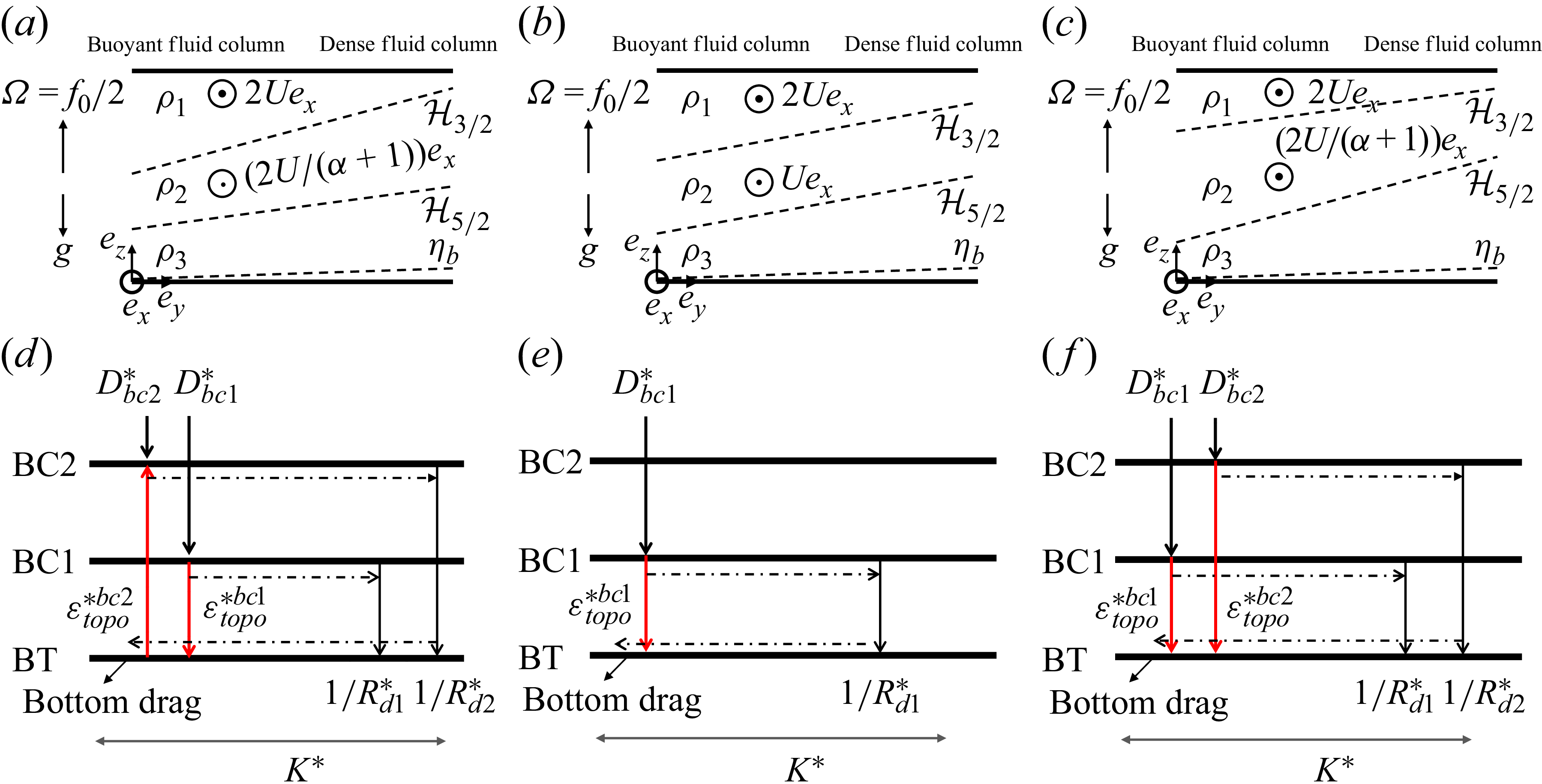
 f
 H3/2
 H5/2
 H3/2
 H5/2
 H5/2
 H3/2

 α=3
 Stopo/S5/2=0.8
 Cd∗=0.01
 α=1/3
 Rd1
 U

 Rd1
 U

 Cd∗=0.01

 Rd1
 U
 R2


 Rd1
 U
 R2

 Open access

