A versatile taxonomy of low-dimensional vortex models for unsteady aerodynamics

Darwin Darakananda; Jeff D. Eldredge

doi:10.1017/jfm.2018.792

A versatile taxonomy of low-dimensional vortex models for unsteady aerodynamics

Published online by Cambridge University Press: 12 November 2018

Darwin Darakananda and

Jeff D. Eldredge

Show author details

Darwin Darakananda: Affiliation:
Mechanical and Aerospace Engineering Department, University of California, Los Angeles, CA 90095, USA
Jeff D. Eldredge*: Affiliation:
Mechanical and Aerospace Engineering Department, University of California, Los Angeles, CA 90095, USA
*: †Email address for correspondence: jdeldre@ucla.edu

Article contents

Abstract
Introduction
Model formulation
Results
Conclusion
References

Rights & Permissions

Abstract

Inviscid vortex models have been demonstrated to capture the essential physics of massively separated flows past aerodynamic surfaces, but they become computationally expensive as coherent vortex structures are formed and the wake is developed. In this work, we present a two-dimensional vortex model in which vortex sheets represent shear layers that separate from sharp edges of the body and point vortices represent the rolled-up cores of these shear layers and the other coherent vortices in the wake. We develop a circulation transfer procedure that enables each vortex sheet to feed its circulation into a point vortex instead of rolling up. This procedure reduces the number of computational elements required to capture the dynamics of vortex formation while eliminating the spurious force that manifests when transferring circulation between vortex elements. By tuning the rate at which the vortex sheets are siphoned into the point vortices, we can adjust the balance between the model’s dimensionality and dynamical richness, enabling it to span the entire taxonomy of inviscid vortex models. This hybrid model can capture the development and subsequent shedding of the starting vortices with insignificant wall-clock time and remain sufficiently low-dimensional to simulate long-time-horizon events such as periodic bluff-body shedding. We demonstrate the viability of the method by modelling the impulsive translation of a wing at various fixed angles of attack, pitch-up manoeuvres that linearly increase the angle of attack from $0^{\circ }$ to $90^{\circ }$, and oscillatory pitching and heaving. We show that the proposed model correctly predicts the dynamics of large-scale vortical structures in the flow by comparing the distributions of vorticity and force responses from results of the proposed model with a model using only vortex sheets and, in some cases, high-fidelity viscous simulation.

JFM classification

Wakes/Jets: Separated flows Vortex Flows: Vortex dynamics Vortex Flows: Vortex shedding

Information

Type: JFM Papers
Information: Journal of Fluid Mechanics , Volume 858 , 10 January 2019, pp. 917 - 948
DOI: https://doi.org/10.1017/jfm.2018.792 [Opens in a new window]
Copyright: © 2018 Cambridge University Press

1 Introduction

Unsteady aerodynamics still holds a host of transient phenomena that we have yet to take advantage of in our aircraft. For example, several studies (Dickinson & Götz Reference Dickinson and Götz1993; Birch & Dickinson Reference Birch and Dickinson2001; Taira et al. Reference Taira, Dickson, Colonius and Dickinson2007) have shown that the lift on an impulsively translated plate is temporarily increased by the formation of a leading-edge vortex, resulting in a maximum lift 50 % greater than its steady-state value. Insects instinctively exploit this lift enhancement by moving their wings in ways that generate and control leading-edge vortices. While these transient effects are well documented in experiments and high-fidelity simulations, we still have difficulty effectively controlling them. This motivates our development of a model of the full flow physics that is simple enough for us to understand, low-dimensional enough to be used for real-time flow control, yet dynamically rich enough to capture the essential phenomena. The rich library of inviscid vortex models provides a good foundation for building such a model.

Vortex models distil flow physics into the production of simple vortex elements and the dynamics governing their motion. Each element represents a parcel of vorticity in the fluid. At high Reynolds numbers, the diffusion of vorticity is negligible compared with its inertial motion, so the evolution of the flow field can be approximated by the inviscid advection of vortex elements. In the earliest vortex models (Wagner Reference Wagner1925; Theodorsen Reference Theodorsen1935; von Kármán & Sears Reference von Kármán and Sears1938), vortex elements are only produced at the trailing edge of the wing. The elements remain fixed where they are deposited, forming a continuous planar vortex sheet behind the wing. While these simplifications allow the models to admit linearly composable analytical solutions, they limit the wing kinematics to small perturbations about low angles of attack.

To expand the range of wing kinematics, later models (Sarpkaya Reference Sarpkaya1975; Katz Reference Katz1981; Jones Reference Jones2003; Ansari, Zbikowski & Knowles Reference Ansari, Zbikowski and Knowles2006; Ramesh et al. Reference Ramesh, Gopalarathnam, Edwards, Ol and Granlund2013) release vortex elements from both edges of the wing, and allow the elements to move according to classical vortex dynamics. The increased number of elements enables these models to capture a much richer set of transient phenomena, such as the formation of leading-edge vortices and the emergence of coherent vortex structures. Unfortunately, these models no longer have analytical solutions, and flow response must be numerically computed. The interaction between vortex elements requires computing an $n$ -body problem (with $n$ being the number of elements) at every simulation time step. Even using fast summation methods (Greengard & Rokhlin Reference Greengard and Rokhlin1987) that can solve $n$ -body problems in $O(n)$ , the computational complexity of these models is at best quadratic in time, as new elements must be regularly introduced into the fluid to model vorticity production. This quadratic growth of time complexity makes these vortex models impracticable for real-time applications.

Instead of simulating vorticity production by adding new elements, another class of vortex models (Brown & Michael Reference Brown and Michael1954; Michelin & Llewellyn Smith Reference Michelin and Llewellyn Smith2009; Tchieu & Leonard Reference Tchieu and Leonard2011; Wang & Eldredge Reference Wang and Eldredge2013) feeds vorticity directly into existing vortex elements. These low-order models use a variable-strength point vortex to capture the bulk characteristics of each coherent vortex, enabling them to describe the dynamics of the leading- and trailing-edge vortices without simulating their internal structure. This simplification decouples the number of vortex elements in the fluid from the temporal resolution of the simulation. Instead of releasing elements at every time step, these models add new elements only when new coherent vortices are formed. However, in a fully viscous flow, coherent vortices precipitate from vorticity already in the fluid, via instabilities in shear layers. Thus, condensing the internal structure of vorticity-filled regions into single points removes the natural mechanism for creating new large-scale structures. While the massive reduction in element count makes these models simple to understand and enables them to run in real time, the lack of a natural vortex shedding mechanism makes them dynamically incomplete for investigating long-term flow behaviour.

In order to create a single model that satisfies all of our requirements, we combine features from several existing vortex models. Our model uses vortex sheets to represent the wing (represented here as an infinitely thin flat plate) and the free shear layers that separate from the wing’s edges. By monitoring the dynamics of the free vortex sheets, we can detect the growth of new coherent vortices in the fluid. However, as each vortex sheet is discretely represented by a large collection of vortex elements, the use of spiralling sheets to model growing coherent vortices is computationally expensive. For this purpose, then, we follow the examples of the low-order models and represent each coherent vortex with a single point vortex. The growth of these large-scale vortices can then be modelled by transferring vorticity from the tips of the vortex sheets into the point vortices.

Though this hybrid representation has been used to a limited degree in some previous studies (Pullin Reference Pullin1978; Jones Reference Jones2003; Li & Wu Reference Li and Wu2016), the approach we follow here is uniquely able to ensure that the force exerted on the plate is not spuriously affected by this transfer of circulation between a finite-length vortex sheet and its point vortex core. This approach makes use of an extended version of the impulse matching principle that was developed by Wang & Eldredge (Reference Wang and Eldredge2013). By using both vortex sheets and point vortices, we show that we can limit the number of vortex elements in our model without losing the ability to naturally create new vortex structures. While previous investigators (Sarpkaya Reference Sarpkaya1975; Chorin Reference Chorin1990; Rossi Reference Rossi1997) have also aggregated vortex elements to reduce computational cost, they focused on identifying elements that can be merged without adversely affecting the velocity field induced by these elements (without regard for the modifying presence of the body). These merging schemes naturally tend to restrict the distances between the mergeable vortex elements.

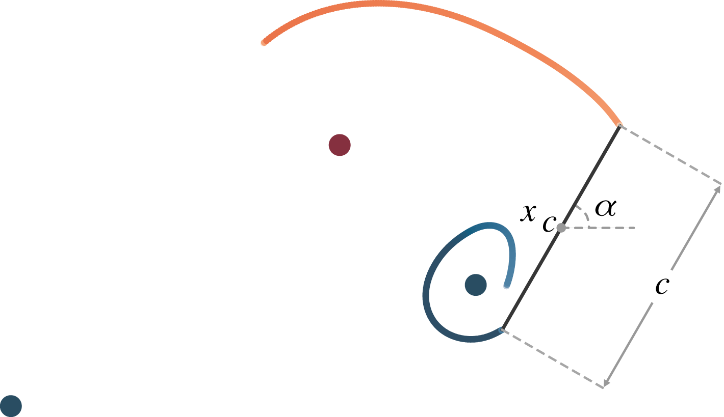
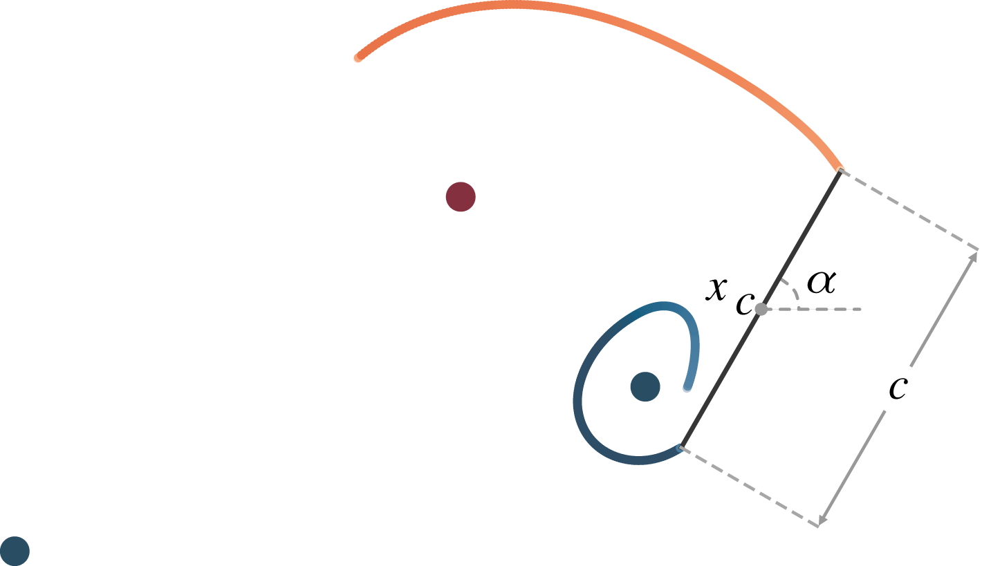
In the present work we seek to transfer circulation from the vortex sheets directly to the point vortex representing its core, as shown in figure 1. We typically do not want the tip of the vortex sheet to be near its associated point vortex in order to avoid simulating the details of vortex sheet rollup. Thus, we generally will seek to transfer circulation across larger distances than usually considered in these previous aggregation schemes. Since we ultimately are interested in the force exerted by the fluid on the plate, we will instead construct the transfer process to preserve the model’s force response rather than the moments of the vorticity field. This impulse matching approach will naturally account for the role of the body in the merging process. We describe the details of the circulation transfer process in § 2, then apply it to test problems in § 3. In the process of addressing these test problems, we will explore the convergence of the model (towards the results obtained with a pure vortex sheet) and the computational cost.

2 Model formulation

We model the ambient vorticity with three types of vortex elements:

(i) an ordered collection of point vortices, comprising a vortex sheet rooted at an edge of the wing to represent the separated shear layer at that edge (Jones Reference Jones2003; Nitsche, Taylor & Krasny Reference Nitsche, Taylor and Krasny2003; Shukla & Eldredge Reference Shukla and Eldredge2007);
(ii) an active (i.e. variable-strength) advecting discrete point vortex associated with each vortex sheet to represent its rolled-up core; and
(iii) a collection of inactive (i.e. constant-strength) advecting discrete point vortices to represent large-scale vortex structures in the wake.

The active and inactive vortex elements are referred to collectively as ‘discrete’ vortex elements in this paper, to distinguish them from the point vortices that constitute the sheet. The total number of vortex elements, including the discrete elements and the constituent point vortices of the sheet, is denoted by $N_{v}$ .

As noted by Moore (Reference Moore1979) and Krasny (Reference Krasny1986), vortex sheets are inherently unstable and will amplify errors from numerical round-off. Therefore, we regularize the interactions between all point vortices, including the active and inactive discrete vortices as well as those in the sheets, via the commonly used velocity kernel,

(2.1)

$$\begin{eqnarray}\displaystyle -\frac{\boldsymbol{x}}{2\unicode[STIX]{x03C0}(|\boldsymbol{x}|^{2}+\unicode[STIX]{x1D6FF}^{2})}, & & \displaystyle\end{eqnarray}$$

where $\unicode[STIX]{x1D6FF}$ is the so-called ‘blob radius’. The choice for the blob radius will be discussed below.

The wing is modelled as an infinitely thin flat plate of length $c$ undergoing rigid-body motion, as illustrated in figure 1. (The method introduced in this paper is not restricted to thin flat plates, but we do not address the details of applying it to other airfoil geometries.) At every time step, we add new segments of circulation to the plate end of the vortex sheets to enforce the Kutta condition – or, in certain cases described below, the leading-edge suction criterion (Ramesh et al. Reference Ramesh, Gopalarathnam, Granlund, Ol and Edwards2014) – at these edges. At the same time, we trim the number of vortex elements in our system by transferring circulation from the free end of the sheets into the active point vortices. This procedure is described in detail below.

Figure 1.

The model: $\boldsymbol{x}_{c}$ , $\unicode[STIX]{x1D6FC}$ and $c$ denote the centroid, angle of attack and chord length of the plate. Each vortex sheet has an associated point vortex that it feeds circulation into.

2.1 Effect of circulation transfer on force

Before describing the model, it is important to review the relationship between the transfer of circulation among vortex elements and the force exerted by the fluid on the plate. This force is equal and opposite to the rate of change of momentum (i.e. linear impulse) in the fluid. By transferring circulation across finite distance in a small time step, we are unavoidably effecting a spurious change of impulse – and thus, giving rise to a non-physical component of force. However, by isolating the spurious effect, we can correct for it.

Let $\boldsymbol{F}$ be the force exerted on a body as it moves through a fluid with density $\unicode[STIX]{x1D70C}$ . If $\boldsymbol{P}$ is the linear impulse of the fluid, then

(2.2)

$$\begin{eqnarray}\displaystyle \boldsymbol{F}=-\unicode[STIX]{x1D70C}\frac{\text{d}\boldsymbol{P}}{\text{d}t}. & & \displaystyle\end{eqnarray}$$

In two dimensions, the fluid impulse takes the form:

(2.3)

$$\begin{eqnarray}\displaystyle \boldsymbol{P}=\int \boldsymbol{x}\times \unicode[STIX]{x1D74E}\,\text{d}A+\oint \boldsymbol{x}\times \unicode[STIX]{x1D738}\,\text{d}l+\oint \boldsymbol{x}\times (\hat{\boldsymbol{n}}\times \boldsymbol{u}_{B})\,\text{d}l, & & \displaystyle\end{eqnarray}$$

where $\unicode[STIX]{x1D74E}$ is the vorticity in the fluid, $\unicode[STIX]{x1D738}$ is the strength of the bound vortex sheet on the body, $\hat{\boldsymbol{n}}$ is the normal vector on the body surface (directed into the fluid) and $\boldsymbol{u}_{B}$ is the velocity at the body surface. Since our wing is modelled as a plate with infinitesimal thickness, the last integral in (2.3) is zero, leaving us only the impulse from ambient vorticity and the bound vortex sheet. The bound vortex sheet is necessary to maintain the no-flow-through condition on the body surface. If we decompose the ambient vorticity field into $N_{v}$ vortex elements (including the point vortices that comprise the discretized free vortex sheets), with positions $\boldsymbol{x}_{i}$ and strengths $\unicode[STIX]{x1D71E}_{i}=\unicode[STIX]{x1D6E4}_{i}\boldsymbol{e}_{z}$ , then we can interpret the bound vortex sheet as a superposition of $N_{v}+1$ sheets, that is

(2.4)

$$\begin{eqnarray}\displaystyle \unicode[STIX]{x1D738}=\mathop{\sum }_{i=1}^{N_{v}}\unicode[STIX]{x1D738}_{i}+\unicode[STIX]{x1D738}_{B}, & & \displaystyle\end{eqnarray}$$

where each $\unicode[STIX]{x1D738}_{i}$ cancels out the body normal velocity induced by the $i$ th vortex element in the fluid, and $\unicode[STIX]{x1D738}_{B}$ enforces the normal velocity due to the body’s motion. Kelvin’s circulation theorem is globally enforced by setting the circulation of each bound sheet $\unicode[STIX]{x1D738}_{i}$ to $-\unicode[STIX]{x1D6E4}_{i}$ and the circulation of $\unicode[STIX]{x1D738}_{B}$ to zero.

We take advantage of this interpretation in (2.4) and decompose the fluid impulse into two components, $\boldsymbol{P}=\boldsymbol{P}_{A}+\boldsymbol{P}_{B}$ , where

(2.5)

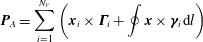$$\begin{eqnarray}\displaystyle \boldsymbol{P}_{A}=\mathop{\sum }_{i=1}^{N_{v}}\left(\boldsymbol{x}_{i}\times \unicode[STIX]{x1D71E}_{i}+\oint \boldsymbol{x}\times \unicode[STIX]{x1D738}_{i}\,\text{d}l\right) & & \displaystyle\end{eqnarray}$$

and

(2.6)

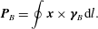$$\begin{eqnarray}\displaystyle \boldsymbol{P}_{B}=\oint \boldsymbol{x}\times \unicode[STIX]{x1D738}_{B}\,\text{d}l. & & \displaystyle\end{eqnarray}$$

Since $\boldsymbol{P}_{B}$ and its rate of change are independent of the vortex dynamics, the process of transferring circulation between vortex elements will only influence $\text{d}\boldsymbol{P}_{A}/\text{d}t$ . Let us distinguish the contributions of each vortex element to the rate of change of $\boldsymbol{P}_{A}$ . The strength distribution of each element’s associated bound vortex sheet, $\unicode[STIX]{x1D738}_{i}$ , is proportional to $\unicode[STIX]{x1D6E4}_{i}$ and a function of the associated vortex position, $\boldsymbol{x}_{i}$ . Thus, the expression for impulse due to ambient vorticity in (2.5) can be written as

(2.7)

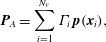$$\begin{eqnarray}\displaystyle \boldsymbol{P}_{A}=\mathop{\sum }_{i=1}^{N_{v}}\unicode[STIX]{x1D6E4}_{i}\,\boldsymbol{p}(\boldsymbol{x}_{i}), & & \displaystyle\end{eqnarray}$$

where $\boldsymbol{p}(\boldsymbol{x}_{i})$ is the impulse of a unit-strength vortex element located at $\boldsymbol{x}_{i}$ plus the impulse of its associated bound vortex sheet of strength $\unicode[STIX]{x1D738}_{i}$ (with $\unicode[STIX]{x1D6E4}_{i}$ set to unity). We then have

(2.8)

$$\begin{eqnarray}\displaystyle \frac{\text{d}\boldsymbol{P}_{A}}{\text{d}t}=\mathop{\sum }_{i=1}^{N_{v}}\left(\unicode[STIX]{x1D6E4}_{i}\frac{\text{d}\boldsymbol{p}}{\text{d}\boldsymbol{x}_{i}}\boldsymbol{\cdot }\dot{\boldsymbol{x}}_{i}+\dot{\unicode[STIX]{x1D6E4}}_{i}\,\boldsymbol{p}(\boldsymbol{x}_{i})\right). & & \displaystyle\end{eqnarray}$$

For inviscid flows, Kelvin’s circulation theorem requires circulation to be conserved within any materially transported loop, with $\dot{\unicode[STIX]{x1D6E4}}_{i}$ equal to zero. A variable-strength vortex, for which $\dot{\unicode[STIX]{x1D6E4}}_{i}\neq 0$ , serves as a simple representation of a more extensive vortex structure and its time-varying strength reflects a flux of vorticity into or out of this structure from other parts of the flow. The physical mechanism of this flux is not explicitly represented; only its effect is captured, via the transfer of circulation between vortex elements. But (2.8) shows that by violating Kelvin’s theorem, as we do here, we will introduce a spurious force that is proportional to $\dot{\unicode[STIX]{x1D6E4}}_{i}$ .

2.2 Impulse matching velocity correction

As we are intent on transferring circulation, we will offset the unwanted change to the force by modifying the velocity of a vortex element. Let us denote the vortex elements we are transferring circulation between with subscripts $s$ and $t$ (for ‘source’ and ‘target’). To conserve total circulation, we feed circulation into the target element at the same rate that we draw it from the source element, that is

(2.9)

$$\begin{eqnarray}\displaystyle \dot{\unicode[STIX]{x1D6E4}}=\dot{\unicode[STIX]{x1D6E4}}_{t}=-\dot{\unicode[STIX]{x1D6E4}}_{s}. & & \displaystyle\end{eqnarray}$$

The target element’s position is evolved according to

(2.10)

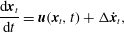$$\begin{eqnarray}\displaystyle \frac{\text{d}\boldsymbol{x}_{t}}{\text{d}t}=\boldsymbol{u}(\boldsymbol{x}_{t},t)+\unicode[STIX]{x0394}\dot{\boldsymbol{x}}_{t}, & & \displaystyle\end{eqnarray}$$

with an additional velocity, $\unicode[STIX]{x0394}\dot{\boldsymbol{x}}_{t}$ , chosen such that the spurious force arising in (2.8) from the circulation transfer is cancelled:

(2.11)

$$\begin{eqnarray}\displaystyle -\frac{1}{\unicode[STIX]{x1D70C}}\unicode[STIX]{x0394}\boldsymbol{F}=\unicode[STIX]{x1D6E4}_{t}\frac{\text{d}\boldsymbol{p}}{\text{d}\boldsymbol{x}}(\boldsymbol{x}_{t})\boldsymbol{\cdot }\unicode[STIX]{x0394}\dot{\boldsymbol{x}}_{t}+\dot{\unicode[STIX]{x1D6E4}}(\,\boldsymbol{p}(\boldsymbol{x}_{t})-\boldsymbol{p}(\boldsymbol{x}_{s}))=0. & & \displaystyle\end{eqnarray}$$

Wang & Eldredge (Reference Wang and Eldredge2013) used this approach, which they called ‘impulse matching’, to directly transfer circulation from the bound vortex sheet of the body to an active point vortex. In the present model, we will generalize the approach and use it to transfer circulation from a free vortex sheet in the fluid to an active point vortex. We defer the derivation of the velocity correction to appendix A and simply present the result below. To streamline the presentation, we will use complex coordinates where $z:=x+\text{i}y$ is the complex position in inertial coordinates, and $\tilde{z}$ is the dimensionless position in a plate-centred frame of reference,

(2.12)

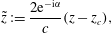$$\begin{eqnarray}\displaystyle \tilde{z}:=\frac{2\text{e}^{-\text{i}\unicode[STIX]{x1D6FC}}}{c}(z-z_{c}), & & \displaystyle\end{eqnarray}$$

where $z_{c}$ is the complex coordinate of the plate’s centroid, $c$ is the plate chord length and $\unicode[STIX]{x1D6FC}$ its angle of attack; see figure 1. The velocity correction, in inertial coordinates, can then be written as

(2.13)

$$\begin{eqnarray}\displaystyle \unicode[STIX]{x0394}{\dot{z}}_{t}=\text{i}\text{e}^{\text{i}\unicode[STIX]{x1D6FC}}\frac{c}{2}\left(\frac{(\tilde{p}_{s}-\tilde{p}_{t})(\unicode[STIX]{x1D6FD}^{\star }+1)+(\tilde{p}_{s}^{\star }-\tilde{p}_{t}^{\star })(\unicode[STIX]{x1D6FD}^{\star }-1)}{\unicode[STIX]{x1D6FD}+\unicode[STIX]{x1D6FD}^{\star }}\right)\frac{\dot{\unicode[STIX]{x1D6E4}}}{\unicode[STIX]{x1D6E4}_{t}}, & & \displaystyle\end{eqnarray}$$

where $(~)^{\star }$ denotes complex conjugation, and for $i$ either $s$ (source) or $t$ (target), the unit impulse is

(2.14)

$$\begin{eqnarray}\displaystyle \tilde{p}_{i}:=\text{Im}\{\tilde{z}_{i}\}-\text{i}\,\text{Re}\{\sqrt{\tilde{z}_{i}-1}\,\sqrt{\tilde{z}_{i}+1}\} & & \displaystyle\end{eqnarray}$$

and the gradient of the target’s impulse with respect to its position is

(2.15)

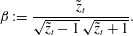$$\begin{eqnarray}\displaystyle \unicode[STIX]{x1D6FD}:=\frac{\tilde{z}_{t}}{\sqrt{\tilde{z}_{t}-1}\,\sqrt{\tilde{z}_{t}+1}}. & & \displaystyle\end{eqnarray}$$

It is important to note that the impulse matching model of Wang & Eldredge (Reference Wang and Eldredge2013) – with only variable-strength vortices and no free vortex sheets – represents a special case of the principle used here. The ‘source’ in such a case is the bound vortex sheet of the plate rather than a vortex element in the fluid, and the modified velocity of the target vortex is given by (2.13) with $\tilde{p}_{s}$ set to zero.

2.3 Circulation transfer rate

The circulation transfer process can be thought of as a real-time model order reduction process: many degrees of freedom of the constituent vortex elements at the free end of the vortex sheet are continuously eliminated in favour of the three degrees of freedom of a single variable-strength point vortex. The rate of model order reduction, controlled by the circulation transfer rate, $\dot{\unicode[STIX]{x1D6E4}}$ , is at the discretion of the user. At its other end, the sheet is rooted at the edge of the plate and fed circulation at a rate dictated by the Kutta condition. A small $\dot{\unicode[STIX]{x1D6E4}}$ magnitude may not be able to remove circulation from the sheet as fast as new circulation is introduced into it from the edge, so the sheet will tend to grow in length. However, a choice of $\dot{\unicode[STIX]{x1D6E4}}$ that exceeds this rate at the edge might change the vorticity distribution so drastically that the new reduced-order model might not preserve the essential dynamics of the original system. For example, it might eliminate the natural instability in the sheet from which new vortex structures emerge. It would seem natural to simply choose $\dot{\unicode[STIX]{x1D6E4}}$ equal to the rate of circulation introduced at the edge. But the circulation distribution at the tip of the sheet represents a historical – and generally different – value of this rate, and the distribution is further modified by the progressive effect of convective stretching. We have found that setting the transfer rate equal to the instantaneous rate at the plate edge leads to poor results.

In order to form a different strategy for choosing the transfer rate, we consider a circulation transfer that takes place over the time interval $[t_{0},\,t_{0}+\unicode[STIX]{x0394}t]$ , and, in particular, the differences between two versions of the model that are identical at time $t_{0}$ : one version in which the model is reduced in the subsequent time step – i.e. in which the circulation is transferred – and another version in which the circulation is not transferred. The velocity correction (2.13) can only guarantee that the force predicted by the reduced model is equal to that in the unreduced model at time $t_{0}$ . Since circulation transfer is not a lossless reduction of order, the small differences that emerge between the two models during the ensuing time step $\unicode[STIX]{x0394}t$ means that, in general, the forces that they predict at time $t_{0}+\unicode[STIX]{x0394}t$ will be different. We can pick $\dot{\unicode[STIX]{x1D6E4}}$ so that the difference between the predicted linear impulses in these models after $\unicode[STIX]{x0394}t$ is below an error threshold, denoted as $\unicode[STIX]{x1D716}_{F}$ .

In practice, our vortex sheets are represented as ordered collections of regularized point vortices and our model is evolved forward in time with discrete time marching. The strength of each of these vortex elements of the sheet is proportional to the time step size, since each such element is formed from the circulation flux from the plate’s edge over some previous time step. The transfer of circulation from the sheet into the target point vortex over time step $\unicode[STIX]{x0394}t$ comprises an elimination of some finite number of sheet elements from the edge of the sheet. So at every time step, we first compute the impulse that the model will predict at the end of the step if no circulation transfer occurs. We transfer circulation from as many of the regularized point vortices as we can into the active point vortex (thereby eliminating these vortices from the sheet), stopping only when the accumulated difference in predicted linear impulse exceeds the threshold $\unicode[STIX]{x1D716}_{F}$ . Since this error accumulation occurs over the time step, the threshold is set proportional to the time step size, $\unicode[STIX]{x1D716}_{F}=B_{F}\unicode[STIX]{x0394}t$ , so that the results are insensitive to the choice of $\unicode[STIX]{x0394}t$ . The proportionality constant $B_{F}$ represents the tolerance for force discrepancy in the reduced model.

There are instances when even transferring circulation from a single element from the sheet results in a large error in the predicted force. We treat this as an indication that the tip of the vortex sheet and the active point vortex have become dynamically distinct, suggesting the creation of a new vortex core. At this point, we can freeze the strength of the active point vortex (making it an inactive point vortex), and convert the tip of the vortex sheet into the new active point vortex. However, a large number of new active point vortices may be released in quick succession when small instabilities form near the tip of the vortex sheet. In order to make the method more robust to these instabilities, we require a minimum time interval between the release of new active point vortices, which we will refer to as $T_{min}$ .

Figure 2.

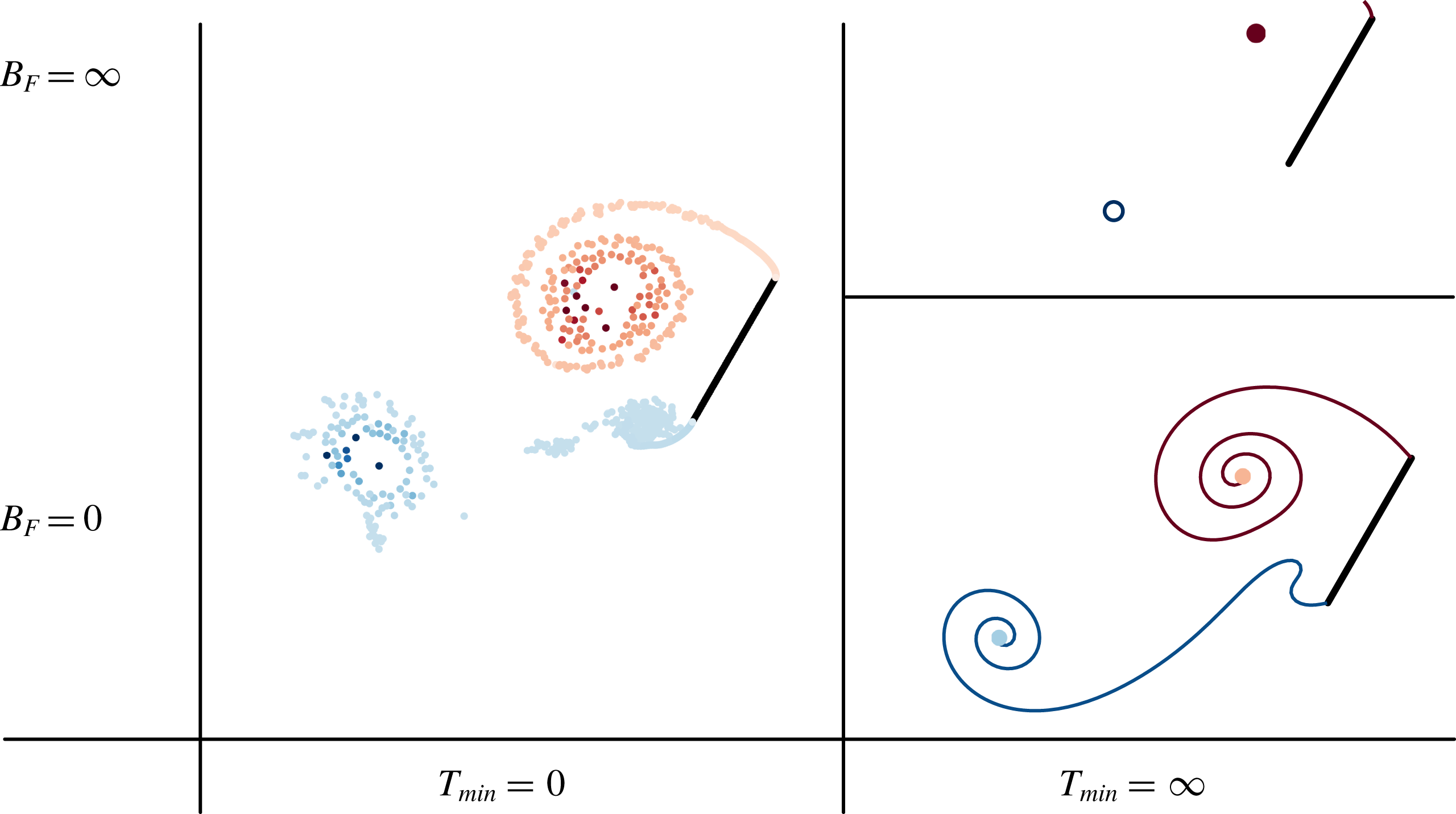
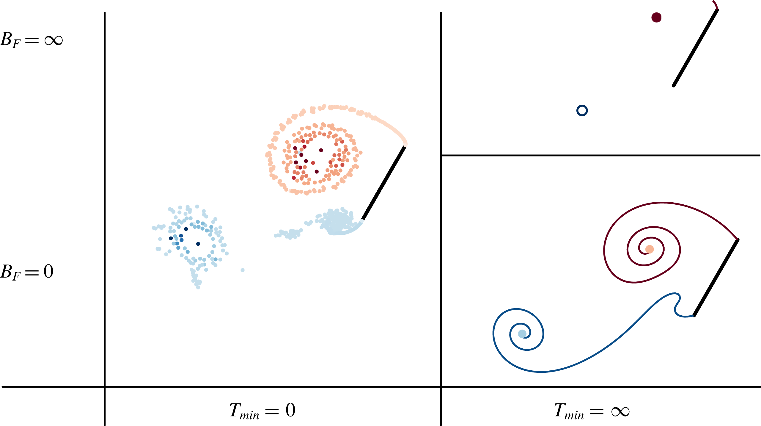
Taxonomy of vortex element models. Comparison of the vorticity distribution predicted by the hybrid model at limiting values of the tolerance for force error, $B_{F}$ , and the minimum vortex release interval, $T_{min}$ .

The independent selection of $B_{F}$ and $T_{min}$ leads to the complete taxonomy of inviscid vortex models, as depicted in figure 2. Suppose we set $T_{min}=0$ . This means that the sheet’s last vortex element is converted into a distinct point vortex at every time step, regardless of the value of $B_{F}$ , which leads to a traditional discrete vortex element model (Sarpkaya Reference Sarpkaya1975; Katz Reference Katz1981; Xia & Mohseni Reference Xia and Mohseni2013). Alternatively, if we set $B_{F}=0$ and $T_{min}=\infty$ , then we will still never transfer circulation to the active point vortex, but also, no new active point vortices will ever be created, leaving us essentially with a vortex sheet model (Jones Reference Jones2003; Shukla & Eldredge Reference Shukla and Eldredge2007; Alben & Shelley Reference Alben and Shelley2008). (We still initiate the model with discrete elements at the end of each sheet, as depicted in the illustration, but these do not gather further strength when $B_{F}=0$ .) If we instead make $B_{F}=\infty$ and $T_{min}=\infty$ , then any circulation shed from the plate to the sheet through the Kutta condition is immediately absorbed into the active point vortex, giving us a slightly modified version of the impulse matching model of Wang & Eldredge (Reference Wang and Eldredge2013). And if we substitute the modified velocity of the vortex derived here by impulse matching, we can obtain the variable-strength vortex model used by previous researchers, based on the Brown–Michael model (Brown & Michael Reference Brown and Michael1954; Michelin & Llewellyn Smith Reference Michelin and Llewellyn Smith2009). This qualitative description, and the associated convergence of the model to the limits, is explored further in § 3.1. Intermediate choices of $B_{F}$ and $T_{min}$ generate a spectrum of models between these extremes, as we will see in the examples below.

Once we have picked values of $B_{F}$ and $T_{min}$ , then we perform the following procedure in every time step:

(i) For every point vortex comprising the vortex sheet, we compute and store the velocity correction it will contribute to the active point vortex if we transfer all of its circulation to that vortex.
(ii) Advect all vortex elements forward in time (with their unmodified velocities) and compute each vortex’s individual impulse. To achieve this step, the bound vortex sheet strength is calculated and Biot–Savart interactions between elements are computed.
(iii) Starting from the free end of the vortex sheet, we attempt to transfer circulation. Suppose we have already transferred circulation from $n_{v}$ point vortices from the vortex sheet, and we are attempting to transfer circulation from the $(n_{v}+1)$ th one. Then:
1. (a) We compute the impulse and modified position of the active point vortex with the accumulated circulation and velocity correction from the $(n_{v}+1)$ point vortices.
2. (b) If the difference between this impulse and that from the $(n_{v}+1)$ point vortices is less than $\unicode[STIX]{x1D716}_{F}=B_{F}\unicode[STIX]{x0394}t$ , then we transfer the circulation of this vortex (and eliminate the vortex from the sheet), and return to step ( $a$ ) and proceed to the next vortex in the sheet.
(iv) If $n_{v}>0$ , or the time since we last created a new point vortex is less than $T_{min}$ , then we continue to step (v). Otherwise, we convert the current active point vortex into an inactive one, and the tip of the vortex sheet into the new active point vortex.
(v) Apply Fourier filtering (described below) to the vortex sheet to redistribute the point vortices evenly along the sheet and remove small-scale instabilities.
(vi) Add a new vortex sheet segment at the root of each sheet to enforce the Kutta condition. The bound vortex sheet strength is recalculated for this step.

2.4 Regularization and Fourier filtering

The blob radius, $\unicode[STIX]{x1D6FF}$ , for all cases of the proposed hybrid sheet–vortex method in this study is assigned values in the range $0.01c$ – $0.05c$ , somewhat smaller than in previous studies of pure vortex sheets, where it has often been set to $0.1c$ (Krasny & Nitsche Reference Krasny and Nitsche2002; Jones Reference Jones2003; Shukla & Eldredge Reference Shukla and Eldredge2007). We have found that these smaller values are necessary to ensure robust behaviour of the sheet/active vortex system, particularly at the leading edge at small or modest angles of attack soon after the plate is set in motion. However, this smaller $\unicode[STIX]{x1D6FF}$ has the consequence of weakening the regularization’s suppression of instabilities triggered in the sheet at small length scales. Therefore, to strengthen this suppression, we apply a Fourier filtering technique along the length of each vortex sheet at every time step. In this procedure, the irregularly spaced point vortices that comprise the sheet are resampled – using linear interpolation – by a new set of point vortices distributed uniformly in arclength with spacing $3U\unicode[STIX]{x0394}t$ , where $U$ is the characteristic velocity scale and $\unicode[STIX]{x0394}t$ the time step size. (In all cases reported in this paper, the time step size has been set to $\unicode[STIX]{x0394}t=0.01c/U$ , where $U$ is a characteristic velocity – generally, the translation speed of the plate.) The filter acts on the positions of these uniformly distributed vortex elements, removing all Fourier components whose wavelength is below a certain cutoff, generally chosen to be $0.06c$ (and thus slightly larger than $\unicode[STIX]{x1D6FF}$ ).

It should be noted that such Fourier filtering would tend to artificially disrupt the natural development of vortex structures by suppressing the formation of spirals below the filter cutoff (Krasny Reference Krasny1986). However, in all cases in which this filtering is used here, the core of the vortex structure is replaced by an active point vortex; only large spirals will form before they are siphoned into the active vortex, and these spirals will always have length scales above the cutoff and will form unabated. It is important to note that, for the reference cases in this study involving only a vortex sheet, we do not use this filtering procedure; rather, we set $\unicode[STIX]{x1D6FF}=0.1c$ and, to maintain good resolution, resample the sheets onto a new set of point vortices at every step, uniformly spaced in arclength with $2U\unicode[STIX]{x0394}t$ so that even the smallest spirals are well resolved. This is only slightly less efficient than the use of judicious point insertion favoured by other researchers (Krasny & Nitsche Reference Krasny and Nitsche2002; Jones Reference Jones2003; Shukla & Eldredge Reference Shukla and Eldredge2007).

2.5 Computational cost

Figure 3.

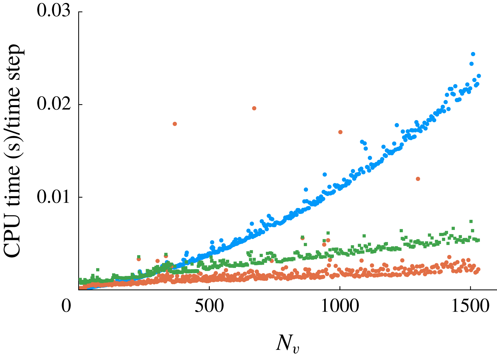
CPU time required in each time step versus the number of total vortex elements in the problem: for velocity induction and advection (●, blue), Kutta condition enforcement (▪, green), and circulation transfer procedures and sheet filtering (●, red-brown). Results generated from the simulation of an impulsively started plate at $45^{\circ }$ angle of attack.

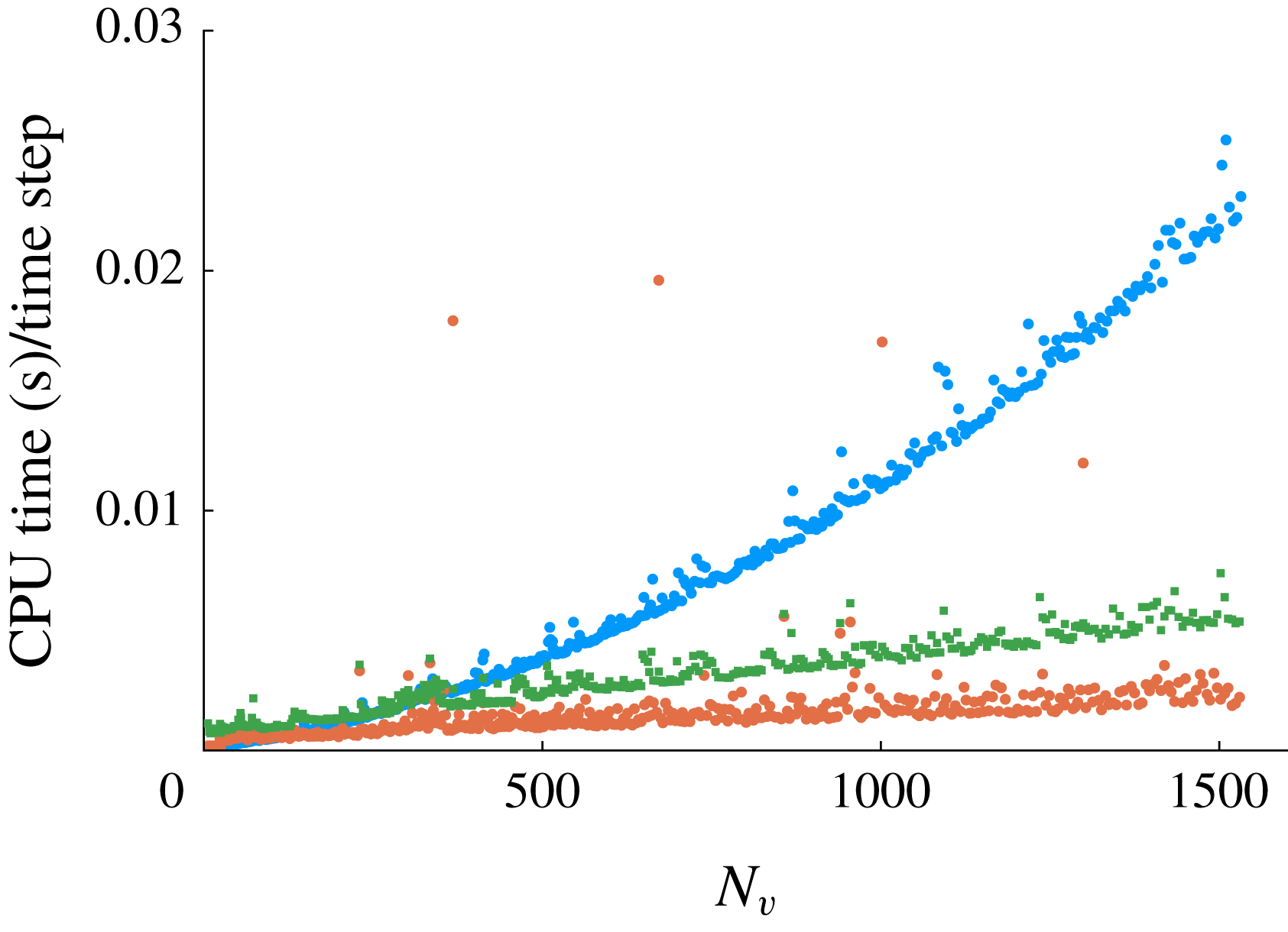
Figure 3 depicts the manner in which these various components of the algorithm contribute to the computational time in each time step. Though these results correspond to a specific case (impulsive start at $45^{\circ }$ angle of attack), they are closely representative of all cases in this paper. Step (ii) of the algorithm, consisting of Biot–Savart interactions between vortex elements and with the bound vortex sheet on the plate, scales quadratically with the number of elements. (We do not utilize a fast multipole method in this paper to accelerate such calculations.) All of the other steps – the circulation transfer procedure, the sheet filtering and the enforcement of the Kutta condition – scale linearly with the number of elements. In fact, the circulation transfer’s actual cost is attributable to the calculation of the modified velocity in (2.13). This involves only a limited number of elements at the end of the sheet (dictated by $\unicode[STIX]{x1D716}_{F}$ ), and is thus independent of the total number of elements in the sheet. The computational time we have reported here is somewhat inflated as it also includes the calculation of linear impulse for all elements of the sheet (for the calculation of fluid dynamic force) and the sheet filtering.

The total computation time of a simulation in which a large number of vortex elements is generated, such as in traditional vortex sheet and discrete vortex element models, is controlled primarily by the quadratic scaling of step (ii). However, as we will see in § 3, the hybrid method generally maintains fewer than $100$ elements, so that the other steps in the method are of comparable cost, and the overall cost per step is kept in check. The total expense of transferring circulation from the sheet into an active point vortex and of applying the filtering procedure to ensure a well-behaved sheet is minor compared to the computational savings achieved by preventing the number of elements from growing indefinitely.

3 Results

In this section, we use the proposed method to model three canonical motions: first, the impulsive translation of a plate at high angles of attack; then, a pitch-up manoeuvre; and finally, oscillatory pitching and heaving. In each, we will compare the results predicted by the new hybrid model with those from a full vortex sheet model, which we regard as the ideal for an inviscid model. In each case, time is reported in convective units, $t^{\ast }:=tU/c$ , where $U$ is the translation speed of the plate. From here on, we will report the minimum active vortex release interval, $T_{min}$ , in these units and denote it as $T_{min}^{\ast }$ . All of the results reported in this paper use a time step size $\unicode[STIX]{x0394}t^{\ast }=0.01$ and, unless otherwise reported, a threshold for force discrepancy, $B_{F}/(\unicode[STIX]{x1D70C}U^{2}c)=0.1$ .

In the first two cases, we also compare the model with high-fidelity Navier–Stokes simulations, obtained with the immersed boundary projection method developed by Taira & Colonius (Reference Taira and Colonius2007). It should be emphasized that we do not expect that the proposed inviscid model will lead to better agreement with finite-Reynolds-number results than has been achieved with previous inviscid models. As is well known, some aspects of these flows are essentially viscous and cannot be captured with a strictly inviscid approach. The high-fidelity viscous results are provided only for reference.

3.1 Impulsive translation at fixed angle of attack

3.1.1 Translation at $45^{\circ }$ angle of attack

Figure 4.

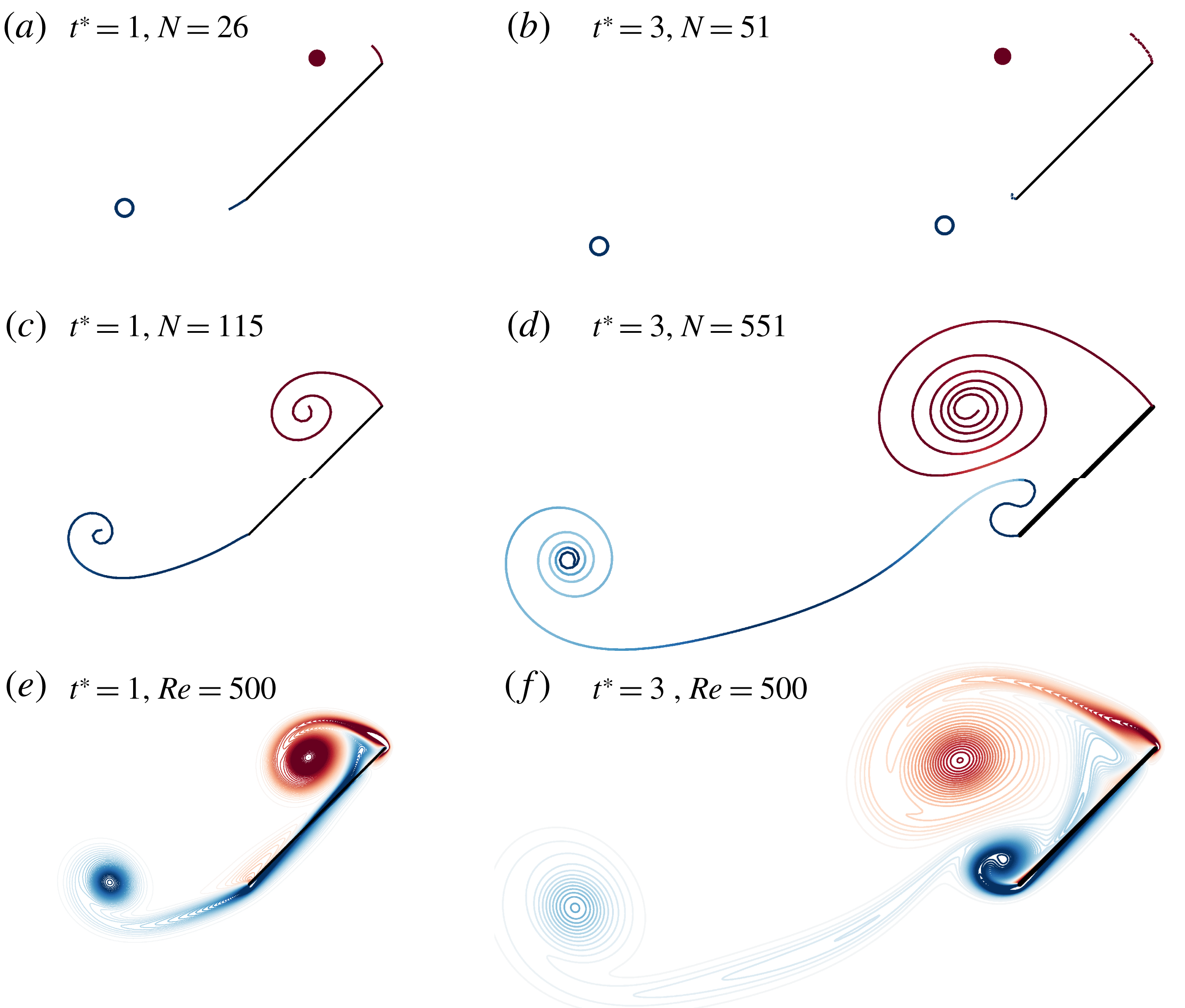
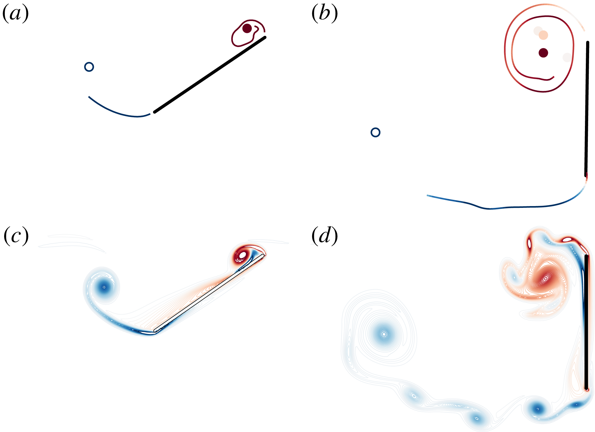
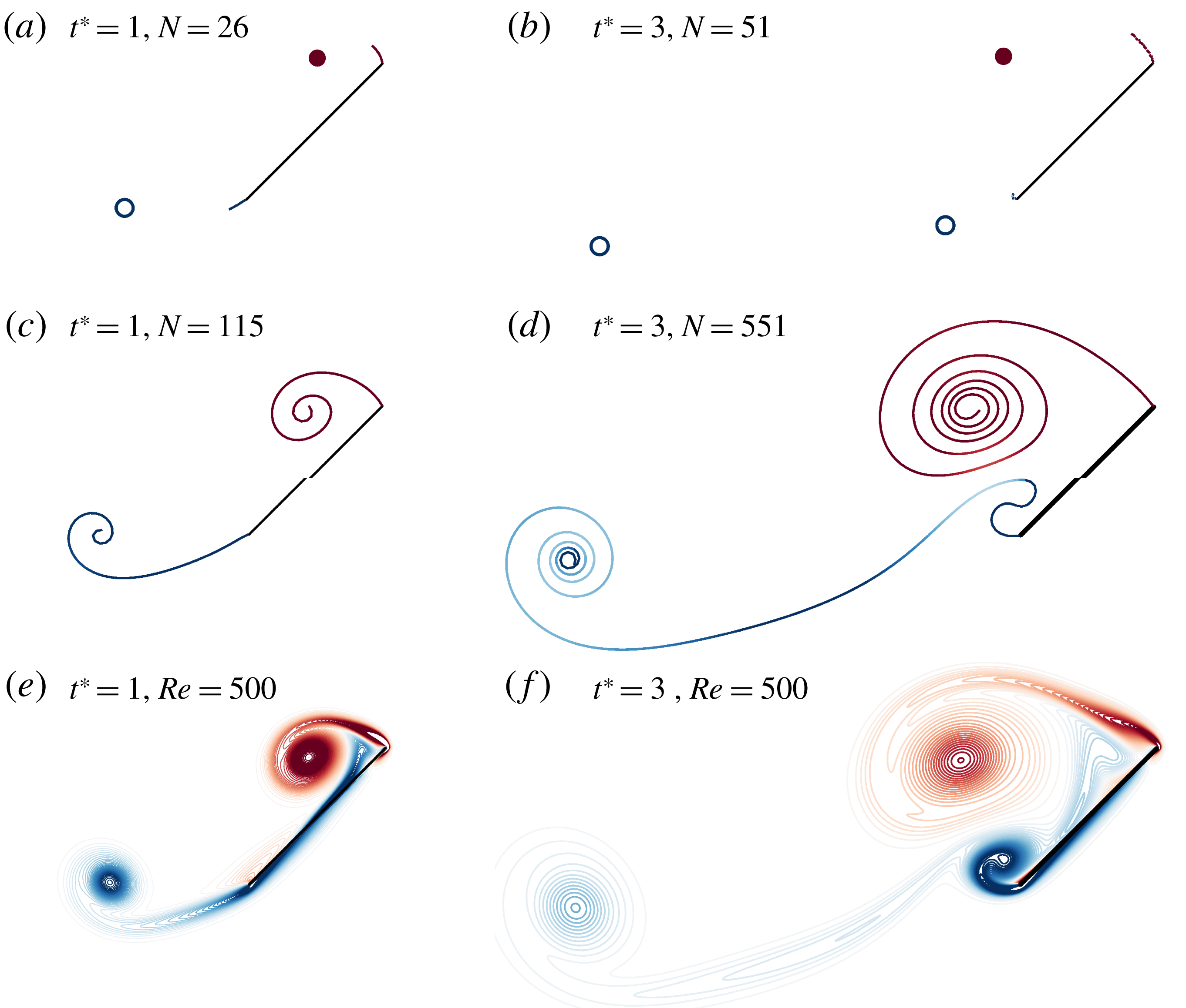
Comparison of the vorticity distribution predicted for a flat plate moved impulsively at $45^{\circ }$ after one (a,c,e) and three (b,d,f) chord lengths of travel between the new hybrid model with $T_{min}^{\ast }=0.2$ (a,b), a full vortex sheet model (c,d) and a high-fidelity simulation at $Re=500$ (e,f). The positions of the positive- and negative-strength point vortices are shown with filled and unfilled circles, respectively, and $N$ denotes the total number of vortex elements (including those in the vortex sheets).

Figure 5.

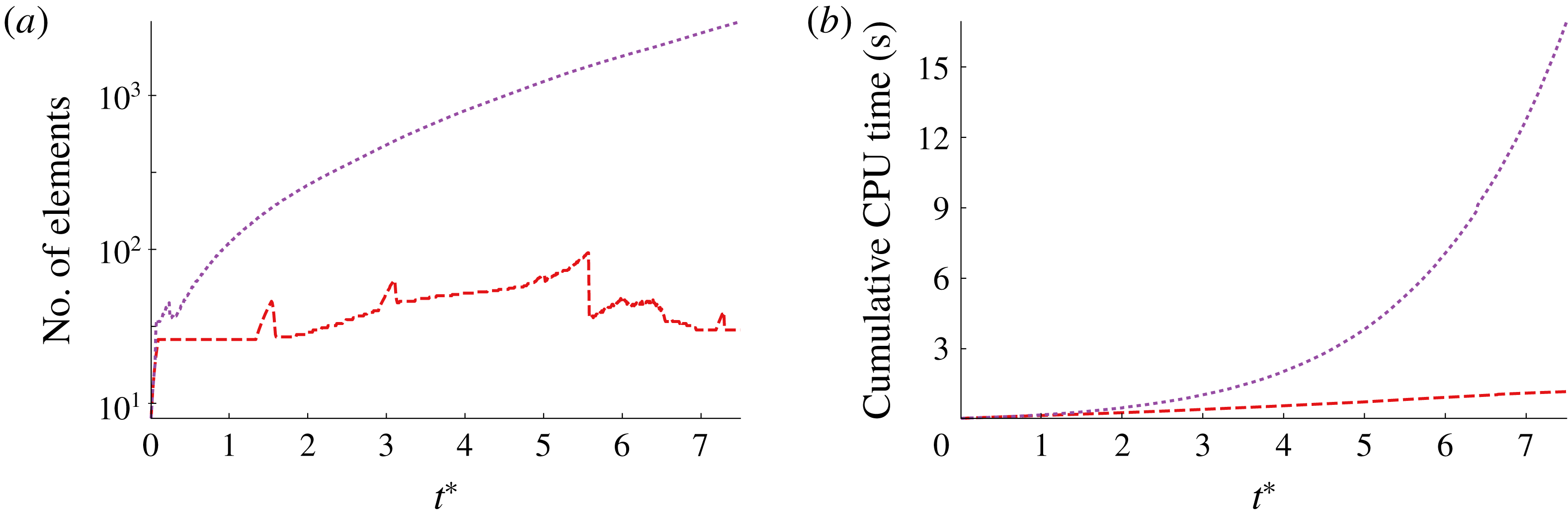
Number of vortex elements (a) and cumulative CPU time (b) of the hybrid model with $T_{min}^{\ast }=0.2$ (– –) and the vortex sheet model (- - - -), for impulsive translation at $\unicode[STIX]{x1D6FC}=45^{\circ }$ .

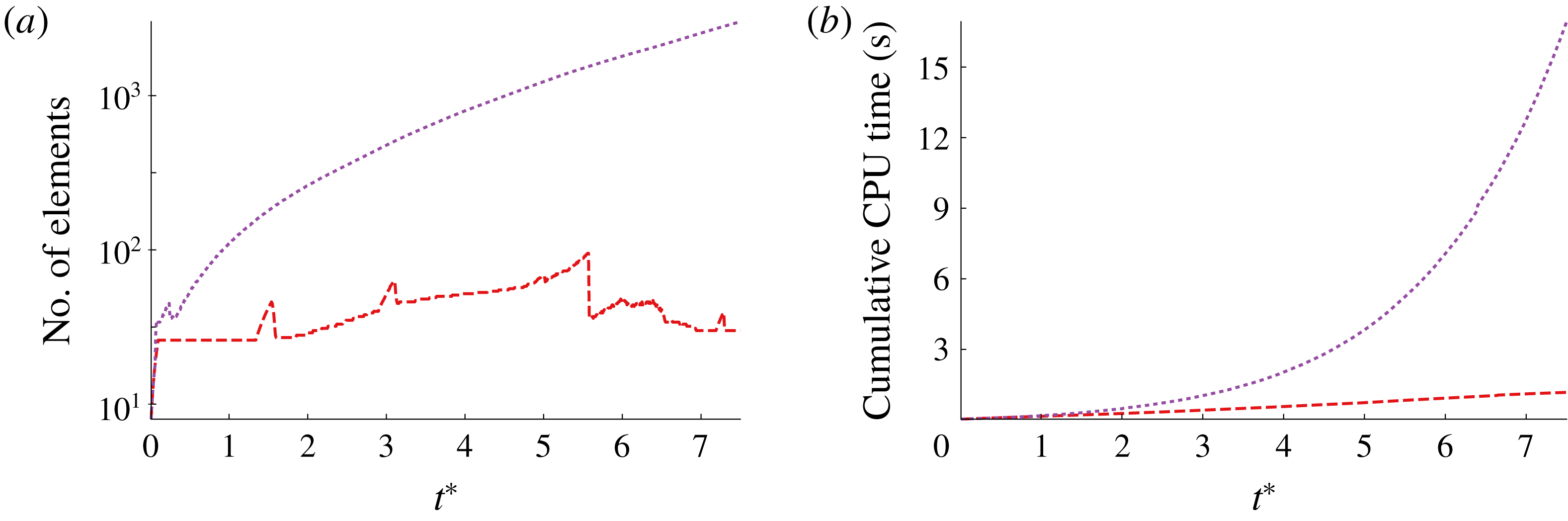
We start by considering the case at $45^{\circ }$ angle of attack. In figure 4, we compare the vorticity distribution predicted by the new hybrid model, a vortex sheet model and a $Re=500$ high-fidelity Navier–Stokes simulation after one and three convective times. The hybrid model results presented in figure 4 uses a minimum vortex release interval of $T_{min}^{\ast }=0.2$ . We see that the hybrid model captures the same large-scale vortex structures as the vortex sheet model while using an order-of-magnitude fewer computational elements. The number of vortex elements and the corresponding CPU time required to achieve these results of the hybrid model and full vortex sheet are depicted in figure 5. It is clear that the hybrid model maintains a modest number of vortex elements, while the sheet’s number of elements grows indefinitely. The computational costs of the two methods reflect these differences: the cost of the vortex sheet model grows rapidly, requiring 0.72 s to achieve $t^{\ast }=2.5$ , 3.8 s to reach $t^{\ast }=5$ and 16.9 s to get to $t^{\ast }=7.5$ . In contrast, the hybrid method requires 0.34 s, 0.73 s and 1.2 s, respectively, to reach these milestones. These performance differences are expected from the results of figure 3, since the CPU time per step scales quadratically for large element populations. Indeed, all of the cases that follow in this paper exhibit similar differences in computational performance between the full vortex sheet model and the hybrid model; though we omit the required CPU time in some cases, we report the number of computational elements for each model, and the computational cost follows accordingly.

Figure 6.

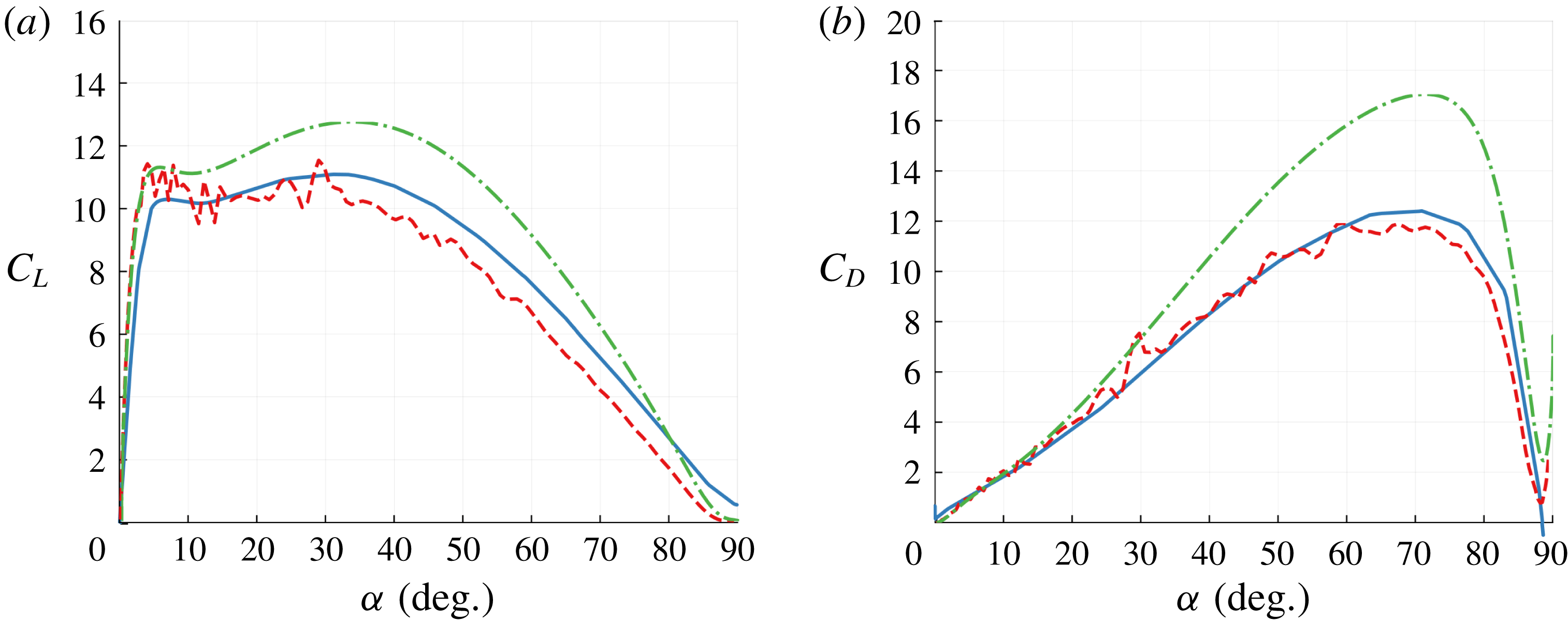
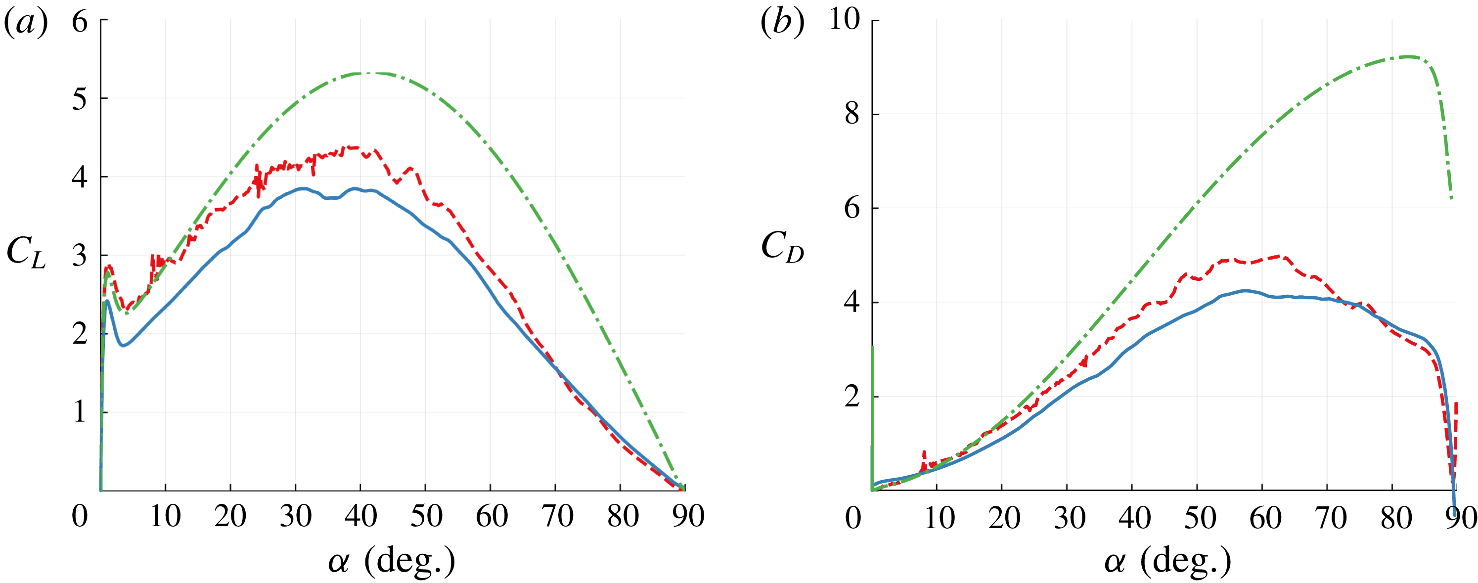
Early-time lift (a) and drag (b) coefficients for impulsive translation at $\unicode[STIX]{x1D6FC}=45^{\circ }$ predicted by the hybrid model with $T_{min}^{\ast }=0.2$ (– –), the vortex sheet model (- - - -), the Wang & Eldredge model (– ⋅ – ⋅) and high-fidelity simulation at $Re=500$ (——).

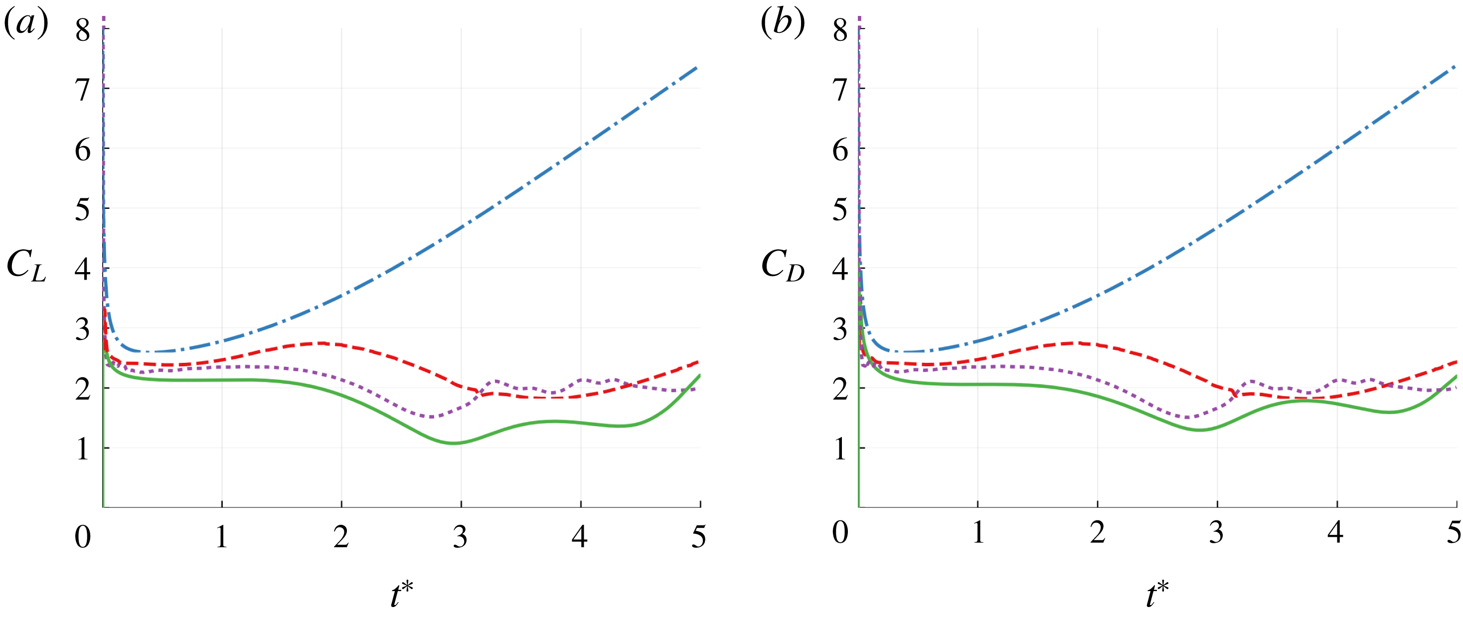
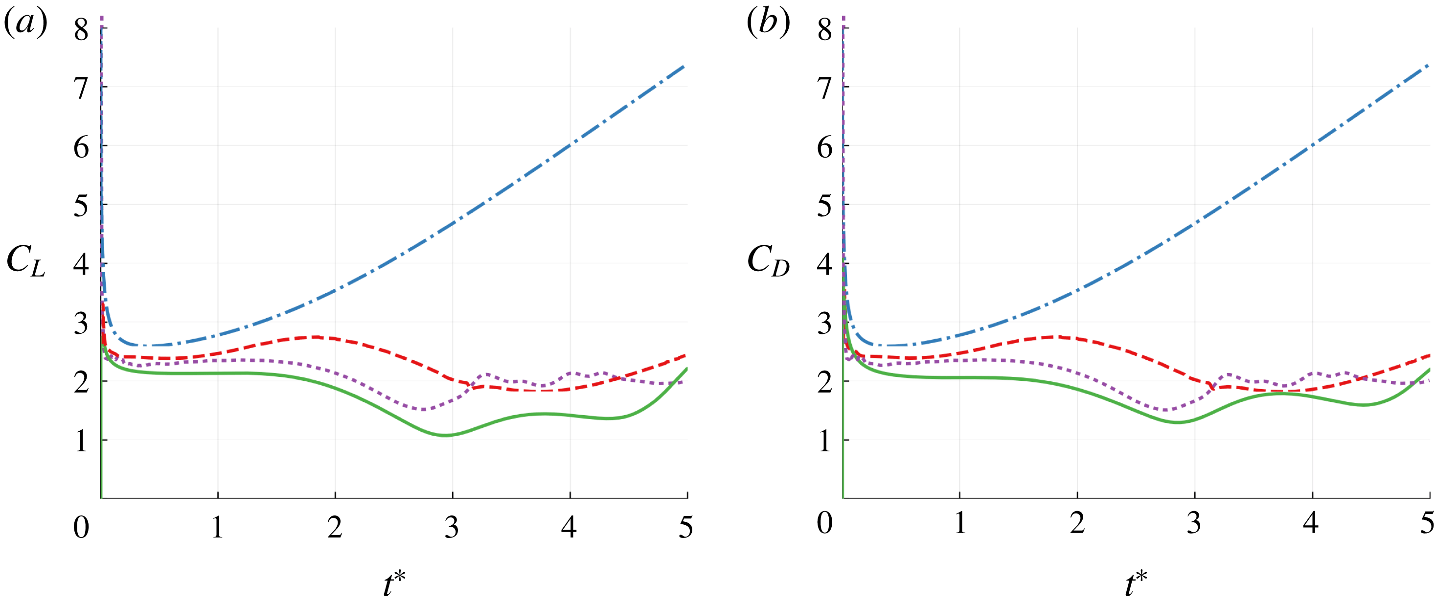
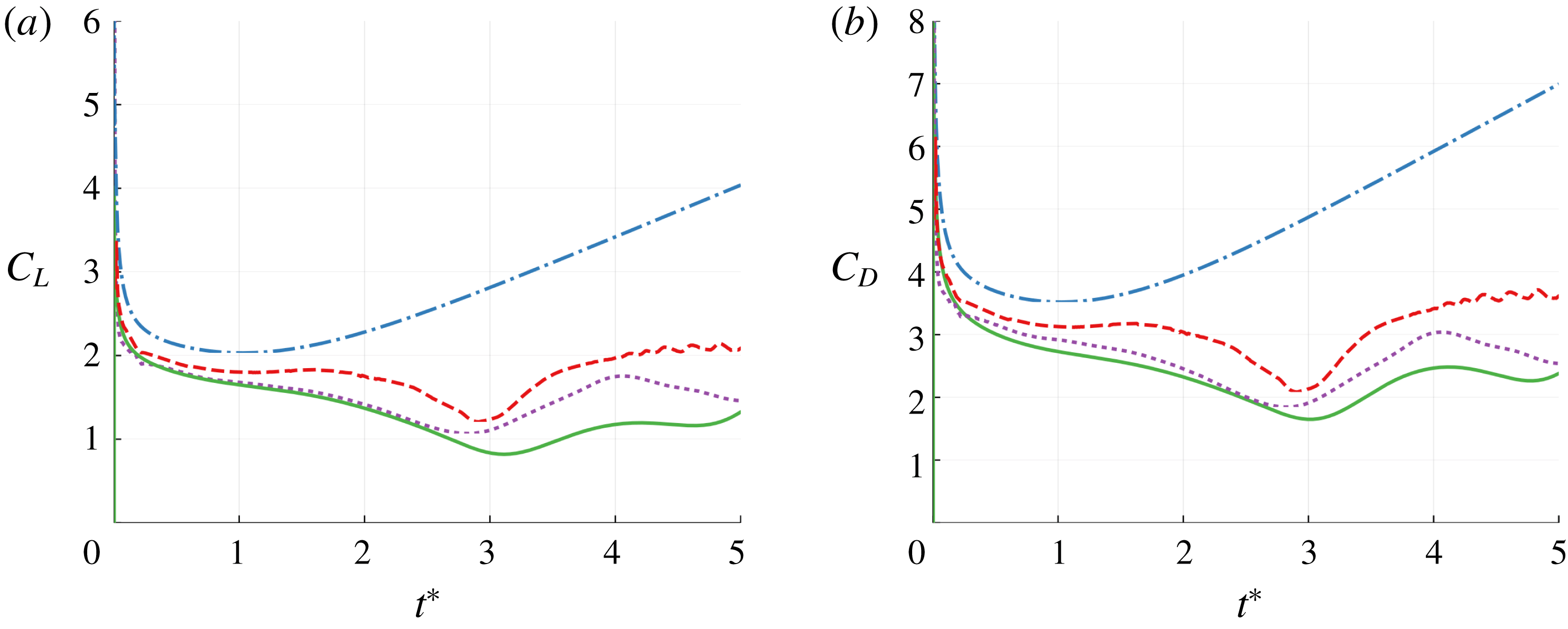
In figure 6, where we compare the lift and drag coefficients predicted by the hybrid model, the Wang & Eldredge (Reference Wang and Eldredge2013) model (i.e. only two variable-strength point vortices and no sheets), the full vortex sheet results and high-fidelity simulation results, we see that it is important that we do not completely eliminate the vortex sheets. The sheets enable the model to naturally capture the formation of new coherent vortices, which then triggers large-scale vortex shedding. This mechanism allows the hybrid model to give a more accurate force prediction than existing variable-strength point vortex models. The hybrid model is significantly more computationally efficient than the full inviscid vortex sheet model and high-fidelity viscous simulation, while generally preserving the essential dynamics of the flow and its resulting force.

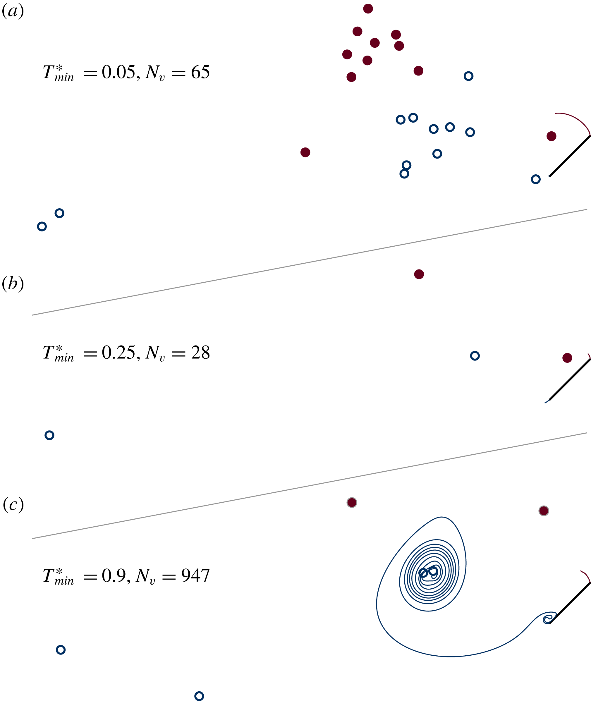
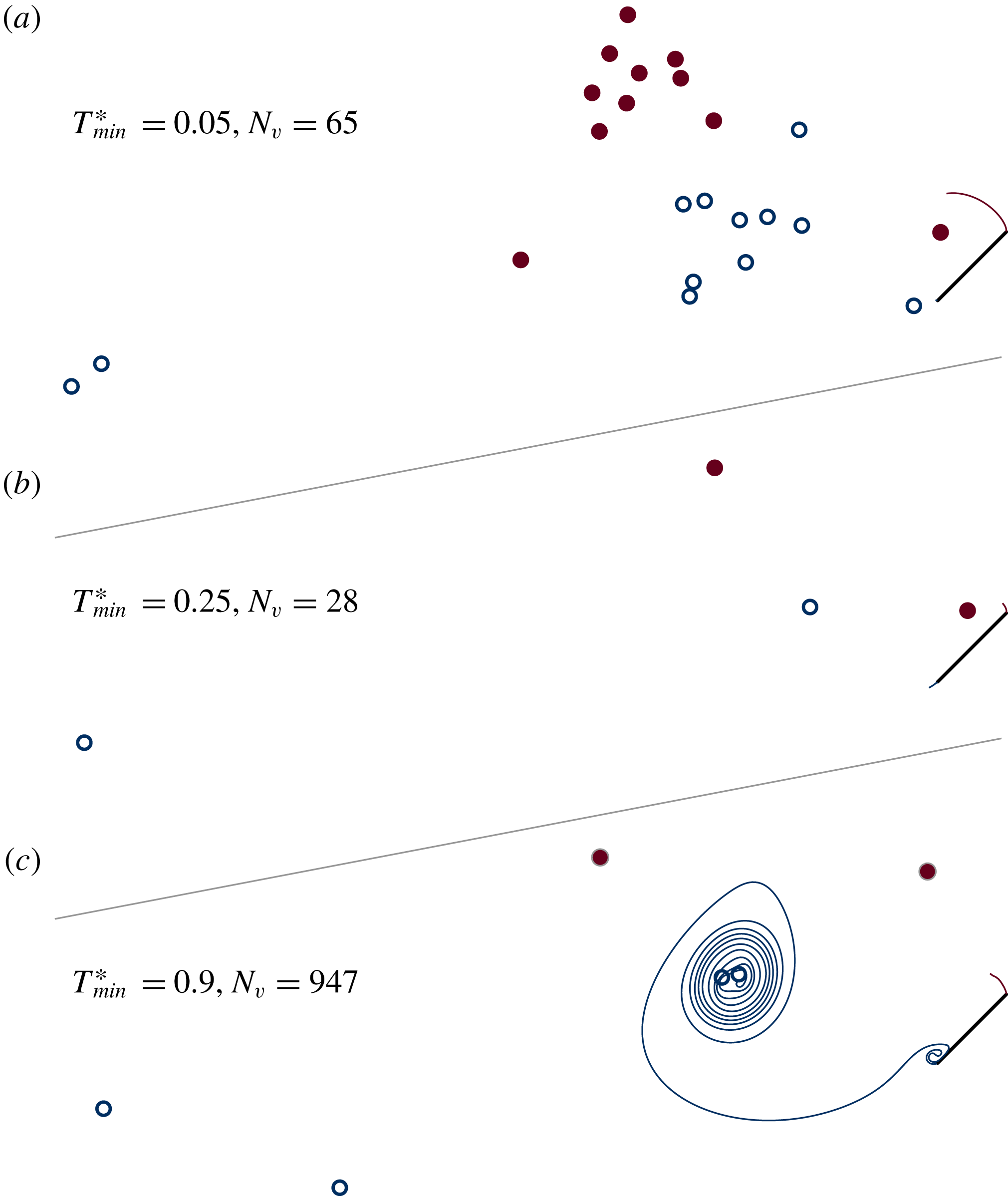
We show the effects of changing the minimum vortex release interval in figures 7–9. We see in figure 7 that a small $T_{min}^{\ast }$ gives results that are similar to those from discrete vortex element models – we tolerate more frequent initiation of new active elements, and thus create a larger population of inactive elements whose role as active elements has completed. As we increase $T_{min}^{\ast }$ , more circulation is fed into each active point vortex, so we decrease the total number of vortex elements in the model. However, very large values of $T_{min}^{\ast }$ tend to result in longer vortex sheets, which significantly increases the number of overall computational elements. 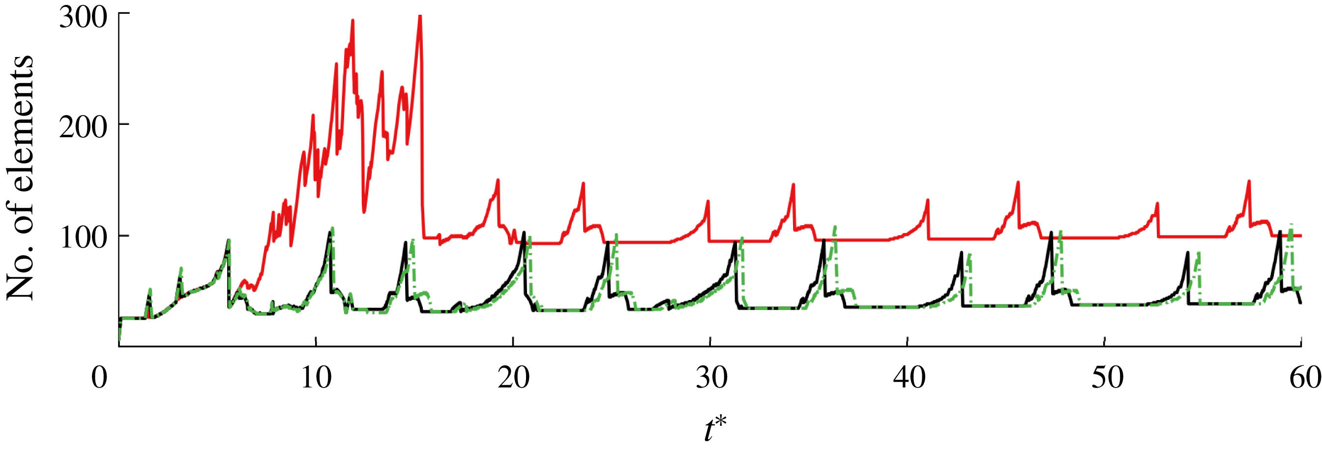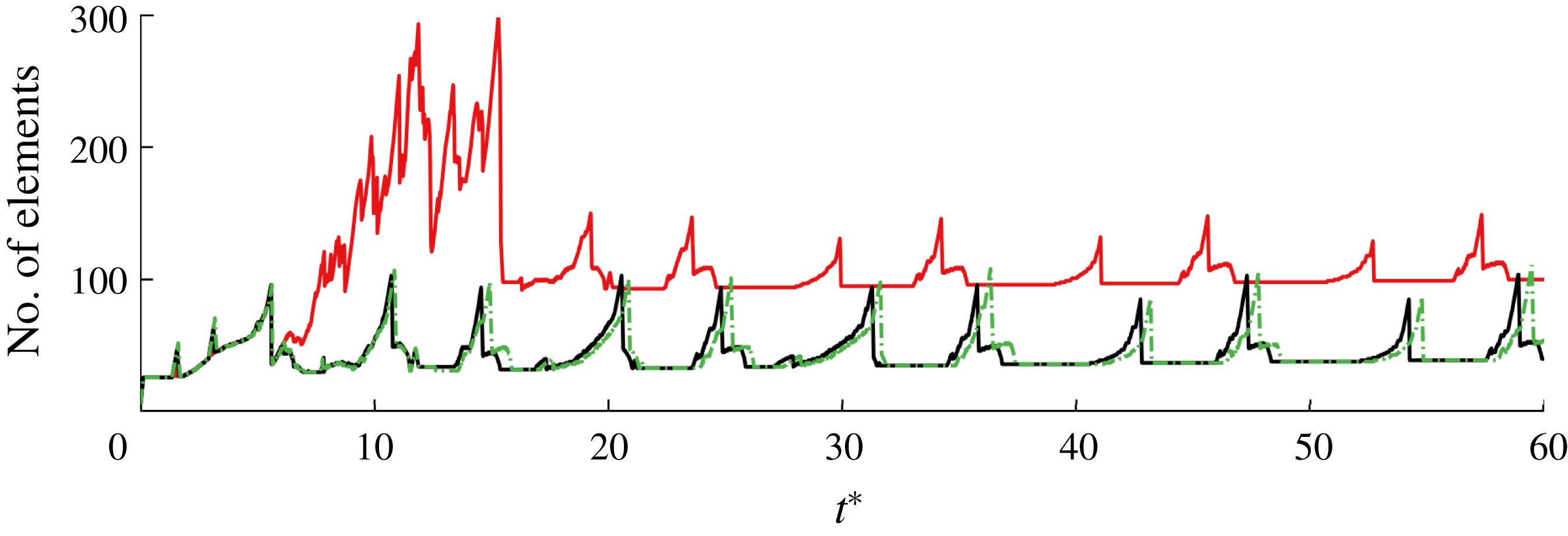In figure 8, we show how different values of $T_{min}^{\ast }$ affect the number of vortex elements used in the model over time. While the sharp increase in element count corresponds to the lengthening and growth for the vortex sheets, the sharp drops correspond to the growth of active point vortices as they consume the sheets. As long as $T_{min}^{\ast }$ is small enough to prevent the vortex sheet from growing faster than its active point vortex can absorb it, we can keep the element count low enough to simulate flows over extended periods in real time. The choices of $T_{min}^{\ast }$ and $B_{F}$ will be explored further in the next case.

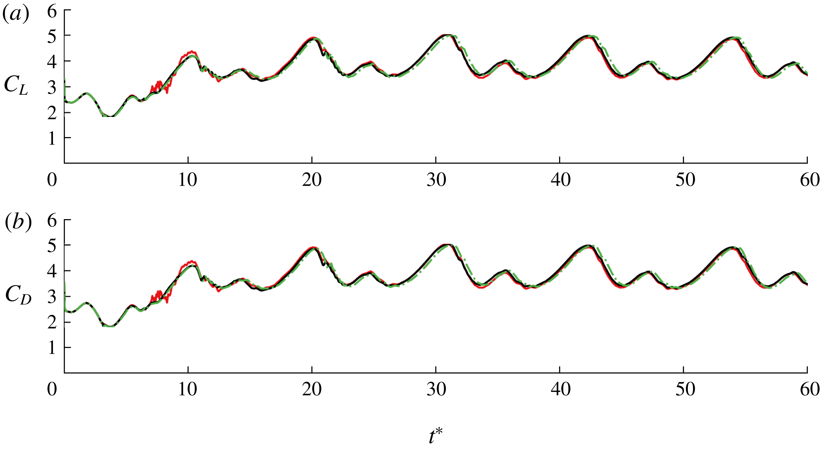
A concern with using a minimum vortex release interval is that it will introduce a $1/T_{min}^{\ast }$ frequency component to the system and cause vortex shedding to lock on to that frequency. We can see that this is not the case in figure 9, as $T_{min}^{\ast }=0.1,~0.2,~0.25$ all predict essentially the same force response. The reduced frequency of this vortex shedding is approximately $fc\sin \unicode[STIX]{x1D6FC}/U=0.067$ , which is lower than the observed frequency in a viscous fluid at this angle, approximately $0.148$ (Fage & Johansen Reference Fage and Johansen1927).

Figure 7.

Comparison of the vorticity distribution in a hybrid model of flow around an impulsively translated plate with $\unicode[STIX]{x1D6FC}=45^{\circ }$ at $t^{\ast }=10$ , using three different choices for minimum time between initiation of new active vortex elements, $T_{min}^{\ast }$ .

Figure 8.

Comparison of the number of vortex elements used over time to simulate impulsive translation at $45^{\circ }$ , using different values of minimum vortex release time interval: $T_{min}^{\ast }=0.1$ (——, red), $T_{min}^{\ast }=0.2$ (——, black) and $T_{min}^{\ast }=0.25$ (– ⋅ – ⋅, green).

Figure 9.

Lift (a) and drag (b) coefficients for impulsive translation at $\unicode[STIX]{x1D6FC}=45^{\circ }$ predicted by the hybrid model with $T_{min}^{\ast }=0.1$ (——, red), $T_{min}^{\ast }=0.2$ (——, black) and $T_{min}^{\ast }=0.25$ (– – –, green).

3.1.2 Translation at $60^{\circ }$ angle of attack

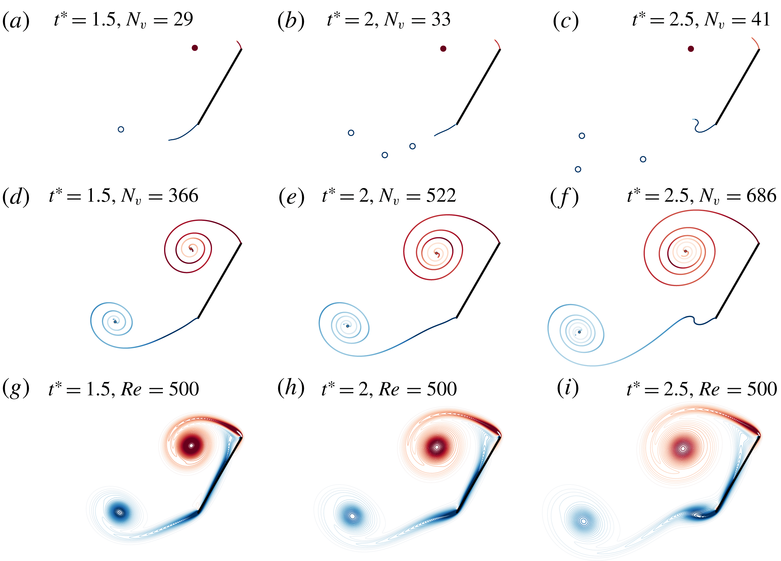
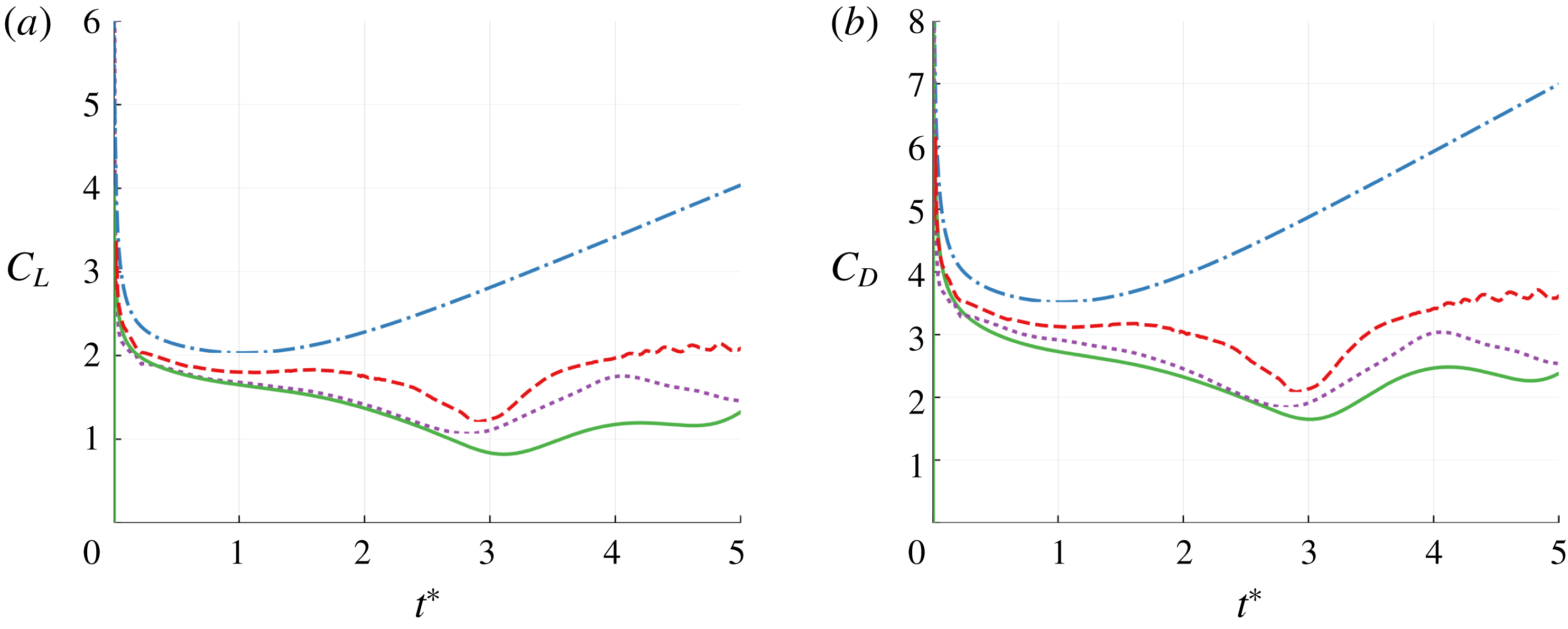
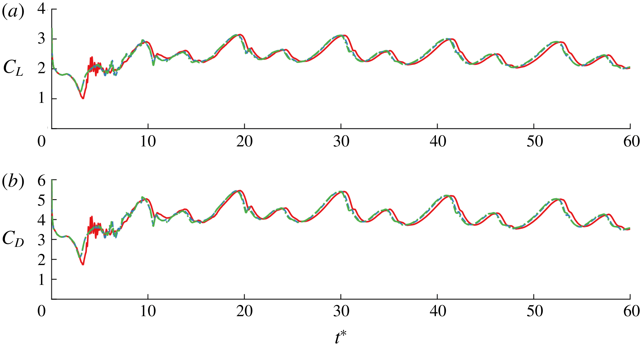
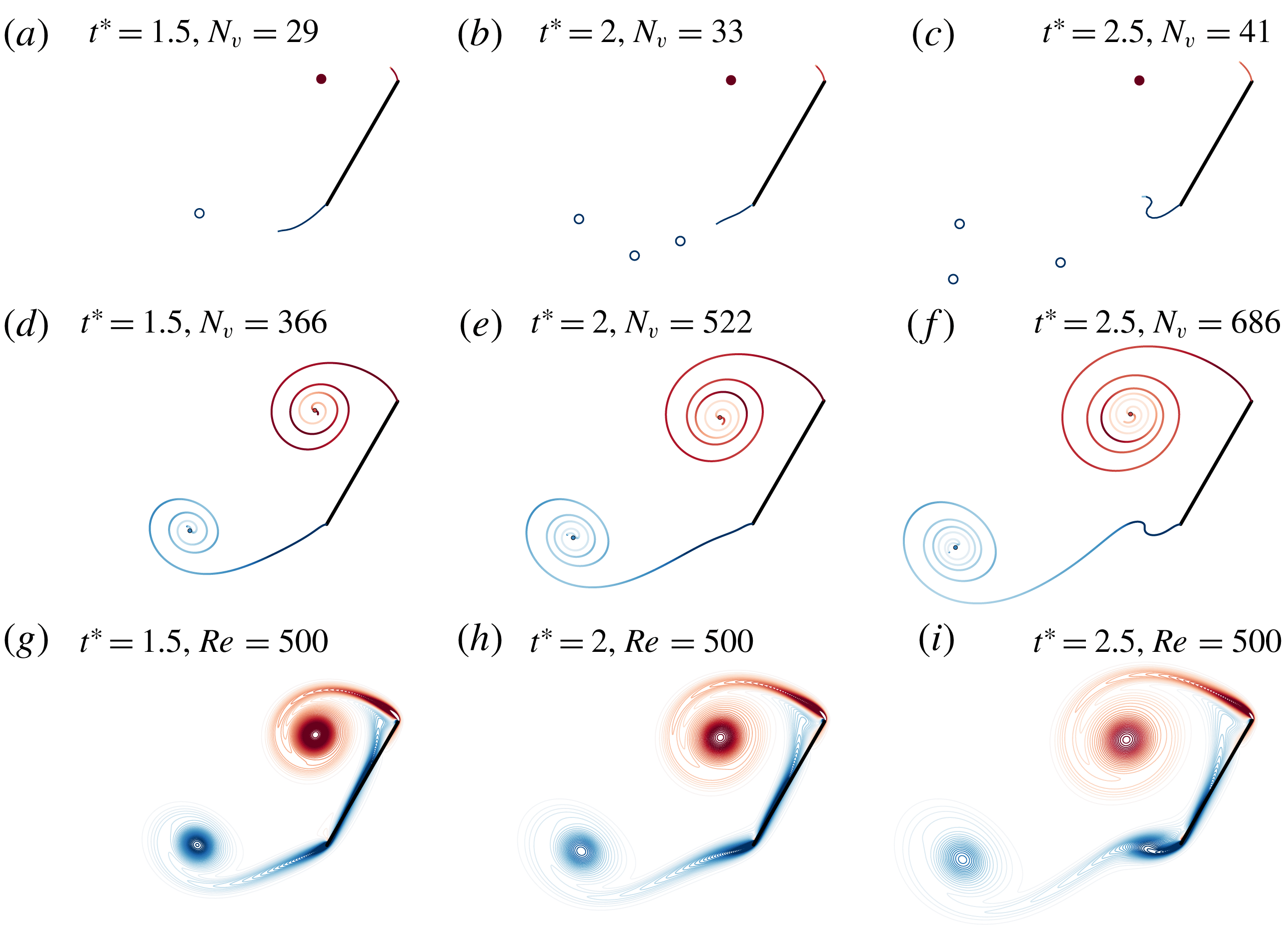
The results for the $\unicode[STIX]{x1D6FC}=60^{\circ }$ case are mostly similar to the $\unicode[STIX]{x1D6FC}=45^{\circ }$ case, but are presented to demonstrate that the choices made and results obtained at the lower angle are not unique. We also use this case to more deeply explore the choices of $B_{F}$ and $T_{min}^{\ast }$ . Figure 10 shows the early-time vorticity distribution predicted by the model, and figures 11 and 12 show the predicted force response. We see that the initial development of the leading- and trailing-edge vortices predicted by the hybrid model is very similar to the high-fidelity simulation results. The hybrid model’s prediction required 0.38 s of CPU time to reach $t^{\ast }=2.5$ and 1.0 s to reach $t^{\ast }=5$ , compared with 0.83 s and 4.6 s, respectively, for the full vortex sheet model. 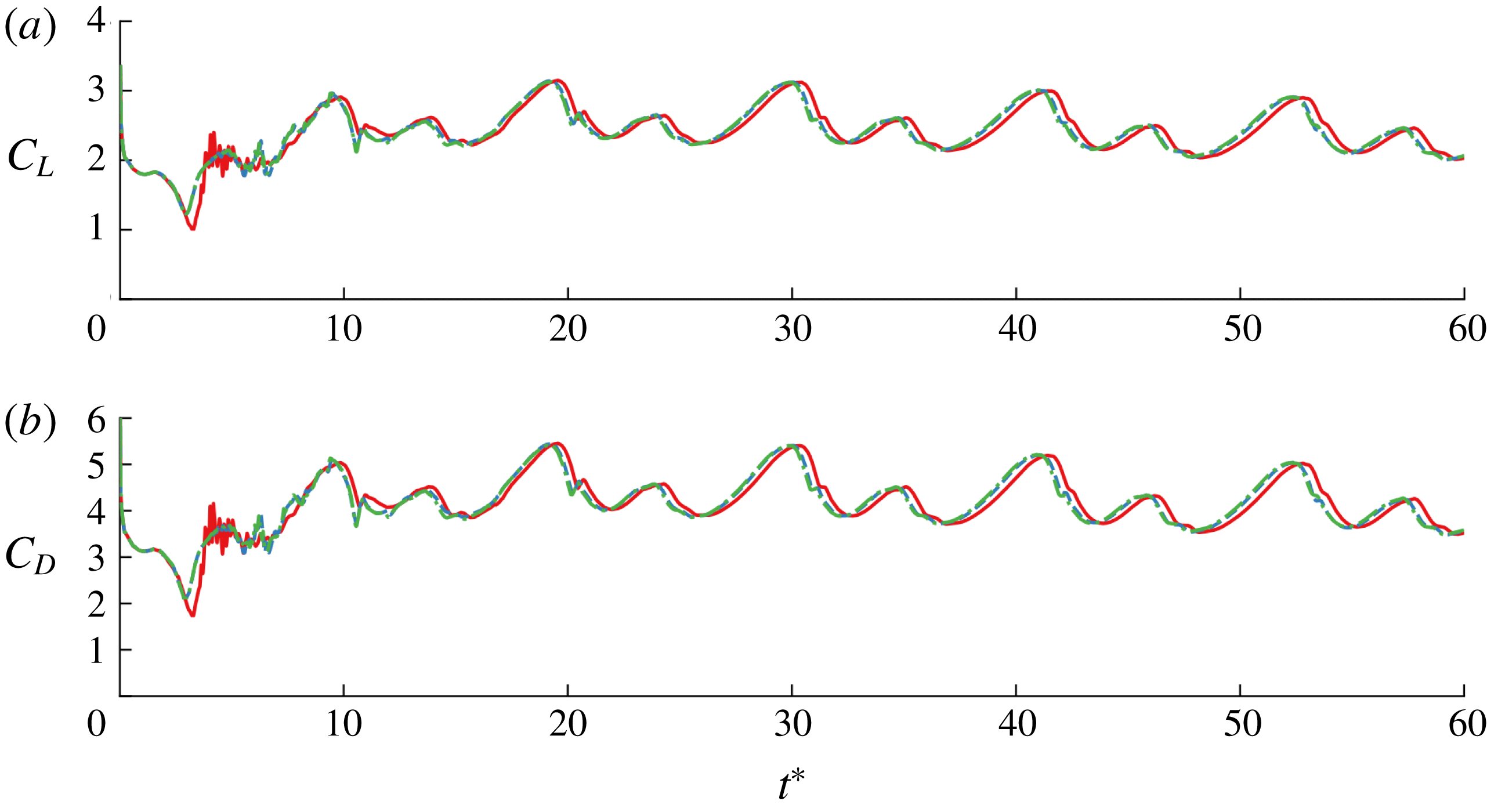As in the $45^{\circ }$ case, the ability to model large-scale vortex shedding allows the model to give a more accurate force response than the Wang & Eldredge model. The shedding frequency in figure 12 is 0.079, still lower than the value at finite Reynolds number. The entire simulation to $t^{\ast }=60$ required 9.4 s of CPU time with the hybrid model using $T_{min}^{\ast }=0.2$ .

Figure 10.

Comparison of the vorticity distribution predicted for a flat plate moved impulsively at $60^{\circ }$ at three different instants between the new hybrid model with $T_{min}^{\ast }=0.2$ (a–c), a full vortex sheet model (d–f) and high-fidelity simulation at $Re=500$ (g–i). 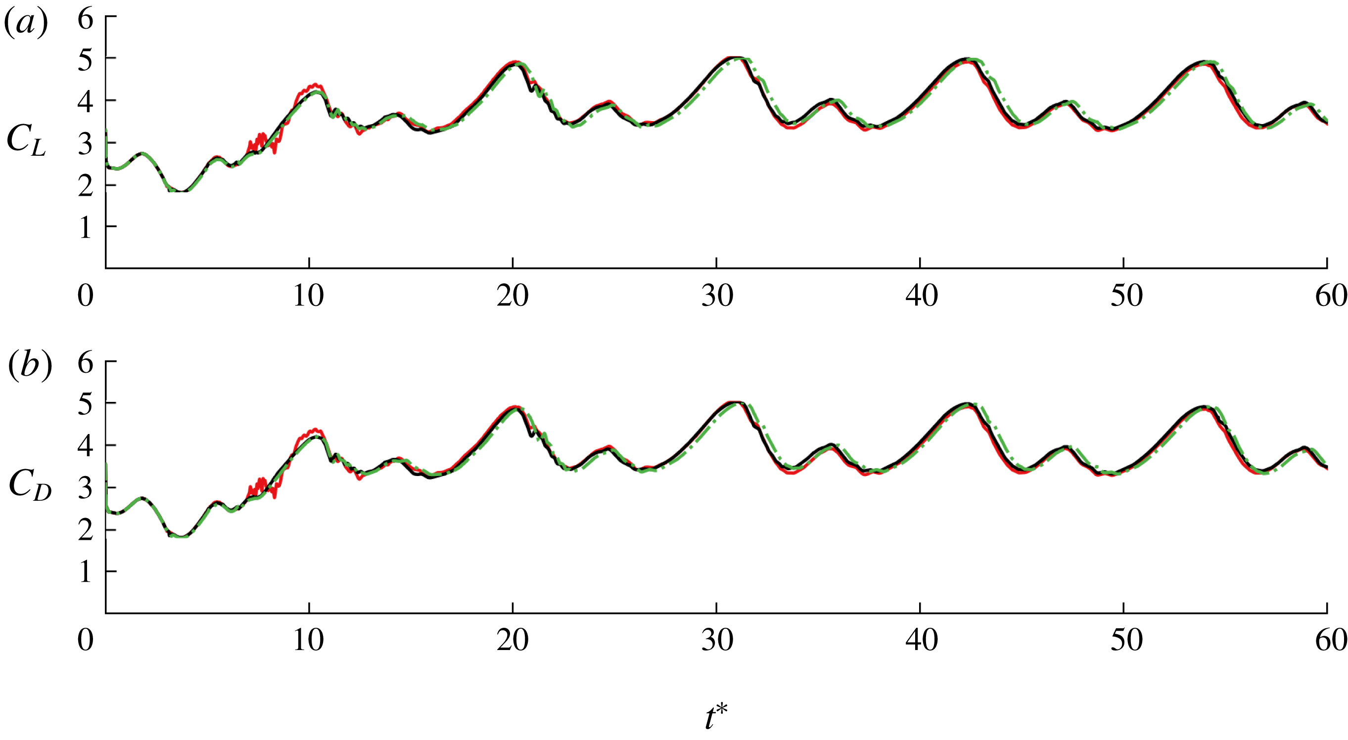The positions of the positive- and negative-strength point vortices are shown with filled and unfilled circles, respectively, and $N$ denotes the total number of vortex elements (including those in the vortex sheets).

Figure 11.

Early-time lift (a) and drag (b) coefficients for impulsive translation at $\unicode[STIX]{x1D6FC}=60^{\circ }$ predicted by the hybrid model with $T_{min}^{\ast }=0.2$ (– –), the vortex sheet model (- - - -), the Wang & Eldredge model (– ⋅ – ⋅) and the high-fidelity simulation at $Re=500$ (——).

Figure 12.

Lift (a) and drag (b) coefficients for impulsive translation at $\unicode[STIX]{x1D6FC}=60^{\circ }$ predicted by the hybrid model with $T_{min}^{\ast }=0.1$ (——, red), $T_{min}^{\ast }=0.2$ (– ⋅ – ⋅, green) and $T_{min}^{\ast }=0.25$ (– –, blue).

Figure 13.

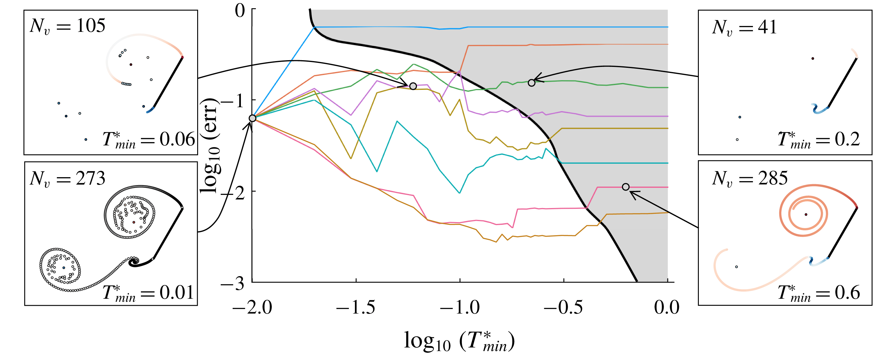
Error versus minimum time between releases of new active point vortices, $T_{min}^{\ast }$ , and tolerance for force discrepancy, $B_{F}$ , for impulsive translation of a flat plate at $60^{\circ }$ angle of incidence, after four convective time units. Error is defined as the r.m.s. difference in force from a reference case, normalized by the $L_{2}$ norm of the reference case force. The reference case is a full vortex sheet, generated with $T_{min}^{\ast }=\infty$ and $B_{F}=0$ . 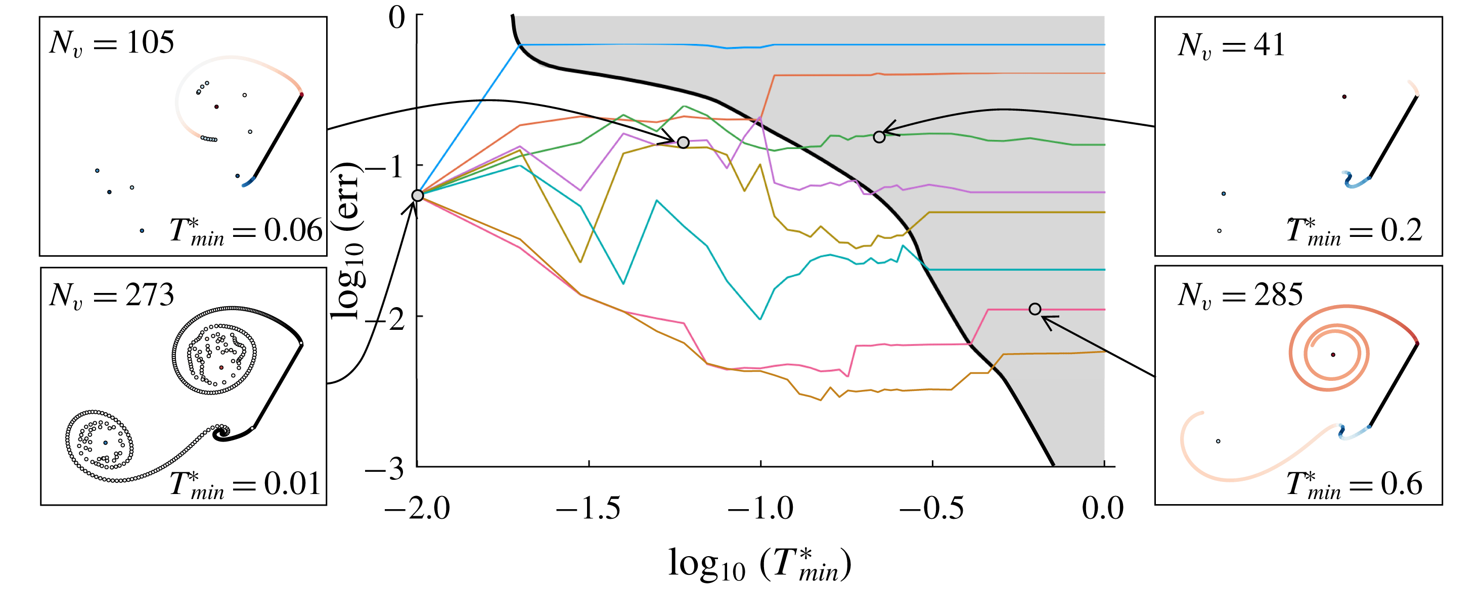The cases shown are: $B_{F}=3\times 10^{-1}$ (blue), $2\times 10^{-1}$ (orange), $10^{-1}$ (green), $6.25\times 10^{-2}$ (purple), $5\times 10^{-2}$ (mustard), $3.5\times 10^{-2}$ (turquoise), $1.25\times 10^{-2}$ (pink) and $6.25\times 10^{-3}$ (brown). The shaded region corresponds to cases with minimal generation of discrete vortex elements. Snapshots of a few sample cases at $t^{\ast }=2.5$ , along with the corresponding number of total vortex elements, are shown.

Figure 14.

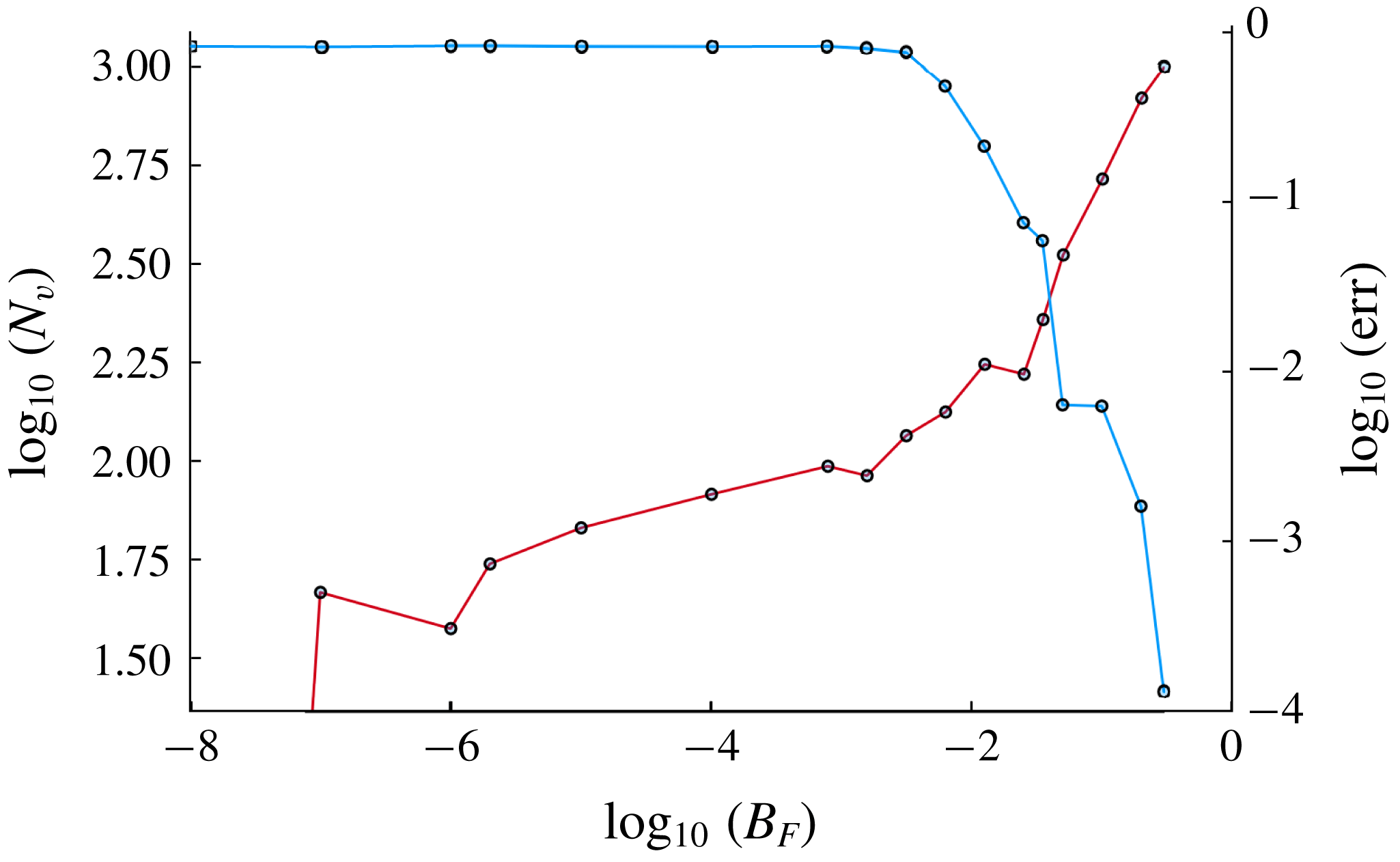
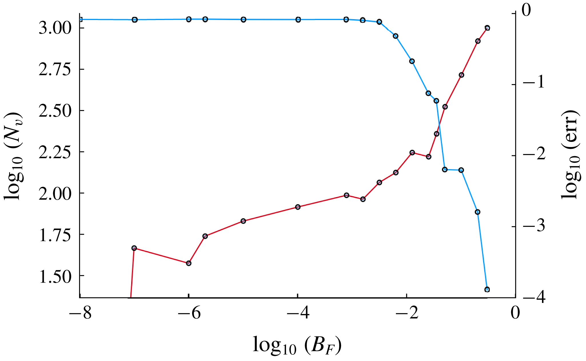
Error (red-brown) and total number of vortex elements (blue) versus tolerance for force discrepancy, $B_{F}$ , with minimum release time, $T_{min}^{\ast }$ , set to $1$ , for impulsive translation of a flat plate at $60^{\circ }$ angle of incidence, after four convective time units. Error is defined as in figure 13.

We use this case to explore the detailed dependences of the results on the tunable parameters $T_{min}^{\ast }$ and $B_{F}$ ; it can be shown that other cases behave similarly. In order to quantitatively assess these dependences, we use the full vortex sheet case (in which $T_{min}^{\ast }=\infty$ and $B_{F}=0$ ) as a reference – the best that can be achieved by an inviscid vortex model – to which all other cases are compared. We use the root-mean-square (r.m.s.) difference of the aerodynamic force from that of the reference, averaged over four convective time units, as a metric for assessment. Figure 13 depicts this error for a large number of choices of $T_{min}^{\ast }$ and $B_{F}$ , plotted on a log–log scale for easier differentiation between the cases. The lower limit of $T_{min}^{\ast }$ corresponds to allowing the release of a new active element at every time step. As expected, a basic discrete vortex element model is achieved in this case, independent of the choice of $B_{F}$ . Several other observations can be made from this plot.

First, for all choices of $B_{F}$ , the error saturates when $T_{min}^{\ast }$ is large. This regime corresponds to a condition in which a minimal number of active vortex elements are released.

The second observation is that the error level at which each choice of $B_{F}$ saturates decays nearly monotonically with $B_{F}$ . This is not surprising, because our definition of error is closely related to the definition of $B_{F}$ : a tolerance for discrepancy in force between siphoning into the active vortex or leaving the circulation in sheet form. This behaviour is more clear in figure 14, in which $T_{min}^{\ast }$ has been set to $1$ and $B_{F}$ is assigned a broad range of values. Eventually, the error falls to exactly zero for a finite choice of $B_{F}$ because there are no segments in the sheet that can be siphoned into the active vortex without exceeding this threshold. In other words, the hybrid model recovers the full vortex sheet result in the simultaneous limits $B_{F}\rightarrow 0$ and $T_{min}^{\ast }\rightarrow \infty$ ; in practice, the result is recovered at finite values of both parameters.

The error results outside of the grey region in figure 13 are more complicated. The force is more sensitive to the parameters when there is a mixture of discrete (inactive) vortex elements and a vortex sheet. However, the error is generally small – less than 10 % for $B_{F}\lesssim 0.1$ . The snapshots of vortex elements reveal examples of the behaviour in different regimes of the parameters.

In summary, it seems desirable for the model to achieve the easily predictable behaviour in the shaded region of figure 13. This requires that we choose $T_{min}^{\ast }$ to be sufficiently large, but not so large that it suppresses the release of new active elements when required by newly formed vortex structures. It is clear that the lower threshold of $T_{min}^{\ast }$ to achieve this predictable regime depends on the choice of $B_{F}$ – smaller $B_{F}$ requires larger $T_{min}^{\ast }$ . Furthermore, we generally should choose $B_{F}$ to balance computational efficiency with error. The plots of the number of vortex elements and the error depicted in figure 14 for each choice of $B_{F}$ provide a useful illustration of this balance. Since relatively large choices of $B_{F}$ (approximately 0.05–0.1) are a safe choice, and we seek smaller $T_{min}^{\ast }$ so that active elements are available when needed to efficiently capture the formation of structures, it is generally sufficient to choose $T_{min}^{\ast }\approx 0.1$ – $0.3$ .

Figure 15.

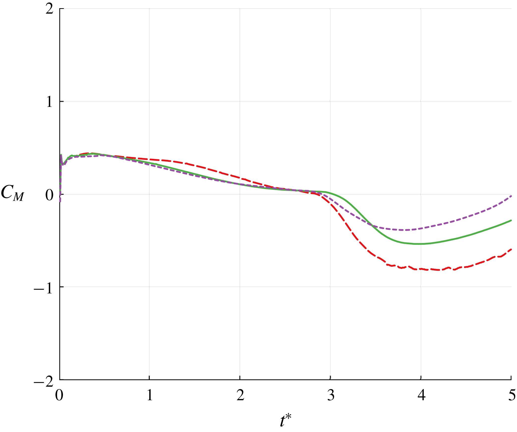
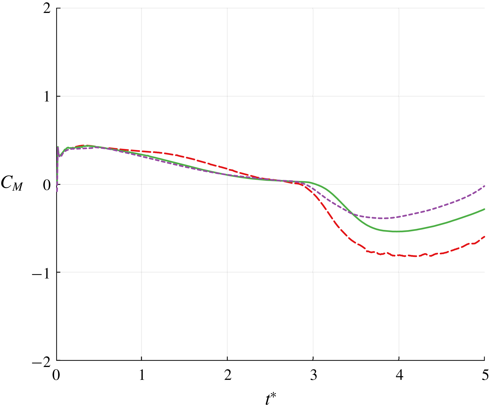
Early-time moment coefficient (about the centroid) for impulsive translation at $\unicode[STIX]{x1D6FC}=60^{\circ }$ predicted by the hybrid model with $T_{min}^{\ast }=0.2$ and $B_{F}=10^{-1}$ (– –, red), $T_{min}^{\ast }=0.2$ and $B_{F}=5\times 10^{-2}$ (——, green), and the vortex sheet model (- - - -, purple).

Thus far, we have used only force to measure the quality of the class of hybrid inviscid vortex models proposed in this work. However, because the method design is based explicitly on force – both in the velocity correction procedure described in § 2 and in the tunable parameter, $B_{F}$ – one might wonder about the behaviour of pitching moment. In figure 15, for this case of impulsive translation at $60^{\circ }$ , we plot the moment coefficient, $C_{M}$ , evaluated about the plate centroid, predicted by two versions of the hybrid method with different values of $B_{F}$ as well as by the full vortex sheet model. For the first several convective times, all of the methods agree well; they tend to deviate at later times, more so than they did in force. This additional sensitivity is expected, since the moment weights the relative locations of vortex elements more heavily than force. However, it is important to observe that the moment is smooth in all cases, exhibiting no spurious jumps while circulation is transferred from the sheet into active point vortices or when new active vortices are released. Furthermore, the moment tends to converge towards the sheet model as $B_{F}$ decreases.

3.2 Pitch-up while translating

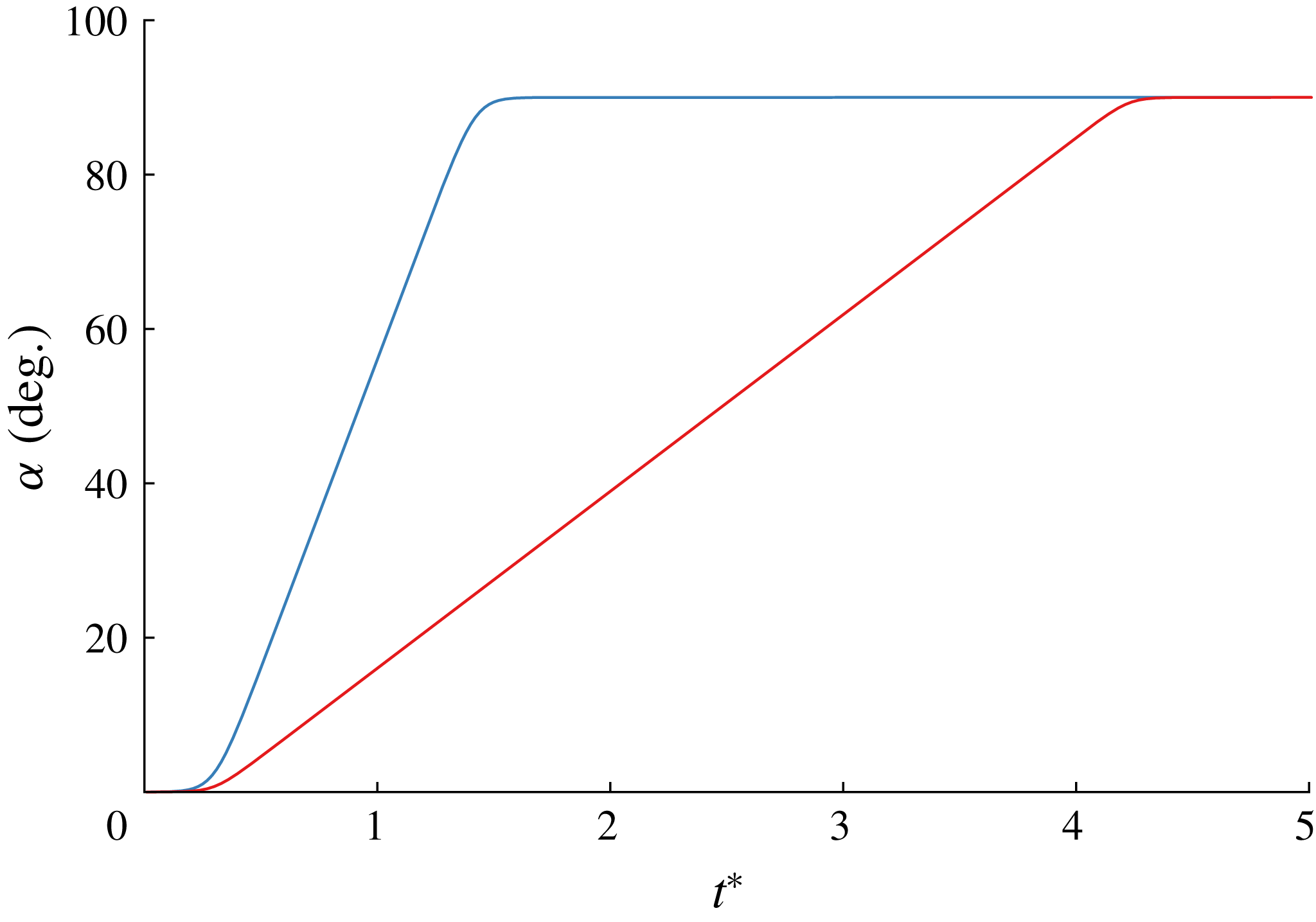
In this section we consider the flat plate translating at constant velocity $U$ and simultaneously pitching about its leading edge from angle of attack $0$ to $\unicode[STIX]{x1D6FC}_{f}=\unicode[STIX]{x03C0}/2$ over an interval that starts at $t_{1}$ and ends at $t_{2}$ , for a nominal pitch rate of $\dot{\unicode[STIX]{x1D6FC}}_{0}:=\unicode[STIX]{x1D6FC}_{f}/(t_{2}-t_{1})$ . The pitch-up manoeuvre follows a smoothed linear ramp given by

(3.1)

$$\begin{eqnarray}\displaystyle \unicode[STIX]{x1D6FC}(t)=\frac{K}{a}G(t), & & \displaystyle\end{eqnarray}$$

where $K:=\dot{\unicode[STIX]{x1D6FC}}_{0}c/(2U)$ is the non-dimensional pitch rate,

(3.2)

$$\begin{eqnarray}\displaystyle G(t)=\log \left[\frac{\cosh (aU(t-t_{1})/c)}{\cosh (aU(t-t_{2})/c)}\right]+aU(t_{2}-t_{1})/c & & \displaystyle\end{eqnarray}$$

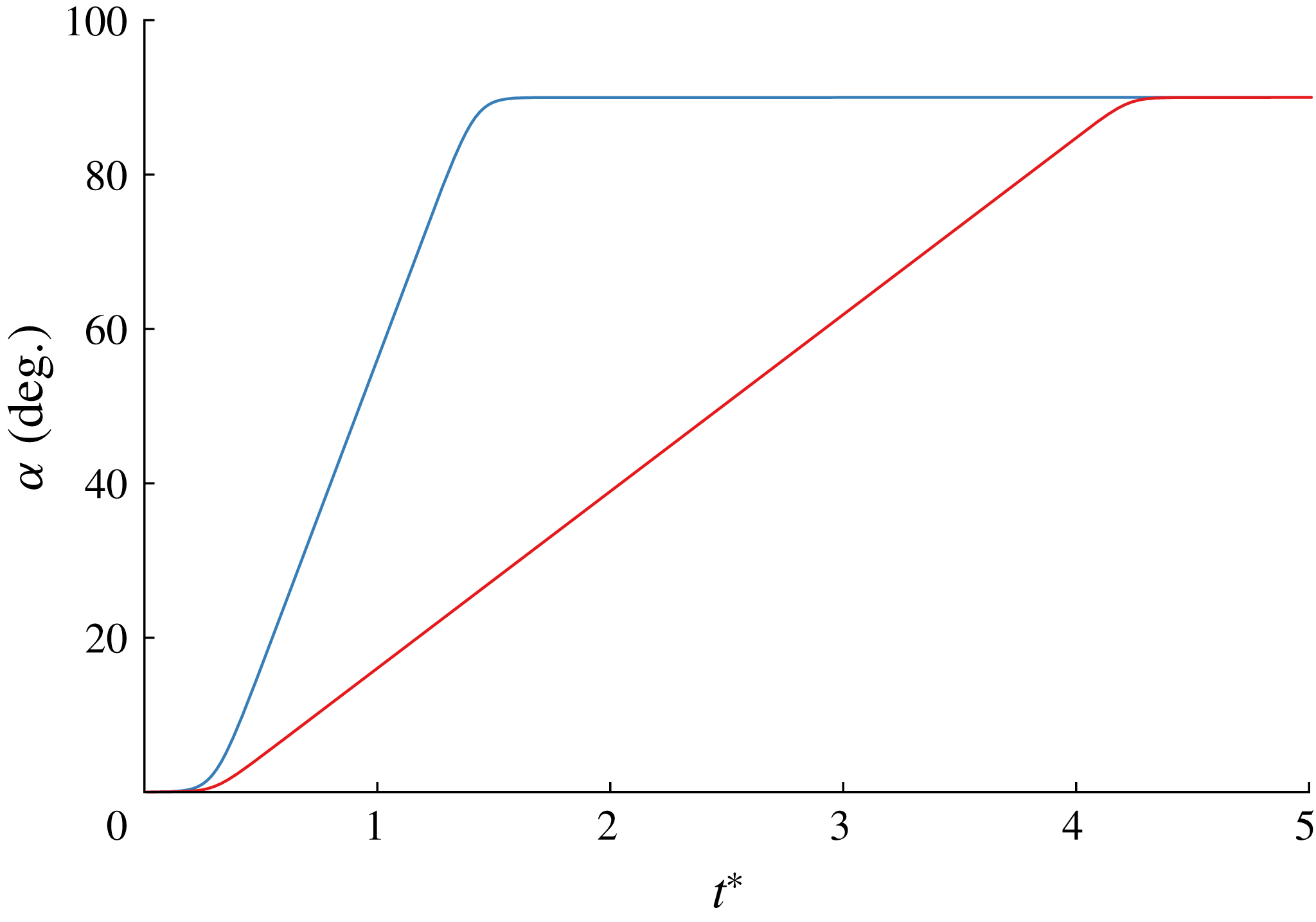
is a smooth ramp function and $a$ is a smoothing parameter that we set to 11 (Eldredge, Wang & Ol Reference Eldredge, Wang and Ol2009). The time histories of the angle of attack for both values of $K$ used in this study are shown in figure 16. The initial instant of the pitch manoeuvre, $Ut_{1}/c$ , is set to $0.3$ ; the completion of the manoeuvre, $Ut_{2}/c$ , is determined by this initial instant and by $K$ .

Figure 16.

Histories of angle of attack of flat plate for pitch-up problem: $K=0.7$ (blue) and $K=0.2$ (red).

Figure 17.

Comparison of the vorticity distribution predicted for a flat plate pitching with $K=0.7$ at two different instants between the hybrid model with $T_{min}^{\ast }=0.1$ (a,b) and a high-fidelity simulation at $Re=1000$ (c,d) at $\unicode[STIX]{x1D6FC}=33^{\circ }$ (a,c) and $\unicode[STIX]{x1D6FC}=90^{\circ }$ (b,d).

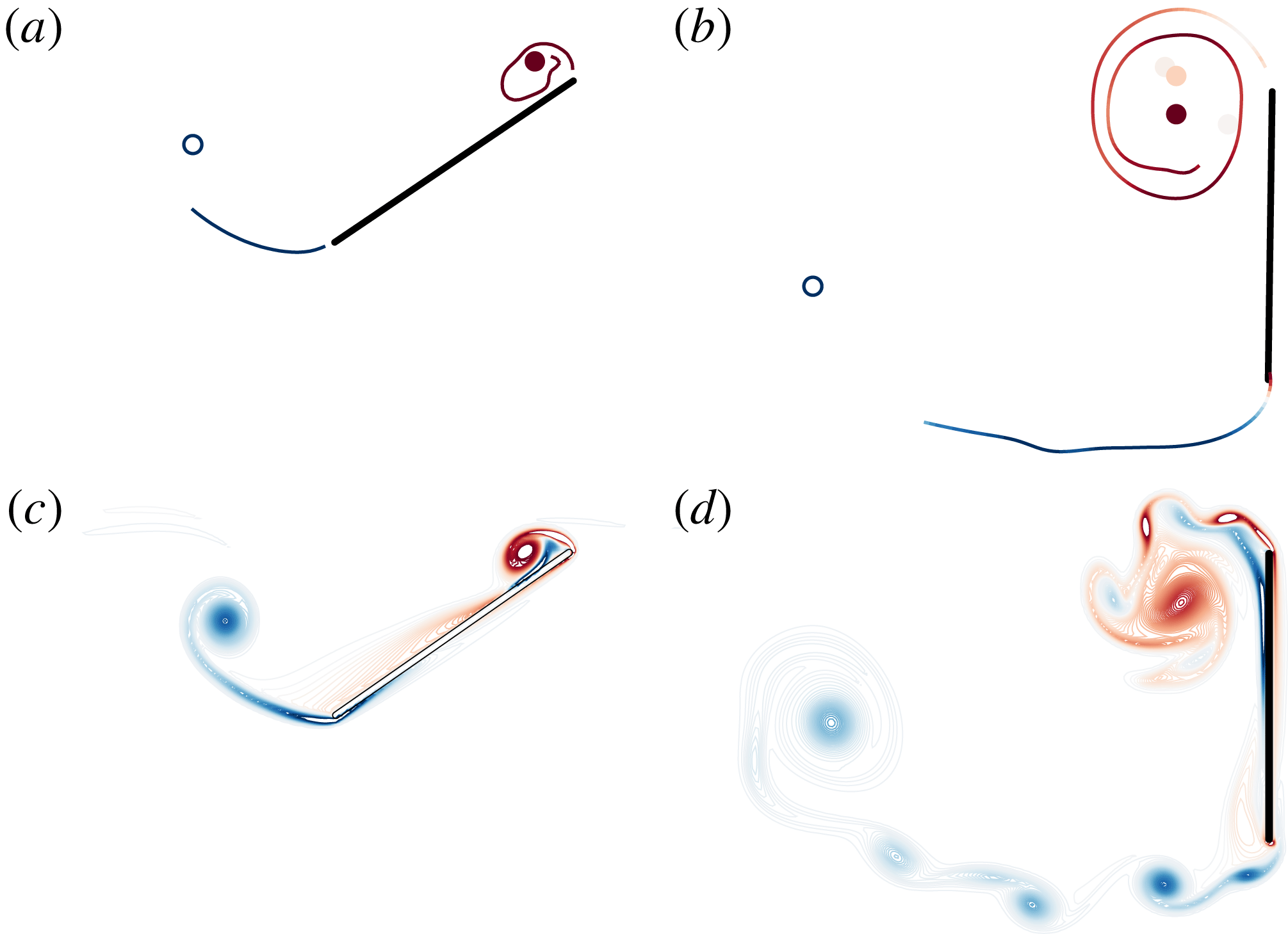
We first consider a pitch-up manoeuvre with $K=0.7$ (see figure 17). Unlike the cases with high angle of attack described previously, the extended amount of time that the plate spends at low angles of attack makes it challenging to release vortex sheets from the leading edge. If we apply the Kutta condition, then it requires the vortex sheet to leave the plate tangent to the plate, in a direction nearly opposite the relative free stream. Furthermore, this leading-edge sheet interacts strongly (and non-physically) with the plate due to its close proximity at low angle of attack. These challenges are somewhat alleviated if we use the leading-edge suction criterion proposed by Ramesh et al. (Reference Ramesh, Gopalarathnam, Granlund, Ol and Edwards2014), where new vortex elements are only endowed with non-zero strength if the leading-edge suction parameter (LESP) exceeds a critical threshold (see (A 8) in § A.1). For all of our pitch-up cases, we will use a critical LESP value of $\text{LESP}_{c}=0.1$ , similar to that reported by Ramesh et al. (Reference Ramesh, Gopalarathnam, Granlund, Ol and Edwards2014). However, it must be noted that, by relaxing the Kutta condition, the singular velocity at the leading edge will tend to introduce numerical instability into the vortex sheet. Additionally, at very low angles of attack, the circulation released at the leading edge is so weak that new vortex elements tend to remain near the plate’s surface instead of rolling into a sheet. The sustained proximity of these point vortices to the plate introduces large fluctuations in the force response due to the large tangential motions generated by the no-flow-through condition.

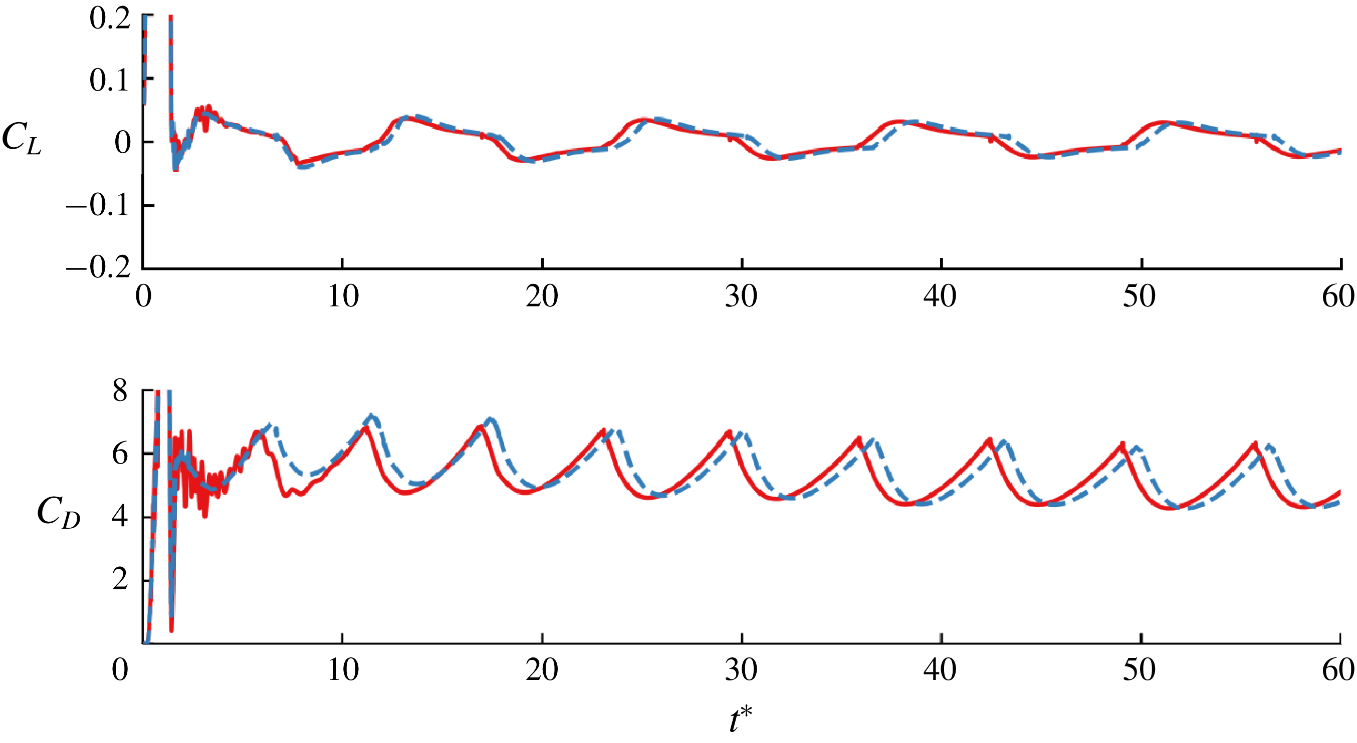
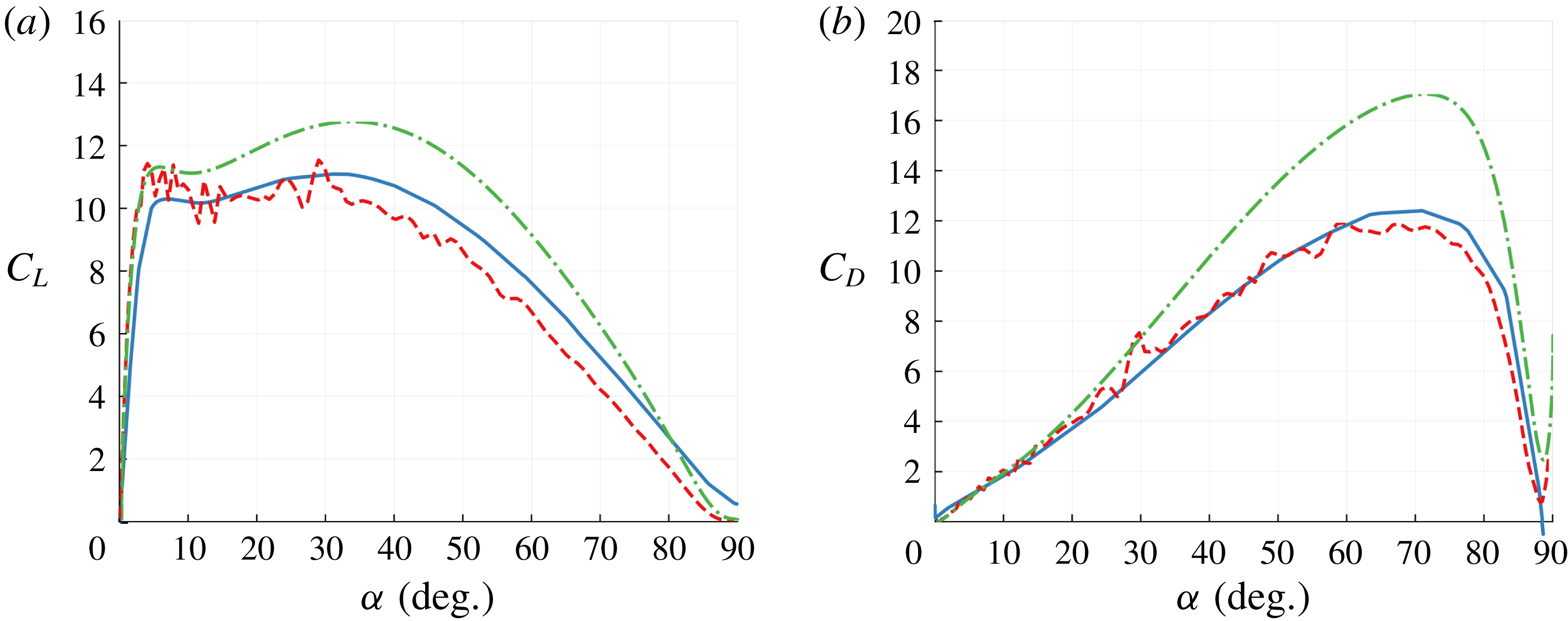
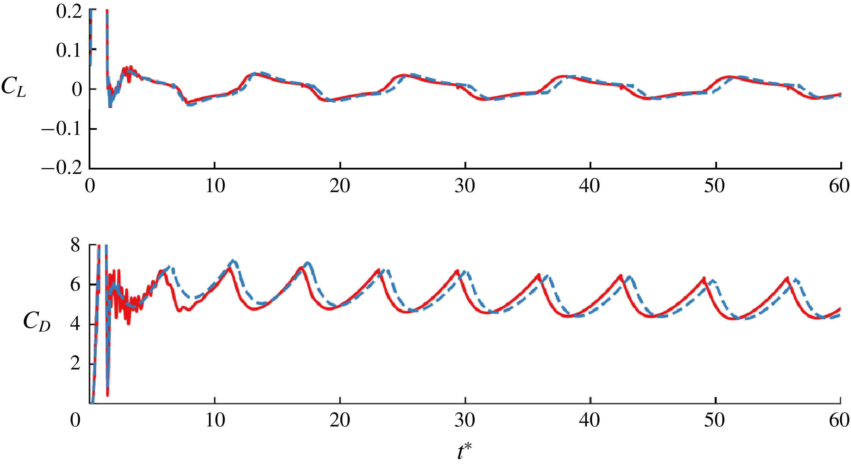
Transferring circulation from the sheet to the active point vortex not only suppresses the emergence of numerical instabilities in the sheet, but also tends to move vortex elements away from the plate surface, thus reducing the noise in the force response. Figure 18 shows a comparison of the lift and drag coefficients during the pitch-up motion. In vortex models with only variable-strength point vortices, such as the Wang & Eldredge (Reference Wang and Eldredge2013) model, the vorticity flux from the leading edge goes directly into the active leading-edge vortex. The fast growth of such a point vortex means that these models tend to overpredict the lift on the plate. In the proposed hybrid model, the leading-edge circulation is distributed between the active point vortex and the vortex sheet, giving a more accurate force response. However, some noise remains in the early force response as the leading-edge vortex sheet rolls up and interacts strongly with the bound vortex sheet of the plate. Figure 19 shows the lift and drag coefficients as the flow settles down to periodic bluff-body shedding past a plate at normal incidence. The results are mildly sensitive to the choice of $T_{min}^{\ast }$ , exhibiting a slightly different prediction of the onset of shedding.

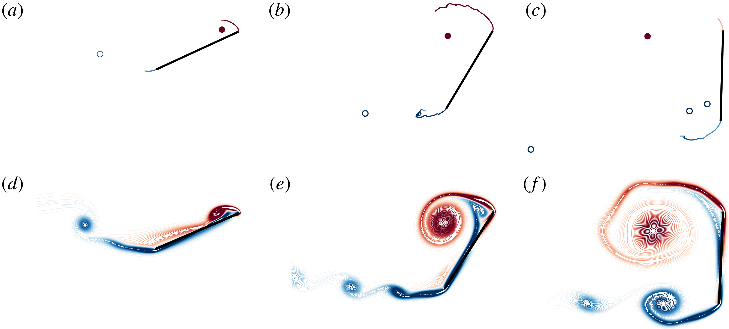
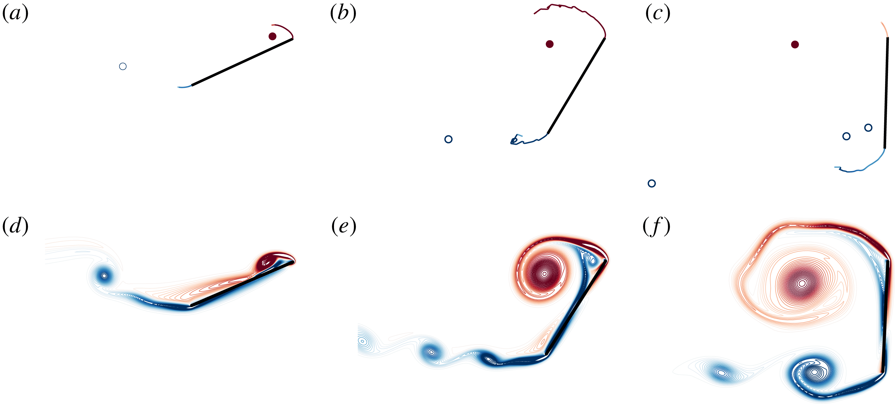
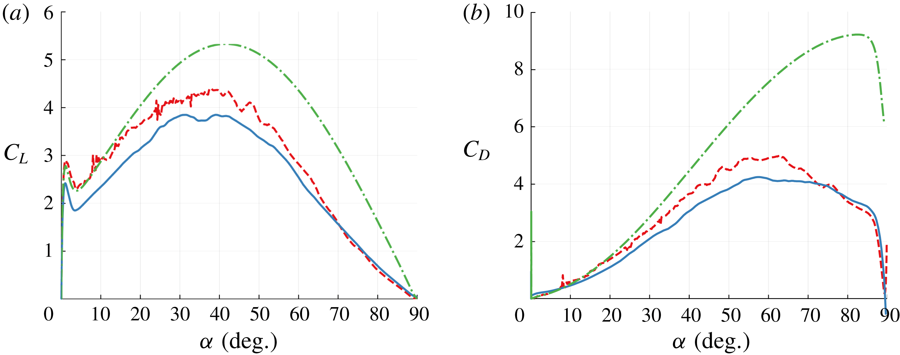
For the $K=0.2$ pitch-up case, the plate spends even longer in a low-angle-of-attack configuration. From both the vorticity distribution in figure 20 and the predicted force response in figure 21, we observe noise of comparable magnitude compared to the $K=0.7$ case. The frequency of this noise is also comparable, but looks larger when force is plotted versus angle of attack since the traversal of this range of angles occurs more slowly at $K=0.2$ . In these results, the circulation transfer rate is just high enough to keep the vortex sheets short and stable until the plate reaches a high angle of attack. Again, more accurate (but somewhat noisier) results are achieved than for the variable-strength vortex model of Wang & Eldredge (Reference Wang and Eldredge2013).

Figure 18.

Early-time lift (a) and drag (b) coefficients for a pitch-up manoeuvre at $K=0.7$ predicted by the hybrid model with $T_{min}^{\ast }=0.1$ (– –, red), the Wang & Eldredge model (– ⋅ – ⋅, green) and high-fidelity simulation results at $Re=1000$ (——, blue).

Figure 19.

Comparison of the long-term lift and drag coefficients for a pitch-up manoeuvre at $K=0.7$ predicted with $T_{min}^{\ast }=0.1$ (——, red) and $T_{min}^{\ast }=0.2$ (– –, blue).

Figure 20.

Comparison of the vorticity distribution predicted for a flat plate pitching with $K=0.2$ at two different instants between the hybrid model with $T_{min}^{\ast }=0.2$ (a–c) and a high-fidelity simulation at $Re=1000$ (d–f) at $\unicode[STIX]{x1D6FC}=23^{\circ }$ (a,d), $\unicode[STIX]{x1D6FC}=57^{\circ }$ (b,e) and $\unicode[STIX]{x1D6FC}=87^{\circ }$ (c,f).

Figure 21.

Early-time lift (a) and drag (b) coefficients for a pitch-up manoeuvre at $K=0.2$ predicted by the hybrid model with $T_{min}^{\ast }=0.2$ (– –, red), the Wang & Eldredge model (– ⋅ – ⋅, green) and high-fidelity simulation results at $Re=1000$ (——, blue).

3.3 Oscillatory pitching and heaving

Figure 22.

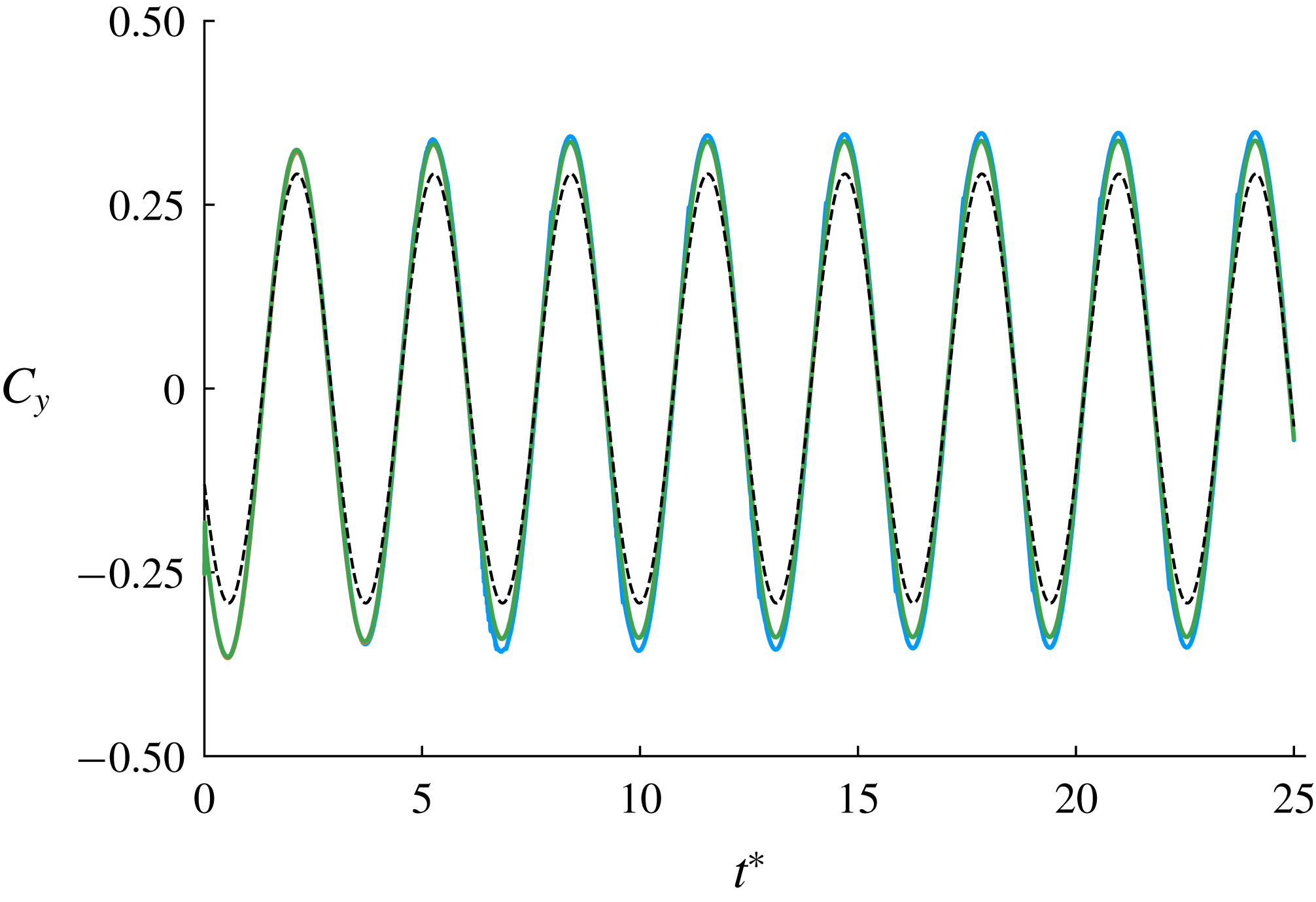
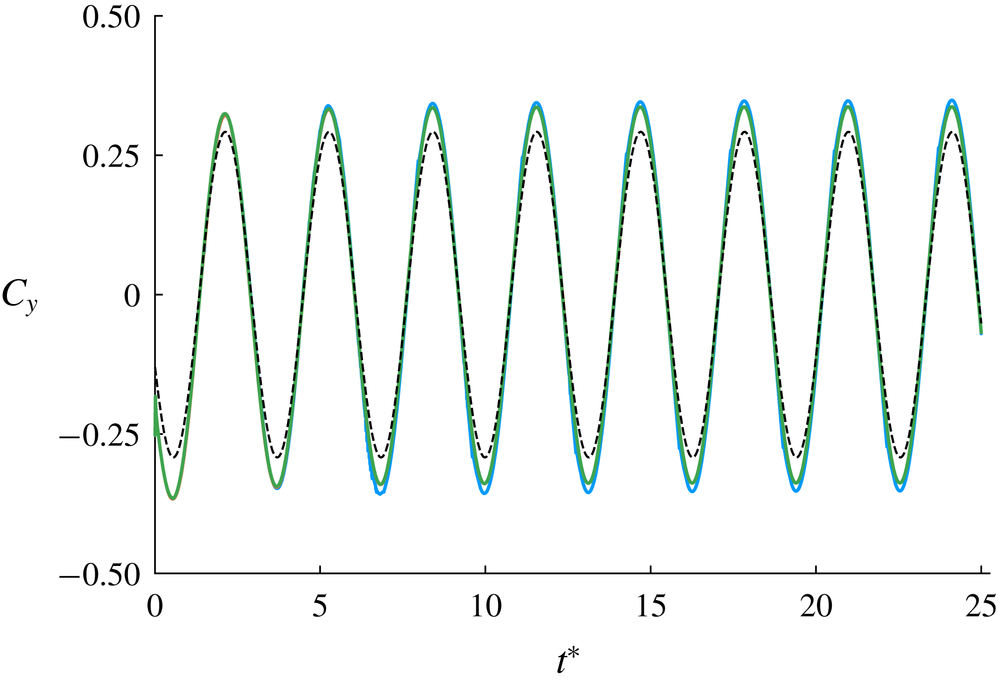
Comparison of the lift coefficient generated by oscillatory pitching and heaving at reduced frequency $\unicode[STIX]{x1D705}=1$ , heave amplitude $h_{0}/c=0.05$ and pitch amplitude $\unicode[STIX]{x1D6FC}_{0}=5^{\circ }$ , predicted with $T_{min}^{\ast }=0.1$ (——, blue), $T_{min}^{\ast }=0.4$ (——, red) and full vortex sheet (——, green). The Theodorsen solution (– –) is shown for reference. Both hybrid method results use $B_{F}=1.75\times 10^{-2}$ .

Figure 23.

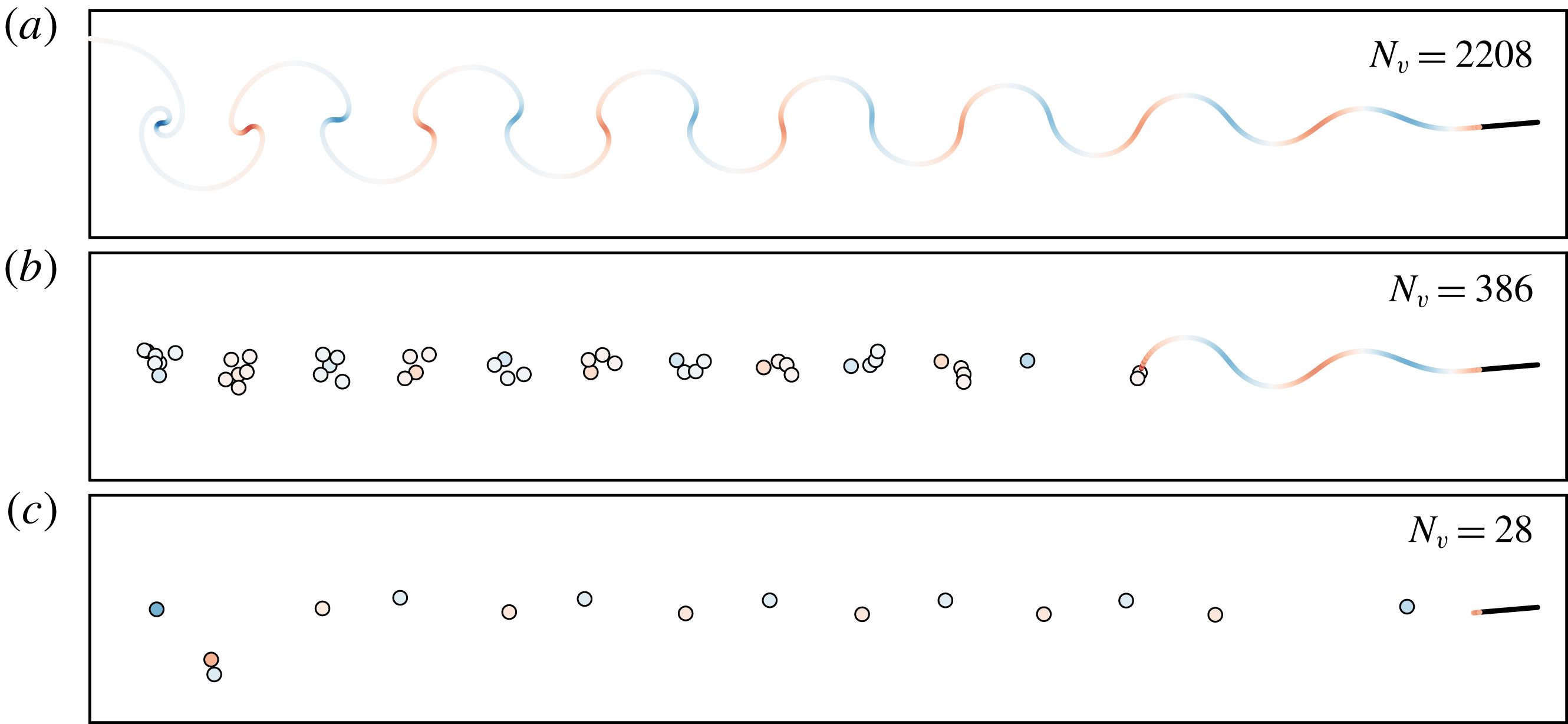
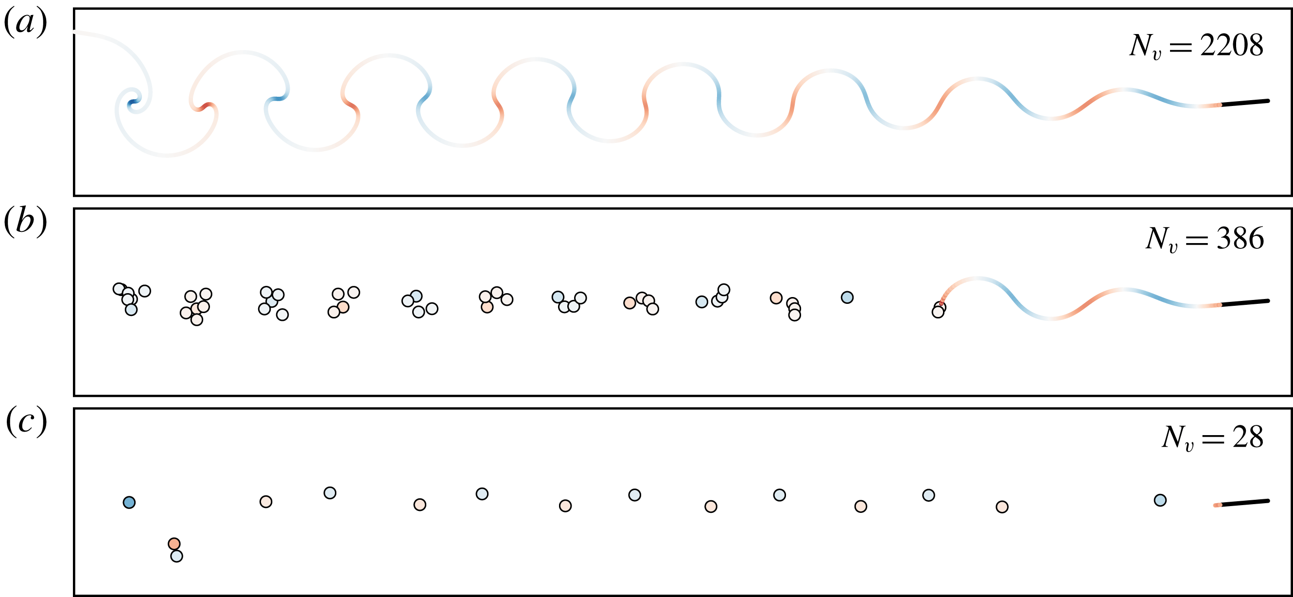
Snapshots of the vorticity distribution at $t^{\ast }=25$ generated by oscillatory pitching and heaving at reduced frequency $\unicode[STIX]{x1D705}=1$ , heave amplitude $h_{0}/c=0.05$ and pitch amplitude $\unicode[STIX]{x1D6FC}_{0}=5^{\circ }$ , predicted with full vortex sheet (a), hybrid model with $T_{min}^{\ast }=0.4$ (b) and hybrid model with $T_{min}^{\ast }=0.1$ (c). Both hybrid method results use $B_{F}=1.75\times 10^{-2}$ .

In this last demonstration case, we consider the common motion of oscillatory pitching and heaving of a flat plate, defined by steady horizontal translation at speed $U$ , with a pitching motion,

(3.3)

$$\begin{eqnarray}\displaystyle \unicode[STIX]{x1D6FC}(t)=\unicode[STIX]{x1D6FC}_{0}\sin (\unicode[STIX]{x1D714}t+\unicode[STIX]{x1D719}), & & \displaystyle\end{eqnarray}$$

about an axis that oscillates vertically, at instantaneous position

(3.4)

$$\begin{eqnarray}\displaystyle h(t)=h_{0}\sin (\unicode[STIX]{x1D714}t). & & \displaystyle\end{eqnarray}$$

The general problem is parametrized by the pitch amplitude $\unicode[STIX]{x1D6FC}_{0}$ , the heave amplitude $h_{0}/c$ , the reduced frequency $\unicode[STIX]{x1D705}:=\unicode[STIX]{x1D714}c/(2U)$ and the pitching phase lead $\unicode[STIX]{x1D719}$ . This phase lead is held constant at $\unicode[STIX]{x03C0}/2$ and the pitch axis is located at the quarter chord.

At small amplitudes $\unicode[STIX]{x1D6FC}_{0}$ and $h_{0}/c$ , the theoretical prediction of Theodorsen (Reference Theodorsen1935) is approximately valid and can be used as a reference. An example of such a case is depicted in figure 22. Here, the amplitudes of pitching and heaving are set to $\unicode[STIX]{x1D6FC}_{0}=5^{\circ }$ and $h_{0}/c=0.05$ , respectively, and the reduced frequency is $\unicode[STIX]{x1D705}=1$ . We have set the critical value of $\text{LESP}$ to a large value ( $10$ ) to prevent the release of any vorticity from the leading edge. The vertical force coefficient generated by this motion only slightly exceeds the prediction from the flat wake model of Theodorsen. Two different versions of the hybrid model are used for comparison, one in which $T_{min}^{\ast }=0.4$ and another in which $T_{min}^{\ast }=0.1$ . The force discrepancy parameter, $B_{F}$ , has been set smaller ( $1.75\times 10^{-2}$ ) than in previous cases due to the relatively smaller strengths in the wake vortex sheet in this weak oscillatory motion. This choice ensures that the other parameter, $T_{min}^{\ast }$ , generates different behaviours when varied; see figure 13 for the rationale for this. The forces predicted by both hybrid models agree well with the full vortex sheet case; the relative errors compared to the vortex sheet case are $0.0042$ for $T_{min}^{\ast }=0.4$ (indistinguishable from the vortex sheet result in figure 22) and $0.050$ for $T_{min}^{\ast }=0.1$ .

As figure 23 shows, this wake does not remain flat, but undergoes the expected instability of a vortex sheet with sinusoidal strength distribution. The two hybrid models exhibit different representations of this instability, and their difference reveals some subtlety in the dependence on $T_{min}^{\ast }$ that was not exhibited in previous cases. For the larger $T_{min}^{\ast }$ , more discrete elements are created and these elements tend to cluster into vortex structures, spaced at an interval equal to the sheet wavelength. In contrast, for the smaller $T_{min}^{\ast }$ , only a single discrete element comprises each vortex structure, and the overall population of elements is very small. At first, this behaviour seems counterintuitive, since previous cases have shown that more discrete elements tend to be generated when the minimum waiting time between the formation of new active elements is reduced. However, it is important to remember that a new active element can only be produced if the current active element can no longer siphon off any of the sheet without exceeding the threshold for error in impulse (step (iv) of the algorithm). When this minimum waiting time is small ( $T_{min}^{\ast }=0.1$ or, in fact, any smaller value still greater than the time step size), then the siphoning is allowed to continue unabated, but stops naturally once per half-cycle when the feeding sheet, with sinusoidally varying strength, reaches an extremum. When $T_{min}^{\ast }$ is larger, this natural process still occurs, but, due to small disruptions in impulse that truncate the siphoning, a train of active elements is created in each half-cycle, which subsequently aggregate into a cluster.

For more general amplitudes of motion, the problem has been studied extensively both experimentally and computationally (Anderson et al. Reference Anderson, Streitlien, Barrett and Triantafyllou1998; Kinsey & Dumas Reference Kinsey and Dumas2008). The character of the flow generated by the plate motion depends on the so-called ‘feathering parameter’ (Anderson et al. Reference Anderson, Streitlien, Barrett and Triantafyllou1998),

(3.5)

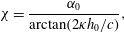$$\begin{eqnarray}\displaystyle \unicode[STIX]{x1D712}=\frac{\unicode[STIX]{x1D6FC}_{0}}{\arctan (2\unicode[STIX]{x1D705}h_{0}/c)}, & & \displaystyle\end{eqnarray}$$

which approximately controls the maximum effective angle of attack. A feathering parameter close to unity restricts this maximum angle to small values, and in such circumstances the flow is expected to remain attached over the plate. In contrast, larger or smaller values of this parameter will induce separation at the leading edge. For feathering parameters larger than unity, the plate is expected to extract energy from the incident flow, whereas the plate generates a propulsive force for smaller values (Anderson et al. Reference Anderson, Streitlien, Barrett and Triantafyllou1998; Kinsey & Dumas Reference Kinsey and Dumas2008).

In the previous case of pitch-up, we discussed the challenges inherent to inviscid models of releasing vorticity from the leading edge at moderate angles of attack. These challenges are more formidable in an oscillatory problem, as the plate will interact strongly with any leading-edge vorticity that lingers in its vicinity for more than one oscillation cycle. The proposed hybrid method does not overcome these challenges. Thus, for the purposes of demonstrating this method on a plate in oscillatory motion, we focus on two cases in which the maximum angle of attack ( $20^{\circ }$ ), though still likely to lead to leading-edge flow separation, is modest enough that suppressing the release of vorticity from this edge still leads to a reasonable prediction of the true behaviour. In both cases, we compare the hybrid model’s prediction with that of a model in which a full vortex sheet is released from the trailing edge.

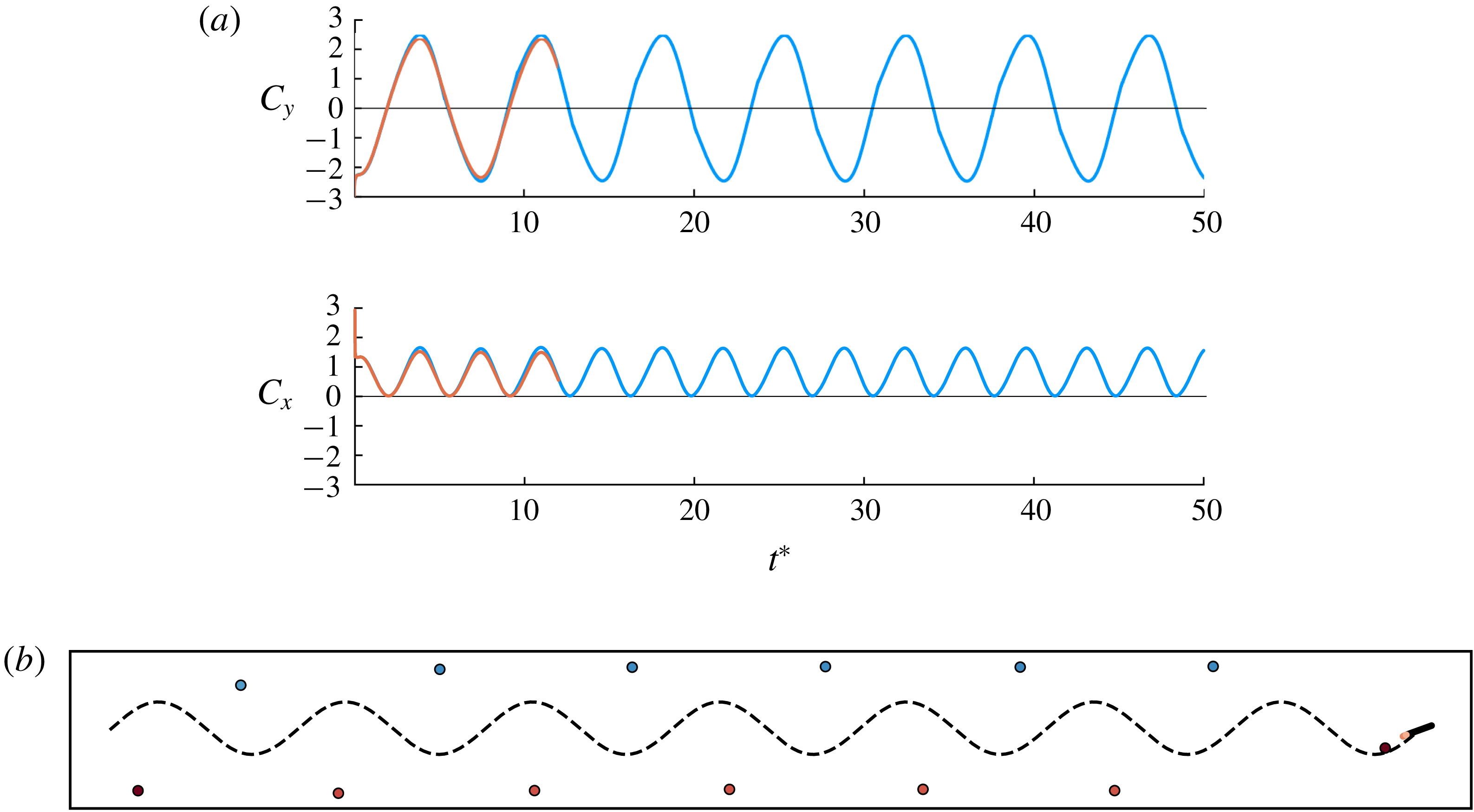
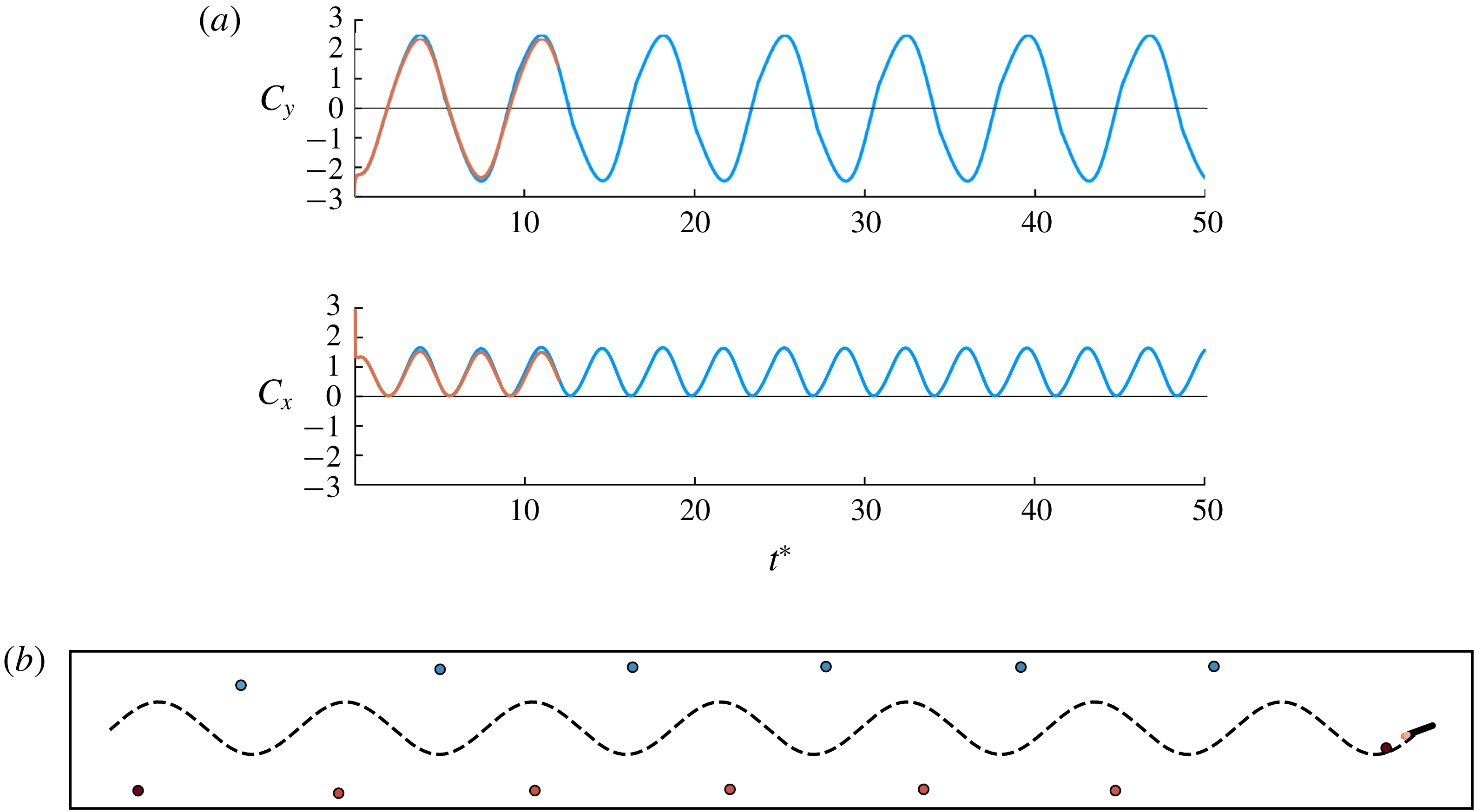
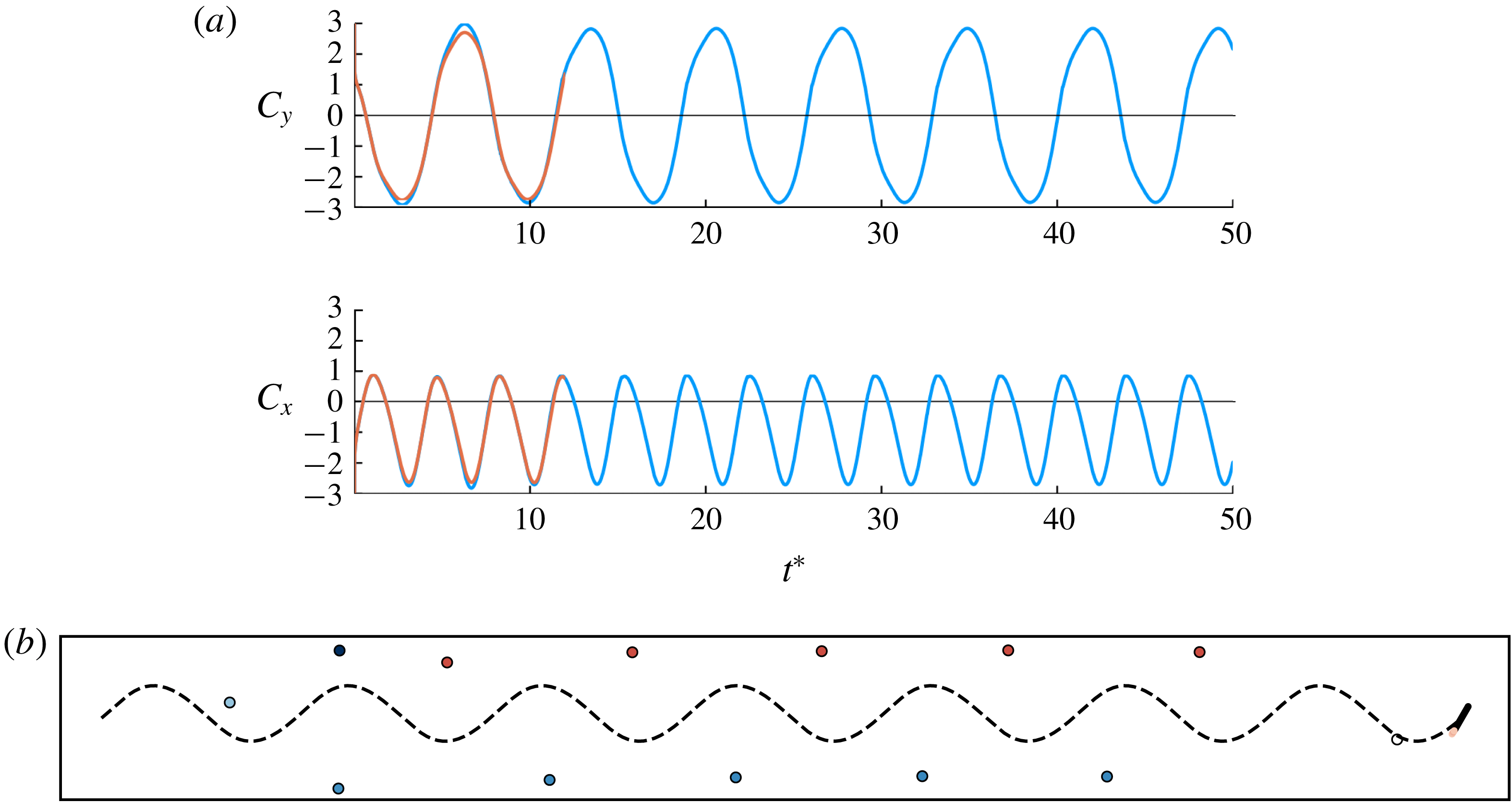
The heave amplitude for both cases is $h_{0}/c=1$ and the reduced frequency is $\unicode[STIX]{x1D705}=0.44$ . Figure 24 depicts the results for a case in which the pitch amplitude is $60^{\circ }$ , leading to a feathering parameter equal to $1.45$ . As expected from the results of Anderson et al. (Reference Anderson, Streitlien, Barrett and Triantafyllou1998) and Kinsey & Dumas (Reference Kinsey and Dumas2008), the mean horizontal force coefficient ( $-0.86$ ) is negative – a net drag on the plate – and the mean rate of work done by the fluid on the plate through its oscillatory motion ( $0.33$ ) is positive, indicative of energy harvesting. The hybrid model’s prediction of force agrees well with that of the full vortex sheet. As in the smaller-amplitude case considered previously, only one active vortex element is released per half-cycle, leading to a minimal (and regular) representation of the von Kármán vortex street.

In contrast, when the pitch amplitude is set to $20^{\circ }$ , the feathering parameter is $0.48$ , suggestive of propulsion. The results of this case are shown in figure 25. Indeed, the mean horizontal force is now positive, equal to $0.83$ , and the mean rate of work by the fluid is negative ( $-0.54$ ), consistent with a propulsive motion. Once again, the hybrid model’s prediction matches well with that of the full vortex sheet, and the wake, now in the form of a reverse von Kármán vortex street, is minimally represented.

Figure 24.

(a) Comparison of the force coefficients generated by oscillatory pitching and heaving at reduced frequency $\unicode[STIX]{x1D705}=0.44$ , heave amplitude $h_{0}/c=1$ and pitch amplitude $\unicode[STIX]{x1D6FC}_{0}=60^{\circ }$ (feathering parameter $\unicode[STIX]{x1D712}=1.45$ ), predicted with hybrid method with $T_{min}^{\ast }=0.2$ and $B_{F}=10^{-1}$ (blue) and full vortex sheet (orange). (b) Snapshot of vorticity from hybrid model at $t^{\ast }=50$ . Trajectory of plate centroid depicted as dashed line. Point vortices coloured blue have clockwise strength, and those in red have anticlockwise strength.

Figure 25.

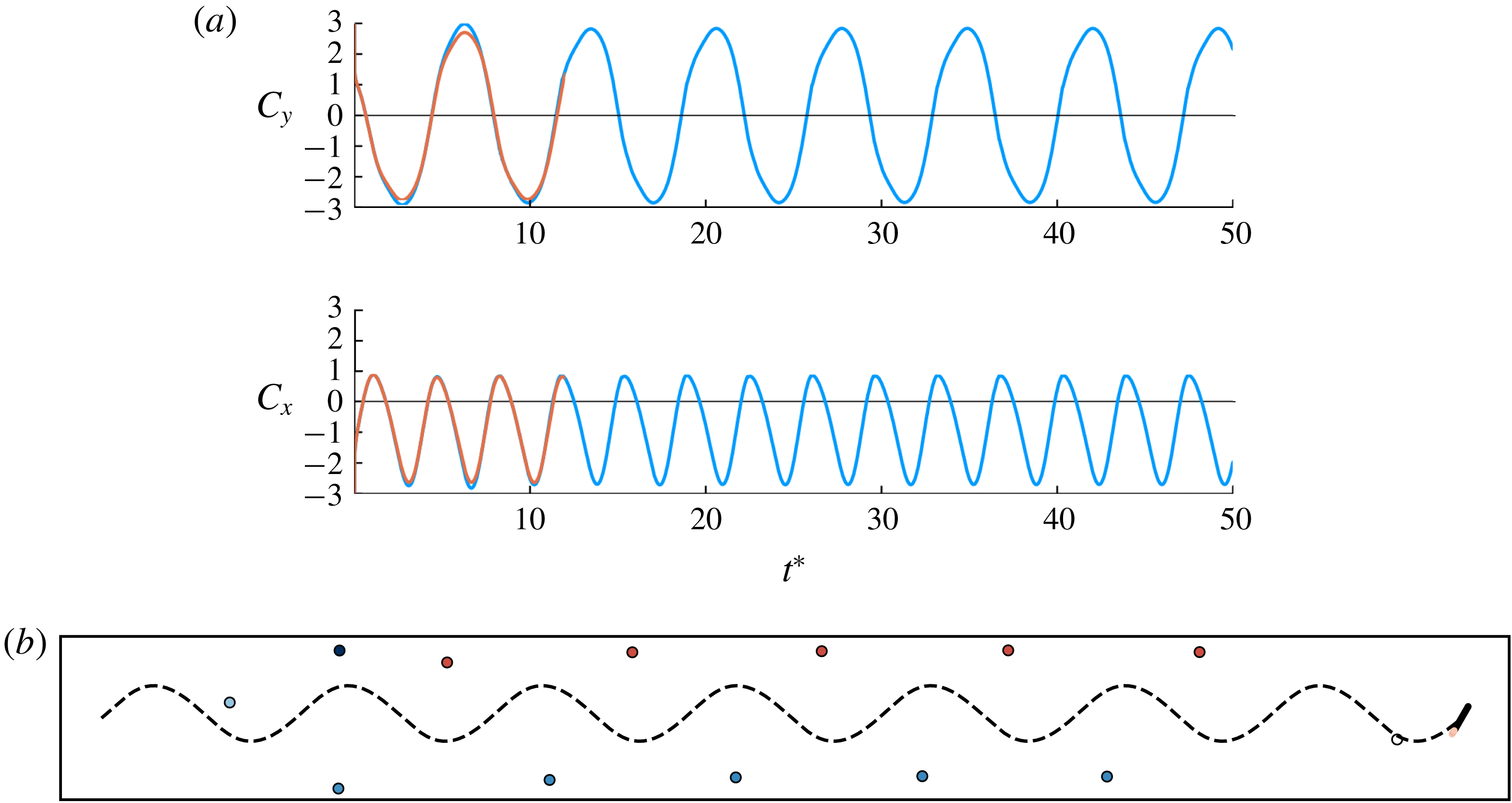
(a) Comparison of the force coefficients generated by oscillatory pitching and heaving at reduced frequency $\unicode[STIX]{x1D705}=0.44$ , heave amplitude $h_{0}/c=1$ and pitch amplitude $\unicode[STIX]{x1D6FC}_{0}=20^{\circ }$ (feathering parameter $\unicode[STIX]{x1D712}=0.48$ ), predicted with hybrid method with $T_{min}^{\ast }=0.2$ and $B_{F}=10^{-1}$ (blue) and full vortex sheet (orange). (b) Snapshot of vorticity from hybrid model at $t^{\ast }=50$ . Trajectory of plate centroid depicted as dashed line. Point vortices coloured blue have clockwise strength, and those in red have anticlockwise strength.

4 Conclusion

In this work, we have developed and demonstrated a hybrid vortex sheet/point vortex model for modelling unsteady separated flows. The parameters of the model – the threshold for force error, $B_{F}$ , and the minimum time between the release of new active vortex elements, $T_{min}^{\ast }$ – can be independently chosen to obtain a rich taxonomy of vortex element models, in which existing models are particular cases. Applying the model to impulsive translation and to pitch-up, we found good agreement with high-fidelity simulations in both the early-time predicted vorticity distribution and the force response. We have also found good quantitative agreement with the theoretical prediction for small-amplitude oscillatory pitching and heaving, and the correct qualitative behaviour for larger amplitudes of this motion. It should be noted that, although we have focused our attention on a thin flat plate in this paper, the proposed methodology would work for any airfoil shape and requires only an expression for the airfoil’s contribution to the impulse of a vortex element in order to compute the velocity correction. The methodology could, in principle, be extended to multiple bodies, though the impulse calculation must then account for all bodies’ contributions.

It should be emphasized that the range of models obtained in this paper share the same well-known challenges with other inviscid models in predicting behaviours that are essentially viscous. This is particularly true for cases in which the flow is expected to separate from the leading edge. By significantly reducing the number of vortex elements in the model, we were able to predict self-sustaining vortex shedding past plates at various angles of attack at a small fraction of the expense of a full discrete vortex element or vortex sheet model. However, the predicted shedding frequency is lower than that observed experimentally or in viscous simulations, indicating that viscosity plays an essential role in establishing this frequency – presumably through the induction of secondary vorticity on the plate and the thickening of the shear layers that roll up into the vortex structures from each edge. In oscillatory pitching and heaving, the vorticity shed from the leading edge, and its subsequent interaction with the trailing-edge structures, can play an important dynamical role, and the models described here are not generally able to predict these dynamics. Fortunately, the low dimensionality of the model opens up the possibility of using data-driven methods to compensate for missing flow physics. Our ongoing work in this area focuses on incorporating data assimilation techniques to use the vortex model as a means for real-time flow estimation.

Acknowledgement

Support by the US Air Force Office of Scientific Research (FA9550-14-1-0328) with programme manager Dr Douglas Smith is gratefully acknowledged.

Appendix A. Derivation of the velocity correction

In this appendix, we first find the expression for the impulse of a point vortex and its associated bound vortex sheet, then we derive the velocity correction for transferring circulation between two point vortices. We make use of a normalized plate-centred coordinate system $(\tilde{x},{\tilde{y}})$ , so that any point can be described by

(A 1)

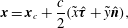$$\begin{eqnarray}\displaystyle \boldsymbol{x}=\boldsymbol{x}_{c}+\frac{c}{2}(\tilde{x}\hat{\unicode[STIX]{x1D749}}+{\tilde{y}}\hat{\boldsymbol{n}}), & & \displaystyle\end{eqnarray}$$

where $c$ is the length of the plate, $\hat{\unicode[STIX]{x1D749}}$ is the unit plate tangent and $\hat{\boldsymbol{n}}$ is the unit plate normal; $\unicode[STIX]{x1D6FC}$ denotes the angle between $\hat{\unicode[STIX]{x1D749}}$ and the positive $x$ axis in the inertial coordinate system. For points that lie on the plate itself, $\tilde{x}$ takes values between $-1$ (at the trailing edge) and $+1$ (at the leading edge), and ${\tilde{y}}$ is identically zero. We will denote the vector position of such points on the plate by $\unicode[STIX]{x1D743}$ . The plate’s motion is completely described by the translational velocity of the centroid, $\dot{\boldsymbol{x}}_{c}$ , and the angular velocity, $\dot{\unicode[STIX]{x1D6FC}}$ .

The impulse of the $i$ th point vortex in the fluid then takes the form

(A 2)

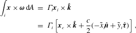$$\begin{eqnarray}\displaystyle \int _{i}\boldsymbol{x}\times \unicode[STIX]{x1D74E}\,\text{d}A & = & \displaystyle \unicode[STIX]{x1D6E4}_{i}\boldsymbol{x}_{i}\times \hat{\boldsymbol{k}}\nonumber\\ \displaystyle & = & \displaystyle \unicode[STIX]{x1D6E4}_{i}\left[\boldsymbol{x}_{c}\times \hat{\boldsymbol{k}}+\frac{c}{2}(-\tilde{x}_{i}\hat{\boldsymbol{n}}+{\tilde{y}}_{i}\hat{\unicode[STIX]{x1D749}})\right],\end{eqnarray}$$

where $\hat{\boldsymbol{k}}$ is the unit vector out of the plate. In order to find the impulse of the bound vortex sheet, we first need the expression for the bound vortex sheet strength.

A.1 Bound vortex sheet strength

The strength of the bound vortex sheet, parametrized by the scaled coordinate along the plate, is denoted by $\unicode[STIX]{x1D6FE}(\tilde{x})$ and is governed by the following integral equation (also known as the airfoil equation):

(A 3)

$$\begin{eqnarray}\displaystyle \frac{1}{2\unicode[STIX]{x03C0}}\int _{-1}^{1}\frac{\unicode[STIX]{x1D6FE}(\unicode[STIX]{x1D70E})}{\tilde{x}-\unicode[STIX]{x1D70E}}\,\text{d}\unicode[STIX]{x1D70E}=\hat{\boldsymbol{n}}\boldsymbol{\cdot }[\boldsymbol{u}_{B}(\unicode[STIX]{x1D743}(\tilde{x}))-\boldsymbol{u}_{A}(\unicode[STIX]{x1D743}(\tilde{x}))], & & \displaystyle\end{eqnarray}$$

where $\tilde{x}\in [-1,1]$ , $\boldsymbol{u}_{B}$ is the velocity of the plate and $\boldsymbol{u}_{A}$ is the velocity induced by ambient vorticity; uniform flow is absent, since we set the problem in a frame of reference in which the fluid is at rest at infinity. We can solve (A 3) using an inversion formula found in Muskhelishvili (Reference Muskhelishvili2013) to find that

(A 4)

$$\begin{eqnarray}\displaystyle \unicode[STIX]{x1D6FE}(\tilde{x})=\frac{2}{\unicode[STIX]{x03C0}\sqrt{1-\tilde{x}^{2}}}\left(\frac{\unicode[STIX]{x1D6E4}_{A}}{c}+\int _{-1}^{1}\frac{\sqrt{1-\unicode[STIX]{x1D70E}^{2}}}{\unicode[STIX]{x1D70E}-\tilde{x}}\,\hat{\boldsymbol{n}}\boldsymbol{\cdot }[\boldsymbol{u}_{B}(\unicode[STIX]{x1D743}(\unicode[STIX]{x1D70E}))-\boldsymbol{u}_{A}(\unicode[STIX]{x1D743}(\unicode[STIX]{x1D70E}))]\,\text{d}\unicode[STIX]{x1D70E}\right), & & \displaystyle\end{eqnarray}$$

where $\unicode[STIX]{x1D6E4}_{A}$ is the total circulation of the ambient vorticity. As in the work by Jones (Reference Jones2003), we represent $\boldsymbol{u}_{B}$ and $\boldsymbol{u}_{A}$ in the Chebyshev expansions:

(A 5)

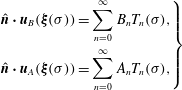$$\begin{eqnarray}\displaystyle \left.\begin{array}{@{}c@{}}\displaystyle \hat{\boldsymbol{n}}\boldsymbol{\cdot }\boldsymbol{u}_{B}(\unicode[STIX]{x1D743}(\unicode[STIX]{x1D70E}))=\mathop{\sum }_{n=0}^{\infty }B_{n}T_{n}(\unicode[STIX]{x1D70E}),\\ \displaystyle \hat{\boldsymbol{n}}\boldsymbol{\cdot }\boldsymbol{u}_{A}(\unicode[STIX]{x1D743}(\unicode[STIX]{x1D70E}))=\mathop{\sum }_{n=0}^{\infty }A_{n}T_{n}(\unicode[STIX]{x1D70E}),\end{array}\right\} & & \displaystyle\end{eqnarray}$$

where $T_{n}(\unicode[STIX]{x1D70E}):=\cos (n\cos ^{-1}\unicode[STIX]{x1D70E})$ is the $n$ th-order Chebyshev polynomial of the first kind. For the rigid plate, $B_{0}=\hat{\boldsymbol{n}}\boldsymbol{\cdot }\dot{\boldsymbol{x}}_{c}$ , $B_{1}=\dot{\unicode[STIX]{x1D6FC}}c/2$ and $B_{n}=0$ for $n>1$ . Substituting these expansions and evaluating the resulting integrals allows us to obtain

(A 6)

$$\begin{eqnarray}\displaystyle \unicode[STIX]{x1D6FE}(\tilde{x})=\frac{2(A_{0}-\hat{\boldsymbol{n}}\boldsymbol{\cdot }\dot{\boldsymbol{x}}_{c})\tilde{x}+A_{1}-c\dot{\unicode[STIX]{x1D6FC}}/2-2\unicode[STIX]{x1D6E4}_{A}/(\unicode[STIX]{x03C0}c)}{\sqrt{1-\tilde{x}^{2}}}-\sqrt{1-\tilde{x}^{2}}\left(\!-c\dot{\unicode[STIX]{x1D6FC}}+2\mathop{\sum }_{n=1}^{\infty }A_{n}U_{n-1}(\tilde{x})\!\right)\!, & & \displaystyle \nonumber\\ \displaystyle & & \displaystyle\end{eqnarray}$$

where $U_{n}(\unicode[STIX]{x1D70E}):=\sin ((n+1)\cos ^{-1}\unicode[STIX]{x1D70E})/\sin (\cos ^{-1}\unicode[STIX]{x1D70E})$ is the $n$ th-order Chebyshev function of the second kind.

As mentioned in § 2, we can decompose (A 6) into contributions from each vortex element, and the contribution from only body motion, i.e. $\unicode[STIX]{x1D6FE}=\sum _{i=1}^{N_{v}}\unicode[STIX]{x1D6FE}_{i}+\unicode[STIX]{x1D6FE}_{B}$ . The coefficients $A_{n}$ , which describe the velocity induced on the plate by these vortex elements, as well as the total circulation of these elements, $\unicode[STIX]{x1D6E4}_{A}$ , can also be decomposed, so that we obtain

(A 7)

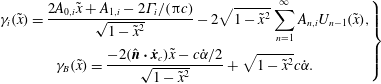$$\begin{eqnarray}\displaystyle \left.\begin{array}{@{}c@{}}\displaystyle \unicode[STIX]{x1D6FE}_{i}(\tilde{x})=\frac{2A_{0,i}\tilde{x}+A_{1,i}-2\unicode[STIX]{x1D6E4}_{i}/(\unicode[STIX]{x03C0}c)}{\sqrt{1-\tilde{x}^{2}}}-2\sqrt{1-\tilde{x}^{2}}\mathop{\sum }_{n=1}^{\infty }A_{n,i}U_{n-1}(\tilde{x}),\\ \displaystyle \unicode[STIX]{x1D6FE}_{B}(\tilde{x})=\frac{-2(\hat{\boldsymbol{n}}\boldsymbol{\cdot }\dot{\boldsymbol{x}}_{c})\tilde{x}-c\dot{\unicode[STIX]{x1D6FC}}/2}{\sqrt{1-\tilde{x}^{2}}}+\sqrt{1-\tilde{x}^{2}}c\dot{\unicode[STIX]{x1D6FC}}.\end{array}\right\} & & \displaystyle\end{eqnarray}$$

We see that the bound vortex sheet strength has square root singularities at the edges of the plate, where $\tilde{x}=\pm 1$ . These singularities form because the plate is infinitely thin and cannot support flow around its edges without an infinite velocity. Noting that real airfoils can support non-zero suction at their leading edges, Ramesh et al. (Reference Ramesh, Gopalarathnam, Granlund, Ol and Edwards2014) proposed a vortex shedding criterion where new vortex elements are released so that the leading-edge suction parameter (LESP), defined as

(A 8)

$$\begin{eqnarray}\displaystyle \text{LESP}:=\frac{1}{2\sqrt{2}U}\lim _{\tilde{x}\rightarrow 1}\unicode[STIX]{x1D6FE}(\tilde{x})\sqrt{1-\tilde{x}}, & & \displaystyle\end{eqnarray}$$

is kept below a critical threshold. Note that the LESP is normalized by the translational speed of the plate, $U=|\dot{\boldsymbol{x}}_{c}|$ . Similarly, the Kutta condition is enforced at the trailing edge by setting

(A 9)

$$\begin{eqnarray}\displaystyle \lim _{\tilde{x}\rightarrow -1}\unicode[STIX]{x1D6FE}(\tilde{x})\sqrt{1+\tilde{x}}=0. & & \displaystyle\end{eqnarray}$$

Substituting expression (A 6) for the bound vortex sheet into the definitions above and combining them, we find that

(A 10)

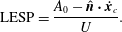$$\begin{eqnarray}\displaystyle \text{LESP}=\frac{A_{0}-\hat{\boldsymbol{n}}\boldsymbol{\cdot }\dot{\boldsymbol{x}}_{c}}{U}. & & \displaystyle\end{eqnarray}$$

A.2 Impulse of the bound vortex sheet

The impulse of a bound vortex sheet on the plate is defined by the integral

(A 11)

$$\begin{eqnarray}\displaystyle \int \unicode[STIX]{x1D6FE}(\boldsymbol{x}\times \hat{\boldsymbol{k}})\,\text{d}l. & & \displaystyle\end{eqnarray}$$

If we substitute the bound vortex sheet strength found in (A 7) and evaluate the resulting integral, we find that the impulse of the bound vortex sheet associated with the $i$ th vortex element is

(A 12)

$$\begin{eqnarray}\displaystyle \oint \unicode[STIX]{x1D6FE}_{i}(\boldsymbol{x}_{i}\times \hat{\boldsymbol{k}})\,\text{d}l=-(\boldsymbol{x}_{c}\times \hat{\boldsymbol{k}})\unicode[STIX]{x1D6E4}_{i}+\hat{\boldsymbol{n}}\unicode[STIX]{x03C0}\left(\frac{c}{2}\right)^{2}\left(A_{0,i}-\frac{A_{2,i}}{2}\right). & & \displaystyle\end{eqnarray}$$

The velocity induced by the $i$ th point vortex at a point $\unicode[STIX]{x1D743}(\unicode[STIX]{x1D70E})$ on the plate can be expressed as

(A 13)

$$\begin{eqnarray}\displaystyle \hat{\boldsymbol{n}}\boldsymbol{\cdot }\boldsymbol{u}_{i}(\unicode[STIX]{x1D743}(\unicode[STIX]{x1D70E}))=\hat{\boldsymbol{n}}\boldsymbol{\cdot }\frac{\unicode[STIX]{x1D6E4}_{i}}{c\unicode[STIX]{x03C0}}\hat{\boldsymbol{k}}\times \frac{(\unicode[STIX]{x1D70E}-\tilde{x}_{i})\hat{\unicode[STIX]{x1D749}}-{\tilde{y}}_{i}\hat{\boldsymbol{n}}}{|(\unicode[STIX]{x1D70E}-\tilde{x}_{i})\hat{\unicode[STIX]{x1D749}}-{\tilde{y}}_{i}\hat{\boldsymbol{n}}|^{2}}=\frac{\unicode[STIX]{x1D6E4}_{i}}{c\unicode[STIX]{x03C0}}\left[\frac{\unicode[STIX]{x1D70E}-\tilde{x}_{i}}{(\unicode[STIX]{x1D70E}-\tilde{x}_{i})^{2}+{\tilde{y}}_{i}^{2}}\right]. & & \displaystyle\end{eqnarray}$$

So the Chebyshev coefficients in (A 12) are given by

(A 14)

$$\begin{eqnarray}\displaystyle A_{0,i}-\frac{A_{2,i}}{2}=\frac{2\unicode[STIX]{x1D6E4}_{i}}{\unicode[STIX]{x03C0}^{2}c}\int _{-1}^{1}\frac{\sqrt{1-\unicode[STIX]{x1D70E}^{2}}}{(\unicode[STIX]{x1D70E}-\tilde{x}_{i})^{2}+{\tilde{y}}_{i}^{2}}(\unicode[STIX]{x1D70E}-\tilde{x}_{i})\,\text{d}\unicode[STIX]{x1D70E}. & & \displaystyle\end{eqnarray}$$

If we define $\tilde{z}_{i}:=\tilde{x}_{i}+\text{i}{\tilde{y}}_{i}$ , then applying contour integration to the integral above gives us

(A 15)

$$\begin{eqnarray}\displaystyle A_{0,i}-\frac{A_{2,i}}{2}=\frac{2\unicode[STIX]{x1D6E4}_{i}}{\unicode[STIX]{x03C0}c}\,\text{Re}\{\tilde{z}_{i}-\sqrt{\tilde{z}_{i}-1}\,\sqrt{\tilde{z}_{i}+1}\}. & & \displaystyle\end{eqnarray}$$

Combining (A 2), (A 12) and (A 15), we find that the impulse of a point vortex and its bound vortex sheet is given by

(A 16)

$$\begin{eqnarray}\displaystyle \boldsymbol{P}=\unicode[STIX]{x1D6E4}_{i}\frac{c}{2}[\hat{\unicode[STIX]{x1D749}}\,\text{Im}\{\tilde{z}_{i}\}-\hat{\boldsymbol{n}}\,\text{Re}\{\sqrt{\tilde{z}_{i}-1}\,\sqrt{\tilde{z}_{i}+1}\}]. & & \displaystyle\end{eqnarray}$$

A.3 Velocity correction

To streamline the derivation of the velocity correction, we will use the complex form of (A 16), and omit the subscript $i$ for brevity:

(A 17)

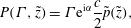$$\begin{eqnarray}\displaystyle P(\unicode[STIX]{x1D6E4},\tilde{z})=\unicode[STIX]{x1D6E4}\text{e}^{\text{i}\unicode[STIX]{x1D6FC}}\frac{c}{2}\tilde{p}(\tilde{z}), & & \displaystyle\end{eqnarray}$$

where $\tilde{p}$ is defined as

(A 18)

$$\begin{eqnarray}\displaystyle \tilde{p}(\tilde{z}):=\text{Im}\{\tilde{z}\}-\text{i}\,\text{Re}\{\sqrt{\tilde{z}-1}\,\sqrt{\tilde{z}+1}\}. & & \displaystyle\end{eqnarray}$$

The time derivative of the impulse is then given by

(A 19)

$$\begin{eqnarray}\displaystyle \frac{\text{d}P}{\text{d}t}(\unicode[STIX]{x1D6E4},\tilde{z})=\text{i}\dot{\unicode[STIX]{x1D6FC}}P(\unicode[STIX]{x1D6E4},\tilde{z})+\text{e}^{\text{i}\unicode[STIX]{x1D6FC}}\frac{c}{2}\left[\dot{\unicode[STIX]{x1D6E4}}\tilde{p}(\tilde{z})+\unicode[STIX]{x1D6E4}\frac{\text{d}\tilde{p}}{\text{d}t}(\tilde{z})\right], & & \displaystyle\end{eqnarray}$$

where

(A 20)

$$\begin{eqnarray}\displaystyle \frac{\text{d}\tilde{p}}{\text{d}t}(\tilde{z})=-\text{i}\left[\dot{\tilde{z}}+\text{Re}\left\{\left(\frac{\tilde{z}}{\sqrt{\tilde{z}-1}\,\sqrt{\tilde{z}+1}}-1\right)\dot{\tilde{z}}\right\}\right]. & & \displaystyle\end{eqnarray}$$

As before, we will use the subscripts $s$ and $t$ to refer to the point vortices we are transferring circulation from and to, respectively, and $\dot{\unicode[STIX]{x1D6E4}}$ to represent the rate at which circulation is gained by the target $t$ (and simultaneously lost by the source $s$ ). The rate of change of impulse due to these two point vortices, including the effect of circulation transfer, is

(A 21)

$$\begin{eqnarray}\displaystyle \frac{\text{d}P_{s}}{\text{d}t}+\frac{\text{d}P_{t}}{\text{d}t}=\text{i}\dot{\unicode[STIX]{x1D6FC}}(P_{s}+P_{t})+\text{e}^{\text{i}\unicode[STIX]{x1D6FC}}\frac{c}{2}\left[\dot{\unicode[STIX]{x1D6E4}}(\tilde{p}_{t}-\tilde{p}_{s})+\unicode[STIX]{x1D6E4}_{s}\frac{\text{d}\tilde{p}_{s}}{\text{d}t}+\unicode[STIX]{x1D6E4}_{t}\left(\frac{\text{d}\tilde{p}_{t}}{\text{d}t}+\frac{\text{d}\unicode[STIX]{x0394}\tilde{p}_{t}}{\text{d}t}\right)\right],\qquad & & \displaystyle\end{eqnarray}$$

where $\text{d}\unicode[STIX]{x0394}\tilde{p}_{t}/\text{d}t$ comes from applying a velocity correction to the target point vortex. The first term in square brackets represents the spurious force arising from the transfer of circulation. For the velocity correction to cancel out the effect of changing circulation, we must have

(A 22)

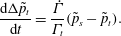$$\begin{eqnarray}\displaystyle \frac{\text{d}\unicode[STIX]{x0394}\tilde{p}_{t}}{\text{d}t}=\frac{\dot{\unicode[STIX]{x1D6E4}}}{\unicode[STIX]{x1D6E4}_{t}}(\tilde{p}_{s}-\tilde{p}_{t}). & & \displaystyle\end{eqnarray}$$

If we define

(A 23)

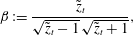$$\begin{eqnarray}\displaystyle \unicode[STIX]{x1D6FD}:=\frac{\tilde{z}_{t}}{\sqrt{\tilde{z}_{t}-1}\,\sqrt{\tilde{z}_{t}+1}}, & & \displaystyle\end{eqnarray}$$

then we can combine (A 22) and (A 20) to get

(A 24)

$$\begin{eqnarray}\displaystyle \unicode[STIX]{x0394}\dot{\tilde{z}}_{t}(\unicode[STIX]{x1D6FD}+1)+\unicode[STIX]{x0394}\dot{\tilde{z}}_{t}^{\star }(\unicode[STIX]{x1D6FD}^{\star }-1)=2\text{i}\frac{\dot{\unicode[STIX]{x1D6E4}}}{\unicode[STIX]{x1D6E4}_{t}}(\tilde{p}_{s}-\tilde{p}_{t}). & & \displaystyle\end{eqnarray}$$

We can combine this equation with its conjugate,

(A 25)

$$\begin{eqnarray}\displaystyle \unicode[STIX]{x0394}\dot{\tilde{z}}_{t}^{\star }(\unicode[STIX]{x1D6FD}^{\star }+1)+\unicode[STIX]{x0394}\dot{\tilde{z}}_{t}(\unicode[STIX]{x1D6FD}-1)=-2\text{i}\frac{\dot{\unicode[STIX]{x1D6E4}}}{\unicode[STIX]{x1D6E4}_{t}}(\tilde{p}_{s}^{\star }-\tilde{p}_{t}^{\star }), & & \displaystyle\end{eqnarray}$$

to obtain the velocity correction to the target point vortex,

(A 26)

$$\begin{eqnarray}\displaystyle \unicode[STIX]{x0394}{\dot{z}}_{t}=\frac{\text{e}^{\text{i}\unicode[STIX]{x1D6FC}}c}{2}\unicode[STIX]{x0394}\dot{\tilde{z}}_{t}=\frac{\text{i}\text{e}^{\text{i}\unicode[STIX]{x1D6FC}}c}{2}\frac{\dot{\unicode[STIX]{x1D6E4}}}{\unicode[STIX]{x1D6E4}_{t}}\left(\frac{(\tilde{p}_{s}-\tilde{p}_{t})(\unicode[STIX]{x1D6FD}^{\star }+1)+(\tilde{p}_{s}^{\star }-\tilde{p}_{t}^{\star })(\unicode[STIX]{x1D6FD}^{\star }-1)}{\unicode[STIX]{x1D6FD}+\unicode[STIX]{x1D6FD}^{\star }}\right). & & \displaystyle\end{eqnarray}$$

References

Alben, S. & Shelley, M. J. 2008 Flapping states of a flag in an inviscid fluid: bistability and the transition to chaos. Phys. Rev. Lett. 100 (7), 074301.Google Scholar

Anderson, J. M., Streitlien, K., Barrett, D. S. & Triantafyllou, M. S. 1998 Oscillating foils of high propulsive efficiency. J. Fluid Mech. 360, 41–72.Google Scholar

Ansari, S. A., Zbikowski, R. & Knowles, K. 2006 Non-linear unsteady aerodynamic model for insect-like flapping wings in the hover. Part 2: Implementation and validation. Proc. Inst. Mech. Engrs 220, 169–186.Google Scholar

Birch, J. M. & Dickinson, M. H. 2001 Spanwise flow and the attachment of the leading-edge vortex on insect wings. Nature 412 (6848), 729–733.Google Scholar

Brown, C. E. & Michael, W. H. 1954 Effect of leading-edge separation on the lift of a delta wing. J. Aero. Sci. 21 (10), 690–694.Google Scholar

Chorin, A. J. 1990 Hairpin removal in vortex interactions. J. Comput. Phys. 91 (1), 1–21.Google Scholar

Dickinson, M. H. & Götz, K. 1993 Unsteady aerodynamic performance of model wings at low Reynolds numbers. J. Exp. Biol. 174, 45–64.Google Scholar

Eldredge, J. D., Wang, C. & Ol, M. V.2009 A computational study of a canonical pitch-up, pitch-down wing maneuver. In 39th AIAA Fluid Dynamics Conference. AIAA Paper 2009-3687.Google Scholar

Fage, A. & Johansen, F. C. 1927 On the flow of air behind an inclined plate of infinite span. Proc. R. Soc. Lond. A 116 (773), 170–197.Google Scholar

Greengard, L. & Rokhlin, V. 1987 A fast algorithm for particle simulations. J. Comput. Phys. 73 (2), 325–348.Google Scholar

Jones, M. A. 2003 The separated flow of an inviscid fluid around a moving flat plate. J. Fluid Mech. 496, 405–441.Google Scholar

von Kármán, T. & Sears, W. R. 1938 Airfoil theory for non-uniform motion. J. Aero. Sci. 5 (10), 379–390.Google Scholar

Katz, J. 1981 A discrete vortex method for the non-steady separated flow over an airfoil. J. Fluid Mech. 102, 315–328.Google Scholar

Kinsey, T. & Dumas, G. 2008 Parametric study of an oscillating airfoil in a power-extraction regime. AIAA J. 46 (6), 1318–1330.Google Scholar

Krasny, R. 1986 A study of singularity formation in a vortex sheet by the point-vortex approximation. J. Fluid Mech. 167, 65–93.Google Scholar

Krasny, R. & Nitsche, M. 2002 The onset of chaos in vortex sheet flow. J. Fluid Mech. 454, 47–69.Google Scholar

Li, J. & Wu, Z.-N. 2016 A vortex force study for a flat plate at high angle of attack. J. Fluid Mech. 801, 222–249.Google Scholar

Michelin, S. & Llewellyn Smith, S. G. 2009 An unsteady point vortex method for coupled fluid–solid problems. Theor. Comput. Fluid Dyn. 23, 127–153.Google Scholar

Moore, D. 1979 The spontaneous appearance of a singularity in the shape of an evolving vortex sheet. Proc. R. Soc. Lond. A 365 (1720), 105–119.Google Scholar

Muskhelishvili, N. 2013 Singular Integral Equations, Boundary Problems of Function Theory and Their Application to Mathematical Physics. Dover Publications; corrected reprint of the Noordhoff translation (1953) of the Russian original of 1946.Google Scholar

Nitsche, M., Taylor, M. A. & Krasny, R. 2003 Comparison of regularizations of vortex sheet motion. In Computational Fluid and Solid Mechanics, pp. 1062–1065. Elsevier.Google Scholar

Pullin, D. I. 1978 The large-scale structure of unsteady self-similar rolled-up vortex sheets. J. Fluid Mech. 88 (03), 401–430.Google Scholar

Ramesh, K., Gopalarathnam, A., Edwards, J. R., Ol, M. V. & Granlund, K. 2013 An unsteady airfoil theory applied to pitching motions validated against experiment and computation. Theor. Comput. Fluid Dyn. 27 (6), 843–864.Google Scholar

Ramesh, K., Gopalarathnam, A., Granlund, K., Ol, M. V. & Edwards, J. R. 2014 Discrete-vortex method with novel shedding criterion for unsteady aerofoil flows with intermittent leading-edge vortex shedding. J. Fluid Mech. 751, 500–548.Google Scholar

Rossi, L. F. 1997 Merging computational elements in vortex simulations. SIAM J. Sci. Comput. 18 (4), 1014–1027.Google Scholar

Sarpkaya, T. 1975 An inviscid model of two-dimensional vortex shedding for transient and asymptotically steady separated flow over an inclined plate. J. Fluid Mech. 68, 109–128.Google Scholar

Shukla, R. K. & Eldredge, J. D. 2007 An inviscid model for vortex shedding from a deforming body. Theor. Comput. Fluid Dyn. 21 (5), 343–368.Google Scholar

Taira, K. & Colonius, T. 2007 The immersed boundary method: a projection approach. J. Comput. Phys. 225 (2), 2118–2137.Google Scholar

Taira, K., Dickson, W. B., Colonius, T. & Dickinson, M. H.2007 Unsteadiness in flow over a flat plate at angle-of-attack at low Reynolds numbers. In 45th AIAA Aerosp. Sci. Meet. Exhib. AIAA Paper 2007-0710.Google Scholar

Tchieu, A. & Leonard, A. 2011 A discrete-vortex model for the arbitrary motion of a thin airfoil with fluidic control. J. Fluids Struct. 27 (5–6), 680–693.Google Scholar

Theodorsen, T.1935 General theory of aerodynamic instability and the mechanism of flutter. NACA Tech. Rep. TR-496.Google Scholar

Wagner, H. 1925 Über die Entstehung des dynamischen Auftriebes von Tragflügeln. Z. Angew. Math. Mech. 5 (1), 17–35.Google Scholar

Wang, C. & Eldredge, J. D. 2013 Low-order phenomenological modeling of leading-edge vortex formation. Theor. Comput. Fluid Dyn. 27 (5), 577–598.Google Scholar

Xia, X. & Mohseni, K. 2013 Lift evaluation of a two-dimensional pitching flat plate. Phys. Fluids 25 (9), 091901.Google Scholar

Figure 1.The model: $\boldsymbol{x}_{c}$, $\unicode[STIX]{x1D6FC}$ and $c$ denote the centroid, angle of attack and chord length of the plate. Each vortex sheet has an associated point vortex that it feeds circulation into.

Figure 2.Taxonomy of vortex element models. Comparison of the vorticity distribution predicted by the hybrid model at limiting values of the tolerance for force error, $B_{F}$, and the minimum vortex release interval, $T_{min}$.

Figure 3.CPU time required in each time step versus the number of total vortex elements in the problem: for velocity induction and advection (●, blue), Kutta condition enforcement (▪, green), and circulation transfer procedures and sheet filtering (●, red-brown). Results generated from the simulation of an impulsively started plate at $45^{\circ }$ angle of attack.

Figure 4.Comparison of the vorticity distribution predicted for a flat plate moved impulsively at $45^{\circ }$ after one (a,c,e) and three (b,d,f) chord lengths of travel between the new hybrid model with $T_{min}^{\ast }=0.2$ (a,b), a full vortex sheet model (c,d) and a high-fidelity simulation at $Re=500$ (e,f). The positions of the positive- and negative-strength point vortices are shown with filled and unfilled circles, respectively, and $N$ denotes the total number of vortex elements (including those in the vortex sheets).

Figure 5.Number of vortex elements (a) and cumulative CPU time (b) of the hybrid model with $T_{min}^{\ast }=0.2$ (– –) and the vortex sheet model (- - - -), for impulsive translation at $\unicode[STIX]{x1D6FC}=45^{\circ }$.

Figure 6.Early-time lift (a) and drag (b) coefficients for impulsive translation at $\unicode[STIX]{x1D6FC}=45^{\circ }$ predicted by the hybrid model with $T_{min}^{\ast }=0.2$ (– –), the vortex sheet model (- - - -), the Wang & Eldredge model (– ⋅ – ⋅) and high-fidelity simulation at $Re=500$ (——).

Figure 7.Comparison of the vorticity distribution in a hybrid model of flow around an impulsively translated plate with $\unicode[STIX]{x1D6FC}=45^{\circ }$ at $t^{\ast }=10$, using three different choices for minimum time between initiation of new active vortex elements, $T_{min}^{\ast }$.

Figure 8.Comparison of the number of vortex elements used over time to simulate impulsive translation at $45^{\circ }$, using different values of minimum vortex release time interval: $T_{min}^{\ast }=0.1$ (——, red), $T_{min}^{\ast }=0.2$ (——, black) and $T_{min}^{\ast }=0.25$ (– ⋅ – ⋅, green).

Figure 9.Lift (a) and drag (b) coefficients for impulsive translation at $\unicode[STIX]{x1D6FC}=45^{\circ }$ predicted by the hybrid model with $T_{min}^{\ast }=0.1$ (——, red), $T_{min}^{\ast }=0.2$ (——, black) and $T_{min}^{\ast }=0.25$ (– – –, green).

Figure 10.Comparison of the vorticity distribution predicted for a flat plate moved impulsively at $60^{\circ }$ at three different instants between the new hybrid model with $T_{min}^{\ast }=0.2$ (a–c), a full vortex sheet model (d–f) and high-fidelity simulation at $Re=500$ (g–i). The positions of the positive- and negative-strength point vortices are shown with filled and unfilled circles, respectively, and $N$ denotes the total number of vortex elements (including those in the vortex sheets).

Figure 11.Early-time lift (a) and drag (b) coefficients for impulsive translation at $\unicode[STIX]{x1D6FC}=60^{\circ }$ predicted by the hybrid model with $T_{min}^{\ast }=0.2$ (– –), the vortex sheet model (- - - -), the Wang & Eldredge model (– ⋅ – ⋅) and the high-fidelity simulation at $Re=500$ (——).

Figure 12.Lift (a) and drag (b) coefficients for impulsive translation at $\unicode[STIX]{x1D6FC}=60^{\circ }$ predicted by the hybrid model with $T_{min}^{\ast }=0.1$ (——, red), $T_{min}^{\ast }=0.2$ (– ⋅ – ⋅, green) and $T_{min}^{\ast }=0.25$ (– –, blue).

Figure 13.Error versus minimum time between releases of new active point vortices, $T_{min}^{\ast }$, and tolerance for force discrepancy, $B_{F}$, for impulsive translation of a flat plate at $60^{\circ }$ angle of incidence, after four convective time units. Error is defined as the r.m.s. difference in force from a reference case, normalized by the $L_{2}$ norm of the reference case force. The reference case is a full vortex sheet, generated with $T_{min}^{\ast }=\infty$ and $B_{F}=0$. The cases shown are: $B_{F}=3\times 10^{-1}$ (blue), $2\times 10^{-1}$ (orange),$10^{-1}$ (green), $6.25\times 10^{-2}$ (purple), $5\times 10^{-2}$ (mustard), $3.5\times 10^{-2}$ (turquoise), $1.25\times 10^{-2}$ (pink) and $6.25\times 10^{-3}$ (brown). The shaded region corresponds to cases with minimal generation of discrete vortex elements. Snapshots of a few sample cases at $t^{\ast }=2.5$, along with the corresponding number of total vortex elements, are shown.

Figure 14.Error (red-brown) and total number of vortex elements (blue) versus tolerance for force discrepancy, $B_{F}$, with minimum release time, $T_{min}^{\ast }$, set to $1$, for impulsive translation of a flat plate at $60^{\circ }$ angle of incidence, after four convective time units. Error is defined as in figure 13.

Figure 15.Early-time moment coefficient (about the centroid) for impulsive translation at $\unicode[STIX]{x1D6FC}=60^{\circ }$ predicted by the hybrid model with $T_{min}^{\ast }=0.2$ and $B_{F}=10^{-1}$ (– –, red), $T_{min}^{\ast }=0.2$ and $B_{F}=5\times 10^{-2}$ (——, green), and the vortex sheet model (- - - -, purple).

Figure 16.Histories of angle of attack of flat plate for pitch-up problem: $K=0.7$ (blue) and $K=0.2$ (red).

Figure 17.Comparison of the vorticity distribution predicted for a flat plate pitching with $K=0.7$ at two different instants between the hybrid model with $T_{min}^{\ast }=0.1$ (a,b) and a high-fidelity simulation at $Re=1000$ (c,d) at $\unicode[STIX]{x1D6FC}=33^{\circ }$ (a,c) and $\unicode[STIX]{x1D6FC}=90^{\circ }$ (b,d).

Figure 18.Early-time lift (a) and drag (b) coefficients for a pitch-up manoeuvre at $K=0.7$ predicted by the hybrid model with $T_{min}^{\ast }=0.1$ (– –, red), the Wang & Eldredge model (– ⋅ – ⋅, green) and high-fidelity simulation results at $Re=1000$ (——, blue).

Figure 19.Comparison of the long-term lift and drag coefficients for a pitch-up manoeuvre at $K=0.7$ predicted with $T_{min}^{\ast }=0.1$ (——, red) and $T_{min}^{\ast }=0.2$ (– –, blue).

Figure 20.Comparison of the vorticity distribution predicted for a flat plate pitching with $K=0.2$ at two different instants between the hybrid model with $T_{min}^{\ast }=0.2$ (a–c) and a high-fidelity simulation at $Re=1000$ (d–f) at $\unicode[STIX]{x1D6FC}=23^{\circ }$ (a,d), $\unicode[STIX]{x1D6FC}=57^{\circ }$ (b,e) and $\unicode[STIX]{x1D6FC}=87^{\circ }$ (c,f).

Figure 21.Early-time lift (a) and drag (b) coefficients for a pitch-up manoeuvre at $K=0.2$ predicted by the hybrid model with $T_{min}^{\ast }=0.2$ (– –, red), the Wang & Eldredge model (– ⋅ – ⋅, green) and high-fidelity simulation results at $Re=1000$ (——, blue).

Figure 22.Comparison of the lift coefficient generated by oscillatory pitching and heaving at reduced frequency $\unicode[STIX]{x1D705}=1$, heave amplitude $h_{0}/c=0.05$ and pitch amplitude $\unicode[STIX]{x1D6FC}_{0}=5^{\circ }$, predicted with $T_{min}^{\ast }=0.1$ (——, blue), $T_{min}^{\ast }=0.4$ (——, red) and full vortex sheet (——, green). The Theodorsen solution (– –) is shown for reference. Both hybrid method results use $B_{F}=1.75\times 10^{-2}$.

Figure 23.Snapshots of the vorticity distribution at $t^{\ast }=25$ generated by oscillatory pitching and heaving at reduced frequency $\unicode[STIX]{x1D705}=1$, heave amplitude $h_{0}/c=0.05$ and pitch amplitude $\unicode[STIX]{x1D6FC}_{0}=5^{\circ }$, predicted with full vortex sheet (a), hybrid model with $T_{min}^{\ast }=0.4$ (b) and hybrid model with $T_{min}^{\ast }=0.1$ (c). Both hybrid method results use $B_{F}=1.75\times 10^{-2}$.

Figure 24.(a) Comparison of the force coefficients generated by oscillatory pitching and heaving at reduced frequency $\unicode[STIX]{x1D705}=0.44$, heave amplitude $h_{0}/c=1$ and pitch amplitude $\unicode[STIX]{x1D6FC}_{0}=60^{\circ }$ (feathering parameter $\unicode[STIX]{x1D712}=1.45$), predicted with hybrid method with $T_{min}^{\ast }=0.2$ and $B_{F}=10^{-1}$ (blue) and full vortex sheet (orange). (b) Snapshot of vorticity from hybrid model at $t^{\ast }=50$. Trajectory of plate centroid depicted as dashed line. Point vortices coloured blue have clockwise strength, and those in red have anticlockwise strength.

Figure 25.(a) Comparison of the force coefficients generated by oscillatory pitching and heaving at reduced frequency $\unicode[STIX]{x1D705}=0.44$, heave amplitude $h_{0}/c=1$ and pitch amplitude $\unicode[STIX]{x1D6FC}_{0}=20^{\circ }$ (feathering parameter $\unicode[STIX]{x1D712}=0.48$), predicted with hybrid method with $T_{min}^{\ast }=0.2$ and $B_{F}=10^{-1}$ (blue) and full vortex sheet (orange). (b) Snapshot of vorticity from hybrid model at $t^{\ast }=50$. Trajectory of plate centroid depicted as dashed line. Point vortices coloured blue have clockwise strength, and those in red have anticlockwise strength.

Article contents

A versatile taxonomy of low-dimensional vortex models for unsteady aerodynamics

Abstract

JFM classification

Information

1 Introduction

2 Model formulation

2.1 Effect of circulation transfer on force

2.2 Impulse matching velocity correction

2.3 Circulation transfer rate

2.4 Regularization and Fourier filtering

2.5 Computational cost

3 Results

3.1 Impulsive translation at fixed angle of attack

3.1.1 Translation at $45^{\circ }$ angle of attack

3.1.2 Translation at $60^{\circ }$ angle of attack

3.2 Pitch-up while translating

3.3 Oscillatory pitching and heaving

4 Conclusion

Acknowledgement

Appendix A. Derivation of the velocity correction

A.1 Bound vortex sheet strength

A.2 Impulse of the bound vortex sheet

A.3 Velocity correction

References

Save article to Kindle

Save article to Dropbox

Save article to Google Drive

Reply to: Submit a response

Your details

You have entered the maximum number of contributors

Conflicting interests