2. Background and notation

Throughout the paper we use the following notation. The symbol ${\textbf{\textit{X}}}\sim N_n({\boldsymbol{\mu}},{\boldsymbol{\Sigma}})$ , ${n\in{\mathbb{N}}}$ , means an n-dimensional random vector that follows a multivariate Gaussian distribution with mean ${\boldsymbol{\mu}}\in{\mathbb{R}}^n$ and positive-definite covariance matrix ${\boldsymbol{\Sigma}}={\boldsymbol{\sigma}}\bar{{\boldsymbol{\Sigma}}}{\boldsymbol{\sigma}}\in {\mathbb{R}}^n\times{\mathbb{R}}^n$ , ${\boldsymbol{\sigma}}\,:\!=\text{diag}(\sigma_{11},\dots,\sigma_{nn})$ ; $\bar{{\boldsymbol{\Sigma}}}$ is the correlation matrix. Its cumulative distribution function (CDF) and probability density function (PDF) are denoted by $\Phi_n({\textbf{\textit{x}}};\,{\boldsymbol{\mu}},{\boldsymbol{\Sigma}})$ and $\phi_n({\textbf{\textit{x}}};\,{\boldsymbol{\mu}},{\boldsymbol{\Sigma}})$ , respectively, with ${\textbf{\textit{x}}}\in{\mathbb{R}}^n$ . When ${\boldsymbol{\mu}}={\textbf{0}}=(0,\ldots,0)^\top$ and ${\boldsymbol{\Sigma}}={\textbf{\textit{I}}}$ , where ${\textbf{\textit{I}}}$ is the identity matrix, we write $\Phi_n({\textbf{\textit{x}}})$ for simplicity. We use the notation 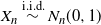$X_n \overset{\text{i.i.d.}}{\sim} N_n(0,1)$ , $n=1,2,\ldots$ , to indicate that $X_1,\ldots,X_n$ are independent and identically distributed (i.i.d.) RVs with distribution N(0,1).

We indicate by $\textbf{1}_{a,b}$ ( ${\textbf{0}}_{a,b}$ ) the matrix of dimension $a\times b$ whose elements are all equal to one (zero). We omit the subscripts when the dimensions of the matrices are clear from the context. Matrices having one subscript are column vectors.

We introduce the notion of a multivariate closed skew-normal (CSN) random vector and we do so by using the so-called conditioning representation [Reference Genton12, Chapter 2]. Let ${\textbf{\textit{U}}}\sim N_m({\boldsymbol{\xi}},{\boldsymbol{\Omega}})$ be independent of ${\textbf{\textit{V}}}\sim N_n({\textbf{0}},{\boldsymbol{\Sigma}})$ , where ${\boldsymbol{\xi}}\in{\mathbb{R}}^m$ , ${\boldsymbol{\Omega}}\in{\mathbb{R}}^m\times {\mathbb{R}}^m$ and ${\boldsymbol{\Sigma}}\in {\mathbb{R}}^n\times {\mathbb{R}}^n$ . Let ${\boldsymbol{\Delta}}\in{\mathbb{R}}^n\times{\mathbb{R}}^m$ ; then

\begin{equation*}\begin{pmatrix}{\textbf{\textit{U}}}\\{\boldsymbol{\Delta}}{\textbf{\textit{U}}}+{\textbf{\textit{V}}}\end{pmatrix}\sim N_{m+n}\left(\begin{pmatrix}{\boldsymbol{\xi}}\\{\boldsymbol{\Delta}}{\boldsymbol{\xi}}\end{pmatrix},\begin{pmatrix}{\boldsymbol{\Omega}\ \ } & {\boldsymbol{\Omega}}{\boldsymbol{\Delta}}^\top\\{\boldsymbol{\Delta}}{\boldsymbol{\Omega}\ \ } & {\boldsymbol{\Gamma}}\end{pmatrix}\right),\end{equation*}

where ${\boldsymbol{\Gamma}} = {\boldsymbol{\Sigma}} + {\boldsymbol{\Delta}}{\boldsymbol{\Omega}}{\boldsymbol{\Delta}}^\top$ . Define ${\textbf{\textit{X}}}$ equal to ${\textbf{\textit{U}}}$ , under the condition that ${\boldsymbol{\Delta}}{\textbf{\textit{U}}}+{\textbf{\textit{V}}} > {\boldsymbol{\mu}}$ , denoted by ${\textbf{\textit{X}}}=({\textbf{\textit{U}}} \mid {\boldsymbol{\Delta}}{\textbf{\textit{U}}}+{\textbf{\textit{V}}} > {\boldsymbol{\mu}})$ , where ${\boldsymbol{\mu}}\in{\mathbb{R}}^n$ . The m-dimensional random vector ${\textbf{\textit{X}}}$ follows a multivariate CSN distribution, ${\textbf{\textit{X}}}\sim \text{CSN}_{m,n}({\boldsymbol{\xi}},{\boldsymbol{\Omega}},{\boldsymbol{\Delta}},{\boldsymbol{\mu}},{\boldsymbol{\Sigma}})$ , whose PDF is, for all ${\textbf{\textit{x}}}\in{\mathbb{R}}^m$ ,

\begin{equation*}\psi_{m,n}({\textbf{\textit{x}}};\,{\boldsymbol{\xi}},{\boldsymbol{\Omega}},{\boldsymbol{\Delta}},{\boldsymbol{\mu}},{\boldsymbol{\Sigma}})=\frac{\phi_m({\textbf{\textit{x}}}-{\boldsymbol{\xi}};\,{\boldsymbol{\Omega}}) \Phi_n({\boldsymbol{\Delta}}({\textbf{\textit{x}}}-{\boldsymbol{\xi}});\,{\boldsymbol{\mu}},{\boldsymbol{\Sigma}})}{\Phi_n({\textbf{0}};\,{\boldsymbol{\mu}},{\boldsymbol{\Gamma}})}.\end{equation*}

We denote the CDF of ${\textbf{\textit{X}}}$ by $\Psi_{m,n}({\textbf{\textit{x}}};\,{\boldsymbol{\xi}},{\boldsymbol{\Omega}},{\boldsymbol{\Delta}},{\boldsymbol{\mu}},{\boldsymbol{\Sigma}})\,:\!=\text{P}({\textbf{\textit{U}}}\leq {\textbf{\textit{x}}} \mid {\boldsymbol{\Delta}}{\textbf{\textit{U}}}+{\textbf{\textit{V}}} > {\boldsymbol{\mu}})$ . When ${\boldsymbol{\xi}}={\textbf{0}}$ , ${\boldsymbol{\Omega}}={\textbf{\textit{I}}}$ and ${\boldsymbol{\mu}}={\textbf{0}}$ , we omit them among the parameters for simplicity and we write $\Psi_{m,n}({\textbf{\textit{x}}};\,{\boldsymbol{\Delta}},{\boldsymbol{\Sigma}})$ and $\psi_{m,n}({\textbf{\textit{x}}};\,{\boldsymbol{\Delta}},{\boldsymbol{\Sigma}})$ instead. We recall that the CSN distribution is also known in the literature as the unified multivariate skew-normal distribution, which simply uses a different parametrisation (e.g. [Reference Azzalini3, Section 7.1.2]). The exposition of our results benefits from the parametrisation used by the CSN distribution.

We recall that if ${\textbf{\textit{X}}}\sim \text{CSN}_{m,n}({\boldsymbol{\xi}},{\boldsymbol{\Omega}},{\boldsymbol{\Delta}},{\boldsymbol{\mu}},{\boldsymbol{\Sigma}})$ then

(1) \begin{equation}\text{P}({\textbf{\textit{U}}}\leq {\textbf{\textit{x}}} \mid {\boldsymbol{\Delta}}{\textbf{\textit{U}}}+{\textbf{\textit{V}}} > {\boldsymbol{\mu}})=\frac{\Phi_{n+m}(\tilde{{\textbf{\textit{x}}}};\,\tilde{{\boldsymbol{\Omega}}})}{\Phi_n({\textbf{0}};\,{\boldsymbol{\mu}},{\boldsymbol{\Gamma}})},\end{equation}

where

\begin{equation*}\tilde{{\textbf{\textit{x}}}}=\begin{pmatrix}-{\boldsymbol{\mu}}\\{\textbf{\textit{x}}}-{\boldsymbol{\xi}}\end{pmatrix},\quad\tilde{{\boldsymbol{\Omega}}}=\begin{pmatrix}{\boldsymbol{\Gamma}} & -{\boldsymbol{\Delta}}{\boldsymbol{\Omega}}\\-{\boldsymbol{\Omega}}{\boldsymbol{\Delta}}^\top & {\boldsymbol{\Omega}}\end{pmatrix}; \end{equation*}

see [Reference Azzalini and Bacchieri4]. Furthermore, for ${\textbf{\textit{b}}}\in {\mathbb{R}}^m$ and ${\textbf{\textit{A}}}\in{\mathbb{R}}^q\times{\mathbb{R}}^m$ ,

(2) \begin{align}{\textbf{\textit{b}}}+{\textbf{\textit{X}}} & \sim \text{CSN}_{m,n}({\boldsymbol{\xi}}+{\textbf{\textit{b}}},{\boldsymbol{\Omega}},{\boldsymbol{\Delta}},{\boldsymbol{\mu}},{\boldsymbol{\Sigma}}) , \nonumber \\{\textbf{\textit{A}}}{\textbf{\textit{X}}} & \sim \text{CSN}_{q,n}({\textbf{\textit{A}}}{\boldsymbol{\xi}},{\boldsymbol{\Omega}}^{*},{\boldsymbol{\Delta}}^*,{\boldsymbol{\mu}},{\boldsymbol{\Sigma}}^*) , \end{align}

where ${\boldsymbol{\Omega}}^{*}={\textbf{\textit{A}}}{\boldsymbol{\Omega}} {\textbf{\textit{A}}}^\top$ , ${\boldsymbol{\Delta}}^{*}={\boldsymbol{\Delta}}{\boldsymbol{\Omega}} {\textbf{\textit{A}}}^\top {{\boldsymbol{\Omega}}^{*}}^{-1}$ and ${\boldsymbol{\Sigma}}^{*}={\boldsymbol{\Gamma}} - {\boldsymbol{\Delta}}^{*}{\textbf{\textit{A}}}{\boldsymbol{\Omega}}{\boldsymbol{\Delta}}^\top$ ; see [Reference Genton12, Chapter 2] for details.

3. Records of time-dependent univariate Gaussian sequences

Let $\{X_n, n\geq 1\}$ be a stationary Gaussian sequence of dependent RVs. Without loss of generality, assume for simplicity that $\text{E}(X_i)=0$ , $\text{E}(X^2_i)=1$ for every $1\leq i\leq n$ . Throughout the paper we will refer to such a process as a stationary standard Gaussian (SSG) sequence. For any $n\in{\mathbb{N}}$ , let $\mathcal{I}\subset\{1,\dots,n\}$ and $\mathcal{I}^{\text{c}}=\{1,\dots,n\}\setminus{\mathcal{I}}$ identify the $|\mathcal{I}|$ -dimensional and $|\mathcal{I}^{\text{c}}|$ -dimensional subvector partitions ${\textbf{\textit{X}}}_{\mathcal{I}}$ and ${\textbf{\textit{X}}}_{\mathcal{I}^{\text{c}}}$ of the random vector ${\textbf{\textit{X}}}=(X_1,\ldots,X_n)^{\top}$ , with corresponding partition of the parameter $\bar{{\boldsymbol{\Sigma}}}$ . By $|A|$ we denote the number of elements of a set A.

Our results rely on the following well-known important result on the conditional distribution derived from the joint Gaussian distribution. Precisely, let ${\textbf{\textit{X}}}\sim N_n({\boldsymbol{\mu}},{\boldsymbol{\Sigma}})$ , with corresponding partition of the parameters ${\boldsymbol{\mu}}$ and ${\boldsymbol{\Sigma}}$ ; [Reference Anderson1, Theorem 2.5.1] establishes the conditional distribution of ${\textbf{\textit{X}}}_{\mathcal{I}^{\text{c}}}$ given that ${\textbf{\textit{X}}}_{\mathcal{I}}={\textbf{\textit{x}}}_{\mathcal{I}}$ , for all ${\textbf{\textit{x}}}_{\mathcal{I}}\in{\mathbb{R}}^{|{\mathcal{I}}|}$ . In the special case that ${\textbf{\textit{X}}}\sim N_n({\textbf{0}},\bar{{\boldsymbol{\Sigma}}})$ we obtain

(3) \begin{align}\begin{split}\text{P}({\textbf{\textit{X}}}_{\mathcal{I}^{\text{c}}}\leq {\textbf{\textit{x}}}_{\mathcal{I}^{\text{c}}} \mid {\textbf{\textit{X}}}_{\mathcal{I}} = {\textbf{\textit{x}}}_{\mathcal{I}}) & = \Phi_{|\mathcal{I}^{\text{c}}|}\left({\textbf{\textit{x}}}_{\mathcal{I}^{\text{c}}};\,{\boldsymbol{\mu}}_{\mathcal{I}^{\text{c}}},{\boldsymbol{\Sigma}}_{\mathcal{I}^{\text{c}},\mathcal{I}^{\text{c}};\mathcal{I}}\right),\\{\boldsymbol{\mu}}_{\mathcal{I}^{\text{c}}} & = \bar{{\boldsymbol{\Sigma}}}_{\mathcal{I}^{\text{c}},\mathcal{I}}\bar{{\boldsymbol{\Sigma}}}_{\mathcal{I},\mathcal{I}}^{-1}{\textbf{\textit{x}}}_{\mathcal{I}},\\{\boldsymbol{\Sigma}}_{\mathcal{I}^{\text{c}},\mathcal{I}^{\text{c}};\mathcal{I}} & =\bar{{\boldsymbol{\Sigma}}}_{\mathcal{I}^{\text{c}},\mathcal{I}^{\text{c}}}-\bar{{\boldsymbol{\Sigma}}}_{\mathcal{I}^{\text{c}},\mathcal{I}}\bar{{\boldsymbol{\Sigma}}}_{\mathcal{I},\mathcal{I}}^{-1}\bar{{\boldsymbol{\Sigma}}}_{\mathcal{I},\mathcal{I}^{\text{c}}},\end{split}\end{align}

where $\bar{{\boldsymbol{\Sigma}}}_{\mathcal{I}^{\text{c}},\mathcal{I}^{\text{c}}}$ , $\bar{{\boldsymbol{\Sigma}}}_{\mathcal{I},\mathcal{I}}$ , $\bar{{\boldsymbol{\Sigma}}}_{\mathcal{I}^{\text{c}},\mathcal{I}}$ and $\bar{{\boldsymbol{\Sigma}}}_{\mathcal{I},\mathcal{I}^{\text{c}}}$ are partitions of $\bar{{\boldsymbol{\Sigma}}}$ ; the first two are correlation matrices while the second two are not. Furthermore, we denote the related correlation matrix by

\begin{equation*}\bar{{\boldsymbol{\Sigma}}}_{\mathcal{I}^{\text{c}},\mathcal{I}^{\text{c}};\mathcal{I}}={\boldsymbol{\sigma}}_{\mathcal{I}^{\text{c}},\mathcal{I}^{\text{c}};\mathcal{I}}^{-1}{\boldsymbol{\Sigma}}_{\mathcal{I}^{\text{c}},\mathcal{I}^{\text{c}};\mathcal{I}}{\boldsymbol{\sigma}}_{\mathcal{I}^{\text{c}},\mathcal{I}^{\text{c}};\mathcal{I}}^{-1},\end{equation*}

where ${\boldsymbol{\sigma}}_{\mathcal{I}^{\text{c}},\mathcal{I}^{\text{c}};\mathcal{I}}={\text{diag}({\boldsymbol{\Sigma}}_{\mathcal{I}^{\text{c}},\mathcal{I}^{\text{c}};\mathcal{I}})}^{-\frac{1}{2}}$ . For any $j\in \{a,\ldots,b\}$ , when $\mathcal{I}=\{j\}$ we simplify the notation by writing $X_j$ and ${\textbf{\textit{X}}}_{a:b/_{j}}=(X_a,\ldots,X_{j-1},X_{j+1},\ldots,X_b)^{\top}$ . When $j=a$ or $j=b$ we further simplify the notation by ${\textbf{\textit{X}}}_{2:b}=(X_2,\ldots X_b)^{\top}$ and ${\textbf{\textit{X}}}_{1:b-1}=(X_1,\ldots,X_{b-1})^{\top}$ .

In our first result we compute the probability that $X_n$ is a record, together with its distribution. It is well known that $\text{P}({R}_n=1)=1/n$ in the case of independent RVs with identical continuous distribution functions (see, e.g., [Reference Galambos11]) and that the distribution of $X_n$ , given that it is a record, equals that of the largest observation among $X_1,\dots,X_n$ [Reference Falk, Khorrami Chokami and Padoan10].

Proposition 3.1. Let $\{X_n, n\geq 1\}$ be an SSG sequence of RVs. Assume that $0\leq\rho_{{\left\vert{\kern1.5ptj-i}\right\vert}}<1$ for all $1<i\neq j<n$ . For every $n\geq 2,$ let $\mathcal{I}=\{n\},$ $\mathcal{I}^{\text{c}}=\{1,\ldots,n-1\}$ . Then the probability that $X_n$ is a record, and the distribution of $X_n,$ given that it is a record, are

\begin{align} \nonumber \text{P}({R}_n=1) & = \Phi_{n-1}({\textbf{0}};\,{\boldsymbol{\Gamma}}_{1:n-1;1:n-1}) , \\ \nonumber \text{P}(X_n\leq x \mid {R}_n=1) & = \Psi_{1,n-1}\left(x;\,{\boldsymbol{\varrho}}_{1:n-1}, \bar{{\boldsymbol{\Sigma}}}_{1:n-1,1:n-1;n}\right), \end{align}

where ${\boldsymbol{\Gamma}}_{1:n-1;1:n-1}$ is an $(n-1)\times(n-1)$ variance-covariance matrix whose entries of the associated correlation matrix $\bar{{\boldsymbol{\Gamma}}}_{1:n-1;1:n-1}$ are

(4) \begin{equation} \gamma_{i,j;n}=\frac{1+\rho_{{\left\vert{\kern1.5ptj-i}\right\vert}} -\rho_{n-i}-\rho_{n-j}} {2\sqrt{(1-\rho_{n-i})(1-\rho_{n-j})}\,}, \qquad i\neq n, \quad j\neq n, \end{equation}

${\boldsymbol{\varrho}}_{1:n-1}$ is given in (6) and $\bar{{\boldsymbol{\Sigma}}}_{1:n-1,1:n-1;n}$ is an $(n-1)\times(n-1)$ correlation matrix with entries

\begin{equation*} \rho_{i,j;n}=\frac{\rho_{{\left\vert{\kern1.5ptj-i}\right\vert}}-\rho_{n-i}\rho_{n-j}}{\sqrt{(1-\rho^2_{n-i})(1-\rho^2_{n-j})}\,}, \qquad i\neq n, \quad j\neq n. \end{equation*}

Proof. The probability that $X_n$ is a record is

\begin{equation*} \begin{split} \text{P}(X_n>M_{n-1})&=\int_{-\infty}^{+\infty}\text{P}\left(X_i<z,\, \text{for all } i\in \mathcal{I}^{\text{c}} \mid X_n=z\right)\phi(z)\,\mbox{d} z\\ &=\int_{-\infty}^{+\infty}\text{P}({\boldsymbol{Z}}_{1:n-1}\leq z{\boldsymbol{\varrho}}_{1:n-1})\phi(z)\,\mbox{d} z\\ &=\text{E}_Z\{\text{P}({\boldsymbol{Z}}_{1:n-1}\leq Z{\boldsymbol{\varrho}}_{1:n-1} \mid Z)\}\\ &=\text{P}({\boldsymbol{Z}}_{1:n-1}-Z{\boldsymbol{\varrho}}_{1:n-1}\leq {\textbf{0}})\equiv\Phi_{n-1}({\textbf{0}};\,{\boldsymbol{\Gamma}}_{1:n-1;1:n-1}), \end{split} \end{equation*}

where

(5) \begin{align} {\boldsymbol{\Gamma}}_{1:n-1;1:n-1} & = \bar{{\boldsymbol{\Sigma}}}_{1:n-1,1:n-1;n} + {\boldsymbol{\varrho}}_{1:n-1}{\boldsymbol{\varrho}}_{1:n-1}^{\top} , \end{align}

(6) \begin{align} {\boldsymbol{\varrho}}_{1:n-1} & = {\boldsymbol{\sigma}}_{1:n-1,1:n-1;n}^{-1}({\textbf{1}}_{n-1}-\bar{{\boldsymbol{\Sigma}}}_{1:n-1,n})=\Bigg(\sqrt{\frac{1-\rho_{n-i}}{1+\rho_{n-i}}}, \text{ for all } i\in \mathcal{I}^{\text{c}}\Bigg)^{\top}. \end{align}

To obtain the second line we used the formula in (3), which leads to ${\boldsymbol{Z}}_{1:n-1}={\boldsymbol{\sigma}}_{1:n-1,1:n-1;n}^{-1} ({\textbf{\textit{X}}}_{1:n-1}-{\boldsymbol{\mu}}_{n})\sim N_{n-1}({\textbf{0}};\bar{{\boldsymbol{\Sigma}}}_{1:n-1,1:n-1;n})$ , where ${\boldsymbol{\mu}}_{n}=(\rho_{n-i}, \text{ for all } i\in {\mathcal{I}^{\text{c}}})^{\top}z$ , and this can be seen as independent of $Z\sim N(0,1)$ . From the third to the fourth lines we used [Reference Azzalini and Valle5, Lemma 7.1]. When $n=2$ we have $\text{P}({R}_2=1)=1/2$ . With similar steps, we obtain the distribution for the record $X_n$ :

() \begin{align} \text{P}(X_n\leq x \mid {R}_n=1)&=\frac{\text{P}(X_n\leq x, X_n>M_{n-1})}{\text{P}(X_n>M_{n-1})}\nonumber\\ &=\frac{\int_{-\infty}^{x}\phi(z)\Phi_{n-1}(z{\boldsymbol{\varrho}}_{1:n-1};\, \bar{{\boldsymbol{\Sigma}}}_{1:n-1,1:n-1;n})\,\mbox{d} z}{\Phi_{n-1}({\textbf{0}};\,{\boldsymbol{\Gamma}}_{1:n-1;1:n-1})}\nonumber\\ &\equiv\Psi_{1,n-1}\left(x;{\boldsymbol{\varrho}}_{1:n-1},\bar{{\boldsymbol{\Sigma}}}_{1:n-1,1:n-1;n}\right). \end{align}

Remark 3.1. Assume in Proposition 3.1 that $\rho_{{\left\vert{\kern1.5ptj-i}\right\vert}}=0$ for all $1\leq i\neq j \leq n$ . Then

\begin{equation*} \begin{split} \text{P}\left({R}_n=1\right)&=\Phi_{n-1}({\textbf{0}};\,{\textbf{\textit{I}}}_{n-1}+{\textbf{1}}_{n-1}{\textbf{1}}_{n-1}^\top)\\ &=\text{E}\left(\Phi_{n-1}({\textbf{1}}_{n-1} Z;\,{\textbf{\textit{I}}}_{n-1})\right)\\ &=\int_{-\infty}^{+\infty}\Phi_{n-1}({\textbf{1}}_{n-1} Z;\,{\textbf{\textit{I}}}_{n-1})\phi(z)\,\mbox{d} z=\int_{-\infty}^{+\infty}\Phi^{n-1}(z)\phi(z)\,\mbox{d} z=n^{-1}, \end{split} \end{equation*}

where $Z\sim N(0,1)$ . As expected, we obtain the results in [Reference Galambos11] and [Reference Falk, Khorrami Chokami and Padoan10, Lemma 1.1]. Furthermore,

\begin{equation*} \begin{split} \text{P}(X_n\leq x \mid {R}_n=1)&=\Psi_{1,n-1}\left(x;\,{\textbf{1}}_{n-1},{\textbf{\textit{I}}}_{n-1}\right)\\ &=n\int_{-\infty}^x\Phi_{n-1}({\textbf{1}}_{n-1} Z;\,{\textbf{\textit{I}}}_{n-1})\phi(z)\,\mbox{d} z=n\int_{-\infty}^x\Phi^{n-1}(z)\phi(z)\,\mbox{d} z\\ &={\Phi(x)}^n. \end{split} \end{equation*}

Example 3.1. Consider the stationary AR(1) process, i.e.

\begin{equation*} X_{n+1} = \alpha X_{n}+\sqrt{1-\alpha^2}\varepsilon_n,\ \end{equation*}

where $X_1\sim N(0,1)$ and is independent of the sequence $\varepsilon_n\overset{\text{i.i.d.}}\sim N(0,1)$ for $n=1,2,\dots$ and where ${\left\vert{\alpha}\right\vert}<1$ . For every $i,j\in\{1,\ldots,n\}$ the autocovariance function is $\rho_{{\left\vert{\kern1.5ptj-i}\right\vert}}=\alpha^{{\left\vert{\kern1.5ptj-i}\right\vert}}$ . From Proposition 3.1 we obtain

\begin{align*} \rho_{i,j;n}&=\frac{\alpha^{{\left\vert{\kern1.5ptj-i}\right\vert}}-\alpha^{\left\vert{n-i}\right\vert}\alpha^{\left\vert{n-j}\right\vert}}{\sqrt{(1-\alpha^{2{\left\vert{n-i}\right\vert}})(1-\alpha^{2{\left\vert{n-j}\right\vert}})}\,}, \qquad i\neq n, \quad j\neq n;\\[4pt] \gamma_{i,j;n}&=\frac{1+\alpha^{{\left\vert{\kern1.5ptj-i}\right\vert}} -\alpha^{\left\vert{n-i}\right\vert}-\alpha^{\left\vert{n-j}\right\vert}}{2\sqrt{(1-\alpha^{\left\vert{n-i}\right\vert})(1-\alpha^{\left\vert{n-j}\right\vert})}\,}, \qquad i\neq n, \quad j\neq n. \end{align*}

Example 3.2. Consider the stationary MA(1) process, i.e.

\begin{equation*} X_{n+1} = \varepsilon_{n+1}+\alpha\varepsilon_{n}, \end{equation*}

where $\varepsilon_n\overset{\text{i.i.d.}}{\sim} N(0,1)$ for $n=1,2,\dots$ and $\alpha$ is some constant. We recall that the autocovariance function is $\rho_{1}=\alpha/(1+\alpha^2)$ , while it is zero whenever ${\left\vert{i-j}\right\vert}>1$ . Clearly, $\rho_0=1$ . From Proposition 3.1 and (6) we obtain

\begin{align*} \rho_{i,j;n}&= \begin{cases} &\rho_1,\qquad{\left\vert{\kern1.5ptj-i}\right\vert}=1,\,i\neq n-2, \, j\neq n-1\text{ or }j\neq n-2, \, i\neq n-1,\\[5pt] &\alpha\sqrt{(1-\alpha^2)/(1-\alpha^6)},\qquad i= n-2, \, j= n-1\text{ or }j= n-2, \, i= n-1,\\ \end{cases} \end{align*}

and $\rho_{1,1;n}=1$ and $\rho_{i,j;n}=0$ when ${\left\vert{i-j}\right\vert}>1$ . Furthermore,

\begin{align*} {\boldsymbol{\varrho}}_{1:n-1}&=\left(1,\dots,1,\sqrt{\frac{1+\alpha^2-\alpha}{1+\alpha^2+\alpha}}\right)\in{\mathbb{R}}^{n-1} , \end{align*}

and $\gamma_{1,1;n}=1$ and

\begin{align*} \gamma_{i,j;n}= \begin{cases} (1+\rho_1)/2,&{\left\vert{\kern1.5ptj-i}\right\vert}=1,\,i\neq n-2, \, j\neq n-1\text{ or }j\neq n-2, \, i\neq n-1.\\[4pt] (1-\rho_1)^{-1/2}/2,& i= n-2, \, j= n-1\text{ or }j= n-2, \, i= n-1,\\[4pt] 1/2,&{\left\vert{\kern1.5ptj-i}\right\vert}>1,\,i,j\neq n-1,\\[4pt] (1-\rho_1)^{1/2}/2,& {\left\vert{\kern1.5ptj-i}\right\vert}>1,\,i\,\text{or}\,j=n-1. \end{cases} \end{align*}

4. Arrival times and increments among records

Let $T(1)\,:\!=1$ , and for $k\geq 2$ let

\begin{equation*}T(k)\,:\!= \inf\bigg\{{m\in{\mathbb{N}}:\, \sum_{i=1}^m {R}_i=k}\bigg\} \end{equation*}

be the arrival time of the kth record. Then, among the sequence $X_1,X_2,\ldots$ , the RV $X_{T(k)}$ , $k\in{\mathbb{N}}$ , is the kth record that occurred at the arrival time T(k). Furthermore, the increments of subsequent records are given by the sequence $Y_k\,:\!= X_{T(k)}-X_{T(k-1)}$ , $k\geq 2$ , $Y_1\,:\!=X_1$ . In the case that $X_1,X_2,\ldots$ are i.i.d., the results on the arrival times and increments among records have already been investigated extensively over the past few decades; see, e.g., [Reference Arnold, Balakrishnan and Nagaraja2, Reference Galambos11]. Here we extend some of the existing results to the case of an SSG sequence.

Lemma 4.1. Let $\{X_n, n\geq 1\}$ be an SSG sequence of RVs. Let ${\{T(k)\}}_{k\geq 2}$ be the arrival time process of records. Let $\mathcal{I}=\{1,j_2,\dots,j_k\}$ , where $2\leq\, j_2<\dots<j_k\in{\mathbb{N}}$ and $j_1\,:\!=1$ . Set $\mathcal{I}^{\text{c}} \,:\!= \{2,\dots,j_k\}\setminus \mathcal{I}$ . For any $j_k>k$ with $k=2,3,\ldots\,$ , we have

\begin{equation*} \text{P}(T(i)=j_i,i=2,\dots,k)=\Phi_{j_k-k}({\textbf{0}};\,\tilde{{\boldsymbol{\Omega}}}) , \end{equation*}

where

(7) \begin{equation} \tilde{{\boldsymbol{\Omega}}}= \begin{pmatrix} {\boldsymbol{\Gamma}}_{\mathcal{I}^{\text{c}}, \mathcal{I}^{\text{c}}} & -{\boldsymbol{\varrho}}_{\mathcal{I}^{\text{c}},\mathcal{I}^{\text{c}}}\bar{{\boldsymbol{\Sigma}}}_{\mathcal{I},\mathcal{I}}{\textbf{\textit{D}}}^\top\\[5pt] -{\textbf{\textit{D}}}\bar{{\boldsymbol{\Sigma}}}_{\mathcal{I},\mathcal{I}}{\boldsymbol{\varrho}}_{\mathcal{I}^{\text{c}},\mathcal{I}^{\text{c}}}^\top & {\textbf{\textit{D}}}\bar{{\boldsymbol{\Sigma}}}_{\mathcal{I},\mathcal{I}}{\textbf{\textit{D}}}^\top \end{pmatrix}, \end{equation}

with ${\textbf{\textit{D}}}=({\textbf{\textit{I}}}_{k-1}\quad{\textbf{0}}_{k-1})-({\textbf{0}}_{k-1}\quad{\textbf{\textit{I}}}_{k-1})$ ,

(8) \begin{equation} {\boldsymbol{\varrho}}_{\mathcal{I}^{\text{c}},\mathcal{I}^{\text{c}}}={\boldsymbol{\sigma}}_{\mathcal{I}^{\text{c}},\mathcal{I}^{\text{c}};\mathcal{I}}^{-1}({\textbf{\textit{B}}}-{\boldsymbol{\Sigma}}_{\mathcal{I}^{\text{c}}, \mathcal{I}} \bar{{\boldsymbol{\Sigma}}}_{\mathcal{I},\mathcal{I}}^{-1}) \end{equation}

and

(9) \begin{align} {\textbf{\textit{B}}}\,:\!= \begin{pmatrix} \textbf{1}_{j_2-2} &{\textbf{0}}_{j_2-2} & \dots &{\textbf{0}}_{j_2-2}&{\textbf{0}}_{j_2-2}\\[5pt] {\textbf{0}}_{j_3-j_2-1}\ \ & \textbf{1}_{j_3-j_2-1}\ \ & \dots\ \ &{\textbf{0}}_{j_3-j_2-1}\ \ & {\textbf{0}}_{j_3-j_2-1}\\[5pt] \vdots & \vdots & & \vdots&\vdots\\[5pt] {\textbf{0}}_{j_k-j_{k-1}-1}\ \ \ & {\textbf{0}}_{j_k-j_{k-1}-1}\ \ \ & \dots\ \ \ & \textbf{1}_{j_k-j_{k-1}-1}\ \ \ & {\textbf{0}}_{j_k-j_{k-1}-1} \end{pmatrix}\in{\mathbb{R}}^{j_k-k}\times{\mathbb{R}}^{k}.\\[-10pt]\nonumber \end{align}

Finally, for $k=2,3,\ldots$ we have that $\text{P}(T(i)=i, i=1,\ldots,k)=\Phi_{k-1}({\textbf{0}};\,\tilde{{\boldsymbol{\Omega}}})$ , where $\tilde{{\boldsymbol{\Omega}}}={\textbf{\textit{D}}}\bar{{\boldsymbol{\Sigma}}}_{\mathcal{I},\mathcal{I}}{\textbf{\textit{D}}}^\top$ , $\mathcal{I}=\{1,\ldots,k\}$ and ${\textbf{\textit{D}}}$ is the same as before. Since $\mathcal{I}^{\text{c}}=\emptyset$ in this case, the matrices ${\boldsymbol{\Gamma}}_{\mathcal{I}^{\text{c}}, \mathcal{I}^{\text{c}}}$ and ${\boldsymbol{\varrho}}_{\mathcal{I}^{\text{c}},\mathcal{I}^{\text{c}}}$ in (7) are not available.

Proof. We have

\begin{equation*} \begin{split} &\text{P}(T(i)=j_i,i=2,\dots,k)\\ &\quad=\text{P}(M_{j_{i-1}+1:j_{i}-1} <X_{j_{i-1}},X_{j_{i-1}}<X_{j_i},i=2,\dots,k)\\ &\quad=\int_{-\infty}^{+\infty}\int_{-\infty}^{z_{k}}\dots\int_{-\infty}^{z_2}\text{P}(M_{j_{i-1}+1:j_{i}-1}<z_{i-1},i=2,\dots,k \mid X_{j_{l}}=z_{l},l=1,\dots,k)\\ &\qquad\qquad\qquad\qquad\qquad\cdot \phi_k(z_1,\dots,z_k)\,\mbox{d} z_1\dots\mbox{d} z_k\\ &\quad=\int_{-\infty}^{+\infty}\int_{-\infty}^{z_{k}}\dots\int_{-\infty}^{z_2}\text{P}({\textbf{\textit{X}}}_{\mathcal{I}^{\text{c}}}<{\textbf{\textit{B}}}{\boldsymbol{z}} \mid {\textbf{\textit{X}}}_{\mathcal{I}}={\boldsymbol{z}})\phi_k({\boldsymbol{z}};\,\bar{{\boldsymbol{\Sigma}}}_{\mathcal{I},\mathcal{I}})\,\mbox{d} {\boldsymbol{z}}, \end{split} \end{equation*}

where ${\textbf{\textit{B}}}$ is given in (9). By standardising the random vector ${\textbf{\textit{X}}}_{{\mathcal{I}^{\text{c}}}}$ , we obtain

\begin{equation*} \begin{split} &\int_{-\infty}^{+\infty}\int_{-\infty}^{z_{k}}\dots\int_{-\infty}^{z_2} \Phi_{j_k-k}({\boldsymbol{\varrho}}_{\mathcal{I}^{\text{c}},\mathcal{I}^{\text{c}}} {\boldsymbol{z}};\,\bar{{\boldsymbol{\Sigma}}}_{\mathcal{I}^{\text{c}},\mathcal{I}^{\text{c}};\mathcal{I}})\phi_k({\boldsymbol{z}};\,\bar{{\boldsymbol{\Sigma}}}_{\mathcal{I},\mathcal{I}})\,\mbox{d} {\boldsymbol{z}}\\ &\quad=\Phi_{j_k-k}({\textbf{0}};\,{\boldsymbol{\Gamma}}_{\mathcal{I}^{\text{c}}, \mathcal{I}^{\text{c}}})\int_{-\infty}^{+\infty}\int_{-\infty}^{z_{k}}\dots\int_{-\infty}^{z_2}\psi_{k,j_k-k}({\textbf{0}};\bar{{\boldsymbol{\Sigma}}}_{\mathcal{I},\mathcal{I}},{\boldsymbol{\varrho}}_{\mathcal{I}^{\text{c}},\mathcal{I}^{\text{c}}},\bar{{\boldsymbol{\Sigma}}}_{{\mathcal{I}^{\text{c}}},{\mathcal{I}^{\text{c}}};\mathcal{I}})\,\mbox{d} {\boldsymbol{z}}\\ &\quad=\Phi_{j_k-k}({\textbf{0}};\,{\boldsymbol{\Gamma}}_{\mathcal{I}^{\text{c}}, \mathcal{I}^{\text{c}}})\text{P}(Z_1<Z_2<\dots<Z_k)\\ &\quad=\Phi_{j_k-k}({\textbf{0}};\,{\boldsymbol{\Gamma}}_{\mathcal{I}^{\text{c}}, \mathcal{I}^{\text{c}}})\text{P}(Z_1-Z_2<0,\dots,Z_{k-1}-Z_k<0), \end{split} \end{equation*}

where ${\boldsymbol{\varrho}}_{\mathcal{I}^{\text{c}},\mathcal{I}^{\text{c}}}$ is given in (8) and ${\boldsymbol{\Gamma}}_{\mathcal{I}^{\text{c}}, \mathcal{I}^{\text{c}}}$ is

(10) \begin{equation} {\boldsymbol{\Gamma}}_{\mathcal{I}^{\text{c}}, \mathcal{I}^{\text{c}}}={\boldsymbol{\varrho}}_{\mathcal{I}^{\text{c}}, \mathcal{I}^{\text{c}}}\bar{{\boldsymbol{\Sigma}}}_{\mathcal{I},\mathcal{I}}{\boldsymbol{\varrho}}_{\mathcal{I}^{\text{c}}, \mathcal{I}^{\text{c}}}^\top+\bar{{\boldsymbol{\Sigma}}}_{\mathcal{I}^{\text{c}},\mathcal{I}^{\text{c}};\mathcal{I}}. \end{equation}

By recalling (2), we obtain

\begin{align*} \begin{pmatrix} Z_1-Z_2\\ \vdots\\ Z_{k-1}-Z_k \end{pmatrix} & = \begin{pmatrix} 1\ \ & -1\ \ & 0\ \ & 0\ \ & \dots\ \ & 0\\ 0\ \ &1\ \ & -1\ \ & 0\ \ & \dots\ \ & 0\\ \vdots\ \ \\ 0\ \ & \dots\ \ & 0\ \ & 0\ \ &1\ \ & -1 \end{pmatrix} \begin{pmatrix} Z_1\\ \vdots\\ Z_k \end{pmatrix}\\ &={\textbf{\textit{D}}}{\boldsymbol{Z}}\sim \text{CSN}_{k-1,j_k-k}({\textbf{\textit{D}}}\bar{{\boldsymbol{\Sigma}}}_{\mathcal{I},\mathcal{I}}{\textbf{\textit{D}}}^\top,{\boldsymbol{\Delta}},{\boldsymbol{\Sigma}}^*_{\mathcal{I}^{\text{c}},\mathcal{I}^{\text{c}};\mathcal{I}}) , \end{align*}

where ${\boldsymbol{\Delta}}$ and ${\boldsymbol{\Sigma}}^*_{\mathcal{I}^{\text{c}},\mathcal{I}^{\text{c}};\mathcal{I}}$ are

\begin{align*} {\boldsymbol{\Delta}}& = {\boldsymbol{\varrho}}_{\mathcal{I}^{\text{c}},\mathcal{I}^{\text{c}}}\bar{{\boldsymbol{\Sigma}}}_{\mathcal{I},\mathcal{I}}{\textbf{\textit{D}}}^\top{({\textbf{\textit{D}}}\bar{{\boldsymbol{\Sigma}}}_{\mathcal{I},\mathcal{I}}{\textbf{\textit{D}}}^\top)}^{-1},\\ {\boldsymbol{\Sigma}}^*_{\mathcal{I}^{\text{c}}, \mathcal{I}^{\text{c}};\mathcal{I}} & = {\boldsymbol{\Gamma}}_{\mathcal{I}^{\text{c}}, \mathcal{I}^{\text{c}}}-{\boldsymbol{\Delta}}{\textbf{\textit{D}}}\bar{{\boldsymbol{\Sigma}}}_{\mathcal{I},\mathcal{I}}{\boldsymbol{\varrho}}_{\mathcal{I}^{\text{c}}, \mathcal{I}^{\text{c}}}^\top. \end{align*}

Now, by applying (1) we obtain

\begin{equation*} \text{P}(T(i)=j_i,i=2,\dots,k)=\Phi_{j_k-k}({\textbf{0}};\,{\boldsymbol{\Gamma}}_{\mathcal{I}^{\text{c}}, \mathcal{I}^{\text{c}}})\frac{\Phi_{j_k-1}({\textbf{0}};\,\tilde{{\boldsymbol{\Omega}}})}{\Phi_{j_k-k}({\textbf{0}};\,{\boldsymbol{\Gamma}}^*)}, \end{equation*}

where ${\boldsymbol{\Gamma}}^*={\boldsymbol{\Sigma}}^*_{\mathcal{I}^{\text{c}}, \mathcal{I}^{\text{c}};\mathcal{I}} + {\boldsymbol{\Delta}} {\textbf{\textit{D}}}\bar{{\boldsymbol{\Sigma}}}_{\mathcal{I},\mathcal{I}}{\textbf{\textit{D}}}^\top {\boldsymbol{\Delta}}^\top$ . Noting that ${\boldsymbol{\Gamma}}_{\mathcal{I}^{\text{c}}, \mathcal{I}^{\text{c}}}$ in (10) is equal to ${\boldsymbol{\Gamma}}^*$ , the result follows. Ultimately, $\text{P}(T(i)=i, i=1,\ldots,k)=\text{P}(X_1<X_2<\cdots<X_k)$ and therefore the result follows using similar steps to before, but with $\mathcal{I}=\{2,\ldots,k\}$ , $\mathcal{I}^{\text{c}}=\emptyset$ .

Example 4.1. In the special case that $k=2$ in Lemma 4.1, the probability that the second record occurs at time $n>2$ is obtained as

\begin{equation*} \text{P}\left(T(2)=n\right)=\Phi_{n-1}({\textbf{0}};\,\tilde{{\boldsymbol{\Omega}}}), \end{equation*}

where $\tilde{{\boldsymbol{\Omega}}}$ in (7) is equal to

(11) \begin{equation} \tilde{{\boldsymbol{\Omega}}}= \begin{pmatrix} {\boldsymbol{\Gamma}}_{2:n-1,2:n-1}\ \ \ & -{\textbf{\textit{M}}}\\[5pt] -{\textbf{\textit{M}}}^\top & 2(1-\rho_{n-1}) \end{pmatrix}, \end{equation}

with ${\textbf{\textit{M}}}=(1-\rho_{n-2}){\boldsymbol{\sigma}}_{\mathcal{I}^{\text{c}},\mathcal{I}^{\text{c}};\mathcal{I}}^{-1}(\textbf{1}_{n-2}-((\rho_i-\rho_{n-i-1})_{i=1,\ldots,n-2})^\top)$ . Clearly, when $n=2$ we have $ \text{P}(T(2)=2)=\text{P}(X_2>X_1)=1/2. $ Furthermore, when $\rho_{{\left\vert{\kern1.5ptj-i}\right\vert}}=0$ for all $1\leq i$ , $j\leq n$ and $n>2$ we obtain

\begin{equation*} \text{P}\left(T(2)=n\right)=\frac{1}{n(n-1)} \end{equation*}

as expected, where in this case

\begin{equation*} \tilde{{\boldsymbol{\Omega}}}= \begin{pmatrix} {\textbf{\textit{I}}}_{n-2}+ \textbf{1}_{n-2}\textbf{1}_{n-2}^\top\ \ \ & -\textbf{1}_{n-2}\\ -\textbf{1}_{n-2}^\top & 2 \end{pmatrix}. \end{equation*}

In Appendix A we provide an alternative (but equivalent) distribution for the arrival time of the second record.

By exploiting the result in Lemma 4.1 we derive another interesting result in Proposition 4.1: the distribution of the generic increment $Y_k$ , for $k\geq 2$ .

Proposition 4.1. Let $\{X_n, n\geq 1\}$ be an SSG sequence of RVs with autocorrelation $0\leq \rho_{{\left\vert{\kern1.5ptj-i}\right\vert}}< 1$ for $1\leq i$ , $j\leq n$ . Let $\mathcal{I}=\{1,j_2,\dots,j_k\}$ , where $2\leq\, j_2<\dots<j_k\in{\mathbb{N}}$ , and $j_1\,:\!=1$ . Set $\mathcal{I}^{\text{c}} \,:\!= \{2,\dots,j_k\}\setminus \mathcal{I}$ . For any $j_k>k$ with $k=2,3,\ldots$ , and $x\geq 0$ , the distribution of the increment $Y_k \,:\!= X_{T(k)}-X_{T(k-1)}$ is equal to

\begin{equation*} \text{P}(Y_k\leq x) = \sum_{j_2=2}^\infty\sum_{j_3=j_2+1}^{\infty}\dots\sum_{j_k=j_{k-1}+1}^{\infty}(\Phi_{j_k-1}({\textbf{0}};\,\tilde{{\boldsymbol{\Omega}}})-\Phi_{j_k-1}(\tilde{{\textbf{\textit{x}}}};\,\tilde{{\boldsymbol{\Omega}}})) , \end{equation*}

where $\tilde{{\boldsymbol{\Omega}}}$ is as in Lemma 4.1 and 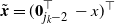$\tilde{{\textbf{\textit{x}}}}=({\textbf{0}}_{j_k-2}^\top\,-x)^\top$ . Furthermore, for $k=2,3,\ldots$ we have that, for all $x\geq 0$ ,

\begin{equation*} \text{P}(Y_k\leq x, T(i)=i, i=1,\ldots,k)=\Phi_{k-1}({\textbf{0}};\,\tilde{{\boldsymbol{\Omega}}})-\Phi_{k-1}(\tilde{{\textbf{\textit{x}}}};\,\tilde{{\boldsymbol{\Omega}}}), \end{equation*}

where $\tilde{{\textbf{\textit{x}}}}=({\textbf{0}}_{k-2}^\top\,-x)^\top$ , $\tilde{{\boldsymbol{\Omega}}}={\textbf{\textit{D}}}\bar{{\boldsymbol{\Sigma}}}_{\mathcal{I},\mathcal{I}}{\textbf{\textit{D}}}^\top$ , $\mathcal{I}=\{1,\ldots,k\}$ , $\mathcal{I}^{\text{c}}=\emptyset$ and ${\textbf{\textit{D}}}$ is as in Lemma 4.1.

Proof. By the total probability rule we have

\begin{align*} &\text{P}(X_{T(k)}-X_{T(k-1)}\leq x) \\ &\quad= \sum_{j_2=2}^\infty\sum_{j_3=j_2+1}^{\infty}\dots\sum_{j_k=j_{k-1}+1}^{\infty}\text{P}(X_{j_k}-X_{j_{k-1}}\leq x, T(i)=j_i,i=2,\dots,k). \end{align*}

Note that by repeating the same arguments as in the proof of Lemma 4.1 we obtain

\begin{equation*} \begin{split} &\text{P}(X_{j_k}-X_{j_{k-1}}\leq x, T(i)=j_i,i=2,\dots,k)\\ &=\text{P}(X_{j_k}-X_{j_{k-1}}\leq x, M_{j_{i-1}+1:j_{i}-1} <X_{j_{i-1}},X_{j_{i-1}}<X_{j_i},i=2,\dots,k)\\ &=\int_{-\infty}^{+\infty}\!\!\int_{z_k-x}^{z_k}\!\int_{-\infty}^{z_{k-1}}\!\!\!\!\!\!\dots\!\int_{-\infty}^{z_2}\text{P}(M_{j_{i-1}+1:j_{i}-1}<z_{i-1},i=2,\dots,k \mid X_{j_{l}}=z_{l},l=1,\dots,k)\\ &\qquad\qquad\qquad\qquad\qquad\cdot \phi_k(z_1,\dots,z_k)\,\mbox{d} z_1\dots\mbox{d} z_k\\ &=\int_{-\infty}^{+\infty}\int_{-\infty}^{z_{k}}\dots\int_{-\infty}^{z_2} \Phi_{j_k-k}({\boldsymbol{\varrho}}_{\mathcal{I}^{\text{c}},\mathcal{I}^{\text{c}}} {\boldsymbol{z}};\,\bar{{\boldsymbol{\Sigma}}}_{\mathcal{I}^{\text{c}},\mathcal{I}^{\text{c}};\mathcal{I}})\phi_k({\boldsymbol{z}};\,\bar{{\boldsymbol{\Sigma}}}_{\mathcal{I},\mathcal{I}})\,\mbox{d} {\boldsymbol{z}} \\ &\quad - \int_{-\infty}^{+\infty}\int_{-\infty}^{z_{k}-x}\dots\int_{-\infty}^{z_2} \Phi_{j_k-k}({\boldsymbol{\varrho}}_{\mathcal{I}^{\text{c}},\mathcal{I}^{\text{c}}} {\boldsymbol{z}};\,\bar{{\boldsymbol{\Sigma}}}_{\mathcal{I}^{\text{c}},\mathcal{I}^{\text{c}};\mathcal{I}})\phi_k({\boldsymbol{z}};\,\bar{{\boldsymbol{\Sigma}}}_{\mathcal{I},\mathcal{I}})\,\mbox{d} {\boldsymbol{z}}\\ &=\Phi_{j_k-k}({\textbf{0}};\,{\boldsymbol{\Gamma}}_{\mathcal{I}^{\text{c}}, \mathcal{I}^{\text{c}}})\text{P}(Z_1<Z_2<\dots<Z_k) \\ & \quad -\Phi_{j_k-k}({\textbf{0}};\,{\boldsymbol{\Gamma}}_{\mathcal{I}^{\text{c}}, \mathcal{I}^{\text{c}}})\text{P}(Z_1<Z_2<\dots<Z_k-x), \end{split} \end{equation*}

where ${\boldsymbol{\varrho}}_{\mathcal{I}^{\text{c}},\mathcal{I}^{\text{c}}}$ is given in (8) and ${\boldsymbol{\Gamma}}_{\mathcal{I}^{\text{c}}, \mathcal{I}^{\text{c}}}$ is given in (10). Once more, repeating the same reasoning as in the proof of Lemma 4.1, the result follows. Concluding, $\text{P}(Y_k\leq x, T(i)=i, i=1,\ldots,k)=\text{P}(X_k-X_{k-1},\leq x, X_1<X_2<\cdots<X_k)$ and therefore the result follows using similar steps to those in Lemma 4.1, but with $\mathcal{I}=\{1,\ldots,k\}$ , $\mathcal{I}^{\text{c}}=\emptyset$ .

Example 4.2. In the special case that $k=2$ in Proposition 4.1, the increment between the second and the third record is equal to

\begin{equation*} \text{P}(Y_2\leq x)= \sum_{n\geq 2} (\Phi_{n-1}({\textbf{0}};\,\tilde{{\boldsymbol{\Omega}}})-\Phi_{n-1}(\tilde{{\textbf{\textit{x}}}};\,\tilde{{\boldsymbol{\Omega}}})), \end{equation*}

where $\tilde{{\boldsymbol{\Omega}}}$ is as in (11). Furthermore, when $n=2$ we obtain ${\textbf{\textit{D}}}=(1\quad -1)$ , $\tilde{{\boldsymbol{\Omega}}}=2(1-\rho_1)$ , and therefore

(12) \begin{equation} \text{P}(Y_2\leq x)=1/2- \Phi({-}x/(2(1-\rho_1))^{1/2}). \end{equation}

5. Number of records

Let $N\,:\!=\sum_{n=1}^\infty {R}_{n}$ be the number of records among an infinite sequence $X_1,X_2,\ldots$ When the components of the sequence are independent and identically distributed with a continuous distribution function then it is a well-known result that an infinite number of records will occur: $E(N)=\sum_{n=1}^\infty P(R_n=1) = \sum_{n=1}^\infty 1/n =\infty$ [Reference Galambos11].

A natural question that arises is the following: What is the expected number of records that will take place in the case of a stationary Gaussian process?

Proposition 5.1. Let $\{X_n, n\geq 1\}$ be an SSG sequence of RVs and $\Phi_{n-1}({\textbf{0}};\,{\boldsymbol{\Gamma}}_{1:n-1;1:n-1})$ be the $\text{P}({R}_n=1)$ as described in Proposition 3.1. Let N be the number of records among an infinite sequence $X_1,X_2,\ldots$ Then we have

\begin{equation*} \text{E}(N)= \begin{cases} \infty, & \text{if} \quad 1/2\leq \gamma_{i,j;n}\leq 1, \quad \text{for all } 1\leq i\neq j < n , \\[5pt] 2, & \text{if} \quad \gamma_{i,j;n}=0 , \quad\;\;\; \qquad \text{for all } 1\leq i\neq j < n, \end{cases} \end{equation*}

where $\gamma_{i,j;n}$ is the correlation parameter in (4).

Proof. First, note that

\begin{equation*} \begin{split} \text{E}(N)&=\text{E}\bigg(\sum_{n=1}^\infty {R}_n\bigg)=\sum_{n=1}^\infty \text{E}({R}_n)\\ &=1+\sum_{n=2}^\infty \text{P}(X_{n}>M_{n-1})\\ &=1+\sum_{n=2}^\infty \Phi_{n-1}({\textbf{0}};\,{\boldsymbol{\Gamma}}_{1:n-1,1:n-1}). \end{split} \end{equation*}

The entries of the correlation matrix $\bar{{\boldsymbol{\Gamma}}}_{1:n-1,1:n-1}$ in (4) are $\gamma_{i,j;n}=1/2$ , $1\leq i\neq j<n$ , if and only if $\rho_{{\left\vert{\kern1.5ptj-i}\right\vert}}=\rho_{n-i}=\rho_{n-j}=0$ . In this case, by Remark 3.1 we have that $\Phi_{n-1}({\textbf{0}};\,{\textbf{\textit{I}}}_{n-1}+{\textbf{1}}_{n-1}{\textbf{1}}_{n-1}^\top)=1/n$ . From this it follows that when $1/2\leq \gamma_{i,j;n}\leq 1$ or

(13) \begin{equation} \sqrt{(1-\rho_{n-i})(1-\rho_{n-j})}\leq 1+\rho_{{\left\vert{\kern1.5ptj-i}\right\vert}} -\rho_{n-i}-\rho_{n-j} \leq 2\sqrt{(1-\rho_{n-i})(1-\rho_{n-j})}, \end{equation}

then $\Phi_{n-1}({\textbf{0}};\,{\boldsymbol{\Gamma}}_{1:n-1,1:n-1})\geq1/n$ , and as a consequence

\begin{equation*} \text{E}(N)\geq\sum_{n=1}^{\infty}\frac{1}{n}=\infty. \end{equation*}

For every $1\leq i\neq j < n$ , provided that $\rho_{n-i}+\rho_{n-j}\geq 0$ , when $\rho_{{\left\vert{\kern1.5ptj-i}\right\vert}}=\rho_{n-i}+\rho_{n-j}-1$ then we have $\bar{{\boldsymbol{\Gamma}}}_{1:n-1,1:n-1}={\textbf{\textit{I}}}_{n-1}$ . Therefore in this case $\Phi_{n-1}({\textbf{0}};\,{\boldsymbol{\Gamma}}_{1:n-1,1:n-1})=\Phi_{n-1}({\textbf{\textit{I}}}_{n-1})=2^{-n+1}$ . As a consequence,

() \begin{equation} \text{E}(N)=1+\sum_{n=2}^\infty2^{-n+1}=2\sum_{n=0}^\infty 2^{-n}-2 = 2. \end{equation}

From Proposition 5.1 it follows that the expected number of records depends on the type of correlation structure of the Gaussian process. For example, an infinite number of records is expected when all variables are uncorrelated, or when $X_i$ and $X_j$ are more correlated than the sum of the correlations between $X_i$ and $X_n$ , and $X_j$ and $X_n$ , for every $1\leq i\neq j < n$ . The second assertion follows from the left-hand side of the inequality in (13) by noting that $0\leq\sqrt{(1-\rho_{n-i})(1-\rho_{n-j})}\leq1$ . This suggests looking at $1+\rho_{{\left\vert{\kern1.5ptj-i}\right\vert}} -\rho_{n-i}-\rho_{n-j}\geq 1$ , which holds as soon as $\rho_{{\left\vert{\kern1.5ptj-i}\right\vert}}\geq\rho_{n-i}+\rho_{n-j}$ . Instead, loosely speaking, when $X_i$ and $X_j$ are less correlated than the sum of the correlations between $X_i$ and $X_n$ , and $X_j$ and $X_n$ , for every $1\leq i\neq j < n$ , the expected number of records can be finite. This assertion follows from the condition $\rho_{{\left\vert{\kern1.5ptj-i}\right\vert}}=\rho_{n-i}+\rho_{n-j}-1$ , provided that $\rho_{n-i}+\rho_{n-j}\geq 0$ , which leads to two records that should be expected. Finally, we remark that the case when $0<\gamma_{i,j;n}<1/2$ is still an open problem.

6. Joint records

In the case that $X_1,X_2,\ldots$ is a sequence of independent and exponential distributed RVs, the joint distribution of several numbers of consecutive records is well known in the literature (see, e.g., [Reference Galambos11]). For a general continuous distribution the asymptotic properties of consecutive joint records have been studied in [Reference Barakat and Elgawad6], and for non-consecutive joint records in [Reference Falk, Khorrami Chokami and Padoan10].

In this section, for a stationary time-dependent Gaussian process we study the probability that two records occur at prescribed indices, together with the distribution of such records. We start with the simpler case, i.e. two non-consecutive records. Then we study the case of two consecutive records.

The next theorem provides some results on two non-consecutive joint records.

Theorem 6.1. Let $\{X_n, n\geq 1\}$ be an SSG sequence of RVs. For every $n\geq 2$ and $j<n,$ let $\mathcal{I}=\{j,n\}$ and $\mathcal{I}^{\text{c}}=\{1,\ldots,j-1,j+1,\ldots,n-1\}$ . When $j=1,$ the probability that $X_j$ and $X_n$ are records, and the corresponding joint distribution, coincide with those given in Proposition 3.1. When $n\geq 3$ and $1<j<n,$ the probability that $X_j$ and $X_n$ are records is

(14) \begin{equation} \text{P}({R}_j=1, {R}_n=1)=\Phi_{n-1}({\textbf{0}};\, \tilde{{\boldsymbol{\Omega}}}), \end{equation}

where $\tilde{{\boldsymbol{\Omega}}}$ is given in (17). The joint distribution of $(X_j,X_n)$ , given that they are records, is

(15) \begin{equation} \text{P}(X_j\leq x_1, X_n\leq x_2\mid {R}_j=1, {R}_n=1)= \begin{cases} P(x_1,x_2), & x_1\leq x_2 , \\[4pt] P(x_2,x_2), & x_1> x_2 , \end{cases} \end{equation}

where

\begin{equation*} \begin{split} P(a,b)&= \frac{\Phi_{n-2}({\textbf{0}};\,{\boldsymbol{\Gamma}}_{{\mathcal{I}^{\text{c}}},{\mathcal{I}^{\text{c}}}})}{\Phi_{n-1}({\textbf{0}};\, \tilde{{\boldsymbol{\Omega}}})} \big(\Psi_{2,n-2}(a,b;\, \bar{{\boldsymbol{\Sigma}}}_{\mathcal{I},\mathcal{I}},{\boldsymbol{\varrho}}_{{\mathcal{I}^{\text{c}}}, {{\mathcal{I}^{\text{c}}}}},\bar{{\boldsymbol{\Sigma}}}_{{{\mathcal{I}^{\text{c}}}},{{\mathcal{I}^{\text{c}}}};\mathcal{I}})\\[4pt] &\quad-\Psi_{2,n-2}(a,a;\, \bar{{\boldsymbol{\Sigma}}}_{\mathcal{I},\mathcal{I}},{\boldsymbol{\varrho}}_{{\mathcal{I}^{\text{c}}}, {{\mathcal{I}^{\text{c}}}}},\bar{{\boldsymbol{\Sigma}}}_{{{\mathcal{I}^{\text{c}}}},{{\mathcal{I}^{\text{c}}}};\mathcal{I}})\\[4pt] &\quad+\Psi_{2,n-2}(0,a;\,{\textbf{\textit{D}}}\bar{{\boldsymbol{\Sigma}}}_{{\mathcal{I}},{\mathcal{I}}}{\textbf{\textit{D}}}^\top, {\boldsymbol{\Delta}},\bar{{\boldsymbol{\Sigma}}}^{**}_{{{\mathcal{I}^{\text{c}}}},{{\mathcal{I}^{\text{c}}}};\mathcal{I}})\big). \end{split} \end{equation*}

Proof. When $j=1$ we have $\text{P}({R}_1=1, {R}_n=1)=\text{P}({R}_n=1)$ , since $R_1=1$ is the certain event. Therefore, we only need to study the probability of a record at time n and the corresponding distribution. These are given in Proposition 3.1. When $n\geq 3$ and $1<j<n$ , with similar steps to those used in the proof of Proposition 3.1 we have that the probability that $X_j$ and $X_n$ are records is

\begin{equation*} \begin{split} \text{P}({R}_j&=1, {R}_n=1)=\text{P}(X_j>M_{j-1}, X_n>M_{n-1})\\ &=\int_{-\infty}^{+\infty}\int_{-\infty}^{z_2}\text{P}\left( M_{j-1}<z_1, M_{{j+1}:{n-1}}<z_2 \mid X_j=z_1, X_n=z_2\right)\phi_2(z_1,z_2;\,\bar{{\boldsymbol{\Sigma}}}_{\mathcal{I},\mathcal{I}})\,\mbox{d} z_1\,\mbox{d} z_2\\ &=\int_{-\infty}^{+\infty}\int_{-\infty}^{z_2}\Phi_{n-2}\left({\boldsymbol{\varrho}}_{{\mathcal{I}^{\text{c}}}, {{\mathcal{I}^{\text{c}}}}}{\boldsymbol{z}};\,\bar{{\boldsymbol{\Sigma}}}_{{{\mathcal{I}^{\text{c}}}},{{\mathcal{I}^{\text{c}}}};\,\mathcal{I}}\right)\phi_2({\boldsymbol{z}};\,\bar{{\boldsymbol{\Sigma}}}_{\mathcal{I},\mathcal{I}})\,\mbox{d} z_1\,\mbox{d} z_2\\ &=\Phi_{n-2}({\textbf{0}}, {\boldsymbol{\Gamma}}_{{\mathcal{I}^{\text{c}}},{\mathcal{I}^{\text{c}}}})\int_{-\infty}^{+\infty}\int_{-\infty}^{z_2}\psi_{2,n-2}\left({\boldsymbol{z}};\,\bar{{\boldsymbol{\Sigma}}}_{\mathcal{I},\mathcal{I}},{\boldsymbol{\varrho}}_{{\mathcal{I}^{\text{c}}}, {{\mathcal{I}^{\text{c}}}}},\bar{{\boldsymbol{\Sigma}}}_{{{\mathcal{I}^{\text{c}}}},{{\mathcal{I}^{\text{c}}}};\,\mathcal{I}}\right)\,\mbox{d} z_1\,\mbox{d} z_2\\ &=\Phi_{n-2}({\textbf{0}};\,{\boldsymbol{\Gamma}}_{{\mathcal{I}^{\text{c}}},{\mathcal{I}^{\text{c}}}})\text{P}(Z_1-Z_2<0), \end{split} \end{equation*}

where $(Z_1,Z_2)\sim \text{CSN}_{2,n-2}(\bar{{\boldsymbol{\Sigma}}}_{\mathcal{I},\mathcal{I}},{\boldsymbol{\varrho}}_{{\mathcal{I}^{\text{c}}}, {{\mathcal{I}^{\text{c}}}}},\bar{{\boldsymbol{\Sigma}}}_{{{\mathcal{I}^{\text{c}}}},{{\mathcal{I}^{\text{c}}}};\mathcal{I}})$ . Precisely, to obtain the third line we used the formula in (3) with

(16) \begin{align} \notag{\textbf{\textit{B}}}&= \begin{pmatrix} {\textbf{1}}_{j-1} & \quad {\textbf{0}}_{j-1}\\ {\textbf{0}}_{n-j-1} & \quad {\textbf{1}}_{n-j-1} \end{pmatrix},\\ \notag{\boldsymbol{\varrho}}_{{\mathcal{I}^{\text{c}}}, {{\mathcal{I}^{\text{c}}}}}&={\boldsymbol{\sigma}}_{{{\mathcal{I}^{\text{c}}}},{{\mathcal{I}^{\text{c}}}};\mathcal{I}}^{-1}({\textbf{\textit{B}}}-{\boldsymbol{\Sigma}}_{{{\mathcal{I}^{\text{c}}}}, {\mathcal{I}}}\bar{{\boldsymbol{\Sigma}}}_{{\mathcal{I}}, {\mathcal{I}}}^{-1}),\\ &= \begin{pmatrix} \frac{1}{\sigma_{11}}\left(1-\frac{\rho_{j-1}-\rho_{n-1}\rho_{n-j}}{1-\rho_{n-j}^2}\right) & \frac{\rho_{j-1}\rho_{n-j}-\rho_{n-1}}{\sigma_{11}(1-\rho_{n-j}^2)}\\ \vdots & \vdots\\ \frac{1}{\sigma_{j-1\,j-1}}\left(1-\frac{\rho_{1}-\rho_{n-j+1}\rho_{n-j}}{1-\rho_{n-j}^2}\right) & \frac{\rho_{1}\rho_{n-j}-\rho_{n-j+1}}{\sigma_{j-1\,j-1}(1-\rho_{n-j}^2)}\\ \frac{\rho_{n-j-1}\rho_{n-j}-\rho_{1}}{\sigma_{n-1\,n-1}(1-\rho_{n-j}^2)} & \frac{1}{\sigma_{n-1\,n-1}}\left(1-\frac{\rho_{n-j-1}-\rho_{1}\rho_{n-j}}{1-\rho_{n-j}^2}\right)\\ \vdots & \vdots\\ \frac{\rho_{1}\rho_{n-j}-\rho_{n-j-1}}{\sigma_{j+1\,j+1}(1-\rho_{n-j}^2)} & \frac{1}{\sigma_{j+1\,j+1}}\left(1-\frac{\rho_{1}-\rho_{n-j-1}\rho_{n-j}}{1-\rho_{n-j}^2}\right) \end{pmatrix}, \end{align}

$\bar{{\boldsymbol{\Sigma}}}_{{{\mathcal{I}^{\text{c}}}},{{\mathcal{I}^{\text{c}}}};\mathcal{I}}$ is an $(n-2)\times(n-2)$ partial correlation matrix with upper diagonal entries

\begin{equation*} \rho_{i,k;j,n}=\rho_{{\left\vert{\kern1.5ptj-i}\right\vert}}-\frac{\rho_{{\left\vert{\kern1.5ptj-i}\right\vert}}-\rho_{n-i}\rho_{n-j}}{1-\rho_{n-j}^2}\rho_{{\left\vert{\kern1.5ptj-k}\right\vert}}-\frac{\rho_{n-i}-\rho_{{\left\vert{\kern1.5ptj-i}\right\vert}}\rho_{n-j}}{1-\rho_{n-j}^2}\rho_{n-k}, \text{ for all } i<k\in {\mathcal{I}^{\text{c}}}, \end{equation*}

and

\begin{equation*} \begin{split} \sigma_{ii}&=1-\frac{\rho_{{\left\vert{\kern1.5ptj-i}\right\vert}}-\rho_{n-i}\rho_{n-j}}{1-\rho_{n-j}^2}\rho_{{\left\vert{\kern1.5ptj-i}\right\vert}}-\frac{\rho_{n-i}-\rho_{{\left\vert{\kern1.5ptj-i}\right\vert}}\rho_{n-j}}{1-\rho_{n-j}^2}\rho_{n-i}\\ &=1-\frac{\rho^2_{n-i}-\rho^2_{{\left\vert{\kern1.5ptj-i}\right\vert}}}{1-\rho_{n-j}^2}. \end{split} \end{equation*}

In the third line we multiply and divide the term within the integrals by $\Phi_{n-2}({\textbf{0}};\,{\boldsymbol{\Gamma}}_{{\mathcal{I}^{\text{c}}}, {{\mathcal{I}^{\text{c}}}}})$ , where ${\boldsymbol{\Gamma}}_{{\mathcal{I}^{\text{c}}}, {{\mathcal{I}^{\text{c}}}}}$ is defined as

\begin{equation*} {\boldsymbol{\Gamma}}_{{\mathcal{I}^{\text{c}}}, {{\mathcal{I}^{\text{c}}}}}={\boldsymbol{\varrho}}_{{\mathcal{I}^{\text{c}}}, {{\mathcal{I}^{\text{c}}}}}\bar{{\boldsymbol{\Sigma}}}_{\mathcal{I},\mathcal{I}}{\boldsymbol{\varrho}}_{{\mathcal{I}^{\text{c}}}, {{\mathcal{I}^{\text{c}}}}}^\top+\bar{{\boldsymbol{\Sigma}}}_{{{\mathcal{I}^{\text{c}}}},{{\mathcal{I}^{\text{c}}}};\mathcal{I}}. \end{equation*}

We therefore recognise a unified multivariate skew-normal PDF within the integrals, and its integral can be seen as $\text{P}(Z_1<Z_2)$ . Now, by (2) we obtain

\begin{equation*} Z_1-Z_2= \begin{pmatrix} 1 & -1 \end{pmatrix} \begin{pmatrix} Z_1\\ Z_2 \end{pmatrix} \sim \text{CSN}_{1,n-2}\left(2(1-\rho_{n-j}),{\boldsymbol{\Delta}}^*,{\boldsymbol{\Sigma}}^*_{{\mathcal{I}^{\text{c}}}, {{\mathcal{I}^{\text{c}}}};\mathcal{I}}\right) , \end{equation*}

where

\begin{equation*} \begin{split} {\boldsymbol{\Delta}}^*&=\frac{1}{2(1-\rho_{n-j})}{\boldsymbol{\varrho}}_{{\mathcal{I}^{\text{c}}}, {{\mathcal{I}^{\text{c}}}}}\bar{{\boldsymbol{\Sigma}}}_{\mathcal{I},\mathcal{I}} \begin{pmatrix} 1 \\ -1 \end{pmatrix}\\ &=\frac{1}{2}\begin{pmatrix} \left(\frac{1}{\sigma_{ii}}\left(1+\frac{\rho_{n-i}-\rho_{{\left\vert{\kern1.5ptj-i}\right\vert}}}{1-\rho_{n-j}}\right)\right)_{i=1,\dots,j-1}\, \left(\frac{1}{\sigma_{n+j-i\,n+j-i}}\left(\frac{\rho_{n-i}-\rho_{{\left\vert{i-j}\right\vert}}}{1-\rho_{n-j}}-1\right)\right)_{i=j+1,\dots,n-1} \end{pmatrix}^\top \end{split} \end{equation*}

and

\begin{equation*} {\boldsymbol{\Sigma}}^*_{{\mathcal{I}^{\text{c}}}, {{\mathcal{I}^{\text{c}}}};\mathcal{I}}={\boldsymbol{\Gamma}}_{{\mathcal{I}^{\text{c}}}, {{\mathcal{I}^{\text{c}}}}}-{\boldsymbol{\Delta}}^* \begin{pmatrix} 1-\rho_{n-j} & -1+\rho_{n-j} \end{pmatrix} {\boldsymbol{\varrho}}_{{\mathcal{I}^{\text{c}}}, {{\mathcal{I}^{\text{c}}}}}^\top. \end{equation*}

Using (1) we obtain the result, with

(17) \begin{equation} \tilde{{\boldsymbol{\Omega}}}= \begin{pmatrix} {\boldsymbol{\Gamma}}_{{\mathcal{I}^{\text{c}}}, {{\mathcal{I}^{\text{c}}}}} & -2(1-\rho_{n-j}){{\boldsymbol{\Delta}}^*}\\[5pt] -2(1-\rho_{n-j}){{\boldsymbol{\Delta}}^*}^\top & 2(1-\rho_{n-j}) \end{pmatrix}. \end{equation}

By similar steps we can compute the joint distribution of two records $(X_j,X_n)$ for $j<n$ :

\begin{align*} &\text{P}(X_j\leq x_1, X_n \leq x_2 \mid {R}_j=1, {R}_n=1) = \\ &\qquad\qquad\qquad\qquad\quad \frac{\text{P}(X_j\leq x_1, X_n\leq x_2, X_j>M_{j-1}, X_n>M_{n-1})}{\text{P}(X_j>M_{j-1}, X_n>M_{n-1})}. \end{align*}

The numerator can be written as

\begin{equation*} \begin{split} &\text{P}(X_j\leq x_1, X_n\leq x_2,X_j>M_{j-1}, X_n>M_{n-1})\\ &=\int_{-\infty}^{x_2}\int_{-\infty}^{\min(x_1,z_2)}\!\!\!\!\text{P}\left( M_{j-1}<z_1, M_{{j+1}:{n-1}}<z_2 \mid X_j=z_1, X_n=z_2\right)\phi({\boldsymbol{z}};\,\bar{{\boldsymbol{\Sigma}}}_{{\mathcal{I}},\mathcal{I}})\,\mbox{d} z_1\,\mbox{d} z_2\\ &=\int_{-\infty}^{x_2}\int_{-\infty}^{x_1}\text{P}\left( M_{j-1}<z_1, M_{{j+1}:{n-1}}<z_2 \mid X_j=z_1, X_n=z_2\right) \\ &\qquad\qquad\quad \cdot \phi_2({\boldsymbol{z}};\,\bar{{\boldsymbol{\Sigma}}}_{{\mathcal{I}},\mathcal{I}}){\mathbbm{1}}(z_2>x_1)\,\mbox{d} z_1\,\mbox{d} z_2\\ &+\int_{-\infty}^{x_2}\int_{-\infty}^{z_2}\text{P}\left( M_{j-1}<z_1, M_{{j+1}:{n-1}}<z_2 \mid X_j=z_1, X_n=z_2\right) \\ & \qquad\qquad\quad\cdot\phi_2({\boldsymbol{z}};\,\bar{{\boldsymbol{\Sigma}}}_{{\mathcal{I}},\mathcal{I}}){\mathbbm{1}}(z_2<x_1)\,\mbox{d} z_1\,\mbox{d} z_2\\ &=\int_{x_1}^{x_2}\int_{-\infty}^{x_1}\text{P}\left( M_{j-1}<z_1, M_{{j+1}:{n-1}}<z_2 \mid X_j=z_1, X_n=z_2\right)\phi_2({\boldsymbol{z}};\,\bar{{\boldsymbol{\Sigma}}}_{{\mathcal{I}},\mathcal{I}})\,\mbox{d} z_1\,\mbox{d} z_2\\ &+\int_{-\infty}^{x_1}\int_{-\infty}^{z_2}\text{P}\left( M_{j-1}<z_1, M_{{j+1}:{n-1}}<z_2 \mid X_j=z_1, X_n=z_2\right)\phi_2({\boldsymbol{z}};\,\bar{{\boldsymbol{\Sigma}}}_{{\mathcal{I}},\mathcal{I}})\,\mbox{d} z_1\,\mbox{d} z_2\\ &=\int_{-\infty}^{x_2}\int_{-\infty}^{x_1}\Phi_{n-2}\left({\boldsymbol{\varrho}}_{{\mathcal{I}^{\text{c}}}, {{\mathcal{I}^{\text{c}}}}}{\boldsymbol{z}};\,\bar{{\boldsymbol{\Sigma}}}_{{{\mathcal{I}^{\text{c}}}},{{\mathcal{I}^{\text{c}}}};\mathcal{I}}\right)\phi_2({\boldsymbol{z}};\,\bar{{\boldsymbol{\Sigma}}}_{{\mathcal{I}},\mathcal{I}})\,\mbox{d} z_1\,\mbox{d} z_2\\ &-\int_{-\infty}^{x_1}\int_{-\infty}^{x_1}\Phi_{n-2}\left({\boldsymbol{\varrho}}_{{\mathcal{I}^{\text{c}}}, {{\mathcal{I}^{\text{c}}}}}{\boldsymbol{z}};\,\bar{{\boldsymbol{\Sigma}}}_{{{\mathcal{I}^{\text{c}}}},{{\mathcal{I}^{\text{c}}}};\mathcal{I}}\right)\phi_2({\boldsymbol{z}};\,\bar{{\boldsymbol{\Sigma}}}_{{\mathcal{I}},\mathcal{I}})\,\mbox{d} z_1\,\mbox{d} z_2\\ &+\int_{-\infty}^{x_1}\int_{-\infty}^{z_2}\Phi_{n-2}\left({\boldsymbol{\varrho}}_{{\mathcal{I}^{\text{c}}}, {{\mathcal{I}^{\text{c}}}}}{\boldsymbol{z}};\,\bar{{\boldsymbol{\Sigma}}}_{{{\mathcal{I}^{\text{c}}}},{{\mathcal{I}^{\text{c}}}};\mathcal{I}}\right)\phi_2({\boldsymbol{z}};\,\bar{{\boldsymbol{\Sigma}}}_{{\mathcal{I}},\mathcal{I}})\,\mbox{d} z_1\,\mbox{d} z_2, \end{split} \end{equation*}

where ${\boldsymbol{\varrho}}_{{\mathcal{I}^{\text{c}}}, {{\mathcal{I}^{\text{c}}}}}$ is as in (16). We multiply and divide each term within the integrals by $\Phi_{n-2}({\textbf{0}};\,{\boldsymbol{\Gamma}}_{{\mathcal{I}^{\text{c}}}, {{\mathcal{I}^{\text{c}}}}})$ . Then, we recognise that the first two integrals provide the distribution of the CSN random vector we introduced before, evaluated at the points $(x_1,x_2)$ , $(x_1,x_1)$ . Instead, the third integral represents the distribution of the random vector $(Z_1-Z_2, Z_1)$ , which, again according to (2), follows a CSN distribution, i.e.

\begin{equation*} \begin{split} & \begin{pmatrix} 1\ \ & -1\\ 0\ \ &1 \end{pmatrix} \begin{pmatrix} Z_1\\ Z_2 \end{pmatrix} ={\textbf{\textit{D}}}\begin{pmatrix} Z_1\\ Z_2 \end{pmatrix} \sim \text{CSN}_{2,n-2}({\textbf{\textit{D}}}\bar{{\boldsymbol{\Sigma}}}_{{\mathcal{I}},{\mathcal{I}}}{\textbf{\textit{D}}}^\top,{\boldsymbol{\Delta}},\bar{{\boldsymbol{\Sigma}}}^{**}_{{{\mathcal{I}^{\text{c}}}},{{\mathcal{I}^{\text{c}}}};\mathcal{I}}), \end{split} \end{equation*}

where ${\boldsymbol{\Delta}}={\boldsymbol{\varrho}}_{{\mathcal{I}^{\text{c}}}, {{\mathcal{I}^{\text{c}}}}}\bar{{\boldsymbol{\Sigma}}}_{{{\mathcal{I}^{\text{c}}}},{{\mathcal{I}^{\text{c}}}}}{\textbf{\textit{D}}}^\top{({\textbf{\textit{D}}}\bar{{\boldsymbol{\Sigma}}}_{{\mathcal{I}},{\mathcal{I}}}{\textbf{\textit{D}}}^\top)}^{-1}$ , $\bar{{\boldsymbol{\Sigma}}}^{**}_{{{\mathcal{I}^{\text{c}}}},{{\mathcal{I}^{\text{c}}}};\mathcal{I}}={\boldsymbol{\Gamma}}_{{\mathcal{I}^{\text{c}}}, {{\mathcal{I}^{\text{c}}}}}-{\boldsymbol{\Delta}}{\textbf{\textit{D}}}\bar{{\boldsymbol{\Sigma}}}_{{\mathcal{I}},{\mathcal{I}}}{\boldsymbol{\varrho}}_{{\mathcal{I}^{\text{c}}},{\mathcal{I}^{\text{c}}}}^\top$ .

It follows from Theorem 6.1 that the two events of a record occurring at times j and n are not independent. Indeed, the probability $\Phi_{n-1}({\textbf{0}};\, \tilde{{\boldsymbol{\Omega}}})$ is different from the product of the two marginal probabilities $\Phi_{j-1}({\textbf{0}};\,{\boldsymbol{\Gamma}}_{1:j-1;1:j-1})$ and $\Phi_{n-1}({\textbf{0}};\,{\boldsymbol{\Gamma}}_{1:n-1;1:n-1})$ , derived in Proposition 3.1.

Remark 6.1. The marginal distribution of $X_j$ , given that $(X_j,X_n)$ are records, is

\begin{align*} \text{P}(X_j\leq x_1\mid {R}_j&=1, {R}_n=1)\\[4pt] &=\frac{\Phi_{n-2}({\textbf{0}};\,{\boldsymbol{\Gamma}}_{{\mathcal{I}^{\text{c}}},{\mathcal{I}^{\text{c}}}})}{\Phi_{n-1}({\textbf{0}};\, \tilde{{\boldsymbol{\Omega}}})} \times\big(\Psi_{1,n-2}(x_1;\, 1,{\boldsymbol{\Delta}}_1,\bar{{\boldsymbol{\Omega}}}_{{{\mathcal{I}^{\text{c}}}},{{\mathcal{I}^{\text{c}}}};\mathcal{I}}) \\[4pt] &\qquad\qquad\quad\shoveright{-\Psi_{2,n-2}(x_1,x_1;\, \bar{{\boldsymbol{\Sigma}}}_{\mathcal{I},\mathcal{I}},{\boldsymbol{\varrho}}_{{\mathcal{I}^{\text{c}}}, {{\mathcal{I}^{\text{c}}}}},\bar{{\boldsymbol{\Sigma}}}_{{{\mathcal{I}^{\text{c}}}},{{\mathcal{I}^{\text{c}}}};\mathcal{I}})\quad\ }\\[4pt] & \qquad\qquad\quad+\Psi_{2,n-2}(0,x_1;\,{\textbf{\textit{D}}}\bar{{\boldsymbol{\Sigma}}}_{{\mathcal{I}},{\mathcal{I}}}{\textbf{\textit{D}}}^\top, {\boldsymbol{\Delta}},\bar{{\boldsymbol{\Sigma}}}^{**}_{{{\mathcal{I}^{\text{c}}}},{{\mathcal{I}^{\text{c}}}};\mathcal{I}})\big), \end{align*}

where

\begin{align*} {\boldsymbol{\Delta}}_1 & = \begin{pmatrix} {\sigma_{ii}^{-1}(1-\rho_{{\left\vert{\kern1.5ptj-i}\right\vert}})}_{i=1,\dots,j-1}\; {\sigma_{n+j-i\,n+j-i}^{-1}(\rho_{n-i}-\rho_{{\left\vert{i-j}\right\vert}})}_{i=j+1,\dots,n-1} \end{pmatrix}^\top, \\ \bar{{\boldsymbol{\Omega}}}_{{{\mathcal{I}^{\text{c}}}},{{\mathcal{I}^{\text{c}}}};\mathcal{I}}&=\bar{{\boldsymbol{\Sigma}}}_{{{\mathcal{I}^{\text{c}}}},{{\mathcal{I}^{\text{c}}}};\mathcal{I}}+{\boldsymbol{\Delta}}_1 {\textbf{\textit{A}}} \,\bar{{\boldsymbol{\Sigma}}}_{\mathcal{I},\mathcal{I}}{\boldsymbol{\varrho}}_{{\mathcal{I}^{\text{c}}}, {{\mathcal{I}^{\text{c}}}}}\\ &=\bar{{\boldsymbol{\Sigma}}}_{{{\mathcal{I}^{\text{c}}}},{{\mathcal{I}^{\text{c}}}};\mathcal{I}}- {\boldsymbol{\Delta}}_1 {\boldsymbol{\Delta}}_1^\top, \end{align*}

and these parameters are obtained from (2) with ${\textbf{\textit{A}}}\,:\!=(1\quad 0)$ . See the proof of Theorem 6.1 for details. Hence, similarly to the case of independent random variables in [Reference Falk, Khorrami Chokami and Padoan10], the distribution of $X_j$ being a record is affected by the additional knowledge that $X_n$ is a record, if we know that $X_n$ is a record as well. The marginal distribution of $X_n$ , given that $(X_j,X_n)$ are records, is

\begin{equation*} \text{P}(X_n\leq x_2\mid {R}_j=1, {R}_n=1)= \frac{\Phi_{n-2}({\textbf{0}};\,{\boldsymbol{\Gamma}}_{{\mathcal{I}^{\text{c}}},{\mathcal{I}^{\text{c}}}})}{\Phi_{n-1}({\textbf{0}};\, \tilde{{\boldsymbol{\Omega}}})} \Psi_{2,n-2}(0,x_2;\,{\textbf{\textit{D}}}\bar{{\boldsymbol{\Sigma}}}_{{\mathcal{I}},{\mathcal{I}}}{\textbf{\textit{D}}}^\top, {\boldsymbol{\Delta}},\bar{{\boldsymbol{\Sigma}}}^{**}_{{{\mathcal{I}^{\text{c}}}},{{\mathcal{I}^{\text{c}}}};\mathcal{I}}). \end{equation*}

Hence, different to the case of independent random variables in [Reference Falk, Khorrami Chokami and Padoan10], we have that the distribution of $X_n$ , being a record, is affected by the additional knowledge that at time $j<n$ there was a record.

In the next result we add the assumption that the two records in Theorem 6.1 are consecutive.

Proof. First, we compute the probability that two consecutive records occur. For every $1\leq\, j<n$ we have

\begin{equation*} \begin{split} &\text{P}({R}_j=1, {R}_n=1,S)=\text{P}(X_i<X_j, \text{ for all } i\in{\mathcal{I}^{\text{c}}}, X_n>X_j)\\ &=\int_{-\infty}^{+\infty}\int_{-\infty}^{z_2}\text{P}\left( X_i<z_1, \text{ for all } i\in{\mathcal{I}^{\text{c}}} \mid X_j=z_1, X_n=z_2\right)\phi_2(z_1,z_2;\bar{{\boldsymbol{\Sigma}}}_{\mathcal{I},\mathcal{I}})\,\mbox{d} z_1\,\mbox{d} z_2\\ &=\int_{-\infty}^{+\infty}\int_{-\infty}^{z_2}\Phi_{n-2}\left({\boldsymbol{\varrho}}_{{\mathcal{I}^{\text{c}}}, {{\mathcal{I}^{\text{c}}}}}{\boldsymbol{z}};\,\bar{{\boldsymbol{\Sigma}}}_{{{\mathcal{I}^{\text{c}}}},{{\mathcal{I}^{\text{c}}}};\mathcal{I}}\right)\phi_2({\boldsymbol{z}};\,\bar{{\boldsymbol{\Sigma}}}_{\mathcal{I},\mathcal{I}})\,\mbox{d} z_1\,\mbox{d} z_2, \end{split} \end{equation*}

where the last line is obtained from (3) with

\begin{align*} \notag{\textbf{\textit{B}}}&= \begin{pmatrix} {\textbf{1}}_{n-2}\ \ & {\textbf{0}}_{n-2} \end{pmatrix},\\ \notag{\boldsymbol{\varrho}}_{{\mathcal{I}^{\text{c}}}, {{\mathcal{I}^{\text{c}}}}}&={\boldsymbol{\sigma}}_{{{\mathcal{I}^{\text{c}}}},{{\mathcal{I}^{\text{c}}}};\mathcal{I}}^{-1}({\textbf{\textit{B}}}-{\boldsymbol{\Sigma}}_{{{\mathcal{I}^{\text{c}}}}, {\mathcal{I}}}\bar{{\boldsymbol{\Sigma}}}_{{\mathcal{I}}, {\mathcal{I}}}^{-1})\\ &= \begin{pmatrix} \frac{1}{\sigma_{11}}\Big(1-\frac{\rho_{j-1}-\rho_{n-1}\rho_{n-j}}{1-\rho_{n-j}^2}\Big) & \frac{\rho_{j-1}\rho_{n-j}-\rho_{n-1}}{\sigma_{11}(1-\rho_{n-j}^2)}\\ \vdots & \vdots\\ \frac{1}{\sigma_{j-1\,j-1}}\Big(1-\frac{\rho_{1}-\rho_{n-j+1}\rho_{n-j}}{1-\rho_{n-j}^2}\Big) & \frac{\rho_{1}\rho_{n-j}-\rho_{n-j+1}}{\sigma_{j-1\,j-1}(1-\rho_{n-j}^2)}\\[12pt] \frac{1}{\sigma_{j+1\,j+1}}\Big(1-\frac{\rho_{1}-\rho_{n-j-1}\rho_{n-j}}{1-\rho_{n-j}^2}\Big) & \frac{\rho_{1}\rho_{n-j}-\rho_{n-j-1}}{\sigma_{j+1\,j+1}(1-\rho_{n-j}^2)}\\[12pt] \frac{1}{\sigma_{j+2\,j+2}}\Big(1-\frac{\rho_{2}-\rho_{n-j-2}\rho_{n-j}}{1-\rho_{n-j}^2}\Big) & \frac{\rho_{2}\rho_{n-j}-\rho_{n-j-2}}{\sigma_{j+2\,j+2}(1-\rho_{n-j}^2)}\\ \vdots & \vdots\\ \frac{1}{\sigma_{n-1\,n-1}}\Big(1-\frac{\rho_{n-j-1}-\rho_{1}\rho_{n-j}}{1-\rho_{n-j}^2}\Big) & \frac{\rho_{1}\rho_{n-j}-\rho_{n-j-1}}{\sigma_{n-1\,n-1}(1-\rho_{n-j}^2)} \end{pmatrix}. \end{align*}

The remaining part of this proof is the same as the proof of Theorem 6.1.

The joint distribution of $(X_j,X_n)$ is given by

\begin{align*} &\text{P}\left(X_j\leq x_1, X_n \leq x_2 \mid {R}_j=1, {R}_n=1,S\right) \\ &\quad= \frac{\text{P}\left(X_j\leq x_1, X_n\leq x_2, X_i<X_j, \text{ for all } i\in{\mathcal{I}^{\text{c}}}, X_n>X_j\right)}{\text{P}(X_i<X_j, \text{ for all } i\in{\mathcal{I}^{\text{c}}}, X_n>X_j)}. \end{align*}

Note that

\begin{align*} &\text{P}(X_j\leq x_1, X_n\leq x_2, X_i<X_j, \text{ for all } i\in{\mathcal{I}^{\text{c}}}, X_n>X_j)\\ &\quad=\int_{-\infty}^{x_2}\int_{-\infty}^{\min(x_1,z_2)}\text{P}\left(X_i<z_1, \text{ for all } i\in{\mathcal{I}^{\text{c}}} \mid X_j=z_1, X_n=z_2\right)\phi({\boldsymbol{z}};\,\bar{{\boldsymbol{\Sigma}}}_{{\mathcal{I}},\mathcal{I}})\,\mbox{d} z_1\,\mbox{d} z_2. \end{align*}

Therefore, the remaining part of the proof is the same as the proof of Theorem 6.1. Thus the proof is complete.

Appendix A. Complementary results

As an alternative to the discussion in Section 4, we discuss here another approach for deriving the distribution for the arrival time of the second record and the distribution of the increment $Y_2\,:\!=X_{T(2)}-X_1$ . This method benefits from simpler notation, but it seems harder to extend to higher-order records.

Proposition A.1. Let $\{X_n, n\geq 1\}$ be an SSG sequence of RVs with autocorrelation $0\leq \rho_{{\left\vert{\kern1.5ptj-i}\right\vert}}< 1$ for $1\leq i$ , $j\leq n$ . For $n=2,3,\ldots$ , the distribution of the arrival time of the second record T(2) is

(18) \begin{equation} \text{P}\left(T(2)=n\right)= \begin{cases} 1/2, & n=2,\\ \Phi_{n-2}({\textbf{0}};\,{\boldsymbol{\Gamma}}_{2:n-1,2:n-1})- \Phi_{n-1}({\textbf{0}};\,{\boldsymbol{\Gamma}}_{2:n,2:n}), & n> 2, \end{cases} \end{equation}

where ${\boldsymbol{\Gamma}}_{2:n-1,2:n-1}$ and ${\boldsymbol{\Gamma}}_{2:n,2:n}$ are defined similarly to (5). Furthermore, for every $x>0$ , the distribution of the increment $Y_2\,:\!=X_{T(2)}-X_1$ is

(19) \begin{equation} \text{P}(Y_2\leq x)=\sum_{n\geq 2} \Phi_{n-1}\left({\textbf{\textit{u}}}_x;{\boldsymbol{\Gamma}}_{2:n,2:n}\right)-\Phi_{n-1}\left({\textbf{0}};\,{\boldsymbol{\Gamma}}_{2:n,2:n}\right), \end{equation}

where ${\textbf{\textit{u}}}_x=(x/(1-\rho^2_{n-1})^{1/2},0,\ldots,0)^\top$ is an $(n-1)$ -dimensional vector. When $n=2$ we have $u_x=x/(1-\rho_{1}^2)^{1/2}$ .

Proof. When $n=2$ we have

\begin{equation*} \text{P}(T(2)=2)=\text{P}(X_2>X_1)=1/2. \end{equation*}

For $n>2$ we have

\begin{equation*} \begin{split} \text{P}(T(2)=n)&=\text{P}\left( X_i<X_1,\,i=2,\dots,n-1,X_n>X_1\right)\\ &=\text{P}\left( X_i<X_1,\,i=2,\dots,n-1\right)-\text{P}\left( X_i<X_1,\,i=2,\dots,n\right). \end{split} \end{equation*}

Therefore, (18) follows by similar arguments to those used in Proposition 3.1.

Finally, for every $x>0$ the distribution of the increment $Y_2$ is

\begin{equation*} \begin{split} \text{P}(Y_2\leq x)&=\sum_{n\geq 2}\text{P}(X_n-X_1\leq x,T(2)=n)\\ &=\sum_{n\geq 2}\text{P}(X_n-X_1\leq x,X_i<X_1,\,i=2,\dots,n-1,X_n>X_1)\\ &=\sum_{n\geq 2}\text{P}(0<X_n-X_1\leq x,X_i<X_1,\,i=2,\dots,n-1). \end{split} \end{equation*}

The term inside the sum is equal to

\begin{equation*} \begin{split} &\text{P}(0<X_n-X_1\leq x,X_i<X_1,\,i=2,\dots,n-1)\\ &=\int_{-\infty}^{+\infty}\text{P}(0<X_n-z\leq x,X_i<z,\,i=2,\dots,n-1\mid X_1=z)\phi(z)\,\mbox{d} z\\ &=\int_{-\infty}^{+\infty}\text{P}(X_i<z,\,i=2,\dots,n-1,X_n\leq z+x\mid X_1=z)\phi(z)\,\mbox{d} z\\ &\quad-\int_{-\infty}^{+\infty}\text{P}(X_i<z,\,i=2,\dots,n\mid X_1=z)\phi(z)\,\mbox{d} z. \end{split} \end{equation*}

Therefore, (19) follows by similar arguments to those used in Proposition 3.1.

Remark A.1. Note that when $\rho_{{\left\vert{\kern1.5ptj-i}\right\vert}}=0$ for all $1\leq i$ , $j\leq n$ and $n>2$ we obtain, by exploiting the result in Remark 3.1,

\begin{align*} \text{P}\left(T(2)=n\right) & = \Phi_{n-2}({\textbf{0}};\,{\textbf{\textit{I}}}_{n-2}+{\textbf{1}}_{n-2}{\textbf{1}}_{n-2}^\top)- \Phi_{n-1}({\textbf{0}};\,{\textbf{\textit{I}}}_{n-1}+{\textbf{1}}_{n-1}{\textbf{1}}_{n-1}^\top) \\ & =\frac{1}{n-1}-\frac{1}{n}=\frac{1}{n(n-1)}, \end{align*}

as expected.

Remark A.2. Note also that when $n=2$ in (19) we obtain

\begin{equation*} \text{P}(Y_2\leq x)=\Phi(x/(2(1-\rho_1))^{1/2}) -1/2, \end{equation*}

which is consistent with the result in (12).

Ultimately, observe that for the result in (18) of Proposition A.1 it should be checked that

(20) \begin{align}\nonumber\sum_{n\geq 2} \text{P}(T(2)=n)&=\frac{1}{2}+\lim_{N\to\infty}\sum_{n=3}^N\left(\Phi_{n-2}({\textbf{0}};\,{\boldsymbol{\Gamma}}_{2:n-1,2:n-1})-\Phi_{n-1}({\textbf{0}};\,{\boldsymbol{\Gamma}}_{2:n,2:n})\right)\\\nonumber&=\lim_{N\to\infty}\left(1-\Phi_{2}\left({\textbf{0}};\,{\boldsymbol{\Gamma}}_{1:2,1:2}\right)+\Phi_{2}\left({\textbf{0}};\,{\boldsymbol{\Gamma}}_{1:2,1:2}\right)\right.\\\nonumber&\left.\quad-\dots+\Phi_{N-2}\left({\textbf{0}};\,{\boldsymbol{\Gamma}}_{1:N-2,1:N-2}\right)-\Phi_{N-1}\left({\textbf{0}};\,{\boldsymbol{\Gamma}}_{1:N-1,1:N-1}\right)\right)\\&=1-\lim_{N\to\infty}\Phi_{N-1}\left({\textbf{0}};\,{\boldsymbol{\Gamma}}_{1:N-1,1:N-1}\right)=1.\end{align}

To show that the limit in (20) converges to zero may not be easy without any restrictions on the correlation structure of the Gaussian sequence. We succeed in this task by assuming the following setup.

Consider a triangular array of Gaussian RVs $X_{n,i}$ with $i=1,2,\ldots$ and $n=1,2,\ldots$ (see, e.g., [Reference Hsing, Hüsler and Reiss16]). Assume that for each given n we have that $\{X_{n,i}, i\geq 1\}$ is an SSG sequence satisfying the condition $\rho_{n,{\left\vert{\kern1.5ptj-i}\right\vert}}\to 0$ as $|\kern1.5ptj-i|\to \infty$ , where $\rho_{n,{\left\vert{\kern1.5ptj-i}\right\vert}}=\text{E}(X_{n,i}X_{n,j})$ . At the same time, assume also that the correlations among neighbouring observations of $\{X_{n,i}, i\geq 1\}$ increase to 1 as the row number n increases, i.e. $\rho_{n,{\left\vert{\kern1.5ptj-i}\right\vert}}\to 1$ as $n\to\infty$ , for any $1<i$ , $j<\infty$ fixed. In the following we write $X_1,\ldots, X_n$ in place of $X_{n,1},\ldots, X_{n,n}$ for $n=1,2,\ldots$ , in order to simplify the notation.

We assume in Proposition A.1 that for each n, $X_1,\ldots,X_n$ is an SSG sequence corresponding to a triangular array of Gaussian RVs (as described above). In this setting we want to derive the limit in (20). Then, let $(\tilde{X}_1,\ldots,\tilde{X}_{n-1})$ be a zero-mean unit-variance Gaussian sequence with variance-covariance matrix ${\boldsymbol{\Gamma}}_{1:n-1,1:n-1}$ , and set $P_n=\text{P}(\tilde{X}_i\leq 0,\ldots,\tilde{X}_{n-1}\leq 0)=\Phi_{n-1}\left({\textbf{0}};\,{\boldsymbol{\Gamma}}_{1:n-1,1:n-1}\right)$ . Clearly, $\Phi_{n-1}\left({\textbf{0}};\,{\boldsymbol{\Gamma}}_{1:n-1,1:n-1}\right)=\Phi_{n-1}\left({\textbf{0}};\bar{{\boldsymbol{\Gamma}}}_{1:n-1,1:n-1}\right)$ . We recall that $\text{P}(\tilde{X}_i\leq0)=1/2$ for every $i=1,\ldots,n-1$ . By the Fréchet inequalities we have that

\begin{equation*}A_n\,:\!=\max\bigg(0,\sum_{i=1}^n\text{P}(X_i\leq0)-(n-1)\bigg)=\max(0,1-n/2)\leq P_n \leq 1/2.\end{equation*}

For $P_n$ we derive the following upper bound $B_n$ . Precisely,

\begin{align*} P_n&=\text{P}\bigg(\sum_{i=1}^{n-1}{\mathbbm{1}}(\tilde{X}_i\leq 0)\geq n-1\bigg)=\text{P}\bigg\{\sum_{i=1}^{n-1}\bigg({\mathbbm{1}}(\tilde{X}_i\leq 0)-\frac 12\bigg)\geq \frac{n-1}{2}\bigg\}\\ &\leq \text{P}\bigg\{\bigg|\sum_{i=1}^{n-1}\bigg({\mathbbm{1}}(\tilde{X}_i\leq 0)-\frac 12\bigg)\bigg|\geq \frac{n-1}{2}\bigg\}\\ &\leq \frac{4}{(n-2)^2}\text{E}\bigg[\bigg\{ \sum_{i=1}^{n-1}\bigg({\mathbbm{1}}(\tilde{X}_i\leq 0)-\frac 12\bigg) \bigg\}^2\bigg]\\ &= \frac{4}{(n-2)^2} \sum_{i=1}^{n-1} \sum_{j=1}^{n-1}\text{cov}({\mathbbm{1}}(\tilde{X}_i\leq 0), {\mathbbm{1}}(\tilde{X}_j\leq 0))\\ &= \frac{4}{(n-2)^2} \sum_{i=1}^{n-1} \sum_{j=1}^{n-1}(P_{i,j;n}-1/4)=\!:\, B_n, \end{align*}

where $P_{i,j;n}\,:\!=\text{P}(\tilde{X}_i\leq 0,\tilde{X}_j\leq 0)=\Phi_2(0;\gamma_{i,j;n})$ and where $\Phi_2(\cdot;\gamma_{i,j;n})$ is a bivariate Gaussian CDF with correlation $\gamma_{i,j;n}$ that is given in (4). In the third row we used Chebyshev’s inequality. Setting $h=|\kern1.5ptj-i|$ , we rewrite $B_n$ as

\begin{align*} \nonumber B_n & = \frac{4(n-1)}{(n-2)^2} (P_{0;n}-1/4) + \frac{8}{(n-2)^2}\sum_{h=1}^{n-2}\left(n-h-1\right)(P_{h;n}-1/4)\\ & = \alpha_n+\beta_n, \end{align*}

where $P_{h;n}\,:\!=\text{P}(\tilde{X}_0\leq 0,\tilde{X}_h\leq 0)=\Phi_2(0;\gamma_{i,j;n})$ , and we recall that

(21) \begin{equation}\gamma_{i,j;n}=\frac{1+\rho_{|\kern1.5ptj-i|} -\rho_{n-i}-\rho_{n-j}}{2\sqrt{(1-\rho_{n-i})(1-\rho_{n-j})}\,},\qquad |\kern1.5ptj-i|=0,\ldots,n-2.\end{equation}

Now, when $h=0$ we have $\rho_{|\kern1.5ptj-i|}=1$ and $\rho_{n-i}=\rho_{n-j}$ . Therefore, we obtain $\gamma_{i,j;n}=1$ and as a consequence $P_{0;n}=1/2$ . From this it follows that

\begin{equation*}\alpha_n=\frac{(n-1)}{(n-2)^2}\to 0, \qquad n\to\infty.\end{equation*}

We rewrite the term $\beta_n$ as

\begin{align*} \beta_n & = \frac{8}{n(1-2/n)^2}\sum_{h=1}^{n-2}(P_{h;n}-1/4)- \frac{8}{n(1-2/n)^2}\sum_{h=1}^{n-2}\frac{h}{n}(P_{h;n}-1/4)\\ & = c_n - d_n. \end{align*}

Now we consider the case $h\geq 1$ . Assuming the index i fixed, we rewrite $j=n-k$ with $1\leq k \leq n-j$ . The same reasoning can be repeated, interchanging the rules between i and j. From (21) we then have

(22) \begin{equation}\gamma_{i,j;n}\approx \frac{1+\rho_{|n-k-i|} -\rho_{k}}{2\sqrt{(1-\rho_{k})}}, \qquad n\to\infty.\end{equation}

When $|\kern1.5ptj-i|$ is small compared to n, i.e. $k=n-j$ with the index j fixed, then from (22) we obtain $\gamma_{i,j;n}\approx (1+\rho_{|\kern1.5ptj-i|})/2$ as $n\to\infty$ . In this case $1/2<\gamma_{i,j;n}<1$ . When $|\kern1.5ptj-i|$ approaches infinity, i.e. k is a small value compared to n, then from (22) we obtain $\gamma_{i,j;n}\approx \sqrt{1-\rho_{k}}/2$ as $n\to\infty$ . Since $\rho_k\to 1$ as $n\to \infty$ by the assumption stemming from the triangular array setting, we then have that $\gamma_{i,j;n}\to 0$ as $n\to \infty$ . Therefore, for all $\varepsilon>0$ there exists an $n_0$ such that for all $h>n_0$ we have $|P_{h;n}-1/4|<\varepsilon$ . As a consequence we have

\begin{align*} c_n & = \frac{8}{n(1-2/n)^2}\bigg(\sum_{h=1}^{n_0}(P_{h;n}-1/4)+\sum_{h=n_0+1}^{n-2}(P_{h;n}-1/4)\bigg)\\ & < \frac{8}{n(1-2/n)^2}\left(c + \varepsilon(n-2+n_0+1) \right)=o(1), \end{align*}

where c is a positive constant. Therefore, $c_n\to 0$ as $n\to \infty$ and since $d_n<c_n$ then $\beta_n\to 0$ and $B_n\to0$ as $n\to \infty$ . Concluding, since $A_n\leq P_n\leq B_n$ and $A_n=0$ for $n\geq 2$ , then $P_n\to0$ as $n\to\infty$ .