



1. Introduction
Power-law shot noise models are a key class of physical models for long-range dependence and self-similarity; see, e.g., [Reference Lowen and Teich31, Chapter 9] and [Reference Pipiras and Taqqu39, Section 3.4]. They frequently arise in applications such as wireless networks [Reference Van Der Ziel47], finance [Reference Klüppelberg and Kühn26, Reference Schmidt46], insurance [Reference Brémaud8, Reference Ganesh and Torrisi16, Reference Klüppelberg and Mikosch27], and queueing theory [Reference Boxma and Mandjes7, Reference Ganesh, O’Connell and Wischik15, Reference Pang and Zhou36, Reference Whitt50]. A shot noise process captures the cumulative effect of arriving noise (or ‘shots’) whose influence persists according to certain response functions. When the noise is independent and identically distributed with a finite second moment, the integrated shot noise process converges weakly to a fractional Brownian motion (FBM); see, e.g., [Reference Klüppelberg and Kühn26] and [Reference Pipiras and Taqqu39, Chapter 3.4]. When the noise has an infinite second moment, such as belonging to the domain of attraction of a symmetric
 $\alpha$
-stable distribution, the scaling limit of the integrated shot noise process may be a fractionally integrated
 $\alpha$
-stable Lévy process; see, e.g., [Reference Iksanov22, Chapter 3.3] and [Reference Klüppelberg, Mikosch and Schärf28].
Non-stationary shot noise processes are widely used to model many stochastic systems [Reference Armony, Israelit, Mandelbaum, Marmor, Tseytlin and Yom-Tov3, Reference Pang and Zhou36–Reference Pang and Zhou38]. Recently, [Reference Pang and Taqqu35] studied a class of integrated non-stationary shot noise processes where the noise is assumed to be conditionally independent given the arrival times, with the distribution of each noise depending on its arrival time. In [Reference Pang and Taqqu35, Theorem 3.1], it is shown that the scaled integrated shot noise process converges in distribution to a generalized FBM [Reference Chang, Yao and Zajic11]. This weak convergence result intuitively suggests that a sample path moderate deviation principle (MDP) for the scaled integrated shot noise process can be formulated, based on the limiting generalized FBM. The objective of this paper is to establish the MDP rigorously.
Large and moderate deviation principles for Poisson shot processes and related models have been extensively studied [Reference Boxma, Cahen, Koops and Mandjes6, Reference Budhiraja and Nyquist9–Reference Chang, Yao and Zajic11, Reference Duffield and O’Connell13, Reference Ganesh, Macci and Torrisi14, Reference Gao and Wang18, Reference Jiang and Yang23, Reference Kozachenko, Vasylyk and Sottinen29, Reference Majewski34, Reference Rhee, Blanchet and Zwart43, Reference Yan and Gao51]. However, most of these studies focus on situations where the increments are either independent or stationary. In those cases, Ottaviani’s inequality and the maximal inequalities for martingales [Reference Puhalskii41] play important roles in the proofs. When the noise is neither independent nor identically distributed, as in the framework of [Reference Pang and Taqqu35], no such maximal inequality is available, to the best of our knowledge. In this paper, we address this difficulty by applying Schied’s exponential tightness criterion on the path space [Reference Schied44, Reference Schied45] to replace the maximal inequality.
Recently, [Reference Anugu and Pang1, Theorem 3.1] established the large deviation principle (LDP) for the generalized Riemann–Liouville FBM – see (17) – by using the weak convergence approach. Building on this LDP result, the LDP for a stochastic fluid queue with a generalized Riemann–Liouville FBM as the input process was obtained in [Reference Anugu and Pang1, Theorem 4.1], the existence of a steady-state distribution was derived in [Reference Anugu and Pang1, Corollary 5.1], and the exact logarithmic tail asymptotics for the steady-state distribution were obtained in [Reference Anugu and Pang1, Theorem 5.4]. These results extend those of [Reference Chang, Yao and Zajic10] regarding the stochastic fluid queue with a Riemann–Liouville FBM as the input process.
As pointed out in [Reference Anugu and Pang2, Introduction], two asymptotic scaling regimes for shot noise processes have been studied in the literature. The first is the conventional time-space scaling regime, where time is sped up and space is scaled down. The second is known as the high-intensity regime, in which the arrival rate is scaled up while time remains unchanged in the shot response function, and space is scaled down. The sample path MDP for shot noise processes in the high-intensity regime was established in [Reference Anugu and Pang2, Theorem 2.1]. The approach was based on the Dawson–Gärtner theorem [Reference Dembo and Zeitouni12, Theorem 4.6.1], the Gärtner–Ellis theorem [Reference Dembo and Zeitouni12, Theorem 2.3.6], and exponential tightness in appropriate functional spaces. However, shot noise processes with non-Markovian and non-stationary characteristics, as considered in [Reference Anugu and Pang2], introduce new challenges. They applied a maximal inequality for the sum of independent random variables (which are not necessarily identically distributed), as well as Lusin’s theorem for exponential tightness. In comparison, they also established the sample-path MDP result in the conventional time–space scaling regime (see [Reference Anugu and Pang2, Theorem 2.2]). Although both scaling regimes yield MDPs with the same speed function, the rate functions differ significantly. For more details, see [Reference Anugu and Pang2, Remarks 2.8, 2.9].
The MDP result in this paper (see Theorem 2) also applies to the conventional time–space scaling regime. However, we remove [Reference Anugu and Pang2, Assumption 2.1 (A.4)] for the integrated shot noise process (3). This introduces difficulties in proving an MDP for finite-dimensional distributions (see Lemma 3) and exponential tightness (see Lemma 5). Surprisingly, by applying Schied’s exponential tightness criterion on the path space from [Reference Schied44, Reference Schied45] and utilizing Hölder’s continuity of the limiting process X (see (7)), we are able to prove Lemmas 3 and 5 using the same strategy. We believe this method will also be useful for studying the sample path MDP for shot noise processes in the high-intensity regime.
1.1. Organization of the paper
In Section 2, we first describe the model of non-stationary power-law shot noise processes and state the assumptions on the scaled processes. We then present a functional central limit theorem in the space of continuous functions, followed by the sample path MDP result for non-stationary power-law shot noise processes and its applications to fluid queues with integrated shot noise process input. The proofs of the central limit theorem and MDP are provided in Sections 3 and 4, respectively. The proofs for the associated fluid queues are given in Section 5. A proof of the MDP without the fourth-moment condition (Condition 5) is provided in Section 6. Finally, a short proof of Schied’s exponential tightness criterion [Reference Schied44] is included in the Appendix.
1.2. Notation
Throughout the paper, let
 $\mathbb{Z}$
and
 $\mathbb{N}$
denote the sets of integers and natural numbers respectively, and let
 $\mathbb Z_*=\mathbb Z\setminus\{0\}$
,
 $\mathbb N_*= \mathbb N\setminus\{0\}$
. We denote by
 $\mathcal{D}[0,T]$
the space of all càdlàg functions on the interval [0,T], equipped with the Skorokhod
 $J_1$
-norm. Similarly, we denote by
 $\mathcal{C}[0,T]$
the space of all continuous functions on [0,T], equipped with the uniform norm
 $\|z\|_T={\sup}_{t\in [0,T]}|z(t)|$
. For more details on these spaces and their properties, see, e.g., [Reference Billingsley4].
2. The models, main results, and applications
2.1. Non-stationary power-law shot noise processes
As in [Reference Pang and Taqqu35], we consider the shot noise process
 $S^*=\{S^*(y)\}_{y\in \mathbb R}$
defined by
 \begin{equation} S^*(y)\,:\!=\sum_{j\in \mathbb Z_*} g^*(y-S_j)R_j(S_j), \quad y\in \mathbb R,\end{equation}
where
 $\{S_j\}_{j\in \mathbb Z_*}$
is a sequence of Poisson arrival times with rate 1, satisfying
 $\cdots < S_{-1} < 0 < S_1 < \cdots$
, and
 $R_j$
denotes the noise caused by the shot at the time
 $S_j$
. The non-negative shot shape function
 $g^*$
accounts for the lingering effect of the noise shocks.
Assume that the random variables
 $\{R_j\}_{j\in \mathbb Z_*}$
are conditionally independent given
 $\{S_j\}_{j\in \mathbb Z_*}$
, and that, for each
 $j \in \mathbb Z_*$
, the distribution of
 $R_j$
depends on the time
 $S_j$
. Specifically, for any
 $u,r \in \mathbb R$
, we have the conditional distribution
 $\mathbb P(R_j\le r\mid S_j=u)=F_u(r)$
. We write
 $R_j(S_j)$
to indicate explicitly that
 $R_j$
depends on
 $S_j$
.
Condition 1.
Given the arrival times
 $\{S_j\}_{j\in \mathbb Z_*}$
, we assume that the conditional mean of
 $R_j$
is zero, and the conditional variance of
 $R_j$
is finite. Specifically, for each
 $u \in \mathbb R\setminus\{0\}$
,
 \begin{equation} K_1(u)\,:\!=\int_{\mathbb R}r\,{\mathrm{d}} F_u(r)=0, \qquad K_2(u)\,:\!=\int_{\mathbb R}r^2\,{\mathrm{d}} F_u(r)\in(0,\infty). \end{equation}
Furthermore, we assume that
 $K_2(u)=|u|^{-\gamma}\tilde L(u)\mathbf{1}_{\{u\neq0\}}$
, where
 $\gamma\in(0,1)$
is a constant,
 $\tilde L(u)$
is a positive slowly varying function at
 $\pm\infty$
, and
 $\tilde L(u)$
is bounded away from 0 and
 $\infty$
on every compact subset of
 $\mathbb R$
.
Consider the integrated shot noise process
 $S\,:\!=\{S(t)\}_{t\in \mathbb R_+}$
defined by
 \begin{equation} S(t)\,:\!=\sum_{j\in \mathbb Z_*}\big(g(t-S_j)-g(\!-S_j)\big) R_j(S_j), \quad t\in \mathbb R_+,\end{equation}
where
 $S(0)=0$
, and the shot shape function g(t) is given by
 \begin{equation} g(t)\,:\!=\int_0^t g^*(y)\,{\mathrm{d}} y, \quad t\in \mathbb R_+.\end{equation}
We assume that the function
 $g^*$
satisfies the following condition.
Condition 2.
There exists a constant
 $\beta\in\big(\frac12-{\gamma}/{2}, 1\big)$
such that
 \begin{equation} g^*(y)\,:\!=y^{-\beta}L^*(y) \mathbf{1}_{\{y>0\}}, \end{equation}
where
 $L^*$
is a positive slowly varying function at
 $+\infty$
that is bounded away from 0 and
 $\infty$
on every bounded subset of
 $[0,\infty)$
.
Under Condition 2, by using [Reference Bingham, Goldie and Teugels5, Proposition 1.5.8] we know that the function g in (4) satisfies
 $g(t)=t^{1-\beta}L(t)\mathbf{1}_{\{t\ge0\}}$
, where L is a positive slowly varying function bounded away from 0 and
 $\infty$
on every bounded subset of
 $[0,\infty)$
, and
 $L(t) \sim {L^*(t)}/({1-\beta})$
as
 $t\rightarrow\infty$
. Let N be a Poisson random measure on
 $(\mathbb R^2, \mathcal B(\mathbb R^2))$
with intensity
 ${\mathrm{d}} F_u(r)\,{\mathrm{d}} u$
, that is,
-
(i) N is independently scattered on
 $(\mathbb R^2, \mathcal B(\mathbb R^2))$
, i.e. for any disjoint sets
$G_1,\ldots,G_n$
,
$N(G_1),\ldots,N(G_n)$
are independent;
-
(ii) for any bounded Borel set
$G \in \mathcal B(\mathbb R^2)$
, N(G) is a Poisson random variable with mean
$\int_{G}{\mathrm{d}} F_u(r)\,{\mathrm{d}} u$
.





Let
 $\widetilde N$
be the compensated Poisson measure defined by
 $\widetilde N(G)=N(G)-\int_G {\mathrm{d}} F_u(r)\,{\mathrm{d}} u$
for any bounded Borel set
 $G \in \mathcal B(\mathbb R^2)$
. Since the conditional mean of
 $R_j$
in (2) is zero, the integrated shot noise process
 $\{S(t)\}_{t\in \mathbb R_+}$
can be written as
 \begin{equation*} S(t) = \int_{-\infty}^t\int_{-\infty}^{\infty}\big(g(t-u)-g(\!-u)\big)r\widetilde N({\mathrm{d}} u,{\mathrm{d}} r), \quad t\ge 0.\end{equation*}
The integral on the right-hand-side is well defined in the sense of [Reference Rajput and Rosinski42], since
 \begin{align} \mathbb E[S(t)^2] & = \int_{-\infty}^t\int_{-\infty}^{\infty}\big(g(t-u)-g(\!-u)\big)^2 r^2\,{\mathrm{d}} F_u(r)\,{\mathrm{d}} u \nonumber \\ & = \int_{-\infty}^t\big(g(t-u)-g(\!-u)\big)^2 K_2(u)\,{\mathrm{d}} u, \end{align}
which is finite under Conditions 1 and 2. We also refer to [Reference Pipiras and Taqqu39, Appendix B.1.4] for more information on integration with respect to Poisson measures.
2.2. Weak convergence of the scaled integrated shot noise process
Condition 3.
Let
 $b\colon\mathbb N_*\rightarrow\mathbb R_+$
be a function that satisfies
 \begin{equation*} \lim_{n\rightarrow\infty}\frac{b(n)}{n^{{3}/{2}-\beta-{\gamma}/{2}}L(n)\tilde L(n)^{1/2}} = 1. \end{equation*}
When
 $\beta\in\big(\frac12,1\big)$
and
 $\gamma\in(0,1)$
, under Conditions 1–3 and the fourth moment condition of the distribution
 $F_u$
(see (9)), [Reference Pang and Taqqu35, Theorem 3.1 and Remark 3.3] proved that, as
 $ n\rightarrow\infty$
,
 $\{{S(nt)}/{b(n)}\}_{t\in [0,T]}$
converges weakly to a generalized fractional Brownian motion (GFBM) X in
 $(\mathcal D[0,T], J_1)$
, where
 $X\,:\!=\{X(t)\}_{t\in [0,T]}$
is defined by the integral representation
 \begin{equation*} X(t) =\int_{\mathbb R}\big((t-u)_+^{1-\beta}-(\!-u)_+^{1-\beta} \big)|u|^{-{\gamma}/{2}}\,B({\mathrm{d}} u),\end{equation*}
with
 $u_+ = \max\{0, u\}$
for all
 $u \in \mathbb R$
, and
 $B({\mathrm{d}} u)$
a Gaussian random measure on
 $\mathbb R$
with the Lebesgue control measure
 ${\mathrm{d}} u$
. The process X is a continuous mean-zero Gaussian process with
 $X(0)=0$
, and it has the self-similarity property with Hurst parameter
 $H=\frac32-\beta-{\gamma}/{2}$
. When
 $\gamma=0$
, X becomes a standard FBM with Hurst parameter H; when
 $\gamma\in (0,1)$
, X is a GFBM as defined in [Reference Pang and Taqqu35]. A GFBM preserves the self-similarity property, while the factor
 $|u|^{-{\gamma}/{2}}$
introduces the non-stationarity of increments, making it suitable for modeling non-stationary physical systems. For example, [Reference Ichiba, Pang and Taqqu21] studied the semimartingale properties of GFBMs, and applied them to model volatility processes in finance.
It follows from [Reference Ichiba, Pang and Taqqu20, Theorem 3.1] that for any
 $\gamma\in(0,1)$
,
 $\beta\in\big(\frac12-{\gamma}/{2},1\big)$
, there exists a constant
 $c_{2,1}(\gamma, \beta)\in (0,\infty)$
such that, for any
 $t, s\ge0$
,
 \begin{equation} \mathbb E[|X(t)-X(s)|^2] = \int_{\mathbb R}\big((t-u)_+^{1-\beta}-(s-u)_+^{1-\beta}\big)^2|u|^{-\gamma}{\mathrm{d}} u \le c_{2,1}(\gamma,\beta)|t-s|^{3-2\beta-\gamma}.\end{equation}
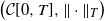
The following theorem proves the convergence of
 $\{S(nt)/b(n)\colon t\in[0,T]\}_{n\in\mathbb N_*}$
in the space
 $\big(\mathcal C[0,T], \|\cdot\|_T\big)$
.
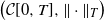
Theorem 1. Assume that Conditions 1–3 hold with
 $\gamma\in(0,1)$
and
 $\beta\in\big(\frac12-{\gamma}/{2},1-{\gamma}/{2}\big)$
. Then, as
 $ n\rightarrow\infty$
,
 $\{S(nt)/ b(n)\}_{t\in [0,T]}$
converges weakly to GFBM X in
 $\big(\mathcal C[0,T], \|\cdot\|_T\big)$
.
Remark 1. Compared with [Reference Pang and Taqqu35, Theorem 3.1], Theorem 1 does not assume the fourth moment condition on
 $F_u$
, and the convergence of the processes occurs in the function space
 $\big(\mathcal C[0,T]$
,
 $\|\cdot\|_{T}\big)$
, replacing the Skorokhod space
 $(\mathcal D[0,T], J_1)$
used in [Reference Pang and Taqqu35]. If
 $\gamma=0$
, then the range of
 $\beta$
in Theorem 1 is
 $\big(\frac12,1\big)$
, which coincides with the result for the standard FBM (see, e.g., [Reference Pipiras and Taqqu39, Theorem 3.3.8]).
2.3. Sample path MDP
To establish the sample path MDP for the integrated shot noise processes with Poisson arrivals and non-stationary noise, we impose the following conditions.
Condition 4.
There are constants
 $u_0>0$
and
 $\theta_0>0$
such that
 $K_2(u)=|u|^{-\gamma}\tilde L(u)\mathbf{1}_{\{|u|\ge u_0\}}$
, where
 $\tilde L(u)$
is a positive slowly varying function at
 $\pm\infty$
that it is bounded away from 0 and
 $\infty$
on every compact subset of
 $\mathbb R$
, and
 \begin{equation} M_{\theta_0} \,:\!= {\sup}_{u\in\mathbb R}\int_{\mathbb R}\exp\!\big(\theta_0|r|\big)\,{\mathrm{d}} F_u(r) < +\infty. \end{equation}
Condition 5.
There exists a positive constant
 $\kappa < \infty$
such that, for all
 $|u|\ge u_0$
,
 \begin{equation} \frac{K_4(u)}{K_2(u)^2}\le \kappa, \end{equation}
where
 $K_4(u) = \int_{\mathbb R}r^4\,{\mathrm{d}} F_u(r)$
.
Example 1. Suppose that
 $F_u$
is Gaussian with mean zero and variance
 $K_2(u) = |u|^{-\gamma}\mathbf{1}_{\{|u|\ge u_0\}}$
for
 $\gamma \in (0,1)$
. Then Conditions 4 and 5 are satisfied.
Condition 6.
Assume that the function
 $\pi\colon\mathbb R_+\rightarrow\mathbb R_+$
satisfies the following conditions:
 \begin{equation*} \lim_{n\rightarrow\infty}\pi(n) = \infty, \qquad \lim_{n\rightarrow\infty}\frac{\pi(n)}{n^{1/2-{\gamma}/{2}}\tilde L(n)^{1/2}} = 0. \end{equation*}
For any
 $n>0$
and
 $t\ge0$
, we define
 \begin{equation} S_n(t)\,:\!= \frac{S(nt)}{b(n)\pi(n)}.\end{equation}
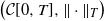
Theorem 2. Assume Conditions 1–6 hold with
 $\gamma\in(0,1)$
and
 $\beta\in\big(\frac12-{\gamma}/{2},1\big)$
. Then, as
 $n\rightarrow\infty$
,
 $\{S_n(t)\colon t\in[0,T]\}_{n\in \mathbb N_*}$
satisfies the large deviation principle on
 $\big(\mathcal C[0,T],\|\cdot\|_{T}\big)$
with the speed function
 $\pi(n)^2$
and the good rate function
 $I_{\beta,\gamma}$
given by
 \begin{equation} I_{\beta,\gamma}(\xi) \,:\!= \inf_{\mathcal S_{\xi}}\frac{1}{2} \int_{-\infty}^T\psi(u)^2\,{\mathrm{d}} u, \end{equation}
where, for
 $\xi\in\mathcal C[0,T]$
,
 $\mathcal S_{\xi}$
is the collection of all
 $\psi\in L^2((\!-\infty,T],\mathbb R)$
such that
 $$ \xi(t) = \int_{-\infty}^t\big((t-u)_+^{1-\beta}-(\!-u)_+^{1-\beta} \big)|u|^{-{\gamma}/{2}}\psi(u)\,{\mathrm{d}} u \quad \text{for } t\in [0,T]. $$
To explain why the distribution
 $F_u$
is assumed to be degenerate when u is in a neighborhood of the origin, let us recall that, when applying the Gärtner–Ellis theorem [Reference Dembo and Zeitouni12, Section 2.3], it is usually required that, for every
 $\theta$
in a neighborhood of the origin,
 \begin{equation} \Lambda(\theta) \,:\!= \lim_{n\rightarrow\infty}\frac{1}{\pi(n)^2}\log\mathbb E[\exp\!(\theta\pi(n)^2S_n(t))] \ \text{exists as a real number.}\end{equation}
For the MDP of the empirical mean of independent and identically distributed random variables, Condition (12) reduces to the well-known Cramér condition; see, e.g., [Reference Dembo and Zeitouni12, Theorem 3.7.1] or [Reference Gao17, Theorem 1].
Let us continue with Example 1. If
 $F_u$
is Gaussian with mean zero and variance
 $K_2(u) = |u|^{-\gamma}\mathbf{1}_{\{|u|\neq 0\}}$
for
 $\gamma \in (0,1)$
then, for every
 $\theta>0$
,
 $\mathbb E[\!\exp(\theta\pi(n)^2S_n(t))] = \infty$
, which contradicts (12). Thus, to study the MDP, it is necessary to assume that
 $F_u$
is degenerate when
 $|u|< u_0$
for some
 $u_0>0$
, which is equivalent to saying that there is no noise when the shot time
 $|S_j|<u_0$
for every
 $j\in \mathbb Z_*$
. Under this condition, the integrated shot noise process
 $\{S(t)\}_{t\in[0,T]}$
defined by (3) becomes the following truncated model:
 \begin{equation} \tilde S(t) \,:\!= \sum_{j\in\mathbb Z_*}\big(g(t-S_j)-g(\!-S_j)\big)R_j(S_j)\mathbf{1}_{\{|S_{j}|\ge u_0\}}, \quad t\in\mathbb R_+.\end{equation}
Since
 $S_j\rightarrow+\infty$
as
 $|j|\rightarrow\infty$
, the truncation can only affect a finite number of terms in (13). Therefore,
 $\{\tilde S(nt)/b(n)\}_{t\in [0,T]}$
shares many properties of
 $\{S(nt)/b(n)\}_{t\in [0,T]}$
. In particular, Theorem 1 also holds for
 $\{\tilde S(nt)/b(n)\colon t\in[0,T]\}_{n\in \mathbb N_*}$
under Conditions 1–3.
2.4. Applications
Shot noise processes and integrated shot noise processes have been applied to model the claim amount processes in insurance risk theory or input processes in queueing theory [Reference Brémaud8, Reference Ganesh and Torrisi16, Reference Klüppelberg and Mikosch27, Reference Klüppelberg, Mikosch and Schärf28, Reference Pang and Taqqu35, Reference Whitt50]. Those models are also applied to study the dynamics in storage systems or dams [Reference Prabhu40].
The process
 $\{S(t)\}_{t\ge0}$
in the context of insurance can be interpreted as follows. Consider an insurance company with initial capital
 $M_{0}>0$
, premium rate
 $\nu_{1}>0$
, and insurance rate
 $\nu_2\in(0,\nu_1)$
. Suppose that claims occur according to a renewal process
 $\{S_j\}_{j\in \mathbb Z_*}$
, and that the insurance company pays claims occurring at time
 $\{S_j\}_{j\in \mathbb Z_*}$
, at the rate
 $g^*(\!\cdot-S_j) R_j(S_j)+\nu_{2} $
, with
 $g^*(\!\cdot\!)$
given in (1). Then, the total claim paid in the time interval (0,t] is the integrated shot noise process
 $\{S(t)+\nu_2 t\}_{t\ge0}$
, with S(t) defined in (3). See [Reference Ganesh and Torrisi16] for further details.
Write
 $\nu=\nu_{1}-\nu_{2}$
. For any
 $t\ge0$
, let
 \begin{equation} M(t) \,:\!= {\sup}_{0\le s\le t}(S(s)-\nu s); \qquad V(t) \,:\!= {\sup}_{0\le s\le t}(S(t)-S(s)-\nu(t-s)). \end{equation}
Then,
 $M(t)>0$
represents the event of the insurance company’s ruin in the time interval [0,t], and V(t) is the total amount of residual claims, which are paid from the claims occurring up to time t. In the language of queueing models,
 $\{S(t)+\nu_2t\}_{t\ge0}$
is called an input process,
 $\{M(t)\}_{t\ge0}$
is called a running maximum process, and
 $\{V(t)\}_{t\ge0}$
is called a workload process [Reference Prabhu40, Reference Whitt50].
A systematic method for generating an input process that exhibits long-range dependence was developed in [Reference Chang, Yao and Zajic10, Reference Chang, Yao and Zajic11],] which showed that
 $V^{n}=\{V(nt)/t\colon t\ge0\}_{n\in\mathbb N_*}$
and
 $M^{n}=\{M(nt)/t\colon t\ge0\}_{n\in\mathbb N_*}$
satisfy the MDP [Reference Chang, Yao and Zajic10, Theorem 4.1, Lemma 5.2] and that the limit
 $M(\infty)$
has a sub-exponential tail distribution [Reference Chang, Yao and Zajic10, Theorem 5.1]. On the other hand, [Reference Anugu and Pang1] studied the LDP for the stochastic fluid queue with the generalized Riemann–Liouville FBM as the input process, examining the long-time behavior of the processes
 $\{M(t)\}_{t\ge0}$
and
 $\{V(t)\}_{t\ge0}$
, as defined by (14), with S replaced by the generalized Riemann–Liouville FBM. The methods there rely on large deviation theory and some special properties of the generalized Riemann-Liouville FBM.
We are interested in the asymptotic probabilities of the following events associated with the integrated shot noise process, as
 $t\rightarrow\infty$
:
-
(i) the ruin probability of the insurance company in the time interval [0, t], i.e.
$$ \mathbb P\big({\sup}_{0\le s\le t}(S(s) - \nu s) > M_{0}\big); $$
-
(ii) the probability that the total amount of residual claims paid from the time of the claim to time t exceeds a given value
$M_{1}$
, i.e.
$$ \mathbb P\big({\sup}_{0\le s\le t}(S(t)-S(s)-\nu(t-s)) > M_{1}\big). $$


Next, we give estimates for these probabilities using the MDP in Theorem 2. Let
 $c_{\beta,\gamma} = \int_{\mathbb R}\big((1-u)_+^{1-\beta}-(-u)_+^{1-\beta}\big)^2|u|^{-\gamma}\,{\mathrm{d}} u$
.
Proposition 1. Assume that Conditions 1–5 hold with
 $\gamma\in(0,1)$
and
 $\beta\in\big(\frac12-{\gamma}/{2},1-\gamma\big)$
.
-
(i) For all
$\lambda > 0$
, (15)where
\begin{equation} \lim_{n\rightarrow\infty}\frac{b(n)^2}{n^2}\log\mathbb P\bigg(\frac{M(n)}{n}>\lambda\bigg) = -\mathcal I(\lambda), \end{equation}
\begin{equation*} \mathcal I(\lambda) = \left\{ \begin{array}{l@{\quad}l} \dfrac{(\lambda+\nu)^2}{2c_{\beta,\gamma}} & if \ \lambda\ge\dfrac{\nu(1-H)}{H}, \\ \dfrac{\nu^{2H}}{2c_{\beta,\gamma}H^{2H}(1-H)^{2(1-H)}}\lambda^{2(1-H)} \quad & if\ \lambda < \dfrac{\nu(1-H)}{H}. \end{array} \right. \end{equation*}
-
(ii) For any
$\lambda >0$
, (16)where, for any
\begin{equation} \lim_{n\rightarrow\infty}\frac{b(n)^2}{n^2}\log\mathbb P(V(n)>\lambda) = -\inf_{0\le s\le 1}\frac{(\nu(1-s)+\lambda)^2}{v_1(s)+v_2(s)}, \end{equation}
$s\in (\!-\infty, 1]$
,
$v_1(s) = \int_{-\infty}^s\big[(1-u)^{1-\beta}-(s-u)^{1-\beta}\big]^2|u|^{-\gamma}\,{\mathrm{d}} u$
and
$v_2(s) = \int_s^1(1-u)^{2(1-\beta)}|u|^{-\gamma}\,{\mathrm{d}} u$
.




Proposition 2. Under the conditions of Proposition 1, M(t) converges almost surely to a finite random variable
 $M(\infty)$
, which has a sub-exponential tail distribution. Specifically,
 $$ \lim_{n\rightarrow\infty}\frac{b(n)^2}{n^2}\log\mathbb P(M(\infty)>n) = -\frac{\nu^{2H}}{2c_{\beta,\gamma}H^{2H}(1-H)^{2(1-H)}}. $$
Remark 2.
-
(i) In this subsection, to study the long-time behavior of the running maximum process M(n) and workload process V(n), we assume a stronger condition:
$\beta\in\big(\frac12-{\gamma}/{2}, 1-\gamma\big)$
, in which case the Hurst parameter of GFBM X is
$H=\frac{3}{2}-\beta-{\gamma}/{2} \in \big(\frac12,1\big)$
. This is the long-range dependence case. If
$H<\frac{1}{2}$
, the limiting behavior may be different. This condition is also necessary for the study of the long-term behaviors of these two processes for the stochastic fluid queue with input a (generalized Riemann–Louisville) FBM; see [Reference Chang, Yao and Zajic10, Theorem 3.1] and [Reference Anugu and Pang1, Remark 5.1]. -
(ii) In queueing theory, the steady-state limit
is obtained through the limit of
$$V(\infty)\,:\!=\lim_{t\rightarrow\infty}{\sup}_{0\le s\le t}(Y(t)-Y(s)-\nu (t-s))$$
$M(t)={\sup}_{0\le s\le t}(Y(s)-\nu s)$
. The key linkage between these two processes is the stationary increment property of the input process Y, which ensures that
$V(\infty)$
and
$M(\infty)$
are equal in distribution. If the input process Y has non-stationary increments, there is no simple way to ensure the existence of
$V(\infty)$
. By using the self-similarity and the modulus of continuity-type estimates of the input process Y, [Reference Anugu and Pang1, Corollary 5.1, Theorem 5.4] established that the law of V(t) has a weak limit as
$t\rightarrow\infty$
, and further derived the exact tail asymptotics for the steady state of V. See [Reference Anugu and Pang1, p. 64] for more details. However, those two approaches do not apply to the queueing process with the integrated shot noise process S(t) input (see (3)), since it lacks both properties of stationary increments and self-similarity.







2.5. The shot noise process with positive Poisson arrival times of shots
Consider the integrated shot noise process
 $\widetilde S\,:\!=\{\widetilde S(t)\}_{t\in \mathbb R_+}$
defined by
 \begin{equation*} \widetilde S(t) \,:\!= \sum_{j\in\mathbb N_*}\big(g(t-S_j)-g(\!-S_j)\big)R_j(S_j), \quad t\in \mathbb R_+.\end{equation*}
Here, the processes g,
 $\{S_j\}_{j\in \mathbb N_*}$
, and
 $\{R_j\}_{j\in \mathbb N_*}$
satisfy Conditions 1 and 2 with
 $\gamma\in(0,1)$
and
 $\beta\in\big(\frac12-{\gamma}/{2},1\big)$
.
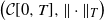
When b(n) satisfies Condition 3, by following similar steps to the proof of Theorem 1, we can show that
 $\{{\widetilde S(nt)}/{b(n)}\}_{t\in [0,T]}$
converges weakly to
 $\{Z(t)\}_{t\in[0,T]}$
in
 $\big(\mathcal C[0,T],\|\cdot\|_T\big)$
as
 $n\rightarrow \infty$
. Here,
 $\{Z(t)\}_{t \ge 0}$
is the generalized Riemann–Liouville FBM defined by
 \begin{equation} Z(t)\,:\!=\int_0^t(t-u)^{1-\beta}u^{-{\gamma}/{2}}B({\mathrm{d}} u), \quad t\ge0,\end{equation}
where
 $B({\mathrm{d}} u)$
is a Gaussian measure. This process was introduced in [Reference Pang and Taqqu35, Remark 5.1] and further studied in [Reference Ichiba, Pang and Taqqu20, Section 2.2] and [Reference Wang and Xiao49, Section 3].
For every
 $n\in\mathbb N_*$
and
 $t\in[0,T]$
, let
 $\widetilde S_n(t)$
be defined as in (10) with S(nt) replaced by
 $\widetilde S(nt)$
. By following the same reasoning as in the proof of Theorem 2 we obtain that, under the same conditions as Theorem 2,
 $\{\widetilde S_n(t)\colon t\in[0,T]\}_{n\in\mathbb N_*}$
satisfies the LDP on
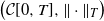 $\big(\mathcal C[0,T], \|\cdot\|_{T}\big)$
as
 $n\rightarrow\infty$
, with speed function
 $\pi(n)^2$
and good rate function
 $\widetilde I_{\beta,\gamma}$
given by
 \begin{equation} \widetilde I_{\beta,\gamma}(\xi) \,:\!= \inf_{\psi\in\widetilde{\mathcal S}_{\xi}}\frac{1}{2}\int^T_{0}\psi(u)^2\,{\mathrm{d}} u,\end{equation}
where, for
 $\xi\in\mathcal C[0,T]$
,
 $\widetilde{\mathcal S}_{\xi}$
is the collection of all
 $\psi\in L^2[0,T]$
such that
 $$\xi(t) = \int_{0}^t\big((t-u)_+^{1-\beta}-(\!-u)_+^{1-\beta}\big)|u|^{-{\gamma}/{2}}\psi(u)\,{\mathrm{d}} u \quad\text{for } t\in[0,T].$$
Notice that the rate function
 $\widetilde I_{\beta,\gamma}(\xi)$
in (18) is exactly the rate function for LDP of the generalized Riemann–Liouville FBM; see [Reference Anugu and Pang1, Theorem 3.1].
As an application of the LDP for
 $\{\widetilde S_n\}_{n\ge1}$
, following the steps in Section 2.4, we can also obtain similar results for
 $\widetilde M$
and
 $\widetilde V$
, where
 $\widetilde M(t) \,:\!= {\sup}_{0\le s\le t}(\widetilde S(s)-\nu s)$
and
 $\widetilde V(t) \,:\!= {\sup}_{0\le s\le t}(\widetilde S(t)-\widetilde S(s)-\nu(t-s))$
.
2.6. Results without Condition 5
When Condition 5 is absent, by using a strategy similar to the one in the previous subsections we can prove the same conclusion as Theorem 2, provided that the function
 $\pi(n)$
has a slower rate as n tends to infinity. More precisely, we assume
 $\pi(n)$
satisfies the following condition.
Condition 7.
Assume that there exists some constant
 $\eta>0$
satisfying
 $\lim_{n\rightarrow\infty} \pi(n)= \infty$
and
 \begin{equation*} \lim_{n\rightarrow\infty} \frac{\pi(n)}{n^{1/2-{\gamma}/{2}-\eta}}=0. \end{equation*}


3. Proof of Theorem 1
For any
 $n\in\mathbb N_*$
, let
 $\hat S_n(t)= {S(nt)}/{b(n)}$
for all
 $t\ge0$
.
3.1. Two lemmas
First, we provide a uniform moment estimate for the increments of
 $\hat S_n$
.
Lemma 1. Assume that Conditions 1–3 hold with
 $\gamma\in(0,1)$
and
 $\beta\in\big(\frac12-{\gamma}/{2}, 1-{\gamma}/{2}\big)$
. Then, for any
 $0 < \eta < \min\{2\beta+\gamma-1,2-2\beta-\gamma\}$
there exist positive constants
 $c_{3,1}$
and
 $c_{3,2}$
such that, for any
 $n>c_{3,2}$
,
 \begin{equation} \mathbb E\big[|\hat S_n(t)-\hat S_n(s)|^2\big] \le c_{3,1}|t-s|^{3-2\beta-\gamma-\eta} \quad \text{for all } s,t\in [0,T] . \end{equation}
Consequently, by Kolmogorov’s continuity theorem (see, e.g., [Reference Khoshnevisan24, Theorem C.6]),
 $\hat S_n$
has a modification, still denoted by
 $\hat S_n$
, that is almost surely continuous on [0, T].
Proof. For any
 $n>0$
,
 $0\le s < t\le T$
, we write
 \begin{align*} \hat S_n(t)-\hat S_n(s) & = \frac{1}{b(n)}\int_{-\infty}^{ns}\int_{-\infty}^{\infty}\big(g(nt-u)-g(ns-u)\big)r\,N({\mathrm{d}} u,{\mathrm{d}} r) \\ & \quad + \frac{1}{b(n)}\int_{ns}^{nt}\int_{-\infty}^{\infty}g(nt-u)r\,N({\mathrm{d}} u,{\mathrm{d}} r). \end{align*}
Since the two terms on the right-hand side are independent and have expectation zero, we have
 \begin{align} \mathbb E\big[(\hat S_n(t)-\hat S_n(s))^2\big] & = \frac{1}{b(n)^2}\int_{-\infty}^{ns}\big(g(nt-u)-g(ns-u)\big)^2K_2(u)\,{\mathrm{d}} u \nonumber\\ & \quad + \frac{1}{b(n)^2}\int_{ns}^{nt}g(nt-u)^2K_2(u)\,{\mathrm{d}} u \nonumber \\ & = \frac{n}{b(n)^2}\int_{-\infty}^{s}\big(g(nt-nu)-g(ns-nu)\big)^2K_2(nu)\,{\mathrm{d}} u \nonumber \\ & \quad + \frac{n}{b(n)^2}\int_{s}^{t}g(nt-nu)^2K_2(nu)\,{\mathrm{d}} u, \end{align}
where a change of variables is used in the last step.
Since the function
 $L^*$
is slowly varying at
 $\infty$
, it follows from Potter’s theorem [Reference Bingham, Goldie and Teugels5, Theorem 1.5.6] that, for any
 $\delta_1>0$
, there exists a constant
 $c_{3,3}(\delta_1)>1$
such that the function
 $L^*$
in (5) satisfies
 \begin{equation} \bigg|\frac{L^*(u)}{L^*(v)}\bigg| \le c_{3,3}(\delta_1)\max\bigg\{\bigg(\frac{u}{v}\bigg)^{\delta_1}, \bigg(\frac{u}{v}\bigg)^{-\delta_1}\bigg\} \quad \text{for all } u,v>0. \end{equation}
By (4), (5), and (21), for any
 $\delta_1\in (0,1-\beta)$
,
 \begin{align} & \frac{|g(nt-nu)-g(ns-nu)|}{n^{1-\beta}L^*(n)} \nonumber \\ & \quad = \int_{(s-u)_+}^{(t-u)_+}y^{-\beta}\frac{L^*(ny)}{L^*(n)}\,{\mathrm{d}} y \nonumber \\ & \quad \le c_{3,3}(\delta_1)\max\bigg\{\int_{(s-u)_+}^{(t-u)_+}y^{-\beta+\delta_1}\,{\mathrm{d}} y, \int_{(s-u)_+}^{(t-u)_+}y^{-\beta-\delta_1}\,{\mathrm{d}} y\bigg\} \nonumber \\ & \quad = c_{3,3}(\delta_1)\max\bigg\{\frac{(t-u)_+^{1-\beta+\delta_1}-(s-u)_+^{1-\beta+\delta_1}} {1-\beta+\delta_1}, \frac{(t-u)_+^{1-\beta-\delta_1}-(s-u)_+^{1-\beta-\delta_1}}{1-\beta-\delta_1}\bigg\}. \end{align}
Applying Potter’s theorem to the function
 $\tilde L$
given in Condition 1, we obtain that for any
 $\delta_2>0$
there exists a constant
 $c_{3,4}(\delta_2)>0$
such that
 ${\tilde L(nu)}/{\tilde L(n)} \le c_{3,4}(\delta_2)\max\{|u|^{\delta_2},|u|^{-\delta_2}\}$
for any
 $u\neq 0$
. Hence, from this, Condition 3, and (22), we derive that for any
 $\delta_1\in (0,1-\beta)$
and
 $\delta_2>0$
there exist constants
 $c_{3,5}>0$
and
 $c_{3,6}=c_{3,6}(\delta_1,\delta_2,\beta)>0$
such that, for any
 $n\ge c_{3,5}$
,
 \begin{align} & \frac{n}{b(n)^2}\big(g(nt-nu)-g(ns-nu) \big)^2K_2(nu) \nonumber \\ & \quad = \frac{n^{3-2\beta}L^*(n)^2\tilde L(n)}{b(n)^2}\bigg(\frac{g(nt-nu)-g(ns-nu)}{n^{(1-\beta)}L^*(n)}\bigg)^2 \bigg(|nu|^{-\gamma}\frac{\tilde L(nu)}{\tilde L(n)}\bigg) \nonumber \\ & \quad \le c_{3,6}\max\big\{\big((t-u)_+^{1-\beta+\delta_1}-(s-u)_+^{1-\beta+\delta_1}\big)^2, \big((t-u)_+^{1-\beta-\delta_1}-(s-u)_+^{1-\beta-\delta_1}\big)^2\big\} \nonumber \\ & \qquad \times \max\{|u|^{\delta_2-\gamma},|u|^{-\delta_2-\gamma}\}. \end{align}
By (7) and (23), we obtain that for any
 $s,t\in[0,T]$
,
 $n\ge c_{3,5}$
, and positive constants
 $\delta_1<1-\beta$
,
 $\delta_2<\min\{\gamma,1-\gamma\}$
with
 $\delta_1+{\delta_2}/{2} \le \min\big\{\beta+{\gamma}/{2}-\frac12,1-\beta-{\gamma}/{2}\big\}$
,
 \begin{align} & \frac{n}{b(n)^2}\int_{-\infty}^{s}\big(g(nt-nu)-g(ns-nu)\big)^2K_2(nu)\,{\mathrm{d}} u \nonumber \\ & \quad \le c_{3,6}(\delta_1,\delta_2,\beta)\bigg[ \int_{-\infty}^s\big[(t-u)_+^{1-\beta+\delta_1}-(s-u)_+^{1-\beta+\delta_1}\big]^2 (|u|^{\delta_2-\gamma}+|u|^{-\delta_2-\gamma})\,{\mathrm{d}} u \nonumber \\ & \qquad\qquad\qquad\qquad + \int_{-\infty}^s\big[(t-u)_+^{1-\beta-\delta_1}-(s-u)_+^{1-\beta-\delta_1}\big]^2 (|u|^{\delta_2-\gamma} + |u|^{-\delta_2-\gamma})\,{\mathrm{d}} u\bigg] \nonumber \\ & \quad \le c_{3,7}(\delta_1,\delta_2,\beta,\gamma)\bigg[ |t-s|^{3-2\beta-\gamma+2\delta_1+\delta_2 }+|t-s|^{3-2\beta-\gamma+2\delta_1-\delta_2 } \nonumber \\ & \quad\qquad\qquad\qquad\qquad + |t-s|^{3-2\beta-\gamma-2\delta_1+\delta_2 } + |t-s|^{3-2\beta-\gamma-2\delta_1-\delta_2 }\bigg] \nonumber \\ & \quad\le c_{3,7}(\delta_1,\delta_2,\beta,\gamma)T^{4\delta_1+2\delta_2}|t-s|^{3-2\beta-\gamma-2\delta_1-\delta_2}, \end{align}
where
 $c_{3,7}(\delta_1,\delta_2,\beta,\gamma)$
is a finite constant.
Similarly to the proof of (24), there exists a constant
 $c_{3,8}>0$
such that, for all
 $n\ge c_{3,8}$
,
 $s,t\in[0,T]$
, and positive constants
 $\delta_1<1-\beta$
,
 $\delta_2<\min\{\gamma,1-\gamma\}$
with
 $\delta_1 + {\delta_2}/{2} \le \min\big\{\beta+{\gamma}/{2}-\frac12,1-\beta-{\gamma}/{2}\}$
, we have
 \begin{equation} \frac{1}{b(n)^2}\int_{s}^{t}g(nt-nu)^2K_2(nu)\,{\mathrm{d}} u \leq c_{3,9}(\delta_1,\delta_2,\beta,\gamma)T^{4\delta_1+2\delta_2}|t-s|^{3-2\beta-\gamma-2\delta_1-\delta_2}. \end{equation}
Here,
 $c_{3,9}(\delta_1,\delta_2,\beta,\gamma)$
is a finite constant.
Putting (20), (24), and (25) together, we obtain (19) with
 $\eta=2\delta_1+\delta_2$
. The proof is complete.
3.2. Proof of Theorem 1
In order to verify the (exponential) tightness in the proofs of Theorems 1 and 2, we will make use of the following Hölder norm. For any
 $\tau\in (0,1)$
,
 $$\|\xi\|_{T,\tau} \,:\!= {\sup}\bigg\{\frac{|\xi(s)-\xi(t)|}{|s-t|^{\tau}}\colon s,t\in[0,T],s\neq t\bigg\}.$$
Let
 $\mathcal C^{\tau}[0,T]$
be the space of all
 $\tau$
-Hölder continuous functions, equipped with the
 $\|\cdot\|_{T,\tau}$
norm.
Proof of Theorem 1. The convergence of finite-dimensional distributions was proved in [Reference Pang and Taqqu35, Theorem 3.1]. Specifically, for any integer
 $k \ge 1$
and
 $t_i\ge 0$
,
 $i=1,\ldots,k$
,
 $(\hat S_n(t_1),\ldots,\hat S_n(t_k))$
converges weakly to
 $(X(t_1),\ldots,X(t_k))$
in
 $\mathbb R^k$
as
 $n\rightarrow\infty$
. To prove Theorem 1, it remains to establish the tightness of
 $\{\hat S_n(t)\colon t\in[0,T]\}_{n\in\mathbb N_*}$
in the space
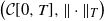 $\big(\mathcal C[0,T],\|\cdot\|_{T}\big)$
.
Using Lemma 1 and Kolmogorov’s continuity theorem (see, e.g., [Reference Khoshnevisan24, Theorem C.6]), there exist constants
 $\tau>0$
,
 $c_{3,10}>0$
, and
 $c_{3,11}>0$
such that, for all
 $n\ge c_{3,10}$
,
 $\mathbb E\big(\|\hat S_n\|_{T,\tau}^2\big) \le c_{3,11}$
. It follows from Chebyshev’s inequality that, for any
 $M>0$
,
 $\mathbb P\big(\|\hat S_n\|_{T,\tau} \ge M\big) \le {c_{3,11}}/{M^2}$
, which implies the tightness of
 $\{\hat S_n\}_{n\in\mathbb N_*}$
in
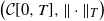 $\big(\mathcal C[0,T],\|\cdot\|_{T}\big)$
, since the Hölder space
 $\mathcal C^{\tau}[0,T]$
is compactly embedded in
 $\mathcal C[0,T]$
. The proof is complete.
4. Proof of Theorem 2
First, we apply the Gärtner–Ellis theorem [Reference Dembo and Zeitouni12, Theorem 2.3.6] to prove the MDP for the finite-dimensional distributions of
 $\{S_n\}_{n\in\mathbb N_{*}}$
; see Lemma 3. Then, we use the Dawson–Gärtner theorem [Reference Dembo and Zeitouni12, Section 4.6] to conclude sample-path MDP of
 $\{S_n\}_{n\in\mathbb N_{*}}$
in the topology of pointwise convergence; see Lemma 4. Finally, we strengthen the MDP to the topology of uniform convergence by establishing the exponential tightness of
 $\{S_n\}_{n\in\mathbb N_{*}}$
in
 $\big(\mathcal C[0,T],\|\cdot\|\big)$
; see Lemma 5. By combining all these results together, we obtain the sample-path MDP for
 $\{S_n\}_{n\in\mathbb N_{*}}$
in the space
 $\mathcal C[0,T]$
endowed with the topology of uniform convergence.
4.1. MDP of the finite-dimensional distributions
We first give the following formula for the exponential moment of S(t).
Lemma 2. Under the conditions of Theorem 2, for any
 $T>0$
there exists a constant
 $\theta_1>0$
such that, for any
 $|\theta|\le\theta_1$
and
 $t\in [0,T]$
,
 \begin{equation} \mathbb E\big[{\mathrm{e}}^{\theta S(t)}\big] = \exp\!\bigg(\int_{-\infty}^{t}\int_{-\infty}^{\infty}\bigg[ \exp\!\big(\theta\big(g(t-u)-g(\!-u)\big)r\big) - 1\bigg]\,{\mathrm{d}} F_u(r)\,{\mathrm{d}} u\bigg) < \infty. \end{equation}
Proof. Let
 $G(t,u, r) \,:\!= \big(g(t-u)-g(\!-u)\big)r$
. For any
 $M>0$
, let
 $$G_{(M)}(t,u,r) \,:\!= G(t,u,r)\cdot\mathbf{1}_{\{u\in[-M,t],|r|\le M\}},$$
and let
 $S_{(M)}(t) \,:\!= \int_{-\infty}^t\int_{-\infty}^{\infty}G_{(M)}(t,u,r)\,N({\mathrm{d}} u,{\mathrm{d}} r)$
,
 $t\ge 0$
. By Condition 1 and (6),
 $S_{(M)}(t)\rightarrow S(t)$
in
 $L^2(\Omega,\mathcal F,\mathbb P)$
and
 $G_{(M)}(t,\cdot,\cdot)\in L^1(\mathbb R^2,{\mathrm{d}} F_u(r)\,{\mathrm{d}} u)$
. Consequently, by Campbell’s theorem [Reference Kingman25, p. 28],
 \begin{equation} \log\mathbb E\big[\exp\!\big(\theta S_{(M)}(t)\big)\big] = \int_{-\infty}^t\int_{-\infty}^{\infty}\big[\exp\!(\theta G_{(M)}(t,u,r))-1\big]\,{\mathrm{d}} F_u(r)\,{\mathrm{d}} u \end{equation}
for any
 $\theta\in\mathbb R$
for which the integral on the right-hand side of (27) converges.
We claim that there exists a constant
 $\theta_1>0$
such that, for any
 $|\theta|\le \theta_1$
,
 \begin{equation} \int_{-\infty}^t\int_{-\infty}^{\infty}[\!\exp\!(\theta G(t,u,r)) - 1]\,{\mathrm{d}} F_u(r)\,{\mathrm{d}} u < \infty. \end{equation}
We postpone the proof of (28). Let us first prove (26).
Notice that
 $G_{(M)}(t,u,r)\rightarrow G(t,u,r)$
and
 $|G_{(M)}(t,u,r)|\le|G(t,u,r)|$
for any
 $t\ge0$
and
 $(u,r)\in\mathbb R^2$
. Thus, by (27), (28), and the dominated convergence theorem, we obtain (26).
Now we prove (28). For any
 $t\in [0,T]$
and
 $u\in\mathbb R$
, by (2),
 \begin{multline} \int_{-\infty}^{\infty}\big[\exp\!\big(\theta\big(g(t-u)-g(\!-u)\big)r\big) - 1\big]\,{\mathrm{d}} F_u(r) \\ = \int_{-\infty}^{\infty}\big[\exp\!\big(\theta\big(g(t-u)-g(\!-u)\big)r\big) - 1 - \theta \big(g(t-u)-g(\!-u)\big)r\big]\,{\mathrm{d}} F_u(r). \end{multline}
By using the elementary inequality
 \begin{equation} \big|{\mathrm{e}}^x-1-x\big| \le x^2{\mathrm{e}}^{|x|} \quad \text{for all } x \in \mathbb R, \end{equation}
and by using the Cauchy–Schwarz inequality, we obtain
 \begin{align} & \int_{-\infty}^{\infty}\big[\exp\!\big(\theta\big(g(t-u)-g(\!-u)\big)r\big) - 1 - \theta\big(g(t-u)-g(\!-u)\big)r\big]\,{\mathrm{d}} F_{u}(r) \nonumber \\ & \quad \le \theta^2\big(g(t-u)-g(\!-u)\big)^2\int_{-\infty}^{\infty}|r|^2 \exp\!\big(\theta\big|\big(g(t-u)-g(\!-u)\big)r\big|\big)\,{\mathrm{d}} F_{u}(r) \nonumber \\ & \quad \le \theta^2\big(g(t-u)-g(\!-u)\big)^2\bigg(\int_{-\infty}^{\infty}|r|^4\, {\mathrm{d}} F_{u}(r)\bigg)^{{1}/{2}} \nonumber \\ & \qquad \times \bigg(\int_{-\infty}^{\infty}\exp\!\big(2\theta\big|\big(g(t-u)-g(\!-u)\big)r\big|\big)\, {\mathrm{d}} F_{u}(r)\bigg)^{{1}/{2}}. \end{align}
By (4), we know that
 ${\sup}_{t\in[0,T],u\in\mathbb R}|g(t-u)-g(\!-u)| \le {\sup}_{t\in[0,T]}g(t) =: c_{g,T} < \infty$
. By using Condition 4, for any
 $\theta\le\theta_0/(2c_{g,T})$
and
 $u\in\mathbb R$
,
 \begin{equation} \int_{-\infty}^{\infty}\exp\!\big(2\theta|\big(g(t-u)-g(\!-u)\big)r|\big)\,{\mathrm{d}} F_{u}(r) \le \int_{-\infty}^{\infty}\exp\!(\theta_0|r|)\,{\mathrm{d}} F_{u}(r) \le M_{\theta_0}. \end{equation}
By (9), we obtain
 \begin{equation} \int_{-\infty}^t\big(g(t-u)-g(\!-u)\big)^2\bigg(\int_{-\infty}^{\infty}|r|^4\,{\mathrm{d}} F_{u}(r)\bigg)^{{1}/{2}}\,{\mathrm{d}} u \le \kappa^{1/2}\int_{-\infty}^t\big(g(t-u)-g(\!-u)\big)^2K_2(u)\,{\mathrm{d}} u, \end{equation}
which is finite by using Conditions 1 and 2, with
 $\gamma\in(0,1)$
and
 $\beta\in\big(\frac12-{\gamma}/{2},1\big)$
.
Putting (29)–(33) together, we obtain (28). The proof is complete.
For any
 $t\ge 0$
and
 $u\in\mathbb R\setminus\{0\}$
, let
 $g_{\beta,\gamma}(t,u) \,:\!= \big((t-u)_+^{1-\beta}-(-u)_+^{1-\beta}\big)|u|^{-{\gamma}/{2}}$
. For any
 $\boldsymbol{t}=(t_1,\ldots,t_m)^\top\in \mathbb R_+^m$
, let
 $M_{\beta,\gamma}(\boldsymbol{t})\,:\!=\big(M_{\beta,\gamma}(t_i,t_j)\big)_{i,j\in\{1,\ldots,m\}}$
be the
 $m\times m$
matrix with entries
 $M_{\beta,\gamma}(t_i,t_j)\,:\!=\int_{\mathbb R}g_{\beta,\gamma}(t_i,u)g_{\beta,\gamma}(t_j,u)\,{\mathrm{d}} u$
.
Lemma 3. Under the conditions of Theorem 2, for any
 $m\in\mathbb N$
,
 ${\boldsymbol\theta}=(\theta_1,\ldots,\theta_m)^\top\in\mathbb R^m$
and
 $\boldsymbol{t}=(t_1,\ldots,t_m)^\top\in\mathbb R_+^m$
, the following limit exists:
 \begin{equation} \lim_{n\rightarrow\infty}\frac{1}{\pi(n)^2}\log\mathbb E\Bigg[ \exp\!\Bigg(\pi(n)^2\sum_{i=1}^m\theta_iS_n(t_i)\Bigg)\Bigg] = \frac{1}{2}\left\langle{\boldsymbol\theta},M_{\beta,\gamma}(\boldsymbol{t}){\boldsymbol \theta}\right\rangle. \end{equation}
Consequently, as
 $n\rightarrow\infty$
, the sequence
 $\{(S_n(t_1),\ldots,S_n(t_m))\}_{n\in\mathbb N_*}$
satisfies a large deviation principle on
 $\mathbb R^m$
with speed function
 $\pi(n)^2$
and rate function
 $J^{M_{\beta,\gamma}(\boldsymbol{t})}$
defined for
 ${\boldsymbol{x}}\in\mathbb R^m$
by
 $$J^{M_{\beta,\gamma}(\boldsymbol{t})}(\boldsymbol{x}) \,:\!= {\sup}_{\boldsymbol{y}\in\mathbb R^m}\bigg\{ {\boldsymbol{x}}^\top{\boldsymbol{y}}-\frac12{\boldsymbol{y}}^\top M_{\beta,\gamma}(\boldsymbol{t}){\boldsymbol{y}}\bigg\}.$$
Proof. First, let us state the following two facts, which will be used frequently:
-
(i) Under Conditions 2, 3, and 6, it follows from (22) that
(35)
\begin{equation} \lim_{n\rightarrow\infty}{\sup}_{-\infty < u\le t\le T}\frac{\pi(n)}{b(n)}|g(nt -nu)-g(\!-nu)| = 0. \end{equation}
-
(ii) Under Conditions 2, 3, and 4, we derive, as in [Reference Pang and Taqqu35, (52)], that
(36)Furthermore, it follows from the dominated convergence theorem, (23), and (36) that
\begin{equation} \lim_{n\rightarrow\infty}\frac{n}{b(n)^2}\big(g(nt -nu)-g(\!-nu)\big)^2 K_2(nu) = \big((t-u)_+^{1-\beta}-(\!-u)_+^{1-\beta}\big)^2|u|^{-\gamma}. \end{equation}
(37)
\begin{multline} \lim_{n\rightarrow\infty}\int_{-\infty}^t\frac{n}{b(n)^2}\big(g(nt-nu)-g(\!-nu)\big)^2K_2(nu)\,{\mathrm{d}} u \\ = \int_{-\infty}^t\big((t-u)_+^{1-\beta}-(\!-u)_+^{1-\beta}\big)^2|u|^{-\gamma}\,{\mathrm{d}} u. \end{multline}


We first prove (34) in the case
 $m=1$
, that is,
 \begin{equation} \lim_{n\rightarrow\infty}\frac{1}{\pi(n)^2}\log\mathbb E[\exp\!(\theta\pi(n)^2S_n(t))] = \frac{\theta^2}{2}\int_{-\infty}^t\big((t-u)_+^{1-\beta}-(\!-u)_+^{1-\beta}\big)^2|u|^{-\gamma}\,{\mathrm{d}} u. \end{equation}
The proof of (38) is divided into two parts: the upper bound and the lower bound.
Step 1: Upper bound. For any fixed
 $\theta\in\mathbb R$
,
 $t\ge0$
, by (2), (26), and (35), we have
 \begin{align} & \frac{1}{\pi(n)^2}\log\mathbb E[\exp\!(\theta\pi(n)^2S_n(t))] \nonumber \\ & \qquad = \frac{1}{\pi^{2}(n)}\int_{-\infty}^{at}\int_{\mathbb R}\bigg[ \exp\!\bigg(\theta\frac{\pi(n)}{b(n)}\big(g(nt-u)-g(\!-u)\big)r\bigg) - 1\bigg]\,{\mathrm{d}} F_u(r)\,{\mathrm{d}} u \nonumber \\ & \qquad = \frac{1}{\pi^{2}(n)}\int_{-\infty}^t\int_{\mathbb R}\bigg[ \exp\!\bigg(\theta\frac{\pi(n)}{b(n)}\big(g(nt-nu)-g(\!-nu)\big)r\bigg) - 1 \nonumber \\ & \qquad\qquad\qquad\qquad\qquad - \theta\frac{\pi(n)}{b(n)}\big(g(nt-nu)-g(\!-nu)\big)r\bigg]\,{\mathrm{d}} F_{nu}(r)\,n{\mathrm{d}} u. \end{align}
For any
 $\varepsilon>0$
, there exists a constant
 $c_{4,1}(\varepsilon)>0$
such that
 \begin{equation} \bigg|{\mathrm{e}}^{x}-1-x-\frac{x^2}{2}\bigg| \le \frac{\varepsilon}{2}x^2 \quad \text{for all } |x| \le c_{4,1}(\varepsilon). \end{equation}
It follows from (35) and (40) that, for any
 $\varepsilon>0$
and
 $r_0>0$
,
 \begin{align} & \limsup_{n\rightarrow\infty}\frac{1}{\pi^{2}(n)}\bigg(\int_{-\infty}^t\int_{|r|\le r_0}\bigg[ \exp\!\bigg(\theta\frac{\pi(n)}{b(n)}\big(g(nt-nu)-g(\!-nu)\big)r\bigg) - 1 \nonumber \\ & \qquad\qquad\qquad\qquad\qquad\qquad - \theta\frac{\pi(n)}{b(n)}\big(g(nt-nu)-g(\!-nu)\big)r\bigg]\,{\mathrm{d}} F_{nu}(r)\,n{\mathrm{d}} u\bigg) \nonumber \\ & \qquad \le \frac{(1+\varepsilon)\theta^2}{2}\limsup_{n\rightarrow\infty}\int_{-\infty}^t\int_{|r|\le r_0}\frac{n}{b(n)^2} \big(g(nt-nu)-g(\!-nu)\big)^2r^2\,{\mathrm{d}} F_{nu}(r)\,{\mathrm{d}} u \nonumber \\ & \qquad \le \frac{(1+\varepsilon)\theta^2}{2}\lim_{n\rightarrow\infty}\int_{-\infty}^t\frac{n}{b(n)^2} \big(g(nt-nu)-g(\!-nu)\big)^2K_2(nu)\,{\mathrm{d}} u \nonumber \\ & \qquad = \frac{(1+\varepsilon)\theta^2}{2}\int_{-\infty}^t\big((t-u)_+^{1-\beta}-(\!-u)_+^{1-\beta}\big)^2 |u|^{-\gamma}\,{\mathrm{d}} u, \end{align}
where (37) was used in the last step.
It follows from (30) and the Cauchy–Schwarz inequality that
 \begin{align} & \int_{|r|>r_0}\!\bigg[\exp\!\bigg(\theta\frac{\pi(n)}{b(n)}\big(g(nt-nu)-g(\!-nu)\big)r\bigg) - 1 - \theta\frac{\pi(n)}{b(n)}\big(g(nt-nu)-g(\!-nu)\big)r\bigg]\,{\mathrm{d}} F_{nu}(r) \nonumber \\ & \le \theta^2\frac{\pi(n)^2}{b(n)^2}\big(g(nt-nu)-g(\!-nu)\big)^2\!\int_{|r|>r_0}|r|^2 \exp\!\bigg(\theta\frac{\pi(n)}{b(n)}|\big(g(nt-nu)-g(\!-nu)\big)r|\bigg)\,{\mathrm{d}} F_{nu}(r) \nonumber \\ & \le \theta^2\frac{\pi(n)^2}{b(n)^2}\big(g(nt-nu)-g(\!-nu)\big)^2 \bigg(\int_{\mathbb R}|r|^4\,{\mathrm{d}} F_{nu}(r)\bigg)^{{1}/{2}} \nonumber \\ & \quad \times \bigg(\int_{|r|>r_0}\exp\!\bigg(2\theta\frac{\pi(n)}{b(n)}|\big(g(nt-nu)-g(\!-nu)\big)r|\bigg)\, {\mathrm{d}} F_{nu}(r)\bigg)^{{1}/{2}}. \end{align}
By (35) and Chebyshev’s inequality we have, for sufficiently large n,
 \begin{align} & \int_{|r|>r_0}\exp\!\bigg(2\theta\frac{\pi(n)}{b(n)}|\big(g(nt-nu)-g(\!-nu)\big)r|\bigg)\,{\mathrm{d}} F_{nu}(r)\nonumber\\ & \qquad \le \int_{|r|>r_0}\exp\!\bigg(\frac{\theta_0}{2}|r|\bigg)\,{\mathrm{d}} F_{nu}(r) \nonumber \\ & \qquad \le \exp\!\bigg({-}\frac{\theta_0r_0}{2}\bigg)\int_{|r|>r_0}\exp\!(\theta_0|r|)\,{\mathrm{d}} F_{nu}(r) \le \exp\!\bigg({-}\frac{\theta_0r_0}{2}\bigg)M_{\theta_0}, \end{align}
where (8) in Condition 4 was used in the last step.
By using Condition 5 and (37), we derive
 \begin{align} & \limsup_{n\rightarrow\infty}\frac{n}{b(n)^2}\int_{-\infty}^t\big(g(nt-nu)-g(\!-nu)\big)^2 \bigg(\int_{\mathbb R}|r|^4\,{\mathrm{d}} F_{nu}(r)\bigg)^{{1}/{2}}\,{\mathrm{d}} u \nonumber \\ & \qquad = \limsup_{n\rightarrow\infty}\frac{n}{b(n)^2}\int_{-\infty}^t\big(g(nt-nu)-g(\!-nu)\big)^2 K_4(nu)^{{1}/{2}}\,{\mathrm{d}} u \nonumber \\ & \qquad \le \kappa^{1/2}\limsup_{n\rightarrow\infty}\frac{n}{b(n)^2}\int_{-\infty}^t\big(g(nt-nu)-g(\!-nu)\big)^2 K_2(nu)\,{\mathrm{d}} u \nonumber \\ & \qquad = \kappa^{1/2}\int_{-\infty}^t\big((t-u)_{+}^{1-\beta}-(\!-u)_+^{1-\beta}\big)^2|u|^{-\gamma}\,{\mathrm{d}} u. \end{align}
Putting (39), (41), (42), (43), and (44) together, and using the arbitrariness of
 $r_0$
, we obtain that, for any
 $\theta\in\mathbb R$
,
 $t\ge0$
, and
 $\varepsilon\in(0,1)$
,
 \begin{multline} \limsup_{n\rightarrow\infty}\frac{1}{\pi(n)^2}\log\mathbb E[\!\exp\!(\theta\pi(n)^2S_n(t))] \\ \le \frac{\theta^2(1+\varepsilon)}{2}\int_{-\infty}^t\big((t-u)_+^{1-\beta}-(\!-u)_+^{1-\beta}\big)^2|u|^{-\gamma}\,{\mathrm{d}} u. \end{multline}
Step 2: Lower bound. Since
 ${\mathrm{e}}^{x}-1-x \geq 0$
for all
 $x\in\mathbb R$
, it follows from (35) and (40) that, for any
 $\varepsilon\in (0,1)$
and
 $r_0>0$
,
 \begin{align} & \liminf_{n\rightarrow\infty}\frac{1}{\pi^{2}(n)}\bigg(\int_{-\infty}^t\int_{\mathbb R}\bigg[ \exp\!\bigg(\theta\frac{\pi(n)}{b(n)}\big(g(nt-nu)-g(\!-nu)\big)r\bigg) - 1 \nonumber \\ & \qquad\qquad\qquad\qquad\qquad -\theta\frac{\pi(n)}{b(n)}\big(g(nt-nu)-g(\!-nu)\big)r\bigg]\,{\mathrm{d}} F_{nu}(r)\,n{\mathrm{d}} u\bigg) \nonumber \\ & \geq \liminf_{n\rightarrow\infty}\frac{1}{\pi^{2}(n)}\bigg(\int_{-\infty}^t\int_{|r|\le r_0}\bigg[ \exp\!\bigg(\theta\frac{\pi(n)}{b(n)}\big(g(nt-nu)-g(\!-nu)\big)r\bigg) - 1 \nonumber \\ & \qquad\qquad\qquad\qquad\qquad\qquad\quad -\theta\frac{\pi(n)}{b(n)}\big(g(nt-nu)-g(\!-nu)\big)r\bigg]\,{\mathrm{d}} F_{nu}(r)\,n{\mathrm{d}} u\bigg) \nonumber \\ & \geq \frac{(1-\varepsilon)\theta^2}{2}\liminf_{n\rightarrow\infty}\int_{-\infty}^t\int_{|r|\le r_0}\frac{n}{b(n)^2} \big(g(nt-nu)-g(\!-nu)\big)^2r^2\,{\mathrm{d}} F_{nu}(r)\,{\mathrm{d}} u \nonumber \\ & \geq \frac{(1-\varepsilon)\theta^2}{2}\liminf_{n\rightarrow\infty}\int_{-\infty}^t\int_{\mathbb R}\frac{n}{b(n)^2} \big(g(nt-nu)-g(\!-nu)\big)^2K_2(nu)\,{\mathrm{d}} u \nonumber \\ & \quad - \frac{(1-\varepsilon)\theta^2}{2}\limsup_{n\rightarrow\infty}\int_{-\infty}^t\int_{|r|>r_0}\frac{n}{b(n)^2} \big(g(nt-nu)-g(\!-nu)\big)^2r^2\,{\mathrm{d}} F_{nu}(r)\,{\mathrm{d}} u \nonumber \\ & = \frac{(1-\varepsilon)\theta^2}{2}\int_{-\infty}^t\big((t-u)_+^{1-\beta}-(\!-u)_+^{1-\beta}\big)^2 |u|^{-\gamma}\,{\mathrm{d}} u \nonumber \\ & \quad - \frac{(1-\varepsilon)\theta^2}{2}\limsup_{n\rightarrow\infty}\int_{-\infty}^t\int_{|r|>r_0}\frac{n}{b(n)^2} \big(g(nt-nu)-g(\!-nu)\big)^2r^2\,{\mathrm{d}} F_{nu}(r)\,{\mathrm{d}} u, \end{align}
where (37) was used in the last step. Next, we prove that the last term in (46) can be ignored as
 $r_0\to \infty$
.
By using the Cauchy–Schwarz inequality and Condition 5, we have
 \begin{align} & \int_{-\infty}^t\int_{|r|>r_0}\frac{n}{b(n)^2}\big(g(nt-nu)-g(\!-nu)\big)^2r^2\,{\mathrm{d}} F_{nu}(r)\,{\mathrm{d}} u \nonumber \\ & \quad \le \frac{n}{b(n)^2}\int_{-\infty}^t\big(g(nt-nu)-g(\!-nu)\big)^2 \bigg(\int_{\mathbb R}|r|^4\,{\mathrm{d}} F_{nu}(r)\bigg)^{{1}/{2}} \bigg(\int_{|r|>r_0}\,{\mathrm{d}} F_{nu}(r)\bigg)^{{1}/{2}}\,{\mathrm{d}} u \nonumber \\ & \quad \le \frac{\kappa^{1/2}n}{b(n)^2}\int_{-\infty}^t\big(g(nt-nu)-g(\!-nu)\big)^2K_2(nu)\,{\mathrm{d}} u \cdot {\sup}_{u\in\mathbb R}\bigg(\int_{|r|>r_0}\,{\mathrm{d}} F_{nu}(r)\bigg)^{{1}/{2}}. \end{align}
By Chebyshev’s inequality and Condition 4, we have
 \begin{align} {\sup}_{u\in\mathbb R}\int_{|r|>r_0}{\mathrm{d}} F_{nu}(r) & \le \exp\!(\!-\theta_0r_0) \cdot {\sup}_{u\in\mathbb R}\int_{|r|>r_0}\exp\!(\theta_0|r|)\,{\mathrm{d}} F_{nu}(r) \nonumber \\ & \le \exp\!(\!-\theta_0r_0)M_{\theta_0}. \end{align}
Putting (39), (46), (47), and (48) together, and using the arbitrariness of
 $r_0$
, we obtain that, for any
 $\theta\in\mathbb R$
,
 $t\ge0$
, and
 $\varepsilon\in(0,1)$
,
 \begin{equation*} \liminf_{n\rightarrow\infty}\frac{1}{\pi(n)^2}\log\mathbb E[\exp\!(\theta\pi(n)^2S_n(t))] \ge \frac{\theta^2(1-\varepsilon)}{2}\int_{-\infty}^t\big((t-u)_+^{1-\beta}-(\!-u)_+^{1-\beta}\big)^2|u|^{-\gamma}\,{\mathrm{d}} u. \end{equation*}
This, together with (45), implies (38).
Next, we prove (34) for
 $m\ge2$
. Notice that, for any
 ${\boldsymbol{\theta}}\,:\!=(\theta_1,\ldots,\theta_m)^\top\in\mathbb R^m$
and
 $\boldsymbol{t}\,:\!=(t_1,\ldots,t_m)^\top\in\mathbb R_+^m$
, we can write
 \begin{multline*} \mathbb E\Bigg[\exp\!\Bigg(\frac{\pi(n)}{b(n)}\sum_{i=1}^m\theta_iS(nt_i)\Bigg)\Bigg] \\ = \mathbb E\Bigg[\exp\!\Bigg(\frac{\pi(n)}{b(n)}\int_{\mathbb R}\int_{\mathbb R} \Bigg(\sum_{j=1}^k\theta_j\big(g(nt_j-u)-g(\!-u)\big)\Bigg)r\,N({\mathrm{d}} u,{\mathrm{d}} r)\Bigg)\Bigg]. \end{multline*}
The proof of (34) is similar to that of (38). More specifically, we replace
 $\theta\big(g(nt-u)-g(\!-u)\big)$
in (39) and (46) with
 $\sum_{j=1}^m\theta_j\big(g(nt_j-u)-g(\!-u)\big)$
and follow the same computation to obtain
 \begin{align*} & \lim_{n\rightarrow\infty}\frac{1}{\pi(n)^2}\log\mathbb E\Bigg[ \exp\!\Bigg(\pi(n)^2\sum_{i=1}^m\theta_iS_n(t_i)\Bigg)\Bigg] \\ & \qquad = \frac12\int_{-\infty}^{\infty}\Bigg(\sum_{j=1}^m\theta_j\big((t_j-u)_+^{1-\beta}-(\!-u)_+^{1-\beta}\big)\Bigg)^2 |u|^{-\gamma}\,{\mathrm{d}} u \\ & \qquad = \frac12\big\langle{\boldsymbol{\theta}},M_{\beta,\gamma}({\boldsymbol{t}}){\boldsymbol{\theta}}\big\rangle. \end{align*}
Thus, (34) holds. By the Gärtner–Ellis theorem (see, e.g., [Reference Dembo and Zeitouni12, Theorem 2.3.6]), we obtain the desired result.
4.2. MDP in the topology of pointwise convergence
Lemma 4. Under the conditions of Theorem 2,
 $\{S_n(t)\colon t\in[0,T]\}_{n\in\mathbb N_*}$
satisfies a large deviation principle on
 $\mathcal C[0,T]$
in the topology of pointwise convergence as
 $n\rightarrow\infty$
, with speed function
 $\pi(n)^2$
and the rate function
 $I_{\beta,\gamma}$
given by (11).
Proof. It follows from the Dawson–Gärtner theorem [Reference Dembo and Zeitouni12, Theorem 4.6.1] and Lemma 3 that the family
 $\{S_n(t)\colon t\in[0,T]\}_{n\in\mathbb N_*}$
satisfies a large deviation principle on
 $\mathcal C[0,T]$
in the topology of pointwise convergence as
 $n\rightarrow\infty$
, with the speed function
 $\pi(n)^2$
and the rate function
 $I_{\beta,\gamma}'$
given by
 \begin{equation} I_{\beta,\gamma}'(\xi) \,:\!= {\sup}_{0\le t_1 < \cdots < t_m\le T,m\in\mathbb N}J^{M_{\beta,\gamma}(t_1,\ldots,t_m)} ((\xi(t_1),\ldots,\xi_{t_m})^\top). \end{equation}
Following exactly the same steps as in the proof of [Reference Majewski33, Lemma 11], we conclude that the rate functions
 $I'_{\beta,\gamma}$
in (49) and
 $I_{\beta,\gamma}$
in (11) agree on
 $\mathcal C[0,T]$
. The proof is complete.
4.3. Exponential tightness in
$\big(\mathcal C[0, T], \|\cdot\|_T\big)$
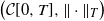
To strengthen the MDP to the topology of uniform convergence, we establish the associated exponential tightness of
 $\{S_n(t)\colon t\in[0,T]\}_{n\in\mathbb N_*}$
.
Lemma 5. Under the conditions of Theorem 2, for any
 $M>0$
there exists a compact set
 $\mathcal K_M \subset \big(\mathcal C[0,T], \|\cdot\|_T\big)$
such that
 $\limsup_{n\rightarrow\infty}(1/{\pi(n)^2})\log\mathbb P(S_n\notin\mathcal K_M) \le -M$
.
Lemma 6. Under the conditions of Theorem 2, for any
 $T>0$
there exist some positive constants
 $c_{4,2}$
,
 $c_{4,3}$
, and
 $c_{4,4}$
such that, for any
 $n\ge c_{4,2}$
, and
 $0\le s$
,
 $t\le T$
, with
 $0 < \eta < \frac{3}{2}-\beta-{\gamma}/{2}$
, the following inequality holds:
 \begin{equation} \mathbb E\bigg[\exp\!\bigg(\pi(n)^2\frac{|S_n(t)-S_n(s)|}{|t-s|^{\eta}}\bigg)\bigg] \le c_{4,3}\exp\!(c_{4,4}\pi(n)^2). \end{equation}
Proof. By using the same argument as in the proof of (38) we obtain, for any
 $\theta\in\mathbb R$
and
 $0\le s< t\le T$
,
 \begin{align} \lim_{n\rightarrow\infty}\frac{1}{\pi(n)^2}\log\mathbb E[\exp\!(\theta\pi(n)^2(S_n(t)-S_n(s))] & = \frac{\theta^2}{2}\int_{-\infty}^t \big((t-u)_+^{1-\beta}-(s-u)_+^{1-\beta}\big)^2|u|^{-\gamma}\,{\mathrm{d}} u \nonumber \\ & \le c_{2,1}(\gamma,\beta)\frac{\theta^2}{2}|t-s|^{3-2\beta-\gamma}, \end{align}
where (7) was used in the last step. Taking
 $\theta=\pm{1}/{|t-s|^{\eta}}$
in (51), we have
 \begin{align*} & \limsup_{n\rightarrow\infty}\frac{1}{\pi(n)^2}\log\mathbb E\bigg[ \exp\!\bigg(\pi(n)^2\frac{|S_n(t)-S_n(s)|}{|t-s|^{\eta}}\bigg)\bigg] \\ & \qquad = \max\bigg\{\lim_{n\rightarrow\infty}\frac{1}{\pi(n)^2}\log\mathbb E\bigg[ \exp\!\bigg(\pi(n)^2\frac{S_n(t)-S_n(s)}{|t-s|^{\eta}}\bigg)\bigg], \\ & \qquad\qquad\quad\ \ \lim_{n\rightarrow\infty}\frac{1}{\pi(n)^2}\log\mathbb E\bigg[ \exp\!\bigg({-}\pi(n)^2\frac{S_n(t)-S_n(s)}{|t-s|^{\eta}}\bigg)\bigg]\bigg\} \\ & \qquad \le c_{2,1}(\gamma,\beta)|t-s|^{3-2\beta-\gamma-2\eta}. \end{align*}
This implies (50). The proof is complete.
5. Proofs of Propositions 1 and 2
Proof of Proposition 1. The proof for (15) follows the same lines as the proof of [Reference Chang, Yao and Zajic10, Lemma 5.2] or [Reference Anugu and Pang1, Lemma 4.1], and the proof for (16) follows that of [Reference Chang, Yao and Zajic10, Theorem 4.1] or [Reference Anugu and Pang1, Theorem 4.1]. We adopt the same approach for our process. To save space, we provide the details only for the proof of (15), while (16) can be proved using a similar argument.
Let
 $M_{n}(t)\,:\!=M(nt)/n$
. Take
 $\pi(n)=n/b(n)$
. Then Condition 6 holds by the choice of
 $\beta \in \big(\frac12-{\gamma}/{2},1-\gamma\big)$
. Clearly,
 \begin{equation*} M_{n}(t) = \frac{{\sup}_{0\le s\le nt}(S(s)-\nu s)}{n} = {\sup}_{0\le s\le t}(S_n(s) -\nu s). \end{equation*}
Since the mapping
 $\{S_n(t)\}_{t\in[0,1]}\in\mathcal C[0,1] \mapsto \{M_n(t)\}_{t\in[0,1]}\in\mathcal C[0,1]$
is continuous, it follows from the contraction principle that
 $\{M_n(t)\colon t\in[0,1]\}_{n\in\mathbb N_*}$
satisfies the LDP with speed
 $n^2/b(n)^2$
and a good rate function
 $I_M(\psi)\colon \mathcal C[0,1] \rightarrow \mathbb R$
given by
 \begin{align*} I_M(\psi) \,:\!= \inf\bigg\{ & I_{\beta,\gamma}(\phi)\colon \text{for all } t\in[0,1], \\ & {\sup}_{0\le s\le t}\bigg[\int_{-\infty}^s\big((s-u)_+^{1-\beta}-(\!-u)_+^{1-\beta}\big)|u|^{-{\gamma}/{2}}\phi(u)\,{\mathrm{d}} u - \nu s\bigg] = \psi(t)\bigg\}, \end{align*}
where
 $I_{\beta,\gamma}$
is given by (11). In addition, from the contraction principle and
 $M_n(1)=M(n)/n$
, we know that
 $\{M(n)/n\}_{n\in\mathbb N_*}$
satisfies the LDP with speed
 $n^2/b(n)^2$
and a good rate function
 $\Lambda^*_M(\lambda)=\inf_{\psi(1)=\lambda}I_M(\psi)$
. In particular,
 \begin{equation*} \limsup_{n\rightarrow\infty}\frac{b(n)^2}{n^2}\log\mathbb P\bigg(\frac{M(n)}{n} > \lambda\bigg) \le -\inf_{x>\lambda}\Lambda^*_M(x) = -\inf_{\phi\in\mathcal G_1}\int_{-\infty}^1\frac{1}{2}\phi(u)^2\,{\mathrm{d}} u, \end{equation*}
where
 $$ \mathcal G_1 = \bigg\{\phi\in L^2((\!-\infty,1])\colon {\sup}_{0\le s\le 1}\bigg[ \int_{-\infty}^s\big((s-u)_+^{1-\beta}-(\!-u)_+^{1-\beta}\big)|u|^{-{\gamma}/{2}}\phi(u)\,{\mathrm{d}} u - \nu s\bigg] > \lambda\bigg\}. $$
Now, define
 $$ \mathcal G_s = \bigg\{\phi\in L^2((\!-\infty,s])\colon\bigg[ \int_{-\infty}^s\big((s-u)_+^{1-\beta}-(\!-u)_+^{1-\beta}\big)|u|^{-{\gamma}/{2}}\phi(u)\,{\mathrm{d}} u - \nu s\bigg] > \lambda\bigg\}. $$
Then,
 $\mathcal G_1=\cup_{0\le s\le 1}\mathcal G_s$
. By Lemma 8(i),
 $$\inf_{\phi\in\mathcal G_s}\int_{-\infty}^s\phi(u)^2\,{\mathrm{d}} u = \frac{(\nu s+\lambda)^2}{c_{\beta,\gamma}s^{2H}}.$$
Note that
 $\inf_{\phi\in\mathcal G_s}\int_{-\infty}^1\phi(u)^2\,{\mathrm{d}} u = \inf_{\phi\in\mathcal G_s}\int_{-\infty}^s\phi(u)^2\,{\mathrm{d}} u$
, since we can simply set
 $\phi(u)=0$
for
 $s < u\le 1$
. Hence,
 \begin{equation*} \inf_{\phi\in\mathcal G_1}\int_{-\infty}^1\phi(u)^2\,{\mathrm{d}} u = \inf_{0\le s\le1}\inf_{\phi\in\mathcal G_s} \int_{-\infty}^1\phi(u)^2\,{\mathrm{d}} u = \inf_{0\le s\le1}\frac{(\nu s+\lambda)^2}{c_{\beta,\gamma}s^{2H}}. \end{equation*}
To solve the above minimization problem, it suffices to minimize the function
 $f(s)\,:\!=({\nu s+\lambda})/{s^H}$
. It is easy to verify that f’(s) has a single zero at
 $s^*={H\lambda}/{\nu(1-H)}$
, and that f(s) is decreasing for
 $s < s^*$
and increasing for
 $s > s^*$
. Hence, when
 $\lambda<\nu(1-H)/H$
the optimal solution is
 $s=s^*<1$
, and when
 $\lambda\ge\nu(1-H)/H$
the optimal solution is
 $s=1$
.
The desired optimal value
 $\mathcal I(\lambda)$
follows. Therefore, we have proved that
 $$ \limsup_{n\rightarrow\infty}\frac{b(n)^2}{n^2}\log\mathbb P\bigg(\frac{M(n)}{n} > \lambda\bigg) \le -\mathcal I(\lambda). $$
Analogously, we can prove that
 $$ \liminf_{n\rightarrow\infty}\frac{b(n)^2}{n^2}\log\mathbb P\bigg(\frac{M(n)}{n} > \lambda\bigg) \ge -\mathcal I(\lambda). $$
Thus, the proof is complete.
Proof of Proposition 2. This proposition can be proved along exactly the same lines as the proof of [Reference Chang, Yao and Zajic10, Theorem 5.1]. To save space, the details are omitted.
6. Proof of Theorem 3
Proof of Theorem 3. The absence of Condition 5 makes the situation slightly different. For the reader’s convenience, we provide a self-contained proof of (38) under Conditions 1–4 and 7. The proofs for the remaining results in Lemmas 2, 3, and 5, and Theorem 2, follow similarly to those in Section 4, and are therefore omitted.
Step 1: Upper bound. Under Conditions 3 and 7, by using Potter’s theorem (see (21)) and the procedure as in (22), there exist constants
 $c_{6,1}, c_{6,2}\in (0,\infty)$
such that, for every
 $n\ge c_{6,1}$
,
 \begin{equation} \frac{\pi(n)}{b(n)}|g(nt-nu)-g(\!-nu)| \leq c_{6,2}{n^{-\eta/2}} \quad \hbox{for all } -\infty< u\le t\le T. \end{equation}
Recall the constant
 $c_{4,1}(\varepsilon)$
from (40) for any fixed
 $\varepsilon>0$
. By (36), (40), and (52), we have
 \begin{align} & \limsup_{n\rightarrow\infty}\frac{1}{\pi^{2}(n)}\bigg( \int^{t}_{-\infty}\int_{|r|\le\frac{c_{4,1}(\varepsilon)n^{\eta/2}}{\theta c_{6,2}}}\bigg[ \exp\!\bigg(\theta\frac{\pi(n)}{b(n)}\big(g(nt-nu)-g(\!-nu)\big)r\bigg) - 1 \nonumber \\ & \qquad\qquad\qquad\qquad\qquad\qquad\qquad\quad - \theta\frac{\pi(n)}{b(n)}\big(g(nt-nu)-g(\!-nu)\big)r\bigg]\,{\mathrm{d}} F_{nu}(r)\,n{\mathrm{d}} u\bigg) \nonumber \\ & \le \frac{(1+\varepsilon)\theta^2n}{2b(n)^2}\limsup_{n\rightarrow\infty} \int_{-\infty}^t\int_{|r|\le\frac{c_{4,1}(\varepsilon)n^{\eta/2}}{\theta c_{6,2}}}\big(g(nt-nu)-g(\!-nu)\big)^2 r^2\,{\mathrm{d}} F_{nu}(r)\,{\mathrm{d}} u \nonumber \\ & \le \frac{(1+\varepsilon)\theta^2n}{2b(n)^2}\lim_{n\rightarrow\infty}\int_{-\infty}^t\big(g(nt-nu)-g(\!-nu)\big)^2 K_2(nu)\,{\mathrm{d}} u \nonumber \\ & = \frac{(1+\varepsilon)\theta^2}{2}\int_{-\infty}^t\big((t-u)_+^{1-\beta}-(\!-u)_+^{1-\beta}\big)^2 |u|^{-\gamma}\,{\mathrm{d}} u. \end{align}
By (30) and Hölder’s inequality, we obtain that, for any
 $p\in (1,{\gamma}/{(1-2\beta)_+})$
,
 \begin{align*} & \int_{|r|>\frac{c_{4,1}(\varepsilon)n^{\eta/2}}{\theta c_{6,2}}}\bigg[ \exp\!\bigg(\theta\frac{\pi(n)}{b(n)}\big(g(nt-nu)-g(\!-nu)\big)r\bigg) - 1 \\ & \qquad\qquad\qquad\ -\theta\frac{\pi(n)}{b(n)}\big(g(nt-nu)-g(\!-nu)\big)r\bigg]\,{\mathrm{d}} F_{nu}(r) \\ & \le \theta^2\frac{\pi(n)^2}{b(n)^2}\big(g(nt-nu)-g(\!-nu)\big)^2 \\ & \quad \times \int_{|r|>\frac{c_{4,1}(\varepsilon)n^{\eta/2}}{\theta c_{6,2}}}|r|^2 \exp\!\bigg(\theta\frac{\pi(n)}{b(n)}|\big(g(nt-nu)-g(\!-nu)\big)r|\bigg)\,{\mathrm{d}} F_{nu}(r) \\ & \le \theta^2\frac{\pi(n)^2}{b(n)^2}\big(g(nt-nu)-g(\!-nu)\big)^2\bigg( \int_{\mathbb R}|r|^2\,{\mathrm{d}} F_{nu}(r)\bigg)^{{1}/{p}} \\ & \quad \times \Bigg(\int_{|r|>\frac{c_{4,1}(\varepsilon)n^{\eta/2}}{\theta c_{6,2}}}|r|^2 \exp\!\bigg(\frac{p\theta}{p-1}\cdot\frac{\pi(n)}{b(n)}|\big(g(nt-nu)-g(\!-nu)\big)r|\bigg)\, {\mathrm{d}} F_{nu}(r)\Bigg)^{({p-1})/{p}}. \end{align*}
For every fixed
 $\theta\in\mathbb R$
and
 $p\in(1,{\gamma}/{(1-2\beta)_+})$
, by (52), there exists a constant
 $c_{6,3}>0$
such that, for every
 $n\ge c_{6,3}$
,
 $$ \frac{p|\theta|}{p-1}\cdot\frac{\pi(n)}{b(n)}|(g(nt-nu)-g(\!-nu)| \leq \frac{\theta_0}{4} \quad \text{for all } -\infty < u\le t\le T. $$
This, together with the elementary inequality
 \begin{equation} x^2 \le 2c^{-2}{\mathrm{e}}^{c|x|} \quad \text{for every } c\ge0,\, x\in \mathbb R, \end{equation}
implies that
 \begin{align} & \int_{|r|>\frac{c_{4,1}(\varepsilon)n^{\eta/2}}{\theta c_{6,2}}}|r|^2\exp\!\bigg( \frac{p\theta}{p-1}\cdot\frac{\pi(n)}{b(n)}\big|\big(g(nt-nu)-g(\!-nu)\big)r\big|\bigg)\, {\mathrm{d}} F_{nu}(r) \nonumber \\ & \qquad \le \int_{|r|>\frac{c_{4,1}(\varepsilon)n^{\eta/2}}{\theta c_{6,2}}}|r|^2\exp\!\bigg( \frac{\theta_0}{4}|r|\bigg)\,{\mathrm{d}} F_{nu}(r) \nonumber \\ & \qquad \le 32\theta_0^{-2}\int_{|r|>\frac{c_{4,1}(\varepsilon)n^{\eta/2}}{\theta c_{6,2}}}\exp\!\bigg( \frac{\theta_0}{2}|r|\bigg)\,{\mathrm{d}} F_{nu}(r) \nonumber \\ & \qquad \le 32\theta_0^{-2}\exp\!\bigg({-}\frac{\theta_0}{2} \frac{c_{4,1}(\varepsilon)n^{\eta/2}}{\theta c_{6,2}}\bigg)\Bigg( \int_{|r|>\frac{c_{4,1}(\varepsilon)n^{\eta/2}}{\theta c_{6,2}}}\exp\!(\theta_0|r|)\,{\mathrm{d}} F_{nu}(r)\Bigg) \nonumber \\ & \qquad \le 32\theta_0^{-2}\exp\!\bigg({-}\frac{\theta_0}{2} \frac{c_{4,1}(\varepsilon)n^{\eta/2}}{\theta c_{6,2}}\bigg)M_{\theta_0}, \end{align}
where Chebyshev’s inequality and (8) were used in the last two steps, respectively.
By using a similar argument to (23), for any
 $\delta_1\in(0,1-\beta)$
and
 $\delta_2>0$
, we have
 \begin{align} & \frac{n}{b(n)^2}\big(g(nt-nu)-g(ns-nu)\big)^2K_2(nu)^{{1}/{p}} \nonumber \\ & \qquad = \frac{n^{3-2\beta}L^*(n)^2\tilde L(n)}{b(n)^2}\bigg(\frac{g(nt-nu)-g(ns-nu)}{n^{(1-\beta)}L^*(n)}\bigg)^2 \bigg(|nu|^{-\gamma}\frac{\tilde L(nu)}{\tilde L(n)}\bigg)^{{1}/{p}} \nonumber \\ & \qquad \le c_{6,4}(\delta_{1},\delta_{2},\beta,p)n^{\gamma(1-{1}/{p})}\tilde L(n)^{1-1/p} \nonumber \\ & \qquad\quad \times \max\big\{\big((t-u)_+^{1-\beta+\delta_{1}}-(s-u)_+^{1-\beta+\delta_{1}}\big)^2, \big((t-u)_+^{1-\beta-\delta_{1}}-(s-u)_+^{1-\beta-\delta_{1}}\big)^2\big\} \nonumber \\ & \qquad\quad \times \max\big\{|u|^{{\delta_{2}}/{p}-{\gamma}/{p}},|u|^{-{\delta_{2}}/{p}-{\gamma}/{p}}\big\}. \end{align}
By (7) and (56), there exist positive constants
 $c_{6,5}>0$
and
 $c_{6,6}= c_{6,6}(\delta_{1},\delta_{2},\beta,\gamma,p,T)$
such that, for any
 $n\ge c_{6,5}$
and
 $s,t\in[0,T]$
, and for
 $\delta_1<1-\beta$
,
 $\delta_2<\min\{\gamma, p-\gamma\}$
with
 $$ \delta_1 + \frac{\delta_2}{2p} \le \min\bigg\{\beta+\frac{\gamma}{2p}-\frac12,1-\beta-\frac{\gamma}{2p}\bigg\}, $$
the following estimate holds:
 \begin{equation} \frac{n}{b(n)^2}\int_{-\infty}^{t}\big(g(nt-nu)-g(ns-nu)\big)^2K_2(nu)^{{1}/{p}}\,{\mathrm{d}} u \le c_{6,6}(\delta_{1},\delta_{2},\beta,\gamma,p,T)n^{\gamma(1-{1}/{p})}. \end{equation}
 \begin{align} & \limsup_{n\rightarrow\infty}\frac{1}{\pi^{2}(n)}\int^{t}_{-\infty}\int_{|r|>\frac{c_{4,1}(\varepsilon)n^{\eta/2}}{\theta c_{6,2}}} \bigg[\exp\!\bigg(\theta\frac{\pi(n)}{b(n)}\big(g(nt-nu)-g(\!-nu)\big)r\bigg) - 1 \nonumber \\ & \qquad\qquad\qquad\qquad\qquad\qquad\qquad -\theta\frac{\pi(n)}{b(n)}\big(g(nt-nu)-g(\!-nu)\big)r\bigg]\,{\mathrm{d}} F_{nu}(r)\,n{\mathrm{d}} u \nonumber \\ & \le c_{6,6}(\delta_{1},\delta_{2},\beta,\gamma,p,T)\big(32\theta_0^{-2}M_{\theta_0}\big)^{({p-1})/{p}} \limsup_{n\rightarrow\infty}\exp\!\bigg({-}\frac{c_{4,1}(\varepsilon)n^{\eta/2}\theta_{0}}{2c_{6,2}\theta} \cdot \frac{p-1}{p}\bigg)n^{\gamma(1-{1}/{p})} \nonumber \\ & = 0. \end{align}
Putting (39), (53), and (58) together, we obtain that, for any
 $\theta\in\mathbb R$
,
 $t\ge0$
, and
 $\varepsilon\in(0,1)$
,
 \begin{equation} \limsup_{n\rightarrow\infty}\frac{1}{\pi(n)^2}\log\mathbb E[\!\exp\!(\theta\pi(n)^2S_n(t))] \le \frac{\theta^2(1+\varepsilon)}{2}\int_{-\infty}^t\big((t-u)_+^{1-\beta}-(\!-u)_+^{1-\beta}\big)^2|u|^{-\gamma}\,{\mathrm{d}} u. \end{equation}
Step 2: Lower bound. By (40), we have
 \begin{align} & \liminf_{n\rightarrow\infty}\frac{1}{\pi^{2}(n)}\int_{-\infty}^t\int_{\mathbb R}\bigg[ \exp\!\bigg(\theta\frac{\pi(n)}{b(n)}\big(g(nt-nu)-g(\!-nu)\big)r\bigg) - 1 \nonumber \\ & \quad\qquad\qquad\qquad\qquad\quad - \theta\frac{\pi(n)}{b(n)}\big(g(nt-nu)-g(\!-nu)\big)r\bigg]\, {\mathrm{d}} F_{nu}(r)\,n\,{\mathrm{d}} u \nonumber \\ & \quad \geq \liminf_{n\rightarrow\infty}\frac{1}{\pi^{2}(n)}\int_{-\infty}^t \int_{|r|\le\frac{c_{4,1}(\varepsilon)n^{\eta/2}}{\theta c_{6,2}}}\bigg[ \exp\!\bigg(\theta\frac{\pi(n)}{b(n)}\big(g(nt-nu)-g(\!-nu)\big)r\bigg) - 1 \nonumber \\ & \quad\qquad\qquad\qquad\qquad\qquad\qquad\qquad\quad - \theta\frac{\pi(n)}{b(n)}\big(g(nt-nu)-g(\!-nu)\big)r\bigg]\,{\mathrm{d}} F_{nu}(r)\,n{\mathrm{d}} u \nonumber \\ & \quad \geq \frac{(1-\varepsilon)\theta^2n}{2b(n)^2}\liminf_{n\rightarrow\infty}\int_{-\infty}^t \int_{|r|\le\frac{c_{4,1}(\varepsilon)n^{\eta/2}}{\theta c_{6,2}}}\big(g(nt-nu)-g(\!-nu)\big)^2r^2\, {\mathrm{d}} F_{nu}(r)\,{\mathrm{d}} u \nonumber \\ & \quad \geq \frac{(1-\varepsilon)\theta^2}{2}\liminf_{n\rightarrow\infty}\int_{-\infty}^t\frac{n}{b(n)^2} \big(g(nt-nu)-g(\!-nu)\big)^2K_2(nu)\,{\mathrm{d}} u \nonumber \\ & \qquad - \frac{(1-\varepsilon)\theta^2n}{2b(n)^2}\limsup_{n\rightarrow\infty}\int_{-\infty}^t \int_{|r|>\frac{c_{4,1}(\varepsilon)n^{\eta/2}}{\theta c_{6,2}}}\big(g(nt-nu)-g(\!-nu)\big)^2r^2\, {\mathrm{d}} F_{nu}(r)\,{\mathrm{d}} u. \end{align}
By using Hölder’s inequality we have, for
 $p\in(1,{\gamma}/{(1-2\beta)_+})$
,
 \begin{align} & \int_{-\infty}^t\int_{|r|>\frac{c_{4,1}(\varepsilon)n^{\eta/2}}{\theta c_{6,2}}}\frac{n}{b(n)^2} \big(g(nt-nu)-g(\!-nu)\big)^2r^2\,{\mathrm{d}} F_{nu}(r)\,{\mathrm{d}} u \nonumber \\ & \qquad \le \frac{n}{b(n)^2}\int_{-\infty}^t{\mathrm{d}} u\big(g(nt-nu)-g(\!-nu)\big)^2\bigg( \int_{\mathbb R}|r|^2\,{\mathrm{d}} F_{nu}(r)\bigg)^{{1}/{p}} \nonumber \\ & \qquad\quad \times \bigg(\int_{|r|>\frac{c_{4,1}(\varepsilon)n^{\eta/2}}{\theta c_{6,2}}}|r|^2\, {\mathrm{d}} F_{nu}(r)\bigg)^{1-{1}/{p}}. \end{align}
By using (54), Chebyshev’s inequality, and Condition 4, we have
 \begin{align*} {\sup}_{u\in\mathbb R}\int_{|r|>\frac{c_{4,1}(\varepsilon)n^{\eta/2}}{\theta c_{6,2}}}|r|^2\,{\mathrm{d}} F_{nu}(r) & \le 8\theta_0^{-2}\cdot{\sup}_{u\in\mathbb R}\int_{|r|>\frac{c_{4,1}(\varepsilon)n^{\eta/2}}{\theta c_{6,2}}} \exp\!\bigg(\frac{\theta_0|r|}{2}\bigg)\,{\mathrm{d}} F_{nu}(r) \\ & \le 8\theta_0^{-2}\cdot\exp\!\bigg({-}\frac{c_{4,1}(\varepsilon)n^{\eta/2}\theta_0}{2c_{6,2}\theta}\bigg) M_{\theta_0}. \end{align*}
This, together with (57) and (61), implies that
 \begin{equation*} \limsup_{n\rightarrow\infty}\int_{-\infty}^t\int_{|r|>\frac{c_{4,1}(\varepsilon)n^{\eta/2}}{\theta c_{6,2}}}\frac{n}{b(n)^2} \big(g(nt-nu)-g(\!-nu)\big)^2r^2\,{\mathrm{d}} F_{nu}(r)\,{\mathrm{d}} u = 0. \end{equation*}
 \begin{equation*} \liminf_{n\rightarrow\infty}\frac{1}{\pi(n)^2}\log\mathbb E[\exp\!(\theta\pi(n)^2S_n(t))] \ge \frac{\theta^2(1-\varepsilon)}{2}\int_{-\infty}^t\big((t-u)_+^{1-\beta}-(\!-u)_+^{1-\beta}\big)^2|u|^{-\gamma}\,{\mathrm{d}} u. \end{equation*}
By using the arbitrariness of
 $\varepsilon\in(0,1)$
in both this and (59), we obtain (38). The proof is complete.
Appendix A. Schied’s exponential tightness criterion
Let (E, d) be a metric space equipped with its Borel
 $\sigma$
-field
 $\mathcal E$
. A function
 $I\colon E\rightarrow[0,\infty]$
is called a good rate function if it is inf-compact, meaning that for any
 $L\ge0$
, the level set
 $\{x\colon I(x)\le L\}$
is compact.
Let
 $\lambda(n)$
be a sequence of positive numbers tending to
 $\infty$
as
 $n\rightarrow\infty$
.
Definition 1. A sequence
 $(\mu_n)_{n\in\mathbb N_*}$
of probability measures on
 $(E,\mathcal E)$
satisfies the large deviation principle with the speed function
 $\lambda(n)$
and good rate function I if the following conditions hold:
-
(i) for any open subset G of E,
$\liminf_{n\rightarrow\infty}({1}/{\lambda(n)})\log\mu_n(G) \ge -\inf_{x\in G}I(x)$
; -
(ii) for any closed subset F of E,
$\limsup_{n\rightarrow\infty}({1}/{\lambda(n)})\log\mu_n(F) \le -\inf_{x\in F}I(x)$
.


Definition 2. A sequence
 $(\mu_n)_{n\in\mathbb N_*}$
of probability measures on
 $(E,\mathcal E)$
is said to be exponentially tight in
 $(E,\mathcal E)$
if, for every
 $M>0$
, there exists a compact set
 $K_M\subset E$
such that
 \begin{equation*} \limsup_{n\rightarrow\infty}\frac1{\lambda(n)}\log\mu_n(K_M^\mathrm{c}) \le -M. \end{equation*}
Theorem 4 ([44, Theorem 3].) A family of random variables
 $\{Z_n\}_{n\in\mathbb N_*}$
is exponentially tight in
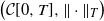 $\big(\mathcal C[0,T],\|\cdot\|_T\big)$
with respect to the speed function
 $\lambda(n)$
if the following two conditions hold:
-
(i) Condition for increments: there exist positive constants
$n_0$
,
$\alpha$
,
$\theta$
,
$\kappa$
, and c such that, for all
$n>n_0$
and all
$t,s\in[0,T]$
with
$t\neq s$
, (62)
\begin{equation} \mathbb E\bigg[\exp\!\bigg(\theta\lambda(n)\frac{|Z_n(t)-Z_n(s)|}{|t-s|^{\alpha}}\bigg)\bigg] \leq c\kappa^{\lambda(n)}. \end{equation}
-
(ii) Condition at
$t=0$
: (63)
\begin{equation} \lim_{R\rightarrow\infty}\limsup_{n\rightarrow\infty}\frac1{\lambda(n)}\log\mathbb P\big(|Z_n(0)|>R\big) = -\infty. \end{equation}


This theorem is due to Schied [Reference Schied44, Theorem 3]; see also [Reference Schied45, Corollary 7.1] or [Reference Macci and Pacchiarotti32, Theorem 1.1]. Here, we provide a proof using the Garsia–Rodemich–Rumsey inequality, as [Reference Schied44] may not be readily accessible to all readers.
First, we recall the Garsia–Rodemich–Rumsey inequality (see, e.g., [Reference Garsia, Rodemich and Rumsey19, Lemma 1.1] or [Reference Walsh48, Theorem 1.1]). Let
 $\Psi\colon[0,\infty)\to[0,\infty)$
be a non-decreasing function with
 $\lim_{x\rightarrow\infty}\Psi(x)=\infty$
, and let
 $p\colon[0,1]\rightarrow[0,1]$
be continuous and non-decreasing with
 $p(0)=0$
. For
 $u\geq\Psi(0)$
, define
 $\Psi^{-1}(u)=\sup\{v\colon\Psi(v)\leq u\}$
.
Lemma 7 ([Reference Garsia, Rodemich and Rumsey19, Lemma 1.1].) Suppose that f(s) is a continuous function on [0,Reference Anugu and Pang1], and that
 \begin{equation*} \int_0^1\int_0^1\Psi\bigg(\frac{f(s)-f(t)}{p(s-t)}\bigg)\,{\mathrm{d}} s\,{\mathrm{d}} t \leq B < \infty. \end{equation*}
Then, for any
 $s,t\in[0,1]$
,
 \begin{equation*} |f(s)-f(t)| \le 8\int_0^{|s-t|}\Psi^{-1}\bigg(\frac{4B}{u^2}\bigg)\,{\mathrm{d}} p(u). \end{equation*}
Proof of Theorem 4. Without loss of generality, we assume
 $T=1$
. For any
 $n\geq1$
and
 $r\geq 0$
, define
 $\Psi(r) \,:\!= \exp\!(\theta\lambda(n)r)$
,
 $f(r) \,:\!= Z_n(r)$
, and
 $p(r) \,:\!= r^{\alpha}$
, and let
 $$ B \,:\!= \int_0^1\int_0^1\exp\!\bigg(\frac{\theta\lambda(n)|Z_n(t)-Z_n(s)|}{|t-s|^{\alpha}}\bigg)\,{\mathrm{d}} s\,{\mathrm{d}} t. $$
By Fubini’s theorem and (62), we have
 \begin{equation} \mathbb E[B] = \int_0^1\int_0^1\mathbb E\bigg[ \exp\!\bigg(\theta\lambda(n)\frac{|Z_n(t)-Z_n(s)|}{|t-s|^{\alpha}}\bigg)\bigg]\,{\mathrm{d}} s\,{\mathrm{d}} t \leq c \kappa^{\lambda(n)}. \end{equation}
Using Lemma 7 we obtain, for any
 $\epsilon\in(0,\alpha)$
,
 \begin{align*} |Z_n(t)-Z_n(s)| & \leq \frac{8}{\theta\lambda(n)}\int_0^{|s-t|}[\log(4B)-2\log u]\,{\mathrm{d}} u^{\alpha} \\ & = \frac{8}{\theta\lambda(n)}\bigg(\log(4B)\cdot|s-t|^{\alpha}-2\alpha\int_0^{|s-t|}\log u \cdot u^{\epsilon} \cdot u^{\alpha-1-\epsilon}\,{\mathrm{d}} u\bigg) \\ & \le \frac{8}{\theta\lambda(n)}\bigg(\log(4B)\cdot|s-t|^{\alpha} + \frac{2\alpha}{{\mathrm{e}}\epsilon}\int_0^{|s-t|}u^{\alpha-1-\epsilon}\,{\mathrm{d}} u\bigg) \\ & = \frac{8}{\theta\lambda(n)}\bigg(\log(4B)\cdot|s-t|^{\alpha} + \frac{2\alpha}{{\mathrm{e}}\epsilon(\alpha-\epsilon)}|s-t|^{\alpha-\epsilon}\bigg), \end{align*}
where in the second-last step we used the inequality
 $u^{\epsilon}\log u \geq -1/({\mathrm{e}}\epsilon )$
for any
 $u\in [0,1]$
,
 $\epsilon\in(0,\alpha)$
. Hence,
 \begin{equation*} \|Z_n\|_{\alpha-\epsilon} \,:\!= {\sup}_{s,t\in[0,1],s\neq t}\frac{|Z_n(t)-Z_n(s)|}{|t-s|^{\alpha-\epsilon}} \leq \frac{8}{\theta\lambda(n)}\bigg(\log(4B) + \frac{2\alpha}{{\mathrm{e}}\epsilon(\alpha-\epsilon)}\bigg). \end{equation*}
From this and (64) we obtain
 \begin{align} \mathbb E\bigg[\exp\!\bigg(\frac{\theta\lambda(n)\|Z_n\|_{\alpha-\epsilon}}{8}\bigg)\bigg] & \leq \mathbb E\bigg[\exp\!\bigg(\log(4B) + \frac{2\alpha}{{\mathrm{e}}\epsilon(\alpha-\epsilon)}\bigg)\bigg] \nonumber \\ & = 4\exp\!\bigg(\frac{2\alpha}{{\mathrm{e}}\epsilon(\alpha-\epsilon)}\bigg)\mathbb E[B] \leq 4c\exp\!\bigg(\frac{2\alpha}{{\mathrm{e}}\epsilon(\alpha-\epsilon)}\bigg)\kappa^{\lambda(n)}. \end{align}
For any
 $R>0$
, define
 $\Gamma_R \,:\!= \big\{\xi\in\mathcal C[0,1]\colon|\xi(0)|\leq R \text{ and }\|\xi\|_{\alpha-\epsilon} \leq R\big\}$
. Then, by the Arzelà–Ascoli theorem,
 $\Gamma_R$
is compact in
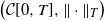 $\big(\mathcal C[0,T],\|\cdot\|_T\big)$
. Using (63), (65), and Chebyshev’s inequality, we obtain
 \begin{equation*} \lim_{R\rightarrow\infty}\lim_{n\rightarrow\infty}\frac{1}{\lambda(n)}\log\mathbb P\big(Z_n\notin\Gamma_R\big) = -\infty, \end{equation*}
which completes the proof.
The following lemma is proved in the same manner as [Reference Chang, Yao and Zajic10, Lemma 3.3].
Lemma 8.
-
(i) For any
$g\in L^{2}((\!-\infty,1])$
such that
$G^2=\int_{a}^b g^2(t)\,{\mathrm{d}} t>0$
for any
$-\infty\le a < b \le 1$
, the unique optimal solution to the minimization problem for some
$$ \min_{f\in L^2((\!-\infty, 1])}\int_{a}^b{f}^2(t)\,{\mathrm{d}} t \quad \text{subject to } \int_{a}^bg(t)f(t)\,{\mathrm{d}} t > c $$
$c\ge 0$
is
$f^*(t)=({c}/{G^2})g(t)$
for
$t\in(\!-\infty,1]$
, and the corresponding minimum is
${c^2}/{G^2}$
.
-
(ii) For any
$g_1,g_2\in L^{2}((\!-\infty,1])$
such that
$G_1^2\,:\!=\int_{a}^{b_1}g_1^2(t)\,{\mathrm{d}} t>0$
and
$G_2^2 \,:\!= \int_{b_1}^{b}g_2^2(t)\,{\mathrm{d}} t > 0$
for some
$-\infty\le a < b_1 < b\le 1$
, the unique optimal solution to the minimization problem for some
$$ \min_{f\in L^2((\!-\infty,1])}\int_{a}^b{f}^2(t)\,{\mathrm{d}} t \quad \text{subject to } \int_{a}^{b_1}g_1(t)f(t)\,{\mathrm{d}} t + \int_{b_1}^bg_2(t)f(t)\,{\mathrm{d}} t > c $$
$c\ge 0$
is given by and the corresponding minimum is
\begin{equation*} f^*(t) = \left\{ \begin{array}{l@{\quad}l} \dfrac{c}{G_1^2+G_2^2}g_1(t) \quad & if \ t \in (a, b_1], \\ \dfrac{c}{G_1^2+G_2^2}g_2(t) \quad & if \ t \in (b_1, b], \end{array} \right. \end{equation*}
${c^2}/({G_1^2+G_2^2})$
.














Acknowledgements
The authors are grateful to the anonymous referees for their valuable comments and corrections which have led to significant improvements in this paper. Part of the research was conducted during R. Wang’s visit to Michigan State University (MSU). He thanks the Department of Statistics and Probability at MSU for their warm hospitality.
Funding information
The research of R. Wang is partially supported by the NSF of Hubei Province (Grant No. 2024AFB683). The research of Y. Xiao is partially supported by the NSF grant DMS-2153846. Q. Yang is supported by National Natural Science Foundation of China (Grant Nos. 11401090, 11971097, 11971098).
Competing interests
There were no competing interests to declare during the preparation or publication of this article.


