A QUANTITATIVE DYNAMICAL BOREL–CANTELLI LEMMA FOR TWISTED RECURRENCE ON

JIACHANG LI; CHAO MA; BO WANG

doi:10.1017/S0004972726101385

A QUANTITATIVE DYNAMICAL BOREL–CANTELLI LEMMA FOR TWISTED RECURRENCE ON $[0,1]^d$

Part of: Dynamical systems with hyperbolic behavior Ergodic theory

Published online by Cambridge University Press: 22 July 2026

and

JIACHANG LI: Affiliation:
Faculty of Innovation Engineering, Macau University of Science and Technology , Macau, 999078, PR China e-mail: 3220001944@student.must.edu.mo
CHAO MA*: Affiliation:
Faculty of Innovation Engineering, Macau University of Science and Technology , Macau, 999078, PR China MUST Science and Technology Research Institute , Zhuhai, 519000, PR China
BO WANG: Affiliation:
School of Mathematics, Jiaying University , Meizhou, 514015, PR China School of Mathematics, Sun Yat-sen University, Guangzhou, 510275, PR China e-mail: math_bocomeon@163.com
*: e-mail: cma@must.edu.mo; 12490053@qq.com

Article contents

Abstract
Introduction
Proof of Theorem
Footnotes
References

Rights & Permissions

Abstract

Let $T:[0,1]^d \rightarrow [0,1]^d$ be a piecewise expanding linear map such that each domain of linearity is a coordinate-parallel hyperrectangle that T sends to $[0,1]^d$. Let $\{\mathbf {r}_n\}$ be a sequence of vectors with $\mathbf {r}_n=(r_{n, 1}, \ldots , r_{n, d}) \in (\mathbb {R}_{\geq 0})^d$. Let $m_d$ denote d-dimensional Lebesgue measure. Let $\{f_n\}$ be a sequence of piecewise Lipschitz coordinate-wise vector functions on $[0,1]^d$ with a uniform Lipschitz constant. For any given $\epsilon> 0$, we obtain a unified counting function for the shrinking target and recurrence problems:

$$ \begin{align*}\sum_{n=1}^N \mathbb{1}_{R(f_n(\mathbf{x}), \mathbf{r}_n)}(T^n \mathbf{x})=\Psi(N)+O(\Psi^{1 / 2}(N)(\log \Psi(N))^{3 / 2+\varepsilon})\end{align*} $$

for $m_d$-almost every $\mathbf {x} \in [0,1]^d$ and for all $N\in \mathbb N$, where $\Psi (N):=2^d \sum _{n=1}^N r_{n, 1} \cdots r_{n, d}$ and $R(f_n(\mathbf {x}), \mathbf {r}_n)$ is a coordinate-parallel hyperrectangle centred at $f_n(\mathbf {x})$. Our result gives a unified statement to show that the quantitative dynamical Borel–Cantelli lemma can govern both the shrinking target and recurrence problems, thereby eliminating the need for separate treatments and different proofs. This result can also apply to the situation where both problems are present simultaneously along different directions in $[0,1]^d$.

Keywords

quantitative dynamical Borel–Cantelli lemma piecewise expanding linear maps recurrence problem shrinking target problem

MSC classification

Primary: 37A05: Measure-preserving transformations

Secondary: 37D20: Uniformly hyperbolic systems (expanding, Anosov, Axiom A, etc.)

Information

Type: Research Article
Information: Bulletin of the Australian Mathematical Society , First View , pp. 1 - 12

DOI: https://doi.org/10.1017/S0004972726101385 [Opens in a new window]
Copyright: © The Author(s), 2026. Published by Cambridge University Press on behalf of Australian Mathematical Publishing Association Inc.

1 Introduction

Let $(X, \mathcal {B}, \mu , T)$ be a measure-preserving dynamical system with a compatible metric $\rho $ , that is, $(X, \rho )$ is a metric space, $\mathcal {B}$ is a Borel $\sigma $ -algebra of X and $\mu $ is a T-invariant probability measure. Suppose that $(X, \rho )$ is complete and separable. Poincaré’s recurrence theorem, one of the most fundamental results in dynamical systems and ergodic theory (see [Reference Einsiedler and Ward3, Theorem 2.11]), states that $\mu $ -almost every point returns close to itself under a measure-preserving map T, that is,

$$ \begin{align*} \liminf _{n \rightarrow \infty} \rho(T^n x, x)=0. \end{align*} $$

Boshernitzan proved the first general quantitative recurrence result in [Reference Boshernitzan2, Theorem 1.2]. Specifically, assume that the $\alpha $ -dimensional Hausdorff measure of X is $\sigma $ -finite for some $\alpha>0$ . Then,

$$ \begin{align*} \liminf _{n \rightarrow \infty} n^{1 / \alpha} \rho(T^n x, x)<\infty \quad \text {for } \mu \text {-a.e. } x \in X. \end{align*} $$

Here, $\mu $ -a.e. denotes ‘almost every’ with respect to $\mu $ . Put differently, for $\mu $ -a.e. $x \in X$ , there is a constant $c(x)>0$ such that $\rho (T^n x, x)<c(x) n^{-1 / \alpha }$ for infinitely many $n \in \mathbb {N}$ . This result motivates the study of the size of the set

$$ \begin{align*} \mathcal{R}(\psi):=\{x \in X: \rho(T^n x, x)<\psi(n) \text { for i.m. } n \in \mathbb{N}\}. \end{align*} $$

Here, $\psi : \mathbb {N} \rightarrow \mathbb {R}^{+}$ is a positive function and i.m. denotes ‘infinitely many’. The zero-full law for the $\mu $ -measure of the recurrence set $\mathcal {R}(\psi )$ , often referred to as the quantitative recurrence property or dynamical Borel–Cantelli lemma for recurrence theory, has been extensively studied in various dynamical systems (see, for example, [Reference He, Li and Velani4–Reference Hussain, Li, Simmons and Wang6]). In other words, Boshernitzan’s result states ${\sum _{n=1}^{\infty } \mathbb {1}_{B(x, c(x) n^{-1 / \alpha })}(T^n x)=\infty }$ for $\mu $ -a.e. $x \in X$ , where $\mathbb {1}_{B(x, c(x) n^{-1 / \alpha })}$ denotes the characteristic function of the open ball ${B(x, c(x) n^{-1 / \alpha })}$ with centre $x \in X$ and radius $c(x) n^{-1 / \alpha }$ . This result motivates us to study a significantly stronger quantitative statement for the counting function

$$ \begin{align*}\sum_{n=1}^N \mathbb{1}_{B(x, \psi(n))}(T^n x) :=\#\{1 \leq n \leq N: T^n x \in B(x, \psi(n))\},\end{align*} $$

where $N\in \mathbb N$ , often referred to as the quantitative dynamical Borel–Cantelli lemma (for related results, see [Reference He, Li and Velani4, Reference Levesley, Li, Simmons and Velani8, Reference Li, Liao, Velani and Zorin9]). Of particular relevance to our work is the recent study by Levesley et al. [Reference Levesley, Li, Simmons and Velani8], which gives the recurrence counting function for piecewise expanding linear maps on $[0,1]^d$ , and clarifies the distinct proofs for the recurrence counting function and the shrinking target problem introduced as follows.

The shrinking target problem involves determining the rate at which the orbit of a $\mu $ -typical point accumulates near a given point $y \in X$ . More specifically, for $\psi : \mathbb {N} \rightarrow ~ \mathbb {R}^{+}$ , define

$$ \begin{align*} \mathcal{R}^y(\psi):=\{x \in X: \rho(T^n x, y)<\psi(n) \text { for i.m. } n \in \mathbb{N}\}. \end{align*} $$

In [Reference Li, Liao, Velani and Zorin9], Li et al. prove that the results for the counting function hold for a large class of measure-preserving dynamical systems and the ‘target’ sets can be any measurable subset centred at a given point of X.

These two problems are among the most commonly studied, but they are typically treated separately using different methods, as in [Reference He, Li and Velani4, Reference Levesley, Li, Simmons and Velani8]. A more general definition, known as the twisted recurrence or modified shrinking target problem, unifies the two problems. Specifically, for $\psi : \mathbb {N} \rightarrow \mathbb {R}^{+}$ and a sequence $\{f_n\}$ of Borel measurable functions on X, define

$$ \begin{align*} \mathcal{R}^f(\psi):=\{x \in X: \rho(T^n x, f_n(x))<\psi(n) \text { for i.m. } n \in \mathbb{N}\}. \end{align*} $$

It follows that if $f_1=f_2=\cdots =f_n=\cdots =\mathrm {Id}_X$ , then $ \mathcal {R}^f(\psi )=\mathcal {R}(\psi )$ . Moreover, if ${f_1=f_2=\cdots =f_n=\cdots \equiv y}$ , then $ \mathcal {R}^f(\psi )=\mathcal {R}^y(\psi )$ . The zero-full law for the $\mu $ -measure of the twisted recurrence set has been the subject of significant study in various dynamical systems (see [Reference Kleinbock and Zheng7, Reference Li and Ma10, Reference Shen11, Reference Wu14]). For Hausdorff dimension results, see [Reference Shen11–Reference Yuan and Wang16]. However, the quantitative dynamical Borel–Cantelli lemma has not yet been established for twisted recurrences.

Following the same setup and similar methods as in [Reference Levesley, Li, Simmons and Velani8], our goal in this paper is to establish, via a unified proof, the counting function for both the shrinking target and recurrence problems. Throughout the paper, we take X to be the unit hypercube $[0,1]^d$ endowed with a metric $\rho $ . Let $m_d$ denote the d-dimensional Lebesgue measure. Let $\mathcal {P}_m$ denote the collection of cylinder sets $J_m$ of order m that partition $[0,1]^d$ . Let $D_x T$ denote the derivative of T at $x \in X$ .

The following definition introduces the class of measure-preserving systems $([0,1]^d, T, m_d)$ , as defined in [Reference Levesley, Li, Simmons and Velani8].

Definition 1.1 (Piecewise expanding linear map [Reference Levesley, Li, Simmons and Velani8])

We say that $T:[0,1]^d \rightarrow [0,1]^d$ is a piecewise expanding linear map if each domain of linearity $J_1$ is a coordinate-parallel hyperrectangle that T sends to $[0,1]^d$ such that $D_{\mathbf {x}} T|_{J_1}$ is a diagonal matrix and the following conditions hold.

(i) For general $m \in \mathbb {N}$ , $J_m=\prod _{i=1}^d J_m^{(i)} \in \mathcal {P}_m$ is the coordinate-parallel hyperrectangle of linearity for $T^m$ such that $D_{\mathbf {x}} T$ is the same for any $\mathbf {x} \in J_m$ , so we simply write $T^{\prime }|_{J_m}$ . For $1 \leq i \leq d$ , let $K_{J_m}^{(i)}$ be the $(i, i)$ th component of the diagonal matrix $(T^m)^{\prime }|_{J_m}$ and $K_{J_m}:=\prod _{i=1}^d K_{J_m}^{(i)}$ so that $T^m|_{J_m}$ is a similarity with the dilatation factor $|K_{J_m}|$ .
(ii) T is expanding in all directions, that is, there exists a constant $\lambda>1$ such that for $1 \leq i \leq d$ , $m \in \mathbb {N}$ and $J_m \in \mathcal {P}_m$ ,
(1.1) $$ \begin{align} |K_{J_m}^{(i)}| \geq \lambda^m. \end{align} $$
(iii) T is a measure-preserving transformation with respect to $m_d$ , that is, $m_d$ is a T-invariant probability measure. For any measurable set $F \subseteq J_m$ , due to linearity,
$$ \begin{align*} m_d(T^m F)=|K_{J_m}| m_d(F). \end{align*} $$
(iv) [Reference Levesley, Li, Simmons and Velani8, Proposition 4.1]. T is hyperrectangular exponentially mixing with respect to $m_d$ , that is, there is a constant $\gamma $ with $0<\gamma <1$ such that for any ${n \in \mathbb {N}}$ , any coordinate-parallel hyperrectangle $R \subset [0,1]^d$ and any measurable set $F \subset ~ [0,1]^d$ ,
$$ \begin{align*} m_d(R \cap T^{-n}F)=m_d(R) m_d(F)+O(\gamma^n) m_d(F). \end{align*} $$

Remark 1.2. Given the set up as above, for $1 \leq i \leq d$ and any $\mathbf {x}, \mathbf {y} \in J_m$ with $x_i \neq y_i$ ,

$$ \begin{align*}|K_{J_m}^{(i)}|=\frac{1}{m_1(J_m^{(i)})}=\frac{\rho((T^m \mathbf{x})_i,(T^m \mathbf{y})_i)}{\rho(x_i, y_i)}\end{align*} $$

so that $|K_{J_m}|=1 / m_d(J_m)$ . As a result, $\sum _{J_m \in \mathcal {P}_m}|K_{J_m}|^{-1}=1$ . From [Reference Levesley, Li, Simmons and Velani8, Proposition 4.1], we can take $\gamma :=1 / \lambda $ and rewrite (1.1) as

$$ \begin{align*} |K_{J_m}^{(i)}| \geq \gamma^{-m} \quad(1 \leq i \leq d). \end{align*} $$

Well-known dynamical systems that satisfy the conditions of Definition 1.1 include the tent map, the Lüroth map and expanding, diagonal integer matrix transformations of the d-dimensional torus $\mathbb {T}^d$ .

Next, we specify the class of functions f that can be treated by our technique.

Definition 1.3 (Piecewise Lipschitz coordinate-wise vector function)

Let $p>0$ . We say that $f:[0,1]^d \rightarrow [0,1]^d$ is a Lipschitz coordinate-wise vector function, if for ${1 \leq i \leq d}$ and any $\mathbf {x}, \mathbf {y} \in [0,1]^d$ ,

$$ \begin{align*}f(\mathbf{x})=(f_1(x_1), f_2(x_2), \ldots, f_d(x_d)) \quad\text{and}\quad \rho (f_i(x_i),f_i(y_i)) \leq p\rho (x_i,y_i). \end{align*} $$

Furthermore, f is piecewise Lipschitz if there exist finitely many measurable subsets $U_j$ in $[0,1]^d$ such that $m_d([0,1]^d \backslash \bigcup _{j}U_j )=0$ and $f|_{U_j}: U_j \rightarrow [0,1]^d$ is a Lipschitz function for each j.

For example, when $d=1$ , the function $f(x)=2x \bmod 1$ is piecewise Lipschitz but not Lipschitz on $[0,1)$ .

Motivated by the weighted theory of Diophantine approximation, for a sequence of piecewise Lipschitz coordinate-wise vector functions $\{f_n:[0,1]^d \rightarrow [0,1]^d\}$ with a uniform Lipschitz constant p and a sequence $\{\mathbf {r}_n\}$ of vectors with $\mathbf {r}_n=(r_{n, 1}, \ldots , r_{n, d}) \in (\mathbb {R}_{\geq 0})^d$ , define

$$ \begin{align*} \mathcal{R}^f(\{\mathbf{r}_n\})& :=\{\mathbf{x} \in[0,1]^d: T^n \mathbf{x} \in R(f_n(\mathbf{x}), \mathbf{r}_n) \text { for i.m. } n \in \mathbb{N}\} \\ &\; =\bigg\{\mathbf{x} \in[0,1]^d: T^n \mathbf{x} \in \prod_{i=1}^d B(f_n^{(i)}(x_i), r_{n, i})\text { for i.m. } n \in \mathbb{N}\bigg\} \\ &\; =\{\mathbf{x} \in[0,1]^d: \rho((T^n \mathbf{x})_i, f_n^{(i)}(x_i)) \leq r_{n, i} \text{ for }1 \leq i \leq d \text { and i.m. } n \in \mathbb{N} \}, \end{align*} $$

StartLayout 1st Row 1st Column script upper R Superscript f Baseline left parenthesis StartSet bold r Subscript n Baseline EndSet right parenthesis 2nd Column colon equals StartSet bold x element of left bracket 0 comma 1 right bracket Superscript d Baseline colon upper T Superscript n Baseline bold x element of upper R left parenthesis f Subscript n Baseline left parenthesis bold x right parenthesis comma bold r Subscript n Baseline right parenthesis for i period m period n element of double struck upper N EndSet 2nd Row 1st Column Blank 2nd Column equals StartSet bold x element of left bracket 0 comma 1 right bracket Superscript d Baseline colon upper T Superscript n Baseline bold x element of product Underscript i equals 1 Overscript d Endscripts upper B left parenthesis f Subscript n Superscript left parenthesis i right parenthesis Baseline left parenthesis x Subscript i Baseline right parenthesis comma r Subscript n comma i Baseline right parenthesis for i period m period n element of double struck upper N EndSet 3rd Row 1st Column Blank 2nd Column equals StartSet bold x element of left bracket 0 comma 1 right bracket Superscript d Baseline colon rho left parenthesis left parenthesis upper T Superscript n Baseline bold x right parenthesis Subscript i Baseline comma f Subscript n Superscript left parenthesis i right parenthesis Baseline left parenthesis x Subscript i Baseline right parenthesis right parenthesis less than or equals r Subscript n comma i Baseline for 1 less than or equals i less than or equals d and i period m period n element of double struck upper N EndSet comma EndLayout

and similarly for $N\in \mathbb N$ , define

$$ \begin{align*}\sum_{n=1}^N \mathbb{1}_{R(f_n(\mathbf{x}), \mathbf{r}_n)}(T^n \mathbf{x}):=\#\{1 \leq n \leq N: T^n \mathbf{x} \in R(f_n(\mathbf{x}), \mathbf{r}_n)\}.\end{align*} $$

We now proceed to our main theorem.

Theorem 1.4. Let $T:[0,1]^d \rightarrow [0,1]^d$ be a piecewise expanding linear map. Let $\{f_n\}$ be a sequence of piecewise Lipschitz coordinate-wise vector functions on $[0,1]^d$ with a uniform Lipschitz constant p. For any sequence of vectors $\{\mathbf {r}_n\}$ in $(\mathbb {R}_{\geq 0})^d $ and any given $\varepsilon>0$ ,

$$ \begin{align*} \sum_{n=1}^N \mathbb{1}_{R(f_n(\mathbf{x}), \mathbf{r}_n)}(T^n \mathbf{x})=\Psi(N)+O(\Psi^{1 / 2}(N)(\log \Psi(N))^{3 / 2+\varepsilon}) \end{align*} $$

for $m_d$ -a.e. $\mathbf {x} \in [0,1]^d$ , where $\Psi (N):=2^d \sum _{n=1}^N r_{n, 1} \cdots r_{n, d}$ . In particular,

$$ \begin{align*} m_d(\mathcal{R}^f(\{\mathbf{r}_n\}))= \begin{cases}0 & \text {if } \sum_{n=1}^{\infty} r_{n, 1} \cdots r_{n, d}<\infty, \\ 1 & \text {if } \sum_{n=1}^{\infty} r_{n, 1} \cdots r_{n, d}=\infty .\end{cases} \end{align*} $$

m Subscript d Baseline left parenthesis script upper R Superscript f Baseline left parenthesis StartSet bold r Subscript n Baseline EndSet right parenthesis right parenthesis equals StartLayout Enlarged left brace 1st Row 1st Column 0 2nd Column if sigma summation Underscript n equals 1 Overscript infinity Endscripts r Subscript n comma 1 Baseline midline horizontal ellipsis r Subscript n comma d Baseline less than infinity comma 2nd Row 1st Column 1 2nd Column if sigma summation Underscript n equals 1 Overscript infinity Endscripts r Subscript n comma 1 Baseline midline horizontal ellipsis r Subscript n comma d Baseline equals infinity period EndLayout

2 Proof of Theorem 1.4

For a sequence of piecewise Lipschitz coordinate-wise vector functions $\{f_n\}$ on $[0,1]^d$ with a uniform Lipschitz constant p and a sequence $\{\mathbf {r}_n\}$ of vectors with $\mathbf {r}_n=(r_{n, 1}, \ldots , r_{n, d}) \in (\mathbb {R}_{\geq 0})^d$ , define

$$ \begin{align*} A_n:=\{\mathbf{x} \in[0,1]^d: T^n \mathbf{x} \in R(f_n(\mathbf{x}), \mathbf{r}_n) \}. \end{align*} $$

Unlike the shrinking target case, the sets $A_n$ cannot be expressed in the form $T^{-n} R_n$ for some hyperrectangles $R_n$ . To address this, we follow the approach from [Reference Li and Ma10, Lemma 3.2], which considers $A_n$ locally by studying its intersection with

$$ \begin{align*} A_n \cap f_n^{-1} R(f_n(\mathbf{x}), p\mathbf{r}), \end{align*} $$

where $\mathbf {r}=(r_1, \ldots , r_d) \in (\mathbb {R}_{\geq 0})^d$ . This intersection can be approximated by the preimages of hyperrectangles under T.

Lemma 2.1 [Reference Li and Ma10, Lemma 3.2]

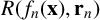
Let $R(f_n(\mathbf {x}), p \mathbf {r})$ be a coordinate-parallel hyperrectangle centred at $f_n(\mathbf {x}) \in [0,1]^d$ , where $p\mathbf {r}=(pr_1, \ldots , pr_d) \in (\mathbb {R}_{\geq 0})^d$ . For any $n \in \mathbb {N}$ and any subset S of $f_n^{-1} R(f_n(\mathbf {x}), p\mathbf {r})$ , we have

$$ \begin{align*} S \cap A_n \subset S \cap T^{-n} R(f_n(\mathbf{x}), \mathbf{r}_n+p \mathbf{r}). \end{align*} $$

Furthermore, if $pr_i \leq r_{n, i}$ for $1 \leq i \leq d$ , then

$$ \begin{align*} S \cap T^{-n} R(f_n(\mathbf{x}), \mathbf{r}_n-p \mathbf{r}) \subset S \cap A_n. \end{align*} $$

The following result [Reference Beresnevich, Ramírez, Velani, Badziahin, Gorodnik and Peyerimhoff1, Lemma 1.5] serves as a key tool in metric Diophantine approximation for proving counting statements.

Lemma 2.2 [Reference Beresnevich, Ramírez, Velani, Badziahin, Gorodnik and Peyerimhoff1, Lemma 1.5]

Let $(X, \mathcal {B}, \mu )$ be a probability space, let $(f_n(x))_{n \in \mathbb {N}}$ be a sequence of nonnegative $\mu $ -measurable functions defined on X and let $(c_n)_{n \in \mathbb {N}},(\phi _n)_{n \in \mathbb {N}}$ be sequences of real numbers such that $ 0 \leq c_n \leq \phi _n \ (n=1,2, \ldots ). $ Suppose that for arbitrary $a, b \in \mathbb {N}$ with $a<b$ ,

(2.1) $$ \begin{align} \int_X\bigg(\sum_{n=a}^b(f_n(x)-c_n)\bigg)^2 \,{d} \mu(x) \leq C \sum_{n=a}^b \phi_n \end{align} $$

for an absolute constant $C>0$ . Then, for any given $\varepsilon>0$ ,

$$ \begin{align*} \sum_{n=1}^N f_n(x)=\sum_{n=1}^N c_n+O\Big(\Phi(N)^{1 / 2} \log ^{{3}/{2}+\varepsilon} \Phi(N)+\max _{1 \leq k \leq N} c_k\Big) \end{align*} $$

for $\mu $ -a.e. $x \in X$ , where $\Phi (N):=\sum _{n=1}^N \phi _n$ .

To establish our result, we apply Lemma 2.2 with

$$ \begin{align*} X:=[0,1]^d, \quad f_n(x):=\mathbb{1}_{A_n}(\mathbf{x}) \quad \text { and } \quad c_n:=\phi_n:=m_d(A_n), \end{align*} $$

so that $\Phi (N):=\sum _{n=1}^N m_d(A_n)$ . For any $a, b \in \mathbb {N}$ with $a<b$ ,

$$ \begin{align*} & \bigg(\sum_{n=a}^b(f_n(x)-c_n)\bigg)^2=\bigg(\sum_{n=a}^b(\mathbb{1}_{A_n}(\mathbf{x})-m_d(A_n))\bigg)^2 \\ &\quad=\bigg(\sum_{n=a}^b \mathbb{1}_{A_n}(\mathbf{x})\bigg)^2+\bigg(\sum_{n=a}^b m_d(A_n)\bigg)^2-2 \sum_{n=a}^b \mathbb{1}_{A_n}(\mathbf{x}) \cdot \sum_{n=a}^b m_d(A_n) \\ &\quad =\sum_{n=a}^b \mathbb{1}_{A_n}(\mathbf{x})+2\mathop{\sum\sum}_{a\leq m<n\leq b} \mathbb{1}_{A_m}(\mathbf{x}) \mathbb{1}_{A_n}(\mathbf{x})+\bigg(\sum_{n=a}^b m_d(A_n)\bigg)^2-2 \sum_{n=a}^b m_d(A_n) \cdot \sum_{n=a}^b \mathbb{1}_{A_n}(\mathbf{x}), \end{align*} $$

StartLayout 1st Row 1st Column Blank 2nd Column left parenthesis sigma summation Underscript n equals a Overscript b Endscripts left parenthesis f Subscript n Baseline left parenthesis x right parenthesis minus c Subscript n Baseline right parenthesis right parenthesis squared equals left parenthesis sigma summation Underscript n equals a Overscript b Endscripts left parenthesis double struck 1 Subscript upper A Sub Subscript n Subscript Baseline left parenthesis bold x right parenthesis minus m Subscript d Baseline left parenthesis upper A Subscript n Baseline right parenthesis right parenthesis right parenthesis squared 2nd Row 1st Column Blank 2nd Column equals left parenthesis sigma summation Underscript n equals a Overscript b Endscripts double struck 1 Subscript upper A Sub Subscript n Subscript Baseline left parenthesis bold x right parenthesis right parenthesis squared plus left parenthesis sigma summation Underscript n equals a Overscript b Endscripts m Subscript d Baseline left parenthesis upper A Subscript n Baseline right parenthesis right parenthesis squared minus 2 sigma summation Underscript n equals a Overscript b Endscripts double struck 1 Subscript upper A Sub Subscript n Baseline left parenthesis bold x right parenthesis dot sigma summation Underscript n equals a Overscript b Endscripts m Subscript d Baseline left parenthesis upper A Subscript n Baseline right parenthesis 3rd Row 1st Column Blank 2nd Column equals sigma summation Underscript n equals a Overscript b Endscripts double struck 1 Subscript upper A Sub Subscript n Subscript Baseline left parenthesis bold x right parenthesis plus 2 sigma summation sigma summation Underscript a less than or equals m less than n less than or equals b Endscripts double struck 1 Subscript upper A Sub Subscript m Subscript Baseline left parenthesis bold x right parenthesis double struck 1 Subscript upper A Sub Subscript n Subscript Baseline left parenthesis bold x right parenthesis plus left parenthesis sigma summation Underscript n equals a Overscript b Endscripts m Subscript d Baseline left parenthesis upper A Subscript n Baseline right parenthesis right parenthesis squared minus 2 sigma summation Underscript n equals a Overscript b Endscripts m Subscript d Baseline left parenthesis upper A Subscript n Baseline right parenthesis dot sigma summation Underscript n equals a Overscript b Endscripts double struck 1 Subscript upper A Sub Subscript n Subscript Baseline left parenthesis bold x right parenthesis comma EndLayout

so the left-hand side of (2.1) is equal to

(2.2) $$ \begin{align} \sum_{n=a}^b m_d(A_n)+2\mathop{\sum\sum}_{a\leq m<n\leq b} m_d(A_m \cap A_n)-\bigg(\sum_{n=a}^b m_d(A_n)\bigg)^2. \end{align} $$

2.1 Calculating the measure of $A_n$

In this section, we aim to obtain the relationship between $\Phi (N)$ and $\Psi (N)$ , thereby connecting the above lemma with our result.

Proposition 2.3. For arbitrary $N \in \mathbb {N}$ ,

$$ \begin{align*} \Phi(N)=\sum_{n=1}^N m_d(A_n)=2^d \sum_{n=1}^N r_{n, 1} \cdots r_{n, d}+O(1)= \Psi(N)+O(1). \end{align*} $$

Proof. Consider a sequence of real numbers $\{\varepsilon _n\}_{n \in \mathbb {N}}$ such that $\varepsilon _n \in (0,1 / p)$ for all $n \in \mathbb {N}$ and $\lim _{n \rightarrow \infty } \varepsilon _n=0$ , where p is the Lipschitz constant in Definition 1.3. For sufficiently large $n \in \mathbb {N}$ and $1 \leq i \leq d$ , we have $2\varepsilon _n r_{n, i}<r_{n, i}<1$ . Accordingly, for $1 \leq i \leq d$ , we partition the unit interval $[0,1]$ into $ \lceil {1}/{(2\varepsilon _n r_{n, i})}\rceil $ pairwise disjoint subintervals of equal length

(2.3) $$ \begin{align} l_{n,i}:=\frac{1}{\lceil{1}/{(2\varepsilon_n r_{n, i})}\rceil}. \end{align} $$ l Subscript n comma i Baseline colon equals StartFraction 1 Over left ceiling 1 divided by left parenthesis 2 epsilon Subscript n Baseline r Subscript n comma i Baseline right parenthesis right ceiling EndFraction period

Taking the product, we obtain a decomposition of the unit hypercube $[0,1]^d$ into

$$ \begin{align*} \mathcal{I}:=\prod_{i=1}^d\bigg\lceil\frac{1}{2\varepsilon_n r_{n, i}}\bigg\rceil \end{align*} $$ script upper I colon equals product Underscript i equals 1 Overscript d Endscripts left ceiling StartFraction 1 Over 2 epsilon Subscript n Baseline r Subscript n comma i Baseline EndFraction right ceiling

pairwise disjoint coordinate-parallel hyperrectangles

$$ \begin{align*} \{R(\mathbf{x}_j, \mathbf{t}_n): \mathbf{x}_j \in[0,1]^d\}_{j \in \mathcal{I}}, \end{align*} $$

where $\mathbf {t}_n=(t_{n,1}, \ldots , t_{n,d}):=\tfrac 12\mathbf {l}_n=(\tfrac 12l_{n,1}, \ldots ,\tfrac 12l_{n,d})$ , and the sidelength $l_{n,i}$ of each coordinate-parallel hyperrectangle in the ith direction is defined in (2.3) and satisfies $l_{n,i} \leq 2\varepsilon _n r_{n, i}$ for $1 \leq i \leq d$ .

For any $\mathbf {y} \in R(\mathbf {x}, \mathbf {t}_n)$ , we have $f_n(\mathbf {y})=(f_n^{(1)}(y_1),f_n^{(2)}(y_2),\ldots ,f_n^{(d)}(y_d))$ and $\rho (f_n^{(i)}(y_i),f_n^{(i)}(x_i)) \leq p\rho (y_i,x_i) \leq pt_{n,i}$ for $1 \leq i \leq d$ so that $\mathbf {y} \in f_n^{-1}R(f_n(\mathbf {x}), \mathbf {t}_n)$ . Consequently, for each $j \in \mathcal {I}$ , we have $R(\mathbf {x}_j, \mathbf {t}_n) \subset f_n^{-1}R(f_n(\mathbf {x}_j), p\mathbf {t}_n)$ .

Since $\varepsilon _n \in (0,1 / p)$ for all $n \in \mathbb {N}$ , we have $p\varepsilon _n r_{n, i}<r_{n, i}$ for $1 \leq i \leq d$ . By Lemma 2.1 and since $t_{n,i}=\tfrac 12l_{n,i} \leq \varepsilon _n r_{n, i}$ for $1 \leq i \leq d$ ,

$$ \begin{align*} R(\mathbf{x}_j, \mathbf{t}_n) & \cap T^{-n} R(f_n(\mathbf{x}_j),(1-p \varepsilon_n) \mathbf{r}_n) \subset R(\mathbf{x}_j, \mathbf{t}_n) \cap T^{-n} R(f_n(\mathbf{x}_j), \mathbf{r}_n-p \mathbf{t}_n) \\ & \subset R(\mathbf{x}_j, \mathbf{t}_n) \cap A_n \subset R(\mathbf{x}_j, \mathbf{t}_n) \cap T^{-n} R(f_n(\mathbf{x}_j), \mathbf{r}_n+p \mathbf{t}_n) \\ &\subset R(\mathbf{x}_j, \mathbf{t}_n) \cap T^{-n} R(f_n(\mathbf{x}_j),(1+p \varepsilon_n) \mathbf{r}_n). \end{align*} $$

StartLayout 1st Row 1st Column upper R left parenthesis bold x Subscript j Baseline comma bold t Subscript n Baseline right parenthesis 2nd Column intersection upper T Superscript negative n Baseline upper R left parenthesis f Subscript n Baseline left parenthesis bold x Subscript j Baseline right parenthesis comma left parenthesis 1 minus p epsilon Subscript n Baseline right parenthesis bold r Subscript n Baseline right parenthesis subset of upper R left parenthesis bold x Subscript j Baseline comma bold t Subscript n Baseline right parenthesis intersection upper T Superscript negative n Baseline upper R left parenthesis f Subscript n Baseline left parenthesis bold x Subscript j Baseline right parenthesis comma bold r Subscript n Baseline minus p bold t Subscript n Baseline right parenthesis 2nd Row 1st Column Blank 2nd Column subset of upper R left parenthesis bold x Subscript j Baseline comma bold t Subscript n Baseline right parenthesis intersection upper A Subscript n Baseline subset of upper R left parenthesis bold x Subscript j Baseline comma bold t Subscript n Baseline right parenthesis intersection upper T Superscript negative n Baseline upper R left parenthesis f Subscript n Baseline left parenthesis bold x Subscript j Baseline right parenthesis comma bold r Subscript n Baseline plus p bold t Subscript n Baseline right parenthesis 3rd Row 1st Column Blank 2nd Column subset of upper R left parenthesis bold x Subscript j Baseline comma bold t Subscript n Baseline right parenthesis intersection upper T Superscript negative n Baseline upper R left parenthesis f Subscript n Baseline left parenthesis bold x Subscript j Baseline right parenthesis comma left parenthesis 1 plus p epsilon Subscript n Baseline right parenthesis bold r Subscript n Baseline right parenthesis period EndLayout

By the hyperrectangular exponentially mixing property, there exists a constant $C_1>0$ such that

$$ \begin{align*} m_d & (R(\mathbf{x}_j, \mathbf{t}_n) \cap A_n) \geq m_d(R(\mathbf{x}_j, \mathbf{t}_n) \cap T^{-n} R(f_n(\mathbf{x}_j),(1-p \varepsilon_n) \mathbf{r}_n)) \\ & \geq(m_d(R(\mathbf{x}_j, \mathbf{t}_n))-C_1 \gamma^n) m_d(R(f_n(\mathbf{x}_j),(1-p \varepsilon_n) \mathbf{r}_n)) \\ & =m_d(R(\mathbf{x}_j, \mathbf{t}_n)) 2^d(1-p \varepsilon_n)^d r_{n, 1} \cdots r_{n, d}-C_1 \gamma^n 2^d(1-p \varepsilon_n)^d r_{n, 1} \cdots r_{n, d} \\ & \geq m_d(R(\mathbf{x}_j, \mathbf{t}_n)) 2^d(1-p \varepsilon_n)^d r_{n, 1} \cdots r_{n, d}-C_1 \gamma^n 2^d r_{n, 1} \cdots r_{n, d}. \end{align*} $$

StartLayout 1st Row 1st Column m Subscript d 2nd Column left parenthesis upper R left parenthesis bold x Subscript j Baseline comma bold t Subscript n Baseline right parenthesis intersection upper A Subscript n Baseline right parenthesis greater than or equals m Subscript d Baseline left parenthesis upper R left parenthesis bold x Subscript j Baseline comma bold t Subscript n Baseline right parenthesis intersection upper T Superscript negative n Baseline upper R left parenthesis f Subscript n Baseline left parenthesis bold x Subscript j Baseline right parenthesis comma left parenthesis 1 minus p epsilon Subscript n Baseline right parenthesis bold r Subscript n Baseline right parenthesis right parenthesis 2nd Row 1st Column Blank 2nd Column greater than or equals left parenthesis m Subscript d Baseline left parenthesis upper R left parenthesis bold x Subscript j Baseline comma bold t Subscript n Baseline right parenthesis right parenthesis minus upper C 1 gamma Superscript n Baseline right parenthesis m Subscript d Baseline left parenthesis upper R left parenthesis f Subscript n Baseline left parenthesis bold x Subscript j Baseline right parenthesis comma left parenthesis 1 minus p epsilon Subscript n Baseline right parenthesis bold r Subscript n Baseline right parenthesis right parenthesis 3rd Row 1st Column Blank 2nd Column equals m Subscript d Baseline left parenthesis upper R left parenthesis bold x Subscript j Baseline comma bold t Subscript n Baseline right parenthesis right parenthesis 2 Superscript d Baseline left parenthesis 1 minus p epsilon Subscript n Baseline right parenthesis Superscript d Baseline r Subscript n comma 1 Baseline midline horizontal ellipsis r Subscript n comma d Baseline minus upper C 1 gamma Superscript n Baseline 2 Superscript d Baseline left parenthesis 1 minus p epsilon Subscript n Baseline right parenthesis Superscript d Baseline r Subscript n comma 1 Baseline midline horizontal ellipsis r Subscript n comma d Baseline 4th Row 1st Column Blank 2nd Column greater than or equals m Subscript d Baseline left parenthesis upper R left parenthesis bold x Subscript j Baseline comma bold t Subscript n Baseline right parenthesis right parenthesis 2 Superscript d Baseline left parenthesis 1 minus p epsilon Subscript n Baseline right parenthesis Superscript d Baseline r Subscript n comma 1 Baseline midline horizontal ellipsis r Subscript n comma d Baseline minus upper C 1 gamma Superscript n Baseline 2 Superscript d Baseline r Subscript n comma 1 Baseline midline horizontal ellipsis r Subscript n comma d Baseline period EndLayout

Since $\lim _{n \rightarrow \infty } \varepsilon _n=0$ , for sufficiently large $n \in \mathbb {N}$ , we have $(1-p\varepsilon _n)^d \geq 1-dp\varepsilon _n$ . Together with $\# \mathcal {I} \geq {1}/{(2^d\varepsilon _n^dr_{n, 1} \cdots r_{n, d})}$ , we consequently obtain

$$ \begin{align*} m_d(A_n)&=\sum_{j \in \mathcal{I}} m_d(R(\mathbf{x}_j, \mathbf{t}_n) \cap A_n) \\ &\geq 2^d(1-p \varepsilon_n)^d r_{n, 1} \cdots r_{n, d}-\# \mathcal{I}C_1 \gamma^n 2^d r_{n, 1} \cdots r_{n, d}\\ &\geq 2^d r_{n, 1} \cdots r_{n, d}-2^{d} d p \varepsilon_n r_{n, 1} \cdots r_{n, d}- C_1 \gamma^n /{\varepsilon_n^d}. \end{align*} $$

StartLayout 1st Row 1st Column m Subscript d Baseline left parenthesis upper A Subscript n Baseline right parenthesis 2nd Column equals sigma summation Underscript j element of script upper I Endscripts m Subscript d Baseline left parenthesis upper R left parenthesis bold x Subscript j Baseline comma bold t Subscript n Baseline right parenthesis intersection upper A Subscript n Baseline right parenthesis 2nd Row 1st Column Blank 2nd Column greater than or equals 2 Superscript d Baseline left parenthesis 1 minus p epsilon Subscript n Baseline right parenthesis Superscript d Baseline r Subscript n comma 1 Baseline midline horizontal ellipsis r Subscript n comma d Baseline minus number sign script upper I upper C 1 gamma Superscript n Baseline 2 Superscript d Baseline r Subscript n comma 1 Baseline midline horizontal ellipsis r Subscript n comma d Baseline 3rd Row 1st Column Blank 2nd Column greater than or equals 2 Superscript d Baseline r Subscript n comma 1 Baseline midline horizontal ellipsis r Subscript n comma d Baseline minus 2 Superscript d Baseline d p epsilon Subscript n Baseline r Subscript n comma 1 Baseline midline horizontal ellipsis r Subscript n comma d Baseline minus upper C 1 gamma Superscript n Baseline divided by epsilon Subscript n Superscript d Baseline period EndLayout

Similarly, for the other side,

$$ \begin{align*} m_d & (R(\mathbf{x}_j, \mathbf{t}_n) \cap A_n) \leq m_d(R(\mathbf{x}_j, \mathbf{t}_n) \cap T^{-n} R(f_n(\mathbf{x}_j),(1+p \varepsilon_n) \mathbf{r}_n)) \\ & \leq(m_d(R(\mathbf{x}_j, \mathbf{t}_n))+C_1 \gamma^n) m_d(R(f_n(\mathbf{x}_j),(1+p \varepsilon_n) \mathbf{r}_n)) \\ & =m_d(R(\mathbf{x}_j, \mathbf{t}_n)) 2^d(1+p \varepsilon_n)^d r_{n, 1} \cdots r_{n, d}+C_1 \gamma^n 2^d(1+p \varepsilon_n)^d r_{n, 1} \cdots r_{n, d} \\ & \leq m_d(R(\mathbf{x}_j, \mathbf{t}_n)) 2^d(1+p \varepsilon_n)^d r_{n, 1} \cdots r_{n, d}+C_1 \gamma^n 2^{2 d} r_{n, 1} \cdots r_{n, d}. \end{align*} $$

Since $\lim _{n \rightarrow \infty } \varepsilon _n=0$ , for sufficiently large $n \in \mathbb {N}$ , we have $(1+p \varepsilon _n)^d \leq 1+2^{d} p^d \varepsilon _n $ . Together with the upper bound

$$ \begin{align*} \# \mathcal{I} = \prod_{i=1}^d\bigg\lceil\frac{1}{2\varepsilon_n r_{n, i}}\bigg\rceil \leq \prod_{i=1}^d {\bigg(\dfrac{1}{2\varepsilon_n r_{n, i}}+1\bigg)} \leq \frac{1}{\varepsilon_n^dr_{n, 1} \cdots r_{n, d}}, \end{align*} $$

this yields

$$ \begin{align*} m_d(A_n) &\leq 2^d(1+p \varepsilon_n)^d r_{n, 1} \cdots r_{n, d}+\# \mathcal{I}C_1 \gamma^n 2^{2d} r_{n, 1} \cdots r_{n, d}\\ &\leq 2^d r_{n, 1} \cdots r_{n, d}+2^{2d} p^d \varepsilon_n r_{n, 1} \cdots r_{n, d}+2^{2d} C_1 \gamma^n / {\varepsilon_n^d}. \end{align*} $$

Since $r_{n, i} < 1$ for $1 \leq i \leq d$ ,

$$ \begin{align*} |m_d(A_n)-2^d r_{n, 1} \cdots r_{n, d}| \leq 2^{2 d} p^d \varepsilon_n r_{n, 1} \cdots r_{n, d}+2^{2 d} C_1 \gamma^n / {\varepsilon_n^d} \leq 2^{2 d} p^d \varepsilon_n +2^{2 d} C_1 \gamma^n/{\varepsilon_n^d}. \end{align*} $$

The proof is completed by setting $\varepsilon _n={1}/{((p+1) n^{2})}$ and noting that both series $\sum _{n \in \mathbb {N}} \varepsilon _n$ and $\sum _{n \in \mathbb {N}} \gamma ^n / \varepsilon _n^d$ converge.

2.2 Estimating the measure of $A_m \cap A_n$

To see if condition (2.1) of Lemma 2.2 holds, we must estimate (2.2), that is, $2\mathop {\sum \sum }_{a\leq m<n\leq b} m_d(A_m \cap A_n)$ . Accordingly, we consider a coordinate-parallel hyperrectangle of linearity $J_m$ for a sufficiently large $m\, \in \mathbb {N}$ .

Lemma 2.4. For a sufficiently large $m \in \mathbb {N}$ and each coordinate-parallel hyperrectangle of linearity $J_m$ for $T^m$ , the coordinate-parallel hyperrectangle $I_{J_m}:=J_m \cap A_m$ has sidelengths $\mathbf {\ell }_m=(\ell _{m,1}, \ldots , \ell _{m,d}) \in (\mathbb {R}_{\geq 0})^d$ , where the i-dimensional sidelength $\ell _{m, i}$ satisfies

$$ \begin{align*} \ell_{m, i} \leq \frac{2 r_{m, i}}{|K_{J_m}^{(i)}|-p} \quad\text{for } 1 \leq i \leq d, \end{align*} $$ script l Subscript m comma i Baseline less than or equals StartFraction 2 r Subscript m comma i Baseline Over StartAbsoluteValue upper K Subscript upper J Sub Subscript m Subscript Superscript left parenthesis i right parenthesis Baseline EndAbsoluteValue minus p EndFraction for 1 less than or equals i less than or equals d comma

where p is the Lipschitz constant in Definition 1.3.

Proof. Choose any $\mathbf {x}, \mathbf {y} \in J_m \cap A_m$ . From Remark 1.2,

$$ \begin{align*} \rho((T^m \mathbf{x})_i, (T^m \mathbf{y})_i)= |K_{J_m}^{(i)}|\rho(x_i, y_i). \end{align*} $$

However, by Definition 1.3,

$$ \begin{align*} \rho((T^m \mathbf{x})_i,(T^m \mathbf{y})_i) & \leq \rho((T^m \mathbf{x})_i, f_m^{(i)}(x_i))+\rho(f_m^{(i)}(x_i), f_m^{(i)}(y_i))+\rho((T^m \mathbf{y})_i, f_m^{(i)}(y_i)) \\ & \leq 2 r_{m, i}+p \rho(x_i, y_i). \end{align*} $$

Thus, $|K_{J_m}^{(i)}| \rho (x_i, y_i) \leq 2 r_{m, i}+p \rho (x_i, y_i)$ . For sufficiently large $m \in \mathbb {N}$ , we have $|K_{J_m}^{(i)}|\geq p$ , so that $\rho (x_i, y_i) \leq {2 r_{m, i}}/{(|K_{J_m}^{(i)}|-p)}$ . Consequently, $I_{J_m}:= J_m \cap A_m$ is a coordinate-parallel hyperrectangle and

$$ \begin{align*} \prod _{i=1}^d I_{J_m}^{(i)}:=\prod _{i=1}^d J_m^{(i)} \cap B\bigg(\frac{x_i+y_i}{2}, \frac{r_{m,i}}{|K_{J_m}^{(i)}| - p}\bigg).\\[-45pt] \end{align*} $$

product Underscript i equals 1 Overscript d Endscripts upper I Subscript upper J Sub Subscript m Subscript Superscript left parenthesis i right parenthesis Baseline colon equals product Underscript i equals 1 Overscript d Endscripts upper J Subscript m Superscript left parenthesis i right parenthesis Baseline intersection upper B left parenthesis StartFraction x Subscript i Baseline plus y Subscript i Baseline Over 2 EndFraction comma StartFraction r Subscript m comma i Baseline Over StartAbsoluteValue upper K Subscript upper J Sub Subscript m Subscript Superscript left parenthesis i right parenthesis Baseline EndAbsoluteValue minus p EndFraction right parenthesis period

Proposition 2.5. For arbitrary $a, b \in \mathbb {N}$ with $a<b$ ,

$$ \begin{align*} 2\mathop{\sum\sum}_{a \leq m<n \leq b} m_d(A_m \cap A_n) \leq\bigg(\sum_{n=a}^b m_d(A_n)\bigg)^2+O\bigg(\sum_{n=a}^b m_d(A_n)\bigg)+O(1). \end{align*} $$

Proof. Fix $m<n$ and a coordinate-parallel hyperrectangle of linearity $J_m=\prod _i J_m^{(i)}$ for $T^m$ . We estimate the measure of the intersection ${I_{J_m} \cap A_n:=(J_m \cap A_m) \cap A_n}$ . Throughout the proof, $\{\varepsilon _n\}_{n \in \mathbb {N}}$ denotes a sequence with each $\varepsilon _n \in (0,1/p)$ and $\lim _{n \to \infty } \varepsilon _n=0$ , in accordance with the construction used in the proof of Proposition 2.3. From Lemma 2.4, $I_{J_m}=\prod _{i=1}^d I_{J_m}^{(i)}$ , where each $I_{J_m}^{(i)}$ is an interval of length $\ell _{m,i} \leq ~ 2 r_{m, i} /(|K_{J_m}^{(i)}|-p)$ . For $1 \leq i \leq d$ , partition the interval $I_{J_m}^{(i)}$ into

$$ \begin{align*} \mathcal{N}_{J_m}^{(i)}:=\bigg\lceil\frac{ r_{m, i} } { \varepsilon_n r_{n, i} (|K_{J_m}^{(i)}|-p) }\bigg\rceil \end{align*} $$

pairwise disjoint subintervals of equal length

$$ \begin{align*} l_{n,i}:=\frac{\ell_{m,i}}{\mathcal{N}_{J_m}^{(i)}} \leq 2\varepsilon_n r_{n, i}. \end{align*} $$ l Subscript n comma i Baseline colon equals StartFraction script l Subscript m comma i Baseline Over script upper N Subscript upper J Sub Subscript m Subscript Superscript left parenthesis i right parenthesis Baseline EndFraction less than or equals 2 epsilon Subscript n Baseline r Subscript n comma i Baseline period

Taking the product, we obtain a decomposition of the coordinate-parallel hyperrectangle $I_{J_m}$ into

$$ \begin{align*} \mathcal{I}:= \prod_{i=1}^d \mathcal{N}_{J_m}^{(i)} =\prod_{i=1}^d\bigg\lceil\frac{ r_{m, i}}{\varepsilon_n r_{n, i} (|K_{J_m}^{(i)}|-p) }\bigg\rceil \end{align*} $$

script upper I colon equals product Underscript i equals 1 Overscript d Endscripts script upper N Subscript upper J Sub Subscript m Superscript left parenthesis i right parenthesis Baseline equals product Underscript i equals 1 Overscript d Endscripts left ceiling StartFraction r Subscript m comma i Baseline Over epsilon Subscript n Baseline r Subscript n comma i Baseline left parenthesis StartAbsoluteValue upper K Subscript upper J Sub Subscript m Subscript Superscript left parenthesis i right parenthesis Baseline EndAbsoluteValue minus p right parenthesis EndFraction right ceiling

pairwise disjoint coordinate-parallel hyperrectangles $\{R(\mathbf {x}_j, \mathbf {t}_n): \mathbf {x}_j \in I_{J_m}\}_{j \in \mathcal {I}}$ , where $\mathbf {t}_n=(t_{n,1}, \ldots , t_{n,d})=\tfrac 12\mathbf {l}_n=(\tfrac 12l_{n,1}, \ldots ,\tfrac 12l_{n,d})$ and the sidelength of each coordinate- parallel hyperrectangle in the ith direction is $l_{n, i}$ , which by construction satisfies $l_{n, i} \leq ~ 2\varepsilon _n r_{n, i}$ for $1 \leq i \leq d$ . Following the same argument as in Proposition 2.3, $R(\mathbf {x}_j, \mathbf {t}_n) \subset f_n^{-1} R(f_n(\mathbf {x}_j), p \mathbf {t}_n)$ for each $j \in \mathcal {I}$ . Applying Lemma 2.1,

$$ \begin{align*} R(\mathbf{x}_j, \mathbf{t}_n) \cap A_n &\subset R(\mathbf{x}_j, \mathbf{t}_n) \cap T^{-n} R(f_n(\mathbf{x}_j), \mathbf{r}_n+p \mathbf{t}_n) \\ &\subset R(\mathbf{x}_j, \mathbf{t}_n) \cap T^{-n} R(f_n(\mathbf{x}_j),(1+p \varepsilon_n) \mathbf{r}_n), \end{align*} $$

so that

$$ \begin{align*} T^m(R(\mathbf{x}_j, \mathbf{t}_n) \cap A_n ) \subset T^m(R(\mathbf{x}_j, \mathbf{t}_n)) \cap T^{-(n-m)} R(f_n(\mathbf{x}_j),(1+p \varepsilon_n) \mathbf{r}_n). \end{align*} $$

By the hyperrectangular exponentially mixing property, there exists a constant $C_1>0$ such that

$$ \begin{align*} m_d(T^m(R(\mathbf{x}_j, \mathbf{t}_n) \cap A_n )) \leq (m_d(T^m(R(\mathbf{x}_j, \mathbf{t}_n)))+ C_1\gamma^{n-m})2^d(1+p \varepsilon_n)^d r_{n, 1} \cdots r_{n, d}. \end{align*} $$

Summing over $j \in \mathcal {I}=\prod _{i=1}^d\lceil {r_{m, i}/(|K_{J_m}^{(i)}|-p) }{\varepsilon _n r_{n, i}}\rceil $ ,

$$ \begin{align*} & m_d(T^m(I_{J_m} \cap A_n )) \\ & \quad\leq \bigg(m_d(T^m(I_{J_m}))+ \prod_{i=1}^d\bigg\lceil\frac{ r_{m, i} }{\varepsilon_n r_{n, i} (|K_{J_m}^{(i)}|-p) }\bigg\rceil C_1\gamma^{n-m}\bigg) \cdot 2^d(1+p \varepsilon_n)^d r_{n, 1} \cdots r_{n, d}. \end{align*} $$

StartLayout 1st Row 1st Column Blank 2nd Column m Subscript d Baseline left parenthesis upper T Superscript m Baseline left parenthesis upper I Subscript upper J Sub Subscript m Subscript Baseline intersection upper A Subscript n Baseline right parenthesis right parenthesis 2nd Row 1st Column Blank 2nd Column less than or equals left parenthesis m Subscript d Baseline left parenthesis upper T Superscript m Baseline left parenthesis upper I Subscript upper J Sub Subscript m Subscript Baseline right parenthesis right parenthesis plus product Underscript i equals 1 Overscript d Endscripts left ceiling StartFraction r Subscript m comma i Baseline Over epsilon Subscript n Baseline r Subscript n comma i Baseline left parenthesis StartAbsoluteValue upper K Subscript upper J Sub Subscript m Subscript Superscript left parenthesis i right parenthesis Baseline EndAbsoluteValue minus p right parenthesis EndFraction right ceiling upper C 1 gamma Superscript n minus m Baseline right parenthesis dot 2 Superscript d Baseline left parenthesis 1 plus p epsilon Subscript n Baseline right parenthesis Superscript d Baseline r Subscript n comma 1 Baseline midline horizontal ellipsis r Subscript n comma d Baseline period EndLayout

According to Definition 1.1(iii), for any measurable set $F \subseteq J_m$ , due to linearity, we have $m_d(T^m F)=|K_{J_m}| m_d(F)$ , giving

$$ \begin{align*} & m_d(I_{J_m} \cap A_n ) \\ &\quad \leq \bigg(m_d(I_{J_m})+ \prod_{i=1}^d\bigg\lceil\frac{ r_{m, i}} {\varepsilon_n r_{n, i} (|K_{J_m}^{(i)}|-p) }\bigg\rceil |K_{J_m}|^{-1} C_1\gamma^{n-m}\bigg) \cdot 2^d(1+p \varepsilon_n)^d r_{n, 1} \cdots r_{n, d}. \end{align*} $$

StartLayout 1st Row 1st Column Blank 2nd Column m Subscript d Baseline left parenthesis upper I Subscript upper J Sub Subscript m Subscript Baseline intersection upper A Subscript n Baseline right parenthesis 2nd Row 1st Column Blank 2nd Column less than or equals left parenthesis m Subscript d Baseline left parenthesis upper I Subscript upper J Sub Subscript m Subscript Baseline right parenthesis plus product Underscript i equals 1 Overscript d Endscripts left ceiling StartFraction r Subscript m comma i Baseline Over epsilon Subscript n Baseline r Subscript n comma i Baseline left parenthesis StartAbsoluteValue upper K Subscript upper J Sub Subscript m Subscript Superscript left parenthesis i right parenthesis Baseline EndAbsoluteValue minus p right parenthesis EndFraction right ceiling StartAbsoluteValue upper K Subscript upper J Sub Subscript m Subscript Baseline EndAbsoluteValue Superscript negative 1 Baseline upper C 1 gamma Superscript n minus m Baseline right parenthesis dot 2 Superscript d Baseline left parenthesis 1 plus p epsilon Subscript n Baseline right parenthesis Superscript d Baseline r Subscript n comma 1 Baseline midline horizontal ellipsis r Subscript n comma d Baseline period EndLayout

Next, we estimate $m_d(A_m \cap A_n)$ by summing over all cylinder sets $J_m \in \mathcal {P}_m$ . Recall that $|K_{J_m}|=1 / m_d(J_m)$ , $\sum _{J_m \in \mathcal {P}_m}|K_{J_m}|^{-1}=1$ and $|K_{J_m}^{(i)}| \geq \gamma ^{-m}$ for $1 \leq i \leq d$ from Remark 1.2. It follows that there exists a constant $C_2>1$ such that $(|K_{J_m}^{(i)}|-p)^{-1} \leq (\gamma ^{-m}-p)^{-1}= {\gamma ^{m}}/{(1-p\gamma ^{m})} \leq C_2 \gamma ^{m}$ whenever $m \in \mathbb {N}$ is large enough so that $1-p\gamma ^{m}\geq 1/C_2$ . Since $r_{n, i} < 1$ for $1 \leq i \leq d$ , we obtain

$$ \begin{align*} &m_d(A_m \cap A_n) \leq\bigg(m_d(A_m)+ \prod_{i=1}^d\bigg\lceil\frac{C_2 \gamma^{m} r_{m, i}}{\varepsilon_n r_{n, i}}\bigg\rceil C_1 \gamma^{n-m} \bigg)2^d(1+p \varepsilon_n)^d r_{n, 1} \cdots r_{n, d} \\ & \quad\leq \bigg(m_d(A_m)+ \prod_{i=1}^d\bigg(1+\frac{C_2 \gamma^{m} r_{m, i}}{\varepsilon_n r_{n, i}}\bigg)C_1 \gamma^{n-m} \bigg)2^d(1+p \varepsilon_n)^d r_{n, 1} \cdots r_{n, d} \\ &\quad \leq\bigg(m_d(A_m)+ \bigg(1+2^d C_2^d \gamma^m \prod_{i=1}^d \frac{1}{\varepsilon_n r_{n, i}}\bigg)C_1 \gamma^{n-m}\bigg)2^d(1+p \varepsilon_n)^d r_{n, 1} \cdots r_{n, d} \\ &\quad \leq m_d(A_m) 2^d(1+2^{d}p^d \varepsilon_n) r_{n, 1} \cdots r_{n, d} + \bigg(1+(2 C_2)^d \gamma^m \prod_{i=1}^d \frac{1}{\varepsilon_n r_{n, i}}\bigg)C_1 \gamma^{n-m} 2^{2 d} r_{n, 1} \cdots r_{n, d} \\ &\quad \leq m_d(A_m) 2^d r_{n, 1} \cdots r_{n, d}+C_3 \varepsilon_n m_d(A_m) r_{n, 1} \cdots r_{n, d}+C_4 \gamma^{n-m} r_{n, 1} \cdots r_{n, d}+C_5 {\gamma^n}/{\varepsilon_n^d}, \end{align*} $$

StartLayout 1st Row 1st Column Blank 2nd Column m Subscript d Baseline left parenthesis upper A Subscript m Baseline intersection upper A Subscript n Baseline right parenthesis less than or equals left parenthesis m Subscript d Baseline left parenthesis upper A Subscript m Baseline right parenthesis plus product Underscript i equals 1 Overscript d Endscripts left ceiling StartFraction upper C 2 gamma Superscript m Baseline r Subscript m comma i Baseline Over epsilon Subscript n Baseline r Subscript n comma i Baseline EndFraction right ceiling upper C 1 gamma Superscript n minus m Baseline right parenthesis 2 Superscript d Baseline left parenthesis 1 plus p epsilon Subscript n Baseline right parenthesis Superscript d Baseline r Subscript n comma 1 Baseline midline horizontal ellipsis r Subscript n comma d Baseline 2nd Row 1st Column Blank 2nd Column less than or equals left parenthesis m Subscript d Baseline left parenthesis upper A Subscript m Baseline right parenthesis plus product Underscript i equals 1 Overscript d Endscripts left parenthesis 1 plus StartFraction upper C 2 gamma Superscript m Baseline r Subscript m comma i Baseline Over epsilon Subscript n Baseline r Subscript n comma i Baseline EndFraction right parenthesis upper C 1 gamma Superscript n minus m Baseline right parenthesis 2 Superscript d Baseline left parenthesis 1 plus p epsilon Subscript n Baseline right parenthesis Superscript d Baseline r Subscript n comma 1 Baseline midline horizontal ellipsis r Subscript n comma d Baseline 3rd Row 1st Column Blank 2nd Column less than or equals left parenthesis m Subscript d Baseline left parenthesis upper A Subscript m Baseline right parenthesis plus left parenthesis 1 plus 2 Superscript d Baseline upper C 2 Superscript d Baseline gamma Superscript m Baseline product Underscript i equals 1 Overscript d Endscripts StartFraction 1 Over epsilon Subscript n Baseline r Subscript n comma i Baseline EndFraction right parenthesis upper C 1 gamma Superscript n minus m Baseline right parenthesis 2 Superscript d Baseline left parenthesis 1 plus p epsilon Subscript n Baseline right parenthesis Superscript d Baseline r Subscript n comma 1 Baseline midline horizontal ellipsis r Subscript n comma d Baseline 4th Row 1st Column Blank 2nd Column less than or equals m Subscript d Baseline left parenthesis upper A Subscript m Baseline right parenthesis 2 Superscript d Baseline left parenthesis 1 plus 2 Superscript d Baseline p Superscript d Baseline epsilon Subscript n Baseline right parenthesis r Subscript n comma 1 Baseline midline horizontal ellipsis r Subscript n comma d Baseline plus left parenthesis 1 plus left parenthesis 2 upper C 2 right parenthesis Superscript d Baseline gamma Superscript m Baseline product Underscript i equals 1 Overscript d Endscripts StartFraction 1 Over epsilon Subscript n Baseline r Subscript n comma i Baseline EndFraction right parenthesis upper C 1 gamma Superscript n minus m Baseline 2 Superscript 2 d Baseline r Subscript n comma 1 Baseline midline horizontal ellipsis r Subscript n comma d Baseline 5th Row 1st Column Blank 2nd Column less than or equals m Subscript d Baseline left parenthesis upper A Subscript m Baseline right parenthesis 2 Superscript d Baseline r Subscript n comma 1 Baseline midline horizontal ellipsis r Subscript n comma d Baseline plus upper C 3 epsilon Subscript n Baseline m Subscript d Baseline left parenthesis upper A Subscript m Baseline right parenthesis r Subscript n comma 1 Baseline midline horizontal ellipsis r Subscript n comma d Baseline plus upper C 4 gamma Superscript n minus m Baseline r Subscript n comma 1 Baseline midline horizontal ellipsis r Subscript n comma d Baseline plus upper C 5 gamma Superscript n Baseline divided by epsilon Subscript n Superscript d Baseline comma EndLayout

where $C_3, C_4, C_5>0$ are absolute constants. By setting $\varepsilon _n={1}/{(p+1) n^{2}}$ and using Proposition 2.3, for arbitrary $a, b \in \mathbb {N}$ with $a<b$ ,

$$ \begin{align*} &2\mathop{\sum\sum}_{a \leq m<n \leq b} m_d(A_m \cap A_n) \\ &\quad\leq 2 \mathop{\sum\sum}_{a \leq m<n \leq b} m_d(A_m) 2^d r_{n, 1} \cdots r_{n, d}+\frac{2 C_3}{p+1}\sum_{a \leq m<b} m_d(A_m) \sum_{n=1}^{\infty} n^{-2} \\ &\quad\qquad +2 C_4 \sum_{a<n \leq b} r_{n, 1} \cdots r_{n, d} \sum_{m=1}^{\infty} \gamma^m+2 C_5(p+1)^d \sum_{n=1}^{\infty} n^{2 d} \gamma^n \\ &\quad \leq 2 \mathop{\sum\sum}_{a \leq m<n \leq b} m_d(A_m) 2^d r_{n, 1} \cdots r_{n, d}+C_3^{\prime} \sum_{a \leq m<b} m_d(A_m) +C_4^{\prime} 2^d\sum_{a<n\leq b} r_{n, 1} \cdots r_{n, d}+C_5^{\prime}\\ &\quad \leq 2 \mathop{\sum\sum}_{a \leq m<n \leq b} m_d(A_m) m_d(A_n)+C_6^{\prime} \sum_{a \leq m<b} m_d(A_m) +C_4^{\prime} \sum_{a<n\leq b} m_d(A_n)+C_7^{\prime}\\ &\quad \leq\bigg(\sum_{n=a}^b m_d(A_n)\bigg)^2+O\bigg(\sum_{n=a}^b m_d(A_n)\bigg)+O(1), \end{align*} $$

StartLayout 1st Row 1st Column Blank 2nd Column 2 sigma summation sigma summation Underscript a less than or equals m less than n less than or equals b Endscripts m Subscript d Baseline left parenthesis upper A Subscript m Baseline intersection upper A Subscript n Baseline right parenthesis 2nd Row 1st Column Blank 2nd Column less than or equals 2 sigma summation sigma summation Underscript a less than or equals m less than n less than or equals b Endscripts m Subscript d Baseline left parenthesis upper A Subscript m Baseline right parenthesis 2 Superscript d Baseline r Subscript n comma 1 Baseline midline horizontal ellipsis r Subscript n comma d Baseline plus StartFraction 2 upper C 3 Over p plus 1 EndFraction sigma summation Underscript a less than or equals m less than b Endscripts m Subscript d Baseline left parenthesis upper A Subscript m Baseline right parenthesis sigma summation Underscript n equals 1 Overscript infinity Endscripts n Superscript negative 2 Baseline 3rd Row 1st Column Blank 2nd Column plus 2 upper C 4 sigma summation Underscript a less than n less than or equals b Endscripts r Subscript n comma 1 Baseline midline horizontal ellipsis r Subscript n comma d Baseline sigma summation Underscript m equals 1 Overscript infinity Endscripts gamma Superscript m Baseline plus 2 upper C 5 left parenthesis p plus 1 right parenthesis Superscript d Baseline sigma summation Underscript n equals 1 Overscript infinity Endscripts n Superscript 2 d Baseline gamma Superscript n Baseline 4th Row 1st Column Blank 2nd Column less than or equals 2 sigma summation sigma summation Underscript a less than or equals m less than n less than or equals b Endscripts m Subscript d Baseline left parenthesis upper A Subscript m Baseline right parenthesis 2 Superscript d Baseline r Subscript n comma 1 Baseline midline horizontal ellipsis r Subscript n comma d Baseline plus upper C prime 3 sigma summation Underscript a less than or equals m less than b Endscripts m Subscript d Baseline left parenthesis upper A Subscript m Baseline right parenthesis plus upper C prime 4 2 Superscript d Baseline sigma summation Underscript a less than n less than or equals b Endscripts r Subscript n comma 1 Baseline midline horizontal ellipsis r Subscript n comma d Baseline plus upper C prime 5 5th Row 1st Column Blank 2nd Column less than or equals 2 sigma summation sigma summation Underscript a less than or equals m less than n less than or equals b Endscripts m Subscript d Baseline left parenthesis upper A Subscript m Baseline right parenthesis m Subscript d Baseline left parenthesis upper A Subscript n Baseline right parenthesis plus upper C prime 6 sigma summation Underscript a less than or equals m less than b Endscripts m Subscript d Baseline left parenthesis upper A Subscript m Baseline right parenthesis plus upper C prime 4 sigma summation Underscript a less than n less than or equals b Endscripts m Subscript d Baseline left parenthesis upper A Subscript n Baseline right parenthesis plus upper C prime 7 6th Row 1st Column Blank 2nd Column less than or equals left parenthesis sigma summation Underscript n equals a Overscript b Endscripts m Subscript d Baseline left parenthesis upper A Subscript n Baseline right parenthesis right parenthesis squared plus upper O left parenthesis sigma summation Underscript n equals a Overscript b Endscripts m Subscript d Baseline left parenthesis upper A Subscript n Baseline right parenthesis right parenthesis plus upper O left parenthesis 1 right parenthesis comma EndLayout

where $C_3^{\prime }, C_4^{\prime }, C_5^{\prime }, C_6^{\prime }, C_7^{\prime }>0$ are absolute constants.

Proof of Theorem 1.4

It follows from Proposition 2.5 that there exists a constant $C>0$ such that (2.2) is less than $ C\sum _{n=a}^b m_d(A_n). $ Therefore, (2.1) holds and for any given $\varepsilon>0$ ,

$$ \begin{align*} \sum_{n=1}^N \mathbb{1}_{A_n}(\mathbf{x})=\Phi(N)+O(\Phi(N)^{1 / 2} \log ^{{3}/{2}+\varepsilon} \Phi(N)+\max _{1 \leq k \leq N} m_d(A_k)) \end{align*} $$

for $m_d$ -a.e. $\mathbf {x} \in [0,1]^d$ . By Proposition 2.3, for any given $\varepsilon>0$ ,

$$ \begin{align*} \sum_{n=1}^N \mathbb{1}_{R(f_n(\mathbf{x}), \mathbf{r}_n)}(T^n \mathbf{x}) =\Psi(N)+O(\Psi^{1 / 2}(N)(\log \Psi(N))^{3 / 2+\varepsilon}) \end{align*} $$

for $m_d$ -a.e. $\mathbf {x} \in [0,1]^d$ , where $\Psi (N)=2^d \sum _{n=1}^N r_{n, 1} \cdots r_{n, d}$ .

For any such $\mathbf {x}$ , if $\sum _{n=1}^{\infty } r_{n, 1} \cdots r_{n, d}=\infty $ , we have $\sum _{n=1}^{\infty } \mathbb {1}_{R(f_n(\mathbf {x}), \mathbf {r}_n)}(T^n \mathbf {x}) =\infty $ so that $\mathbf {x} \in \mathcal {R}^f(\{\mathbf {r}_n\})$ . If $\sum _{n=1}^{\infty } r_{n, 1} \cdots r_{n, d}<\infty $ , then $\sum _{n=1}^{\infty } \mathbb {1}_{R(f_n(\mathbf {x}), \mathbf {r}_n)}(T^n \mathbf {x}) <\infty $ so that $m_d(\mathcal {R}^f(\{\mathbf {r}_n\}))=0$ . Hence,

$$ \begin{align*} m_d(\mathcal{R}^f(\{\mathbf{r}_n\}))= \begin{cases}0 & \text { if } \sum_{n=1}^{\infty} r_{n, 1} \cdots r_{n, d}<\infty, \\ 1 & \text { if } \sum_{n=1}^{\infty} r_{n, 1} \cdots r_{n, d}=\infty .\end{cases} \end{align*} $$

This completes the proof of Theorem 1.4.

Acknowledgement

The authors would like to thank the anonymous referees for their valuable comments and suggestions.

Footnotes

This research was supported by the FRG Program of Macau University of Science and Technology (No. FRG-25-112-FIE) and the Science and Technology Development Fund of Macau SAR (No. 0019/2021/A1).

References

Beresnevich, V., Ramírez, F. and Velani, S., ‘Metric Diophantine approximation: aspects of recent work’, in: Dynamics and Analytic Number Theory, London Mathematical Society Lecture Notes, 437 (eds. Badziahin, D., Gorodnik, A. and Peyerimhoff, N.) (Cambridge University Press, Cambridge, 2016), 1–95.Google Scholar

Boshernitzan, M., ‘Quantitative recurrence results’, Invent. Math. 113(1) (1993), 617–631 10.1007/BF01244320CrossRef Google Scholar

Einsiedler, M. and Ward, T., Ergodic Theory with a View Towards Number Theory, Graduate Texts in Mathematics, 259 (Springer, London, 2011).CrossRef Google Scholar

He, Y.-B., Li, B. and Velani, S., ‘Shrinking targets versus recurrence: a brief survey’, Preprint, 2025, arXiv:2511.02377.Google Scholar

He, Y.-B. and Liao, L.-M., ‘Quantitative recurrence properties for piecewise expanding maps on ${\left[0,1\right]}^d$

’, Ann. Sc. Norm. Super. Pisa Cl. Sci. (5) (2024), 40 pages. doi: 10.2422/2036-2145.202309_008.CrossRef Google Scholar

Hussain, M., Li, B., Simmons, D. and Wang, B.-W., ‘Dynamical Borel–Cantelli lemma for recurrence theory’, Ergod. Th. & Dynam. Sys. 42 (2022), 1994–2008.10.1017/etds.2021.23CrossRef Google Scholar

Kleinbock, D. and Zheng, J., ‘Dynamical Borel–Cantelli lemma for recurrence under Lipschitz twists’, Nonlinearity 36(2) (2023), 1434–1460.10.1088/1361-6544/acafcbCrossRef Google Scholar

Levesley, J., Li, B., Simmons, D. and Velani, S., ‘Shrinking targets versus recurrence: the quantitative theory’, Mathematika 71(4) (2025), Article no. e70039, 16 pages.10.1112/mtk.70039CrossRef Google Scholar

Li, B., Liao, L.-M., Velani, S. and Zorin, E., ‘The shrinking target problem for matrix transformations of tori: revisiting the standard problem’, Advances in Mathematics 421 (2023), Article no. 108994.10.1016/j.aim.2023.108994CrossRef Google Scholar

Li, J.-C. and Ma, C., ‘Quantitative twisted recurrence properties for piecewise expanding maps on ${\left[0,1\right]}^d$

’, J. Math. Anal. Appl. 557(2) (2026), Article no. 130295.Google Scholar

Shen, Z.-P., ‘Modified shrinking target problems on self-conformal sets’, J. Math. Anal. Appl. 517(2) (2023), Article no. 126659.10.1016/j.jmaa.2022.126659CrossRef Google Scholar

Wang, W.-L., ‘Modified shrinking target problem in beta dynamical systems’, J. Math. Anal. Appl. 468(1) (2018), 423–435.CrossRef Google Scholar

Wang, W.-L. and Li, L., ‘Simultaneous dynamical Diophantine approximation in beta expansions’, Bull. Aust. Math. Soc. 102(2) (2020), 33–42.10.1017/S0004972719001370CrossRef Google Scholar

Wu, Y.-F., ‘Inhomogeneous and simultaneous Diophantine approximation in beta dynamical systems’, J. Math. Anal. Appl. 519(1) (2023), Article no. 126781.Google Scholar

Yuan, N. and Li, B., ‘Hausdorff dimensions of recurrent and shrinking target sets under Lipschitz functions for expanding Markov maps’, Dyn. Syst. 38(3) (2023), 365–394.10.1080/14689367.2023.2184328CrossRef Google Scholar

Yuan, N. and Wang, S.-L., ‘Modified shrinking target problem for matrix transformations of tori’, Fractals 32(5) (2024), Article no. 2450076.10.1142/S0218348X24500762CrossRef Google Scholar