



1 Introduction
In their seminal paper [Reference Liverani, Saussol and Vaienti31], Liverani, Saussol, and Vaienti introduced a now famous class of intermittent maps (called LSV maps) on the unit interval. Trajectories of these nonuniformly expanding maps behave chaotically on a large part of the state space, but when they visit small neighborhoods of the neutral fixed point at the origin, it takes a long time before they return to the chaotic regime. We stress that the study of statistical properties of such maps turned out to be a challenging problem that resulted in the development of new techniques. For example, it turned out that such maps exhibit only polynomial decay of correlations, while uniformly expanding (or hyperbolic) maps possess exponential decay of correlations. We refer to [Reference Alves3] for a detailed survey.
In recent years, there has been a growing interest in the study of statistical properties of non-stationary (or non-autonomous) dynamical systems formed by sequential or random compositions of LSV maps with varying parameters. Notable contributions to their study include estimates on memory loss and decay of correlations (see, for example, [Reference Aimino, Hu, Nicol, Török and Vaienti1, Reference Bahsoun, Bose and Duan5, Reference Bahsoun, Bose and Ruziboev6, Reference Korepanov and Leppänen26–Reference Leppänen28]), various limit laws (see [Reference Aimino, Nicol and Török2, Reference Bahsoun and Bose4, Reference Bose, Quas and Tanzi11, Reference Hella and Leppänen24, Reference Nicol, Perez Pereira and Török32, Reference Nicol, Török and Vaienti33, Reference Su36, Reference Su37] and references therein), and linear response [Reference Bahsoun, Saussol and Ruziboev8, Reference Dragičević, Gonzalez-Tokman and Sedro17].
In this paper, we first establish the quenched central limit theorem (CLT) for random compositions of LSV maps with varying parameters. Previous results on the quenched CLT in this setting include [Reference Nicol, Perez Pereira and Török32, Reference Nicol, Török and Vaienti33] for independent and identically distributed (i.i.d.) compositions and [Reference Su36] for ergodic compositions. Our theorem (see Theorem 3), which applies to ergodic compositions, also shows an ‘unexpected’ CLT in the spirit of Gouëzel [Reference Gouëzel22]: for a class of special observables that vanish at the neutral fixed point, the CLT holds in a parameter range where it is not expected for a generic regular observable. We deduce the quenched CLT from an abstract result due to Kifer [Reference Kifer25, Theorem 2.3.] which, to our knowledge, has not previously been applied in this context. This result can be seen as a natural development in the recent line of research devoted to quenched limit theorems for broad classes of random dynamical systems that avoid any mixing assumptions for the base system (see [Reference Dragičević, Froyland, Gonzalez-Tokman and Vaienti14, Reference Dragičević, Froyland, Gonzalez-Tokman and Vaienti15, Reference Dragičević and Hafouta18, Reference Hafouta and Kifer23]).
Our main objective is to study the regularity of the limit variance in Theorem 3 under perturbations of the random intermittent dynamics. More precisely, Theorem 5 (respectively Theorem 9) gives conditions under which the variance varies continuously (respectively differentiably) under suitable perturbations. Although both results consider perturbations of the same type, Theorem 5 applies within the parameter range where correlations are summable, similar to the CLT in Theorem 3, whereas Theorem 9 requires a more restrictive parameter range. Consequently, Theorem 5 is not implied by Theorem 9.
We note that there exist several results in the literature devoted to the regularity of variance in the CLT for various classes of deterministic dynamics [Reference Bahsoun, Melbourne and Ruziboev7, Reference Bomfim, Castro and Varandas10, Reference Giulietti, Kloeckner, Lopes and Marcon21, Reference Sélley35], among which the recent work of Sélley [Reference Sélley35] dealing with LSV maps is closest to the setting of our paper. In the context of random dynamics, the regularity of the variance in the quenched CLT was studied for random uniformly hyperbolic dynamics [Reference Dragičević and Sedro20], certain examples of random partially hyperbolic systems [Reference Crimmins and Nakano12], and for broad classes of non-uniformly expanding random systems [Reference Dragičević and Hafouta19], which do not include random LSV maps (see below for more details).
Consequently, Theorem 9 can be seen as a random counterpart of the main result of [Reference Sélley35], although we rely on completely different techniques. More precisely, the arguments in [Reference Sélley35] rely on inducing, while our arguments are based on the recent statistical stability and linear response results for random intermittent maps established in [Reference Dragičević, Gonzalez-Tokman and Sedro17], together with the arguments developed in the proof of [Reference Dragičević and Hafouta19, Theorem 12]. However, we stress that there are non-trivial differences between the proof of [Reference Dragičević and Hafouta19, Theorem 12] and Theorem 9, as [Reference Dragičević and Hafouta19, Theorem 12] requires (and its proof uses) that the assumptions of [Reference Dragičević and Hafouta19, Theorem 2] hold with
$\mathcal B_w=C^0$
 ,
$\mathcal B_s=C^1$
 , and
$\mathcal B_{ss}=C^3$
 . In our setting, [Reference Dragičević and Hafouta19, (4)] holds with
$\mathcal B_w=L^1(m)$
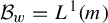 (see (A.2) for
$h=1$
 ). The same comment applies for other conditions in [Reference Dragičević and Hafouta19, Theorem 2].
Thus, it is necessary to combine the approach from [Reference Dragičević and Hafouta19] with the cone techniques used in the study of LSV maps initiated in [Reference Liverani, Saussol and Vaienti31].
We emphasize that the proof of Theorem 9 actually requires a certain improvement of the linear response result of [Reference Dragičević, Gonzalez-Tokman and Sedro17] (see Theorem 6 and Remark 7) and that contrary to [Reference Sélley35], it yields an explicit formula for the derivative of the variance (see Remark 10). However, Theorem 9 does require (in comparison with Theorems 3 and 5) an additional constraint for the range of parameter values of the LSV maps. Unfortunately, we currently do not see a possible way to eliminate this constraint. We refer the reader to Remark 10 for further discussion on this issue.
Convention
Throughout this work, C and D will denote positive constants whose precise values may change from one appearance to the next. Dependence on parameters such as
$\alpha $
 will be indicated with subscripts, e.g.
$C=C_\alpha $
 , as needed.
2 Quenched central limit theorem for random LSV maps
Throughout this paper,
$(\Omega , \mathcal F, \mathbb P)$
 is an arbitrary probability space equipped with an invertible
$\mathbb P$
 -preserving transformation
$\sigma \colon \Omega \to \Omega $
 . We assume that
$\mathbb P$
 is ergodic. Moreover, m will denote the Lebesgue measure on the unit interval
$[0, 1]$
 . We recall that for each
$\gamma \in (0, 1)$
 , the associated Liverani–Saussol–Vaienti (LSV) map (introduced in [Reference Liverani, Saussol and Vaienti31]) is given by

Moreover, for
$\gamma \in (0, 1)$
 and an observable
$\phi $
 , we set

where
$g_\gamma $
 denotes the inverse of the restriction of
$T_\gamma $
 to
$[0, \frac 1 2]$
 . Finally, we will also denote
$v_\gamma (x):=\partial _\gamma T_\gamma (x)=2^\gamma x^{1+\gamma }\log (2x)$
 and

For each
$\omega \in \Omega $
 , let
$T_\omega \colon [0, 1] \to [0, 1]$
 be an LSV map with the parameter
$\beta (\omega ) \in (0, 1)$
 . As usual, we set

In the same manner, denoting by
$\mathcal L_\omega \colon L^1(m)\to L^1(m)$
 the transfer operator associated to
$T_\omega $
 and m, we set

We also set
$\mathcal L_\omega ^0 :=\textrm {Id}$
 for
$\omega \in \Omega $
 . In the following, we will assume that
$\omega \mapsto \beta (\omega )$
 is measurable and that

It is proved in [Reference Dragičević, Gonzalez-Tokman and Sedro17, Proposition 9] that the cocycle of maps
$(T_\omega )_{\omega \in \Omega }$
 admits a unique random absolutely continuous invariant measure (a.c.i.m.)
$\mu $
 on
$\Omega \times [0, 1]$
 , which can be identified with a family of probability measures
$(\mu _\omega )_{\omega \in \Omega }$
 on
$[0, 1]$
 such that

Moreover,
$d\mu _\omega =h_\omega \, dm$
 with
$h_\omega \in \mathcal C_*\cap \mathcal C_2$
 for some
$a>1$
 , where
$\mathcal C_*=\mathcal C_*(a)$
 and
${\mathcal C_2=\mathcal C_2(b_1, b_2)}$
 are cones as in [Reference Dragičević, Gonzalez-Tokman and Sedro17, §2.2], that is,
$\mathcal C_*$
 consist of
$\phi \in C^0(0, 1]\cap L^1(m)$
 such that
$\phi \ge 0$
 ,
$\phi $
 decreasing,
$X^{\alpha +1}\phi $
 increasing (where X denotes the identity map), and

Moreover,
$\mathcal C_2$
 consists of all
$\phi \in C^2(0, 1]$
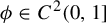 so that

We stress that the parameters a,
$b_1$
 , and
$b_2$
 depend only on
$\alpha $
 . Throughout the paper, we will often use the following simple result.
If
$h\in \mathcal C_*$
 and
$\varphi \in C^1[0, 1]$
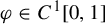 , then by [Reference Leppänen and Stenlund30, Lemma 3.3] (see also [Reference Nicol, Török and Vaienti33, Remark 2.5] and [Reference Nicol, Perez Pereira and Török32, Lemma 3.4]),

for
$g_1,g_2 \in {\mathcal {C}}_*$
 with
$\Vert g_i \Vert _{L^1(m)} \le C_\alpha \Vert \varphi \Vert _{C^1} \Vert h \Vert _{L^1(m)}$
 for
$i = 1,2$
 . Moreover, if
$h \in C(0,1]$
 , then
$g_i \in C^1(0,1]$
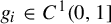 .
Proposition 1. There exists
$C_\alpha>0$
 such that

for
$\mathbb P$
 -a.e.
$\omega \in \Omega $
 ,
$n\in \mathbb N$
 , and
$\varphi \in C^1[0, 1]$
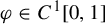 ,
$h\in \mathcal C_*$
 with
$\int _0^1 \varphi h\, dm=0$
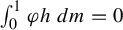 .
Proposition 2. Suppose that
$\psi \in C^1(0,1]$
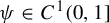 satisfies
$\int _0^1 \psi \, d m = 0$
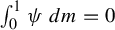 and, for
$x \in (0,1]$
 ,

where
$0 < \gamma \le \alpha $
 and
$C_0,C_1> 0$
 . Then, there exists
$C=C_{a, \alpha , \gamma }>0$
 such that, for
${\mathbb {P}}$
 -a.e.
$\omega \in \Omega $
 ,

holds for
$n \in \mathbb {N}$
 . In particular, if
$\varphi \in C^1[0, 1]$
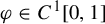 satisfies
$\int _0^1 \varphi h_\omega \, dm = 0$
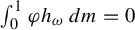 for
${\mathbb {P}}$
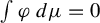
 -a.e.
$\omega \in \Omega $
 , and

where
$\gamma \ge 0$
 , then there exists a constant
$C=C_{a, \alpha , \gamma }> 0$
 such that, for
${\mathbb {P}}$
 -a.e.
$\omega \in \Omega $
 ,

holds for
$n \in \mathbb {N}$
 .
Proof. Denote by
${\mathcal {C}}_*(a; \gamma )$
 the cone obtained by replacing
$\alpha $
 with
$\gamma $
 in the definition of
$\mathcal C_*$
 . It follows from [Reference Dragičević, Gonzalez-Tokman and Sedro17, Lemma 3] or [Reference Leppänen29, Lemma 3.3] that (note that although
$F \in C^2(0,1]$
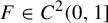 is assumed in [Reference Dragičević, Gonzalez-Tokman and Sedro17, Lemma 3], the proof only uses
$F \in C^1(0,1]$
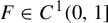 )

where
$\psi _{i} \in {\mathcal {C}}_*(a; \gamma )$
 , provided that

If
$\int _0^1 \psi _{ 1} \, dm = 0$
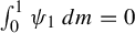 , then
$\psi _1(x) = 0$
 for m-a.e.
$x \in [0,1]$
 and (3) holds trivially. Otherwise, let
$\tilde {\nu }_{i}$
 denote the probability measure with density
$\tilde {\psi }_{ i} = \psi _{ i} / \int _0^1 \psi _{ i} \, dm \in {\mathcal {C}}_*(a; \gamma )$
 . Then,
$\tilde {\nu }_{i}$
 is regular in the sense of [Reference Korepanov and Leppänen26, Definition 3.5]; see [Reference Korepanov and Leppänen26, Proposition 3.14]. Moreover, the first entry time

satisfies

In the terminology of [Reference Korepanov and Leppänen26], this means that
$\tilde {\nu }_{i}$
 has tail bound
$C_{a,\gamma , \alpha } n^{- 1 / \alpha + \gamma / \alpha }$
 . Note that

Now, (3) follows from [Reference Korepanov and Leppänen26, Theorem 3.8], and (4) is a straightforward consequence of (3) using
$h_\omega \in {\mathcal {C}}_* \cap {\mathcal {C}}_2$
 .
We are now in a position to state and prove our quenched central limit theorem for random compositions of LSV maps.
Theorem 3. Let
$\Phi \colon \Omega \times [0, 1] \to \mathbb R$
 be a measurable map such that
$\varphi _\omega :=\Phi (\omega , \cdot )\in C^1[0, 1]$
 for
$\omega \in \Omega $
 and that

Moreover, assume that one of the following two conditions holds:
-
(i) $\alpha < 1/2$
 ;
-
(ii) $\alpha \ge 1/2$
and, for
$x \in [0,1]$
and
${\mathbb {P}}$
-a.e.
$\omega \in \Omega $
, (6) $$ \begin{align} |\varphi_\omega(x)| \le C_\omega x^{\gamma} \quad \text{and} \quad \int_0^1 \varphi_\omega h_\omega \, dm = 0 \end{align} $$hold with $\gamma> 2 \alpha - 1$
, where
$\omega \mapsto C_\omega \in L^2(\Omega , \mathcal {F}, {\mathbb {P}})$
.



Then, for
$\mathbb P$
 -a.e.
$\omega \in \Omega $
 ,

where

and
$\varphi _{\omega , 0}:=\varphi _\omega -\int _0^1 \varphi _\omega h_\omega \, dm$
 . Here,
$\mathcal N(0, \Sigma ^2)$
 denotes the normal distribution with mean
$0$
 and variance
$\Sigma ^2$
 provided that
$\Sigma ^2>0$
 , and the unit mass in
$0$
 in the case
$\Sigma ^2=0$
 .
Proof. First, we assume that condition (i) holds. We will verify the assumptions of [Reference Kifer25, Theorem 2.3.] with
$Q=\Omega $
 (that is, when there is no inducing involved) and with the fiberwise centered observable. Note that
$\varphi _{\omega , 0} \in C^1[0, 1]$
 for
$\omega \in \Omega $
 . Since

we have that
$\|\varphi _{\omega , 0}\|_{C^1}\le 2\|\varphi _\omega \|_{C^1}$
 , and thus from (5), we get that

Observing that
$(\mathbb E_{\mu _\omega }|\varphi _{\omega , 0}|^2)^{1/2}\le \|\varphi _{\omega , 0}\|_{C^1}$
 , we see that (7) implies [Reference Kifer25, (2.7)].
Next, we aim to verify that [Reference Kifer25, Theorem 2.3(i)] is true. Using (A.2), we have that

Consequently, using Hölder’s inequality and that
$\sigma $
 preserves
$\mathbb P$
 , we have that

which is finite due to (7) and
$\alpha <1/2$
 .
It remains to verify [Reference Kifer25, Theorem 2.3(ii’)]. More precisely, we need to show that

where

for
$\omega \in \Omega $
 and
$n\in \mathbb N$
 . In addition,
$L_\omega ^0:=\textrm {Id}$
 . Note that

for
$\omega \in \Omega $
 and
$n\in \mathbb N$
 . Then, by relying on (A.2) again, we see that

Therefore, using the fact that
$\sigma $
 preserves
$\mathbb P$
 , we have

which is finite due to (7) and
$\alpha <\frac 1 2$
 . The proof of condition (i) is complete.
The proof in the case of condition (ii) is similar to that of condition (i) and proceeds via an application of [Reference Kifer25, Theorem 2.3] relying on (4). To avoid repetition, we only give an outline of the proof. Note that
$\varphi _{\omega , 0}=\varphi _\omega $
 . Assuming condition (ii), we obtain [Reference Kifer25, (2.7)] using (5) since
$(\mathbb E_{\mu _\omega }|\varphi _{\omega }|^2)^{1/2}\le \|\varphi _\omega \|_{C^1}$
 . Arguing as in (8), using (4) and (6), we obtain

for
${\mathbb {P}}$
 -a.e.
$\omega \in \Omega $
 , where
$C> 0$
 depends only on
$a, \alpha , \gamma $
 . Consequently,

since
$\alpha < (1 + \gamma ) / 2$
 . Hence, [Reference Kifer25, Theorem 2.3(i)] holds. Finally, [Reference Kifer25, Theorem 2.3(ii’)] follows by a computation similar to (10), but using (4) instead of (A.2) to obtain

Remark 4.
-
(1) In the case where $(\Omega , \sigma )$
is a full shift,
$\mathbb P$
is an ergodic invariant measure for
$\sigma $
, and
$\varphi _\omega $
are Lipschitz continuous with Lipschitz constants uniformly bounded in
$\omega $
, Theorem 3(i) was established in [Reference Su36, Corollary 3.8] (extending the previous results [Reference Nicol, Perez Pereira and Török32, Reference Nicol, Török and Vaienti33]). -
(2) The proof of Theorem 3 yields a stronger conclusion, namely that the quenched law of iterated logarithm holds, provided that $\Sigma ^2>0$
(see the statement of [Reference Kifer25, Theorem 2.3]). -
(3) To the best of our knowledge, Theorem 3(ii) is new in the setting of random dynamics. For a single LSV map $T_\alpha $
with parameter
$1/2 < \alpha < 1$
and absolutely continuous invariant probability measure
$\mu $
, Gouëzel [Reference Gouëzel22] proved that
$n^{-1/2} \sum _{j=0}^{n-1} \varphi \circ T_\alpha ^n$
converges weakly to a normal distribution on
$([0,1], \mu )$
, provided that
$\varphi $
is Hölder continuous with
$\int \varphi \, d \mu = 0$
and
$|\varphi (x)| \le C x^\gamma $
holds for
$\gamma> \alpha - 1/2$
. A corresponding weak invariance principle was proved by Dedecker and Merlevède [Reference Dedecker and Merlevède13]. -
(4) We present a simple class of examples of observables $\Phi $
satisfying (6). To this end, take
$C^1$
functions
$u, g\colon [0, 1]\to \mathbb R$
such that $$ \begin{align*} 0\le u(x)\le Kx^\gamma, \quad x\in [0, 1], \end{align*} $$where $\gamma>2\alpha -1$
and u is not identically zero. Define now
$\Phi \colon \Omega \times [0, 1]\to \mathbb R$
by $$ \begin{align*} \varphi_\omega=\Phi(\omega, \cdot):=u (g-c_\omega), \quad \omega \in \Omega, \end{align*} $$where
$$ \begin{align*} c_\omega:=\frac{\int_0^1 gu\, d\mu_\omega}{\int_0^1u\, d\mu_\omega}, \quad \omega \in \Omega. \end{align*} $$We note that $c_\omega $
is well defined for
$\mathbb P$
-a.e.
$\omega \in \Omega $
. Indeed, we recall that it was established in the proof of [Reference Dragičević, Gonzalez-Tokman and Sedro17, Proposition 9] that there is
$\rho>0$
such that for
$\mathbb P$
-a.e.
$\omega \in \Omega $
,
$h_\omega \ge \rho \, m$
-almost everywhere. Hence, $$ \begin{align*} \int_0^1 u\, d\mu_\omega \ge \rho \int_0^1u\, dm>0 \quad \text{for } \mathbb P\text{-a.e. } \omega \in \Omega. \end{align*} $$In addition,
$$ \begin{align*} |c_\omega|\le \frac{|\int_0^1 gu\, d\mu_\omega|}{\int_0^1 u\, d\mu_\omega}\le \frac{\|g\|_\infty \int_0^1 u\, d\mu_\omega}{\int_0^1 u\, d\mu_\omega}=\|g\|_\infty \quad \text{for } \mathbb P\text{-a.e. } \omega \in \Omega. \end{align*} $$Therefore,
$$ \begin{align*} |\varphi_\omega(x)|=|u(x)| \cdot |g(x)-c_\omega|\le 2 Kx^\gamma \|g\|_\infty \quad \text{for } x\in [0, 1] \text{ and } \mathbb P\text{-a.e. } \omega \in \Omega. \end{align*} $$Thus, the first requirement in (6) holds with $C_\omega :=2K\|g\|_\infty $
for
$\mathbb P$
-a.e.
$\omega \in \Omega $
. Clearly, the second requirement in (6) is also fulfilled.




















3 Continuity of the variance
We are interested in studying the regularity of the variance
$\Sigma ^2$
 in Theorem 3 under suitable perturbations of random dynamics.
Let us start by introducing the appropriate setup. We take
$\varepsilon _0>0$
 , and measurable maps
$\beta \colon \Omega \to (0, 1)$
 and
$\delta \colon \Omega \to (0, 1)$
 such that

For
$\omega \in \Omega $
 and
$\varepsilon \in (-\varepsilon _0, \varepsilon _0)$
 , let
$T_{\omega , \varepsilon }$
 be an LSV map with parameter
$\beta (\omega )+\varepsilon \delta (\omega )$
 . We will write
$T_{\omega }$
 instead of
$T_{\omega , 0}$
 . By
$\mathcal L_{\omega , \varepsilon }$
 , we will denote the transfer operator associated with
$T_{\omega , \varepsilon }$
 , again writing
$\mathcal L_\omega $
 instead of
$\mathcal L_{\omega , 0}$
 . By
$(\mu _{\omega , \varepsilon })_{\omega \in \Omega }$
 , we will denote the random a.c.i.m. associated with the cocycle
$(T_{\omega , \varepsilon })_{\omega \in \Omega }$
 . We will write
$\mu _\omega $
 instead of
$\mu _{\omega , 0}$
 . By
$h_{\omega , \varepsilon }\in \mathcal C_*\cap \mathcal C_2$
 , we denote the density of
$\mu _{\omega , \varepsilon }$
 (again writing
$h_\omega $
 instead of
$h_{\omega , 0}$
 ).
Let
$F\colon \Omega \times [0, 1] \to \mathbb R$
 be a measurable map such that
$F(\omega , \cdot )\in C^1[0, 1]$
 for
$\omega \in \Omega $
 and

In the following, we will denote
$F_\omega :=F(\omega , \cdot )$
 . Set

Moreover, let

By Theorem 3,
$\Sigma _\varepsilon ^2$
 is finite for
$\varepsilon \in (-\varepsilon _0, \varepsilon _0)$
 . Then, we have the following theorem.
Theorem 5. The map
$\varepsilon \mapsto \Sigma _\varepsilon ^2$
 is continuous in
$0$
 .
Proof. We will first show that

To this end, observe that

Observe that for
$\mathbb P$
 -a.e.
$\omega \in \Omega $
 ,

and consequently,

where in the second inequality, we used Proposition A.3 and (11). However,

Consequently,

for
$\mathbb P$
 -a.e.
$\omega \in \Omega $
 . This implies that

yielding

Similarly,
$|f_{\omega , 0}^2|\le 4\|F_\omega \|_{C^0}^2$
 and thus, using Proposition A.3 and (11), we have

since

Therefore, we conclude that (13) holds.
Next, we observe that

where we used (A.2) and (11). Since the series
$\sum _{n=1}^\infty n^{-1/\alpha +1}$
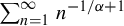 is summable, to prove our theorem, it remains to show that for each
$n\in \mathbb N$
 , the map

is continuous in
$0$
 . To this end, we first observe that

since
$f_{\sigma ^n \omega , \varepsilon }-f_{\sigma ^n \omega , 0}$
 depends only on
$\varepsilon $
 and
$\omega $
 (see (14)) and

Next,

Moreover,

where we used Proposition A.3. This together with (11) implies that

Finally, we have that

Therefore,

In addition, we have

since
$\partial _\gamma \mathcal L_\gamma (\phi )=-(X_\gamma N_\gamma (\phi ))'$
 (see [Reference Baladi and Todd9, p. 865]). It follows from
$h_\omega \in \mathcal C_*\cap \mathcal C_2$
 and (1) that, for
$\mathbb P$
 -a.e.
$\omega \in \Omega $
 , we have
$f_{\omega , 0}h_\omega =\psi _1-\psi _2$
 for some
$\psi _i=\psi _i(\omega )\in \mathcal C_*\cap C^1(0,1]$
 . Moreover,
$\|\psi _i\|_{L^1}\le K$
 for
$i=1, 2$
 , where K does not depend on
$\omega $
 . Hence,

Consequently,

where the last inequality is a consequence of bounds on
$X_\gamma $
 and
$X_\gamma '$
 in [Reference Baladi and Todd9, (2.3) and (2.4)], the invariance of
${\mathcal {C}}_* \cap C^1(0,1]$
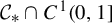 with respect to
$N_\gamma $
 and
${\mathcal {L}}_\gamma $
 (see [Reference Dragičević, Gonzalez-Tokman and Sedro17, Proposition 5]), and the observation (see [Reference Dragičević, Gonzalez-Tokman and Sedro17, Remark 1]) that

This gives that

for some
$C>0$
 independent on
$\varepsilon $
 . Thus,

This completes the proof of the theorem.
4 Differentiability of the variance
Take
$\beta \colon \Omega \to (0, 1)$
 ,
$\delta \colon \Omega \to [0, 1)$
 to be measurable maps and
$\underline {\alpha }>0$
 such that
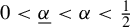
$0<\underline {\alpha }<\alpha <\frac 1 2$
 ,

Let
$T_{\omega , \varepsilon }$
 be the LSV map with parameter
$\beta (\omega )+\varepsilon \delta (\omega )$
 for every
$\omega \in \Omega $
 and
$\varepsilon \in (-\varepsilon _0, \varepsilon _0)$
 . By
$(\mu _{\omega , \varepsilon })_{\omega \in \Omega }$
 , we will denote the random a.c.i.m. that corresponds to the cocycle
$(T_{\omega , \varepsilon })_{\omega \in \Omega }$
 , where
$h_{\omega , \varepsilon }$
 is the density of
$\mu _{\omega , \varepsilon }$
 . As in the previous section, we will drop the subscript
$\varepsilon $
 when
$\varepsilon =0$
 .
We will use the following result, which is a sharper version of [Reference Dragičević, Gonzalez-Tokman and Sedro17, Theorem 14]. Its proof is given in Appendix C.
Theorem 6. There exists
$C=C_{\alpha , \underline {\alpha }}>0$
 such that for
$\varepsilon $
 sufficiently close to
$0$
 ,

for
$\mathbb P$
 -a.e.
$\omega \in \Omega $
 , where

Moreover,

Remark 7. In Theorem 6, we show for
$\mathbb P$
 -a.e.
$\omega \in \Omega $
 , the map
$ (-\varepsilon _0, \varepsilon _0)\ni \varepsilon \mapsto h_{\omega , \varepsilon }\in L^1(m)$
 is differentiable in
$\varepsilon =0$
 . However, in [Reference Dragičević, Gonzalez-Tokman and Sedro17, Theorem 14], a weaker statement is proved: for
$\mathbb P$
 -a.e.
$\omega \in \Omega $
 and
$\psi \in L^\infty (m)$
 , the map
$\varepsilon \mapsto \int _0^1\psi h_{\omega , \varepsilon }\, dm$
 is differentiable in
$\varepsilon =0$
 . For other quenched linear response results for different classes of random dynamics, we refer to [Reference Crimmins and Nakano12, Reference Dragičević, Giulietti and Sedro16, Reference Dragičević and Hafouta19, Reference Dragičević and Sedro20, Reference Sedro and Rugh34].
Remark 8. An anonymous referee raised a question about the possibility of obtaining higher order derivatives of the map
$\varepsilon \mapsto h_{\omega , \varepsilon }$
 in
$\varepsilon =0$
 . We emphasize that this problem has not been addressed in the case of autonomous dynamics yet. However, it is briefly mentioned in [Reference Baladi and Todd9, p. 859] that the cone approach developed in [Reference Baladi and Todd9] (used in [Reference Dragičević, Gonzalez-Tokman and Sedro17] and the present paper) is likely to yield such higher order regularity. However, it would require the construction of new families of invariant cones. In addition, we mention that if such a result holds, then it would have a somewhat different form than [Reference Crimmins and Nakano12, Theorem 3.6]. More precisely, unlike in [Reference Crimmins and Nakano12], where the quadratic response holds in the space weaker than that in which we have a linear response, in our setting, we should have both in
$L^1(m)$
 .
Let
$F\colon \Omega \times [0, 1] \to \mathbb R$
 be a measurable map such that
$F(\omega , \cdot )\in C^2[0, 1]$
 for
$\omega \in \Omega $
 and that

Let
$f_{\omega , \varepsilon }$
 and
$\Sigma _\varepsilon ^2$
 be as in the previous section. Then, we have the following theorem.
Theorem 9. Let
$\alpha <\frac 1 5$
 . Then, the map
$\varepsilon \mapsto \Sigma _\varepsilon ^2$
 is differentiable in
$0$
 .
Remark 10. We note that the proof of Theorem 9 yields

where
$L(\omega , F_\omega ):=\int _0^1 F_\omega \hat h_\omega \, dm$
 . The proof of Theorem 9 shows that this formula for the derivative of
$\Sigma _\varepsilon ^2$
 is well defined under the assumption
$\alpha < 1/5$
 . In particular, Lemma 18 ensures the summability

We do not know whether (20) remains valid beyond the range
$\alpha < 1/5$
 .
Remark 11. For a special class of observables as in Theorem 3(ii), we can weaken the constraint on
$\alpha $
 to
$\alpha < 1/4 + \delta $
 for suitable
$\delta> 0$
 . See Theorem 21 for a precise statement.
The proof of Theorem 9 will be established in a series of auxiliary results.
4.1 Differentiability of the first term in (12)
Lemma 12. The map

is differentiable in
$\varepsilon =0$
 .
Proof. Writing

it follows from (16) that

since

for
$\varepsilon $
 sufficiently close to
$0$
 . Next, we note that

as

for some
$C_{\alpha , F}>0$
 , where we used (14) and Proposition A.3. Finally,

since

for
$\varepsilon $
 sufficiently close to
$0$
 , where we used (14), Proposition A.3, and Theorem 6. Thus, the map in (21) is differentiable in
$\varepsilon =0$
 .
4.2 Differentiability of the second term in (12)
Next, we consider the second term in (12):

Let

and

Observe that

Consequently,

Let us now take
$\gamma \in (0, \frac 1 2)$
 such that

We note that this is possible since
$\alpha <\frac 1 4$
 . Then, we have

where
$C>0$
 is not dependent on
$\varepsilon $
 . Hence, due to (22), we have

Next, note that

since as in the proof of Theorem 5, we have

We first focus on
$D_n^2(\varepsilon )$
 . Taking into account (14) and

we have

Let

where
$L(\omega , F_\omega ):=\int _0^1 F_\omega \hat h_\omega \, dm$
 .
Lemma 13. We have

for
$\varepsilon $
 sufficiently close to
$0$
 .
Proof. Note that

Moreover,

for
$\mathbb P$
 -a.e.
$\omega \in \Omega $
 and
$\varepsilon $
 sufficiently close to
$0$
 , where we used Proposition A.3 and Theorem 6. Similarly,

for
$\mathbb P$
 -a.e.
$\omega \in \Omega $
 and
$\varepsilon $
 sufficiently close to
$0$
 . The conclusion of the lemma follows readily from the above estimates.
By Lemma 13, we have

Since
$ 1-2\alpha>\gamma $
 , we have

Taking into account (23), (24), and (25), to conclude the differentiability of
$\varepsilon \mapsto \Sigma ^2_\varepsilon $
 , it remains to establish the following.
-
• The limits $\lim _{\varepsilon \to 0} D_n^1(\varepsilon )$
and
$\lim _{\varepsilon \to 0}\bar D_n^2(\varepsilon )$
exist for each
$n \ge 1$
. -
• There exist $\bar {\varepsilon }_0> 0$
and
$u_n$
such that for all
$n < |\varepsilon |^{-\gamma }$
and all
$\varepsilon \in [-\bar {\varepsilon }_0, \bar {\varepsilon }_0]\setminus \{0\}$
, $$ \begin{align*} |D_n^1(\varepsilon)| \le u_n, \quad | \bar D_n^2(\varepsilon)|\le u_n \quad \text{and} \quad \sum_{n=1}^\infty u_n < \infty. \end{align*} $$
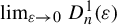




The first point above is established in Lemma 17 for
$\bar D_n^2$
 and in Lemma 19 for
$D_n^1$
 . The second point is proved in Lemma 16 for
$\bar D_n^2$
 and in Lemma 18 for
$D_n^1$
 .
4.3 A series of auxiliary lemmas
We write

Lemma 14. We have

Proof. Note that

Then, using that

we have

which yields the desired conclusion.
Lemma 15. We have

Proof. By using Theorem 6, we have

for
$r\in (0, 1)$
 that will be fixed later on. Next,

Since

we have using (A.2) that

In the same manner,

Moreover,

Observe that

In addition

By Theorem 6,

Furthermore,

and thus (taking into account (27)–(32)),

for r close to
$0$
 . In addition, since
$\int _0^1 f_{\omega , \varepsilon }h_{\omega , \varepsilon }\, dm=0$
 ,

which gives that

for
$n<|\varepsilon |^{-\gamma }$
 . By choosing
$r=n^{-({1-\alpha }/{\alpha (2-2\alpha )})}$
 (so that
$r^{1-2\alpha }=r^{-1}n^{-1/\alpha +1}$
 ), we obtain the desired conclusion.
As a direct consequence of the previous two lemmas and (26), we obtain the following lemmas.
Lemma 16. We have

Lemma 17. For each
$n\in \mathbb N$
 ,

Proof. We first show that

We start by decomposing

where
$k\in \mathbb N$
 . It follows from Theorem A.1 and Lemma A.2 that for
$\mathbb P$
 -a.e.
$\omega \in \Omega $
 ,

Thus, for
$k\in \mathbb N$
 ,

By
$h_\omega \in {\mathcal {C}}_* \cap {\mathcal {C}}_2$
 and Lemma A.2,

where
$\psi _1, \psi _2 \in {\mathcal {C}}_* \cap C^1(0,1]$
 . Hence, [Reference Leppänen and Stenlund30, Lemma 3.3] implies that

where
$\tilde {\psi }_{i,j} \in C^1(0,1] \cap {\mathcal {C}}_*$
 . Consequently,

Substituting (34) into the remaining expression and using
$\varphi (x + \varepsilon ) - \varphi (x) = \varepsilon \int _{0}^1 \varphi '( x + t \varepsilon ) \, dt$
 , we obtain

Moreover,

It follows from (15), bounds on
$X_\gamma $
 and
$X_\gamma '$
 in [Reference Baladi and Todd9, (2.3) and (2.4)], and invariance properties of the cones in (A.1) that

Consequently,

We choose
$k = \lfloor |\varepsilon |^{ - \alpha / ( 1 - \alpha ) } \rfloor $
 so that
$|\varepsilon | k$
 and
$k^{- 1 / \alpha + 2}$
 are approximately equal. Since
$\alpha < 1/2$
 ,

Hence, (33) holds.
We now claim that

Note that

By applying Lemma A.2, we conclude (using the convention
$0^{-1/\alpha +1}:=1$
 ) that

which easily implies (35). Finally, it remains to note that the conclusion of the lemma follows readily from (33) and (35).
We now consider
$D_n^1(\varepsilon )$
 and note that

Lemma 18. We have

Proof. Observe that

It follows from Lemmas B.2 and B.3 that

We now turn to
$D_{n,1}^1(\varepsilon )$
 . By definition,

where

For j such that
$n-j-1\ge \lfloor n/2\rfloor -1$
 , we have (using Lemma B.2 and Theorem A.1) that

We now consider j so that
$j\ge \lfloor n/2\rfloor $
 . For
$r>0$
 to be fixed later, we have by writing

and using Lemmas B.2 and B.3 that

Writing
$I_j$
 as

we have that

where we used that

Setting
$r=n^{-({1-\alpha })/{2\alpha }}$
 , it follows that

From (39) and (41), we conclude that

Observe that the upper bound in Lemma 16 is summable if
$\alpha < 1/4$
 , and the upper bound in Lemma 18 is summable if
$\alpha < 1/5$
 . To complete the proof of Theorem 9, it remains to prove the following lemma.
Lemma 19. We have

Proof. We decompose as in (37):

where
$\lim _{\varepsilon \to 0} D_{n, 2}^1(\varepsilon ) = 0$
 (see (38)). Next,

Furthermore,

Using Lemma A.2 together with Lemmas B.2 and B.4, we have

Hence,
$\lim _{\varepsilon \to 0} \mathcal D_{n, 2}^1(\varepsilon ) = 0$
 . This immediately implies the desired conclusion.
4.4 An improvement of Theorem 9 for a special class of observables
Here, we indicate how we can relax the assumption
$\alpha < 1/5$
 in the statement of Theorem 9 provided that we impose additional assumptions on F. We first note that the restriction
$\alpha < 1/5$
 is used only in Lemma 18; the rest of the proof remains valid under the weaker condition
$\alpha < 1/4$
 .
We continue to assume that
$F\colon \Omega \times [0, 1]\to \mathbb R$
 is measurable with
$F(\omega , \cdot )\in C^2[0, 1]$
 for
$\omega \in \Omega $
 and that (19) is valid. We need the following version of Lemma 18.
Lemma 20. Suppose that there exist
$0 \le \eta \le \alpha $
 and
$C>0$
 such that, for
${\mathbb {P}}$
 -a.e.
$\omega \in \Omega $
 and
$x \in [0,1]$
 ,

Then,

Proof. The proof proceeds as the proof of Lemma 18 up to (40). It follows from (4) that, for
${\mathbb {P}}$
 -a.e.
$\omega \in \Omega $
 ,

Thus, choosing
$r = n^{ \tfrac 12 ( 1 - ({1 + \eta })/{\alpha }) }$
 , we obtain

which yields (44).
Theorem 21. Suppose that (43) holds with
$0\le \eta \le \alpha $
 and
$C>0$
 . Provided that
${\alpha <({1+\eta })/{5}}$
 , we have that
$\varepsilon \mapsto \Sigma _\varepsilon ^2$
 is differentiable in
$\varepsilon =0$
 .
Acknowledgements
This paper has been funded by European Union – NextGenerationEU – Statistical properties of random dynamical systems and other contributions to mathematical analysis and probability theory (D.D). D.D is grateful to Yeor Hafouta for the ideas in [Reference Dragičević and Hafouta19] used in the present paper. J.L. is supported by JSPS under the project LEADER. He would like to thank the University of Rijeka for hospitality over the course of this work.
A Appendix
For the reader’s convenience, we gather in this section preliminary results from [Reference Dragičević, Gonzalez-Tokman and Sedro17] that are instrumental in the proofs of Theorems 5 and 9 concerning the regularity of the variance in the CLT.
Recall the definitions of the cones
${\mathcal {C}}_* = {\mathcal {C}}_*(a)$
 and
${\mathcal {C}}_2 = {\mathcal {C}}_2(b_1, b_2)$
 from §2. By [Reference Dragičević, Gonzalez-Tokman and Sedro17, Lemma 2 and Proposition 5], there exist
$a = a(\alpha )> 1$
 and
$b_1,b_2> 0$
 such that for
${0 < \beta \le \alpha }$
 , we have

The following theorem follows from [Reference Dragičević, Gonzalez-Tokman and Sedro17, Theorem 7].
Theorem A.1. There exists
$C_\alpha>0$
 with the property that for
$\mathbb P$
 -a.e.
$\omega \in \Omega $
 ,
$n\in \mathbb N$
 , and
$\phi , \psi \in \mathcal C_*$
 such that
$\int _0^1\phi \, dm=\int _0^1\psi \, dm$
 , we have

Furthermore, by [Reference Dragičević, Gonzalez-Tokman and Sedro17, Lemma 12], we have the following result.
Lemma A.2. For
$0<\gamma _0 \le \alpha <1$
 , there exist
$0<\delta \le \alpha $
 and
$C_1, C_2>0$
 such that

for
$x\in (0, 1]$
 ,
$\gamma \in [\gamma _0, \alpha ]$
 , and
$\phi \in \mathcal C_*(a)\cap \mathcal C_2(b_1, b_2)$
 with
$m(\phi )=1$
 . Moreover, there exist
$\psi _i \in \mathcal C_*(a)\cap C^1(0, 1]$
 ,
$i\in \{1, 2\}$
 such that

with
$\int _0^1 \psi _1 \, dm = \int _0^1 \psi _2\, dm$
 and
$\| \psi _i\|_{L^1(m)}\le D$
 ,
$i \in \{1, 2\}$
 for some
$D= D_{\gamma _0, \alpha }>0$
 .
The following result on statistical stability is a consequence of [Reference Dragičević, Gonzalez-Tokman and Sedro17, Theorem 13].
Proposition A.3. Let
$h_{\omega , \varepsilon }$
 be defined as in §3 with
$h_{\omega , 0} = h_\omega $
 . There exists
$C_\alpha>0$
 such that for
$\mathbb P$
 -a.e.
$\omega \in \Omega $
 ,

B Appendix
Lemma B.2. Let
$\varphi \in C^2$
 and
$h\in \mathcal C_*\cap \mathcal C_2$
 with
$\int _0^1 h\, dm=1$
 . Then, there exist
$\psi _i\in \mathcal C_*\cap \mathcal C_2$
 ,
$i=1, 2$
 such that

Moreover,
$\|\psi _i\|_{L^1(m)}\le D\|\varphi \|_{C^2}$
 for
$i=1, 2$
 , where D depends only on a,
$\alpha , b_1$
 , and
$b_2$
 (parameters of cones).
Proof. We recall the construction from [Reference Nicol, Perez Pereira and Török32]. Namely, take
$\psi _1=(\varphi +\unicode{x3bb} x+A)h+B$
 and
$\psi _2=(\unicode{x3bb} x+A)h+B$
 . Observe that (B.1) holds. Moreover, it is proved in [Reference Nicol, Perez Pereira and Török32] that
$\psi _1\in \mathcal C_*$
 provided that:
-
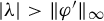
• $\unicode{x3bb} =-2\|\varphi \|_{C^1}$
(so that
$|\unicode{x3bb} |>\|\varphi '\|_{\infty }$
and
$\unicode{x3bb} <0$
); -
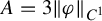
• $A=3\|\varphi \|_{C^1}$
so that
$\varphi +\unicode{x3bb} x+A\ge 0$
; -
• $B\ge ({a}/{(\alpha +1)})\|\varphi \|_{C^1}$
so that $$ \begin{align*} (\alpha+1)x^\alpha B\ge (\alpha+2)\unicode{x3bb} x^{\alpha+1}h(x)+x^{\alpha+1}h(x)\varphi'(x), \end{align*} $$where we also recall that $\unicode{x3bb} <0$
;
-
• $B\ge ({4a}/{(a-1)})\|\varphi \|_{C^1}$
, so that $$ \begin{align*} B\ge \frac{a}{a-1}[\sup(\varphi +\unicode{x3bb} x+A)]-\inf (\varphi+\unicode{x3bb} x+A)]. \end{align*} $$








Note that

Consequently,

provided that
$B\ge ({3a}/{b_1})\|\varphi \|_{C^1}$
 .
Next, note that

Thus,

provided that
$B\ge ({a}/{b_2})\|\varphi "\|_\infty +({6ab_1}/{b_2})\|\varphi \|_{C^1}$
 . Taking into account various conditions for B, we observe that we can choose B of the form
$B=d\|\varphi \|_{C^2}$
 , where constant
$d>0$
 depends only on
$\alpha , a, b_1$
 , and
$b_2$
 to fulfill these. With this choice, we have that
$\psi _1\in \mathcal C_2$
 . Finally, we observe that

which readily implies the desired conclusion.
Lemma B.3. Let
$0<\underline {\alpha }\le \alpha <1$
 . Then, there exist
$\delta =\delta (\underline {\alpha }, \alpha )\in (0, \alpha ]$
 such that

for any
$x\in (0, 1]$
 ,
$\gamma \in [\underline {\alpha }, \alpha ]$
 , and
$\phi \in \mathcal C_*\cap \mathcal C_2$
 . In particular,

Proof. The desired conclusion is obtained in the proof of [Reference Dragičević, Gonzalez-Tokman and Sedro17, Lemma 16], that is, in the arguments that yield the first estimate in [Reference Dragičević, Gonzalez-Tokman and Sedro17, (27)]. We note that these arguments do not use the assumption that
$\phi $
 belongs to the cone
$\mathcal C_3$
 made in the statement of [Reference Dragičević, Gonzalez-Tokman and Sedro17, Lemma 16].
Lemma B.4. Let
$0<\underline {\alpha }\le \alpha <1$
 . Then, there exist
$\delta =\delta (\underline {\alpha }, \alpha )\in (0, \alpha ]$
 such that

for
$x\in (0, 1]$
 ,
$\phi \in C^1(0, 1]\cap \mathcal C_*$
 , and
$\gamma \in [\underline {\alpha }, \alpha ]$
 . In particular,

Proof. The proof proceeds as the proof of [Reference Dragičević, Gonzalez-Tokman and Sedro17, Lemma 12] for verification of the first estimate in [Reference Dragičević, Gonzalez-Tokman and Sedro17, (15)]. The only difference concerns the term
$(N_\gamma (\phi ))'$
 , which in [Reference Dragičević, Gonzalez-Tokman and Sedro17] was handled by relying on the assumption that
$\phi \in \mathcal C_2$
 .
In the present context, assuming without loss of generality that
$\int _0^1\phi \, dm=1$
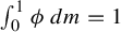 , we have
$N_\gamma (\phi )\in \mathcal C_*$
 (since
$\phi \in \mathcal C_*$
 ). Moreover,
$N_\gamma (\phi )\in C^1(0, 1]$
 as
$\phi \in C^1(0, 1]$
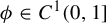 . Consequently, [Reference Dragičević, Gonzalez-Tokman and Sedro17, Remark 1] implies that

which is analogous to [Reference Dragičević, Gonzalez-Tokman and Sedro17, (18)].
C Appendix
Here, we provide the proof of Theorem 6. We stress that we closely follow the proof of [Reference Dragičević, Gonzalez-Tokman and Sedro17, Theorem 14].
Proof of Theorem 6
Using Theorem A.1 and Lemma A.2, it can easily be shown that the series in (17) converges in
$L^1(m)$
 for
$\mathbb P$
 -a.e.
$\omega \in \Omega $
 and that (18) holds.
For
$\mathbb P$
 -a.e.
$\omega \in \Omega $
 and each
$\varepsilon $
 , we have

for
$l\in \mathbb N$
 . Hence, Theorem A.1 implies that

Therefore, it follows that there exists
$l_0=l_0(\varepsilon )\in \mathbb N$
 such that for
$l\ge l_0$
 ,

However,

Writing

we see that

By Theorem A.1 and [Reference Dragičević, Gonzalez-Tokman and Sedro17, Lemma 16], we have that

However, similarly to [Reference Dragičević, Gonzalez-Tokman and Sedro17, Remark 21] for
$n=\lfloor |\varepsilon |^{-\alpha }\rfloor $
 and
$l>n$
 ,

Moreover,

where we used that in the proof of [Reference Dragičević, Gonzalez-Tokman and Sedro17, Theorem 14], it is showed that

for each
$1\le j\le n$
 . Next,

where we used (see [Reference Dragičević, Gonzalez-Tokman and Sedro17, Remark 21]) that (by making l sufficiently large)

for
$0\le j \le n$
 . The conclusion of the theorem follows by putting (C.1)–(C.5) together.


