2. Component importance for exchangeable lifetimes

Let $\varphi$ denote the structure function of a coherent system. Moreover, let $T_1, \dots, T_n$ denote the random variables which describe the component lifetimes in the considered system. In the following, we assume that the support of the distribution of each lifetime $T_i$ is given by the interval $[0, \infty)$ . The corresponding component states at time $t \geq 0$ are given by

\begin{equation*}X_{i}(t)={1}_{(t, \infty)}(T_i), \qquad i=1, \dots, n,\end{equation*}

with ${1}_{A}$ being the indicator function of the set A. This implies that the component state 1 indicates a working component (at time t) and 0 indicates a failed component (at time t). The vector of component states is denoted by $\textbf{\textit{X}}(t)=(X_{1}(t),\dots, X_{n}(t))$ .

Definition 1. cf. [Reference Birnbaum9] The time-dependent Birnbaum reliability importance of component i at a fixed time t is defined as

(1) \begin{align}I_\textrm{B}(i;\ t) &= \mathbb{P}(\varphi(\textbf{\textit{X}}(t))=1 \mid X_i(t)=1)-\mathbb{P}(\varphi(\textbf{\textit{X}}(t))=1 \mid X_i(t)=0).\end{align}

For arbitrary coherent systems, [Reference Eryilmaz24] obtained a representation of the preceding reliability importance for exchangeable lifetimes $T_1, \dots, T_n$ . Recall that the random vector $(T_1, T_2,\dots, T_n)$ is called exchangeable if its joint distribution coincides with that of any permutation of the random variables $T_1, T_2,\dots, T_n$ , i.e.

\begin{align*}\mathbb{P}(T_1 \leq t_1, T_2 \leq t_2, \dots, T_n \leq t_n)=\mathbb{P}(T_{\pi(1)} \leq t_1, T_{\pi(2)} \leq t_2, \dots, T_{\pi(n)} \leq t_n)\end{align*}

for every $t_1, \dots, t_n \in {\mathbb R}$ and any permutation $\pi$ of the numbers $1, \dots, n$ . Then, the reliability importance in (1) can be expressed as (see [Reference Eryilmaz24])

(2) \begin{align}I_\textrm{B}(i;\ t) &= \sum_{k=1}^n{\big[s_{k}^{+i}\mathbb{P}(T_{k\,{:}\,n}>t \mid T_i > t)- s_{k}^{-i}\mathbb{P}(T_{k\,{:}\,n}>t \mid T_i \le t)\big]},\end{align}

where $T_{1\,{:}\,n} \leq \dots \leq T_{n\,{:}\,n}$ are the order statistics of the random variables $T_1, \dots, T_n$ , and

(3) \begin{align} s_k^{+i} \coloneqq \frac{r_{n-k+1}^{+i}}{\binom{n-1}{n-k}} - \frac{r_{n-k}^{+i}}{\binom{n-1}{n-k-1}}, \quad k \in \{1,\dots, n-1\},\quad s_n^{+i} \coloneqq \frac{r_1^{+i}}{\binom{n-1}{0}}=r_1^{+i} ;\end{align}

(4) \hspace*{-78pt}\begin{align} s_k^{-i} \coloneqq \frac{r_{n-k+1}^{-i}}{\binom{n-1}{n-k+1}} - \frac{r_{n-k}^{-i}}{\binom{n-1}{n-k}}, \quad k \in \{2,\dots,n\},\quad s_1^{-i} \coloneqq 0 \hspace*{78pt}\end{align}

for $i=1, \dots, n$ . The parameters $r_k^{+i}$ and $r_k^{-i}$ can be defined as the sums

\begin{align*}r_k^{+i} \coloneqq \sum_{\vert A \vert = k, i \in A} \varphi({1}_A(1),\dots,{1}_A(n)), \qquad r_k^{-i}\coloneqq\sum_{\vert A \vert = k, i \not\in A} \varphi({1}_A(1),\dots,{1}_A(n)),\end{align*}

ranging over sets $A \subset \{1, \dots, n\}$ , i.e. they denote the number of path sets of size k of the considered system which contain and do not contain the component i, respectively. In particular, $r_n^{-i}=0$ , $r_n^{+i}=1$ , and $r_0^{-i}=r_0^{+i}=0$ . Observe that the representation in (2) involves conditional probabilities of the order statistics of the component lifetimes given the state of a component lifetime at time t. These conditional probabilities are in most cases not directly given and require further investigation.

In the next theorem we give another representation of the Birnbaum reliability importance. The joint distribution of the component lifetimes enters into this representation solely via the marginal distributions of the corresponding order statistics. The distribution (survival) function of an order statistic $T_{i\,{:}\,n}$ of the $T_1,\dots,T_n$ is denoted by $F_{i:n}$ ( $\overline{F}_{i\,{:}\,n}=1-F_{i\,{:}\,n}$ ). Note that $F_{i\,{:}\,n}$ (and $\overline{F}_{i\,{:}\,n}$ ) can usually be easily evaluated (cf. Remarks 1 and 2).

Theorem 1. Let $T_1,\dots,T_n$ be the component lifetimes of a coherent system of order n. If $T_1,\dots,T_n$ are exchangeable, then

(5) \begin{align}I_\textrm{B}(i;\ t)&= \left(\sum_{j=1}^n{\overline{F}_{j\,{:}\,n}(t)}\right)^{-1} \sum_{k=1}^n{s_{k}^{+i}\left(\,\sum_{\mathclap{m=1}}^{k-1}{\overline{F}_{m\,{:}\,n}(t)+(n-k+1)\overline{F}_{k\,{:}\,n}(t)}\right)}\nonumber\\&\quad - \left(\sum_{j=1}^n{F_{j\,{:}\,n}(t)}\right)^{-1} \sum_{k=2}^n{s_{k}^{-i}\left((k-1)\overline{F}_{k\,{:}\,n}(t) - \sum_{m=1}^{k-1}{\overline{F}_{m\,{:}\,n}(t)}\right)}\end{align}

for $i =1, \dots, n$ and $t >0$ .

Proof. Let $\phi_{k\,{:}\,n}$ denote the coherent life function (see, e.g., [Reference Esary and Marshall27] or [6, p. 12]) of a k-out-of-n:F system, i.e. a coherent system which fails if and only if k or more of its components fail. Then $\phi_{k\,{:}\,n}(x_1, \dots, x_n)$ is invariant with respect to permutations of its arguments $x_1,\dots, x_n$ . Furthermore, by definition $T_{k\,{:}\,n}=\phi_{k\,{:}\,n}(T_1, \dots, T_n)$ holds. Now, for $i,k \in \{1, \dots, n\}$ , consider

\begin{align*}\mathbb{P}(T_{k\,{:}\,n}>t, T_i > t) &= \mathbb{E}({1}_{(t, \infty)}(T_{k\,{:}\,n}) \cdot {1}_{(t, \infty)}(T_i))\nonumber\\ &= \mathbb{E}({1}_{(t, \infty)}(\phi_{k\,{:}\,n}(T_1, \dots, T_n)) \cdot {1}_{(t, \infty)}(T_i)).\end{align*}

Since $T_1, \dots, T_n$ are exchangeable, we get

\begin{align*}\mathbb{P}(T_{k\,{:}\,n}>t, T_i > t) = \frac{1}{n}\sum_{m=1}^n \mathbb{E}({1}_{(t, \infty)}(\phi_{k\,{:}\,n}(T_1, \dots, T_n)) \cdot {1}_{(t, \infty)}(T_m)).\end{align*}

Thus, because

\begin{equation*} \sum_{m=1}^n {1}_{(t, \infty)}(T_m)= \sum_{m=1}^n {1}_{(t, \infty)}(T_{m\,{:}\,n}), \end{equation*}

we can further conclude that

\begin{align*}\mathbb{P}(T_{k\,{:}\,n}>t, T_i > t) = \frac{1}{n} \sum_{m=1}^n \mathbb{E}({1}_{(t, \infty)}(\phi_{k\,{:}\,n}(T_1, \dots, T_n)) \cdot {1}_{(t, \infty)}(T_{m\,{:}\,n})).\end{align*}

Consequently, we obtain

\begin{align*}\mathbb{P}(T_{k\,{:}\,n}>t, T_i > t) = \frac{1}{n}\sum_{m=1}^n{\mathbb{P}(T_{k\,{:}\,n}>t, T_{m\,{:}\,n} > t)}\end{align*}

for $i,k \in \{1, \dots, n\}$ . Analogously, it can be shown that

\begin{align*}\mathbb{P}(T_{k\,{:}\,n}>t, T_i \leq t) = \frac{1}{n}\sum_{m=1}^n{\mathbb{P}(T_{k\,{:}\,n}>t, T_{m\,{:}\,n} \leq t)},\qquad\mathbb{P}(T_i > t) = \frac{1}{n}\sum_{m=1}^n{\overline{F}_{m\,{:}\,n}(t)}.\end{align*}

Moreover, we have in general

\begin{align*}&\mathbb{P}(T_{k\,{:}\,n}>t, T_{m\,{:}\,n} > t)=\begin{cases}\overline{F}_{m\,{:}\,n}(t), &\text{ if } 1 \le m < k,\\[4pt] \overline{F}_{k\,{:}\,n}(t), &\text{ if } k \le m \le n,\end{cases}\end{align*}

and

\begin{align*}\mathbb{P}(T_{k\,{:}\,n}>t, T_{m\,{:}\,n} \le t) &= \overline{F}_{k\,{:}\,n}(t) - \mathbb{P}(T_{k\,{:}\,n}>t, T_{m\,{:}\,n} > t)\nonumber\\[4pt] &= \begin{cases}\overline{F}_{k\,{:}\,n}(t) - \overline{F}_{m\,{:}\,n}(t), &\text{ if } 1 \le m < k,\\[4pt] \qquad 0, &\text{ if } k \le m \le n.\end{cases}\end{align*}

By plugging the obtained expressions into (2), we get the stated representation. □

Remark 1. Considering independent and identically distributed (i.i.d.) lifetimes $T_1, \dots, T_n$ with marginal distribution function F, the distribution of a single order statistic $T_{k\,{:}\,n}$ , $k \in \{1, \dots, n\}$ , is given by

\begin{align*}F_{k\,{:}\,n}(t) = \sum_{i=k}^n{\binom{n}{i}\big(F(t)\big)^i\big(1-F(t)\big)^{n-i}}\end{align*}

as developed, e.g., in [Reference David and Nagaraja18, p. 9]. In this case, the representation in (5) solely depends on the distribution function of a single component.

Remark 2. The representation in Theorem 1 is primarily useful in situations where the distributions of the order statistics of the lifetimes $T_1,\dots,T_n$ are given in an accessible form. However, for other joint distributions it might be easier to find the marginal distributions of random variables $T_{1\,{:}\,i}=\min(T_1, \dots, T_i)$ , or alternatively $T_{i\,{:}\,i}=\max(T_1, \dots, T_i)$ , $i=1, \dots, n$ . In that case, Theorem 1 can still be used by applying the following relations for distributions of exchangeable random variables:

\begin{align*}F_{r\,{:}\,n}(t) &= \sum_{j=n-r+1}^n (\!-1)^{j-n+r-1} \binom{j-1}{n-r} \binom{n}{j} \, F_{1\,{:}\,j}(t)= \sum_{j=r}^n (\!-1)^{j-r} \binom{j-1}{r-1} \binom{n}{j} \, F_{j\,{:}\,j}(t)\end{align*}

(see, e.g., [Reference David and Nagaraja18, p. 46], or [Reference Navarro, Ruiz and Sandoval46, Proposition 4.1]; see also [Reference Eryilmaz24, Lemma 1]).

Originally, [Reference Birnbaum9] applied the importance measure to systems with independent components. Reference [Reference Barlow and Proschan6] used another representation of Birnbaum’s measure to define an importance measure for the case of dependent components. Both measures coincide when the components in the system are independent. For fixed t, the time-dependent version of the reliability importance of component i considered in Barlow and Proschan [Reference Barlow and Proschan6, p. 26, Eq. (1.10c), and Remark (c) on p. 27] (see also [Reference Kuo and Zhu37, pp. 346–347]) is defined by

(6) \begin{align}I_\textrm{B,\,BP}(i;\ t) = \mathbb{E}\big(\varphi(1_i,\textbf{\textit{X}}(t)) - \varphi(0_i,\textbf{\textit{X}}(t))\big),\end{align}

where for an arbitrary vector $\textbf{\textit{x}}= (x_1, \dots, x_n) \in {\mathbb R}^n$ the usual notation 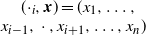$(\cdot_{i}, \textbf{\textit{x}})=(x_1,\dots,\break x_{i-1}, \, \cdot \, ,x_{i+1},\dots,x_n)$ is employed (cf. [6, p. 4]). In particular,

\begin{align*}(0_{i}, \textbf{\textit{x}})=(x_1,\dots,x_{i-1}, 0,x_{i+1},\dots,x_n),\qquad(1_{i}, \textbf{\textit{x}})=(x_1,\dots,x_{i-1}, 1 ,x_{i+1},\dots,x_n).\end{align*}

Clearly, if the component lifetimes or the component states are independent, then (1) and (6) are identical. Otherwise, both representations will usually lead to different values.

Remark 3. Note that the measure $I_\textrm{B,\,BP}(i;\ t)$ should not be confused with the Barlow-Proschan importance index

\begin{equation*} I_\textrm{BP}(i)=\mathbb{P}(T=T_i) \end{equation*}

from [Reference Barlow and Proschan5], where T denotes the system lifetime, which was also considered earlier as the Shapley–Shubik index in cooperative game theory (see, e.g., [Reference Marichal and Mathonet42] or [Reference Ramamurthy47, p. 75]). Moreover, if the component states are independent and, additionally,

\begin{equation*}\mathbb{P}(X_i(t)=1)=\frac{1}{2}, \qquad i=1, \dots, n,\end{equation*}

holds, then $I_\textrm{B}(i;\ t)=I_\textrm{B,\,BP}(i;\ t)$ and this value coincides with the structural importance of component i (see [Reference Barlow and Proschan6, p. 13, Eq. (3.10)]). In particular, the value has also been studied under the name absolute Banzhaf index in game theory (see, e.g., [Reference Ramamurthy47, p. 75]).

In the following theorem, we also give a representation of the importance measure (6) in terms of distribution functions of the ordered component lifetimes.

Theorem 2. Let $T_1,\dots,T_n$ be the component lifetimes of a coherent system of order n. If $T_1,\dots,T_n$ are exchangeable, then

(7) \begin{align}I_\textrm{B,\,BP}(i;\ t) = \frac{1}{n}\sum_{k=1}^n\big(s_{k}^{+i}-s_{k+1}^{-i}\big)\big((n-k)\overline{F}_{k\,{:}\,n}(t) + k \overline{F}_{k+1\,{:}\,n}(t)\big)\end{align}

for $i =1, \dots, n$ , $t >0$ with $s_{n+1}^{-i}\coloneqq 0$ , $\overline{F}_{n+1\,{:}\,n}\equiv 1$ .

Proof. For $i =1, \dots, n$ and $t >0$ , the considered importance measure can be expressed as

(8) \begin{align}I_\textrm{B,\,BP}(i;\ t) &= \mathbb{P}(\varphi(1_i,\textbf{\textit{X}}(t))=1) - \mathbb{P}(\varphi(0_i,\textbf{\textit{X}}(t))=1)\nonumber\\[4pt] &= [\mathbb{P}(T>t \mid T_i > t)- \mathbb{P}(\varphi(0_i,\textbf{\textit{X}}(t))=1 \mid X_i(t)=1)]\mathbb{P}(T_i > t)\nonumber\\[4pt] &\quad + [\mathbb{P}(\varphi(1_i,\textbf{\textit{X}}(t))=1 \mid X_i(t) = 0) - \mathbb{P}(T>t \mid T_i \le t)]\mathbb{P}(T_i \le t).\end{align}

In order to derive representations for the terms in (8), we will use arguments similar to those in [Reference Eryilmaz24]. According to equations (5) and (6) in that paper, we already know that

(9) \begin{align}\mathbb{P}(T>t \mid T_i > t) &= \sum_{k=1}^n s_k^{+i} \mathbb{P}(T_{k\,{:}\,n}>t \mid T_i > t), \end{align}

(10) \begin{align}\mathbb{P}(T>t \mid T_i \le t) &= \sum_{k=2}^n s_k^{-i} \mathbb{P}(T_{k\,{:}\,n}>t \mid T_i \leq t).\end{align}

To obtain the remaining terms in (8), consider at first

(11) \begin{align}\mathbb{P}(\varphi(0_i,\textbf{\textit{X}}(t))=1 \mid X_i(t)=1)=&\sum_{k=1}^n{\mathbb{P}(\varphi(0_i,\textbf{\textit{X}}(t))=1 \mid X_i(t)=1, S_n(t)=k)}\nonumber\\[3pt] & \times {\mathbb{P}(S_n(t)=k \mid T_i>t)},\end{align}

where $S_n(t)=\sum_{j=1}^n{X_j(t)}$ denotes the number of active components at time t. By introducing the set

\begin{align*}M_{\varphi}^{\mathcal{P},-i}& \coloneqq \big\{ \big({1}_{P'}(1),\dots,{1}_{P'}(n)\big) \in \{0,1\}^n \, \big \vert \nonumber\\&\qquad\qquad P' \subseteq \{1, \dots, n\}, P' \ni i, P'\setminus \{i\}\text{ is path set of } \varphi\big\},\end{align*}

we obtain

(12) \begin{align}\mathbb{P}(\varphi(0_i,\textbf{\textit{X}}(t))=1 \mid X_i(t)=1, S_n(t)=k) = \sum_{\mathclap{\substack{\textbf{\textit{x}} \in M_{\varphi}^{\mathcal{P},-i}\\\sum_{j=1}^n{x_j}=k}}}{\mathbb{P}( \textbf{\textit{X}}(t)=\textbf{\textit{x}} \, \big\vert \, X_i(t)=1,\,S_n(t)=k)}.\end{align}

Since exchangeability of the component lifetimes $T_1,\dots,T_n$ transfers to the states $X_1(t),\dots,X_n(t)$ , we get

\begin{align*}\mathbb{P}( \textbf{\textit{X}}(t)=\textbf{\textit{x}}_1 \, \vert \, X_i(t)=1,\,S_n(t)=k) = \mathbb{P}( \textbf{\textit{X}}(t)=\textbf{\textit{x}}_2 \, \vert \, X_i(t)=1,\,S_n(t)=k)\end{align*}

for all $\textbf{\textit{x}}_1,\textbf{\textit{x}}_2 \in B^{k,+i}_n \coloneqq \big\{ \textbf{\textit{x}}=(x_1, \dots,x_n) \in \{0,1\}^n \, \big\vert \, x_i = 1, \sum_{j=1}^n{x_j}=k\big\}$ , and hence

\begin{align*}\mathbb{P}\big( \textbf{\textit{X}}(t)=\textbf{\textit{x}} \, \big\vert \, X_i(t)=1,\,S_n(t)=k\big) = \frac{1}{\binom{n-1}{k-1}}\end{align*}

for every $\textbf{\textit{x}} \in B^{k,+i}_n$ , because the number of elements in this set is given by $|B^{k,+i}_n|=\binom{n-1}{k-1}$ . Therefore, it follows from (12) by using $\vert \{ \textbf{\textit{x}} \in M_{\varphi}^{\mathcal{P},-i}\mid x_i=1, \sum\nolimits_{j=1}^n{x_j}=k\}\vert = r_{k-1}^{-i}$ that

(13) \begin{align}\mathbb{P}(\varphi(0_i,\textbf{\textit{X}}(t))=1 \mid X_i(t)=1, S_n(t)=k)=\frac{r_{k-1}^{-i}}{\binom{n-1}{k-1}}.\end{align}

Furthermore, for $k\in \{1,\dots, n-1\}$ ,

\begin{align*}\mathbb{P}(S_n(t)=k\mid T_i >t) &= \mathbb{P}(T_{n-k+1\,{:}\,n} >t \mid T_i > t) - \mathbb{P}(T_{n-k\,{:}\,n} >t \mid T_i > t),\\[4pt] \mathbb{P}(S_n(t)=n \mid T_i >t) &= \mathbb{P}(T_{1\,{:}\,n} >t \mid T_i > t).\end{align*}

By plugging these expressions and (13) into (11), it can be shown after some calculations that

(14) \begin{align} \mathbb{P}\big(\varphi(0_i,\textbf{\textit{X}}(t))=1 \mid X_i(t)=1\big) = \sum_{k=1}^{n-1} s_{k+1}^{-i} \mathbb{P}(T_{k\,{:}\,n}>t \mid T_i > t).\end{align}

Applying a similar argument but now using the set

\begin{align*}M_{\varphi}^{\mathcal{P},+i}& \coloneqq \big\{ \big({1}_{P'}(1),\dots,{1}_{P'}(n)\big) \in \{0,1\}^n \, \big\vert \nonumber\\&\qquad\qquad P' \subseteq \{1, \dots, n\}\setminus \{i\},\, P'\cup \{i\} \text{ is path set of } \varphi\big\},\end{align*}

it can be proved that

(15) \begin{align}\mathbb{P}(\varphi(1_i,\textbf{\textit{X}}(t))=1 \mid X_i(t)=0, S_n(t)=k) = \frac{r^{+i}_{k+1}}{\binom{n-1}{k}}.\end{align}

Then, we obtain

(16) \begin{align}\mathbb{P}(\varphi(1_i,\textbf{\textit{X}}(t))=1 \mid X_i(t)=0) = \sum_{k=2}^{n+1}{s_{k-1}^{+i}\mathbb{P}(T_{k\,{:}\,n} >t \mid T_i \le t)},\end{align}

where $T_{n+1\,{:}\,n} \coloneqq \infty$ . Utilizing (9), (10), (14), and (16) in (8) (with $s_{n+1}^{-i} \coloneqq 0$ ) and arguing analogously to the proof of Theorem 1, we arrive at the representation in the theorem after some rearrangements. □

Remark 5. In a recent paper by Eryilmaz et al. [Reference Eryilmaz, Coolen and Coolen-Maturi26], a representation of the Birnbaum importance $I_\textrm{B}$ for systems with exchangeable components of $K\geq 2$ types is given. In the following, we add a corresponding representation for the measure $I_\textrm{B,\,BP}$ . Since no specific dependence between components of different types is assumed, the resulting expressions are clearly less tractable than in the case of only one type of exchangeable component. However, arguments similar to those used in [Reference Eryilmaz, Coolen and Coolen-Maturi26] and for showing Theorem 2 above can be applied. Consider a coherent system with n components of $K\geq 2$ types. The number of components of type v is denoted by $n_v$ , $1 \leq v \leq K$ , with $n=n_1+ \dots + n_K$ . Moreover, the lifetimes of the $n_v$ components of type v are denoted by random variables $T^{(v)}_1, \dots, T^{(v)}_{n_v}$ and the corresponding component states at time $t \geq 0$ by $X^{(v)}_1(t), \dots, X^{(v)}_{n_v}(t)$ . Assume that in the random vector of all component lifetimes the random lifetimes belonging to components of the same type are exchangeable dependent. Let $S^{(v)}_{n_v}(t)$ denote the number of active components of type v at time $t\geq 0$ . By arguing analogously to equations (9) and (10) of [Reference Eryilmaz, Coolen and Coolen-Maturi26], and deriving the coefficients similarly to equations (13) and (15) above, the following representation of the importance measure $I_\textrm{B,\,BP}(i;\ t)$ can be shown: If component i is of type a, then

\begin{equation*}I_\textrm{B,\,BP}(i;\ t)= \sum_{l_1=0}^{n_1} \dots \sum_{l_K=0}^{n_K} c_{n_1, \dots, n_K}(l_1, \dots, l_K) \mathbb{P}\big(S^{(1)}_{n_1}(t)=l_1, \dots, S^{(K)}_{n_K}(t)=l_K\big)\end{equation*}

with coefficients satisfying

\begin{multline*} c_{n_1, \dots, n_K}(l_1, \dots, l_K) \cdot \binom{n_1}{l_1} \cdots \binom{n_K}{l_K} \\[3pt] =\left[r^{+i}_{n_1, \dots, n_K}(l_1, \dots, l_K) + r^{+i}_{n_1, \dots, n_K}(l_1, \dots, l_a+1, \dots, l_K) \right. \\[3pt] \left. -r^{-i}_{n_1, \dots, n_K}(l_1, \dots, l_K) - r^{-i}_{n_1, \dots, n_K}(l_1, \dots, l_a-1, \dots, l_K)) \right],\end{multline*}

where we put

\begin{equation*}r^{+i}_{n_1, \dots, n_K}(l_1, \dots, l_{a-1}, 0, l_{a+1}, \dots, l_K)=r^{+i}_{n_1, \dots, n_K}(l_1, \dots, l_{a-1}, n_a+1, l_{a+1}, \dots, l_K)=0\end{equation*}

and $r^{-i}_{n_1, \dots, n_K}(l_1, \dots, l_{a-1}, -1, l_{a+1}, \dots, l_K)=0$ . Here, $r^{+i}_{n_1, \dots, n_K}(l_1, \dots, l_K)$ denotes the number of path sets of the system including component i of type a, $l_1$ components of type $1, \ldots ,l_a-1$ additional components of type ${a},\ldots,l_K$ components of type K, and $r^{-i}_{n_1, \dots, n_K}(l_1, \dots, l_K)$ denotes the number of path sets of the system that do not include component i of type a, and include $l_1$ components of type $1,\ldots,l_a$ components of type $a,\ldots,l_K$ components of type K (see [Reference Eryilmaz, Coolen and Coolen-Maturi26]). In particular,

\begin{equation*}r_{n_1, \dots, n_K}(l_1, \dots, l_K)=r^{+i}_{n_1, \dots, n_K}(l_1, \dots, l_K)+r^{-i}_{n_1, \dots, n_K}(l_1, \dots, l_K)\end{equation*}

holds, where $r_{n_1, \dots, n_K}(l_1, \dots, l_K)$ denotes the number of path sets of the system including exactly $l_1$ components of type $1,\ldots,$ exactly $l_K$ components of type K.

Moreover, the probabilities $\mathbb{P}(S^{(1)}_{n_1}(t)=l_1, \dots, S^{(K)}_{n_K}(t)=l_K)$ can be evaluated in terms of joint survival functions of the system lifetimes as follows (see [Reference Eryilmaz, Coolen and Coolen-Maturi26], Eq. (3)):

\begin{equation*}\mathbb{P}(S^{(1)}_{n_1}(t)=l_1, \dots, S^{(K)}_{n_K}(t)=l_K)= \binom{n_1}{l_1} \cdots \binom{n_K}{l_K} \cdot S_{n_1, \dots, n_K}(t;\ l_1, \dots, l_K) ,\end{equation*}

where

\begin{align*} & S_{n_1, \dots, n_K}(t;\ l_1, \dots, l_K) \\[4pt] & \quad =\sum_{i_1=0}^{n_1-l_1} \dots \sum_{i_K=0}^{n_K-l_K} (\!-1)^{i_1+\dots+i_K} \binom{n_1-l_1}{i_1} \cdots \binom{n_K-l_K}{i_K} \\[4pt] & \qquad\quad \times \mathbb{P}\Big(T^{(1)}_1>t, \dots, T^{(1)}_{l_1+i_1}>t, \dots, T^{(K)}_1>t, \dots, T^{(K)}_{l_K+i_K}>t\Big).\end{align*}

For the case of i.i.d. component lifetimes $T_1, \dots, T_n$ , [Reference Eryilmaz24] establishes a representation of the importance measure (1) based on survival functions of order statistics with sample size $n-1$ . The corollary below shows that this representation continues to hold for exchangeable lifetimes when definition (6) is applied.

Corollary 1. Let $T_1,\dots,T_n$ be the component lifetimes of a coherent system of order $n \geq 2$ . If $T_1,\dots,T_n$ are exchangeable, then

\begin{align*}I_\textrm{B,\,BP}(i;\ t)=&\sum_{k=1}^n \big(s_{k}^{+i} \overline{F}_{k\,{:}\,n-1}(t) -s_{k}^{-i} \overline{F}_{k-1\,{:}\,n-1}(t)\big)\end{align*}

for $i =1, \dots, n$ and $t >0$ , where $\overline{F}_{0\,{:}\,n-1}\equiv 0$ , $\overline{F}_{n:n-1}\equiv 1$ .

Proof. The result follows from Theorem 2 and the well-known triangle rule for distribution functions $F_{k\,{:}\,n-1} = \frac{n-k}{n} F_{k\,{:}\,n} + \frac{k}{n} F_{k+1\,{:}\,n}$ , $1 \leq k<n$ , of order statistics based on exchangeable random variables $T_1,\dots,T_n$ (cf., e.g., [Reference David and Joshi17]). □

The coefficients $s_{k}^{+i}$ and $s_{k}^{-i}$ have properties similar to the entries of the well-known signature vector (see, e.g., [Reference Samaniego48]) of a coherent system. For example, in [Reference Eryilmaz24] it is shown that

(17) \begin{align}\sum_{k=1}^n s_k^{+i}=1, \qquad \sum_{k=1}^n s_k^{-i}=\begin{cases}1, & \text{if there exists\,\, $k\ :\ s_k^{-i} \not=0$}, \\[4pt] 0, & \text{otherwise}.\end{cases}\end{align}

Moreover, the following lemma yields that the coefficients are also non-negative. Therefore, they can be interpreted as probability mass functions of a discrete distribution (at least if there is some positive coefficient).

Lemma 1. The coefficients $s_{k}^{+i}$ and $s_{k}^{-i}$ given in (3) and (4) satisfy

\begin{equation*} s_{k}^{+i} \geq 0, \quad s_{k}^{-i}\geq 0, \qquad k=1, \dots, n.\end{equation*}

Proof. We will show the claim for $s_k^{+i}$ at first. By definition, $r_k^{+i}\ge 0$ for all $i,k \in \{1, \dots, n\}$ . Hence, we get immediately $s_n^{+i}=r_1^{+i}\ge 0$ . Furthermore,

\begin{align*}&s_k^{+i} \;\ge\; 0 \quad \text{for all}\ k \in \{1, \dots, n-1\} \\\Leftrightarrow\quad &\frac{r_{k+1}^{+i}}{\binom{n-1}{k}} - \frac{r_{k}^{+i}}{\binom{n-1}{k-1}} \;\ge\; 0 \quad \text{for all}\ k \in \{1, \dots, n-1\} \\\Leftrightarrow\quad &k \cdot r_{k+1}^{+i} \;\ge\; (n-k)\cdot r_{k}^{+i} \quad \text{for all}\ k \in \{1, \dots, n-1\}.\end{align*}

In the following, we will show the latter inequality. As in [Reference Kuo and Zhu37], let $\mathcal{P}_i(d)$ denote the set of path sets of size d containing component i. Note that

\begin{equation*} |\{ P \in \mathcal{P}_i(k+1) \, | \, P' \subset P\}|=n-k \end{equation*}

for all $P' \in \mathcal{P}_i(k)$ , because every path set of size k which contains component i can be extended to a path set of size $k+1$ by adding one of the remaining $n-k$ components. Then, we obtain

\begin{align*}(n-k) \cdot r^{+i}_{k} &=\sum_{P' \in \mathcal{P}_i(k)} |\{ P \in \mathcal{P}_i(k+1) \, | \, P' \subset P\}| = \sum_{P \in \mathcal{P}_i(k+1)} |\{ P' \in \mathcal{P}_i(k) \, | \, P' \subset P\}|\\[4pt] &\le \sum_{P \in \mathcal{P}_i(k+1)} |\{ P' \subset \{1, \dots, n\} \, | \, i \in P', |P'|=k, P' \subset P \}|\nonumber\\[4pt] &= k \cdot r_{k+1}^{+i},\end{align*}

since the number of subsets of size k, which contain the element i, of a set with $k+1$ elements including i is given by $\binom{k}{k-1}=k$ . For proving the assertion for $s_k^{-i}$ , just note that

\begin{equation*} s^{-i}_n = \frac{r^{-i}_1}{\binom{n-1}{1}} \geq 0, \qquad s^{-i}_1=0,\end{equation*}

and, furthermore, for all $k \in \{1, \dots, n-2\}$ ,

\begin{align*}s_k^{-i} \;\ge\; 0 \quad \text{for all}\ k \in \{2, \dots, n-1\} \quad\Leftrightarrow\quad (k+1) \cdot r_{k+1}^{-i} \;\ge\; (n-k-1)\cdot r_{k}^{-i}.\end{align*}

Therefore, the result can be proved by arguing similarly to the first case. □

The above representations can be effectively employed due to the well-developed distribution theory of order statistics (see Remarks 1 and 2). Let us consider the following elementary example.

Example 1. Consider a classic bridge system of order 5 (cf., e.g., [Reference Samaniego48, p. 9]). Then, as developed in [Reference Eryilmaz24],

\begin{alignat*}{4}&\textbf{\textit{s}}^{+3} &{}={}& \big(0, \textstyle{\frac{1}{3}}, \textstyle{\frac{2}{3}}, 0, 0\big), &&\quad \textbf{\textit{s}}^{-3} &{}={}& \big(0, 0, \textstyle{\frac{2}{3}},\textstyle{\frac{1}{3}}, 0\big),\\[4pt] &\textbf{\textit{s}}^{+i} &{}={}& \big(0, \textstyle{\frac{1}{6}}, \textstyle{\frac{7}{12}}, \textstyle{\frac{1}{4}}, 0\big), &&\quad \textbf{\textit{s}}^{-i} &{}={}& \big(0, \textstyle{\frac{1}{4}}, \textstyle{\frac{7}{12}}, \textstyle{\frac{1}{6}}, 0\big),\end{alignat*}

for $i = 1, 2, 4, 5$ . (Note that $\textbf{\textit{s}}^{-3}$ is actually affected by an arithmetic error in [Reference Eryilmaz24]).

Let $T_1,\dots, T_5$ be the component lifetimes of the system, which we assume follow a particular Marshall–Olkin exponential distribution (cf. [6, 43]), i.e. the joint survival function of $(T_1,\dots, T_5)$ is given by

\begin{align*}\overline{F}(t_1,\dots,t_5) = \exp\left\{-\lambda_1\sum_{i=1}^5{t_i}- \lambda_{12345} \max\{t_1,\dots, t_5\}\right\},\end{align*}

where $\lambda_1,\lambda_{12345} >0$ and $t_i \geq 0 $ , $i=1,\dots,5$ . Note that then $T_1,\dots, T_5$ are not independent, but exchangeable. Moreover, they are known to be associated. Using the representations from Theorems 1 and 2 and Remark 2, and

\begin{align*}\overline{F}_{1\,{:}\,j}(t) &= \mathbb{P}(\min\{T_1,\dots, T_j\}>t) = \mathbb{P}(T_1 > t, \dots, T_j > t)\\&= \overline{F}(\underbrace{t,\dots,t}_{\mathclap{j \textrm{ times}}},\underbrace{0,\dots,0}_{\mathclap{5-j \textrm{ times}}}) = \exp\left\{-(j\lambda_1 + \lambda_{12345})t\right\}\end{align*}

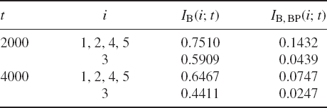
for $j=1, \dots 5$ , we are able to calculate $I_\textrm{B}(i;\ t)$ and $I_\textrm{B,\,BP}(i;\ t)$ for all components of the bridge system. Some exemplary values are given in Table 1.

Table 1:

Exemplary (rounded) values for the importance measures $I_\textrm{B}$ and $I_\textrm{B,\,BP}$ calculated in the setting of Example 1 with $\lambda_1 = 2\cdot 10^{-3}$ and $\lambda_{12345} = 4\cdot 10^{-3}$ .

3. Component importance for failure-dependent lifetimes

As an extended example, we will study so-called failure-dependent lifetimes based on the notion of the sequential order statistics defined in [Reference Kamps31]. In this model, after the failure of a component, the underlying lifetime distribution of the remaining components may change in order to take into account effects of previous failures. Failure-dependent component lifetimes are modeled with exchangeable random variables obtained via a random permutation of sequential order statistics. In this way, the model represents a framework for describing systems, where the performance of active components may be influenced by previous component failures (see [Reference Aki and Hirano1, Reference Burkschat10, Reference Navarro and Burkschat45]; see also [Reference Hollander29]). By construction, the order statistics of the failure-dependent component lifetimes coincide with sequential order statistics.

Note that the model of sequential order statistics can be applied to describe load-sharing scenarios in engineering applications, where the load of a failed component is distributed among the remaining active components. For modeling with sequential order statistics in this area, see, e.g, [4, 8, 15] and the references therein; see also [Reference Dewan and Naik-Nimbalkar21] and [Reference Kvam and Pena38] for general fields of applications.

In the following, let $T^*_{1\,{:}\,n},\ldots, T^*_{n\,{:}\,n}$ denote the sequential order statistics based on absolutely continuous distribution functions $F_1,F_2,\ldots,F_n$ with corresponding density functions $f_1,\ldots,f_n$ . Moreover, we denote the corresponding survival functions by $\overline{F}_i=1-F_i$ , $i=1, \dots, n$ .

Sequential order statistics can be introduced as follows (cf. [Reference Kamps31]; see also [Reference Burkschat and Navarro12]): Assume that the n components in a system start to work at time $t=0$ . The lifetimes of the components are described by independent random variables $T_1^{(1)}, T_2^{(1)}, \dots, T_n^{(1)}$ which are identically distributed according to the distribution function $F_1$ . The first failure time of a component is then given by

\begin{equation*}T_{1\,{:}\,n}^*=\min\big\{T_1^{(1)}, T_2^{(1)},\dots, T_n^{(1)}\big\}.\end{equation*}

Given that the first failure occurs at time $t_1=T_{1:n}^*$ , we assume that the residual lifetimes of the $n-1$ remaining components have the same distribution as the residual lifetimes of i.i.d. components with age $t_1$ and distribution function $F_2$ (instead of $F_1$ ). The distribution function $F_2$ is used to model the influence of the first component failure on the behavior of the other components. The lifetimes of these components will be represented by random variables $T_1^{(2)},T_2^{(2)}, \ldots, T_{n-1}^{(2)}$ . Given that $T_{1\,{:}\,n}^*=t_1$ , the random variables $T_1^{(2)},T_2^{(2)}, \ldots, T_{n-1}^{(2)}$ are i.i.d. according to the truncated distribution function $F_2(\cdot \mid t_1)$ with $\overline{F}_2(x \mid t_1)=\overline{F}_2(x)/\overline{F}_2(t_1)$ for $x\geq t_1$ . In particular, given that $T_{1\,{:}\,n}^*=t_1$ , these random variables satisfy $T_i^{(2)}\geq t_1$ for $i=1,2,\ldots,n-1$ . Then, the second failure time in the system is given by

\begin{equation*}T_{2\,{:}\,n}^*=\min\big\{T_1^{(2)}, T_2^{(2)},\dots, T_{n-1}^{(2)}\big\}.\end{equation*}

Proceeding in this way, we assume that the ith component failure occurs at time $t_i=T_{i\,{:}\,n}^*$ . Then we assume that the residual lifetimes of the $n-i$ remaining components have the same distribution as the residual lifetimes of i.i.d. components with age $t_i$ and distribution function $F_{i+1}$ . The distribution function $F_{i+1}$ describes the behavior of the remaining components after the occurrence of the ith failure. The lifetimes of the components will be represented by $T_1^{(i+1)}, T_2^{(i+1)}, \dots,T_{n-i}^{(i+1)}$ . Given that $T_{i\,{:}\,n}^*=t_i$ , the random variables $T_1^{(i+1)}, T_2^{(i+1)}, \dots,T_{n-i}^{(i+1)}$ are i.i.d. according to the truncated distribution function $F_{i+1}(\cdot \mid t_i)$ with $\overline{F}_{i+1}(x \mid t_i)=\overline{F}_{i+1}(x)/\overline{F}_{i+1}(t_i)$ for $x\geq t_i$ . Then, the $(i+1)$ th component failure time is

\begin{equation*}T_{i+1\,{:}\,n}^*=\min\Big(T_1^{(i+1)},T_2^{(i+1)},\ldots,T_{n-i}^{(i+1)}\Big).\end{equation*}

Finally, if the $(n-1)$ th component failure occurs at time $t_{n-1}=T_{n-1\,{:}\,n}^*$ , then the last failure time is given by $T_{n\,{:}\,n}^*$ with the reliability function $\overline{F}_{n}(x \mid t_{n-1})=\overline{F}_{n}(x)/\overline{F}_{n}(t_{n-1})$ for $x\geq t_{n-1}$ .

The formal definition of sequential order statistics can be found in [Reference Kamps31] (see also [Reference Cramer14, Reference Cramer and Kamps16]). In particular, the resulting joint density of the sequential order statistics $T^*_{1\,{:}\,n},\ldots, T^*_{n\,{:}\,n}$ is given by

\begin{align*}&f^{T^*_{1\,{:}\,n},\ldots, T^*_{n\,{:}\,n}}(t_1, \dots, t_n) = n! \left( \prod_{i=1}^{n-1} \left(\frac{1-F_i(t_i)}{1-F_{i+1}(t_i)}\right)^{n-i} f_i(t_i)\right) f_n(t_n) \end{align*}

for $t_1 \leq \dots \leq t_n$ , and is zero elsewhere. We will assume that the distribution functions satisfy

(18) \begin{align}F_i=1-(1-F)^{\alpha_i},\qquad i=1, \dots, n,\end{align}

based on an absolutely continuous distribution function F with density function f and parameters $\alpha_1,\dots,\alpha_n >0$ . This relation of the distribution functions often considered in the model of sequential order statistics is known as the proportional hazard rates (PHR) assumption, because then the corresponding hazard rates are given by

\begin{align*}\frac{f_i}{1-F_i}= \alpha_i\frac{f}{1-F}, \qquad i=1, \dots, n.\end{align*}

Under this assumption, increasingly ordered $\alpha_1 \leq \dots \leq \alpha_n$ correspond to a growing load on each individual component after every failure. In particular, the case of no additional stress on the components, i.e. $\alpha_1 = \dots = \alpha_n$ , leads to usual order statistics from an i.i.d. sample based on the distribution function $F_1$ . For convenience, in the remainder we will assume again that the support of the underlying F is given by $[0, \infty)$ .

Under the PHR assumption (18), well-known results on the marginal distributions (see [Reference Cramer and Kamps16, Reference Kamps and Cramer33]; see also [Reference Burkschat and Lenz11]) of generalized order statistics can be utilized in order to evaluate the importance measures of systems with failure-dependent components. For example, if the parameters $\gamma_i=\alpha_i(n-i+1)$ , $i=1, \dots, n$ , are pairwise different, i.e. $\gamma_k \not= \gamma_l$ for $k\not=l$ , then the distribution function of the rth sequential order statistic is given by

(19) \begin{align}F^{T^{*}_{r\,{:}\,n}}(t) &= 1- \left(\prod_{j=1}^r \gamma_j \right) \sum_{i=1}^r \frac{a_{i,r}}{\gamma_i}\left( 1-F(t)\right)^{\gamma_i},\end{align}

$t \geq 0,$ where

\begin{align*}\quad a_{i,r} \coloneqq \prod^r_{\substack{j=1\\j\not=i}} \frac{1}{\gamma_j-\gamma_i}, \qquad 1\leq i \leq r\leq n,\end{align*}

with $a_{1,1}=1$ . Moreover, for $\gamma_1 = \dots = \gamma_n$ , the corresponding distribution function is given by

(20) \begin{align} F^{T^{*}_{r\,{:}\,n}}(t) = 1- (1-F(t))^{\gamma_1} \sum_{j=0}^{r-1} \frac{1}{j!} (\!-\gamma_1 \ln(1-F(t)))^j,\end{align}

for $t \geq 0$ .

In case (a) the individual load on each component does not change with the number of failed units in the system. This case corresponds to the usual situation of i.i.d. component lifetimes. In case (b) the complete load of failed components is distributed evenly among the surviving ones. In this scenario, the total load on the system itself remains unchanged and the entirety of intact components is always stressed according to this initial load (cf., e.g., [Reference Balakrishnan, Beutner and Kamps4], Example 1). In particular, the first two cases can be considered as the possible extremal situations (cf., e.g., [Reference Burkschat and Navarro13], Remark 2.3). Consequently, the third case (c) can then be interpreted as an intermediate scenario between the previous two.

By applying representations (19) and (20) and exploiting that for this system the vectors of coefficients (3) and (4) belonging to components 1 and 2 are given by

\begin{align*}\textbf{\textit{s}}^{+1} &= (0,0,1,0), \quad \textbf{\textit{s}}^{-1} = (0,0,0,0), \quad \textbf{\textit{s}}^{+2}= \big(\textstyle{\frac{1}{3}},\textstyle{\frac{1}{3}},\textstyle{\frac{1}{3}},0\big), \quad \textbf{\textit{s}}^{-2} = \big(0, \textstyle{\frac{1}{3}},\textstyle{\frac{2}{3}}, 0\big),\end{align*}

we can evaluate the expressions for the importance measures given in this section. Note that, due to the structure of the system, the importance measures of components 3 and 4 coincide with those of component 2.

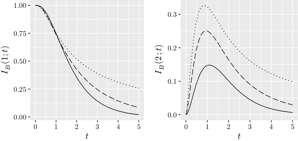
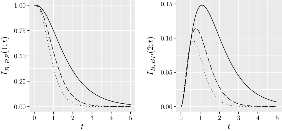
In Fig. 1 the importance measure $I_\textrm{B}$ given in (5) is displayed for components 1 and 2 in all three cases. Figure 2 shows the respective graphs for $I_\textrm{B,\,BP}$ given in (7).

Figure 1:

Plots of the importance measure $I_\textrm{B}$ given in (5) for the components with failure-dependent lifetimes based on the standard exponential distribution from Example 2 (component 1 is displayed on the left and component 2 on the right). The cases (a), (b), and (c) are depicted with solid, dotted, and dashed lines, respectively.

Figure 2:

Plots of the importance measure $I_\textrm{B,\,BP}$ given in (7) for the components with failure-dependent lifetimes based on the standard exponential distribution from Example 2 (component 1 is displayed on the left and component 2 on the right). The cases (a), (b), and (c) are depicted with solid, dotted, and dashed lines, respectively.

We point out that in case (a) both importance measures, $I_\textrm{B}$ and $I_\textrm{B,\,BP}$ , are identical (see Remark 4). It can be seen from the figures that the general shapes of the curves are also similar for both importance measures in the other considered situations. Moreover, the curves of $I_\textrm{B}$ always lie above the corresponding curves of $I_\textrm{B,\,BP}$ . This behavior will be explained in the next section (see Corollary 2). Furthermore, by studying the left graph in Fig. 1 in the interval $(0,1.5)$ and the right graph in Fig. 2 in the interval (0,1), it turns out that the curves cross each other in these areas. Therefore, although the parameter vectors $(\alpha_1, \dots, \alpha_4)$ are componentwise ordered in the three cases, these orderings are not transferred to the importance measures. As one may expect, it can be observed for larger t that the values of the importance measure in case (c) lie between the values of cases (a) and (b). It is also seen for such t that the importance measure $I_\textrm{B}$ assigns larger (smaller) values to the components in case (b) (case (a)), whereas the measure $I_\textrm{B,\,BP}$ shows the opposite behavior with smaller (larger) values in the respective cases.

4. Comparison of component importance

In this section we will show that the importance measures $I_\textrm{B}$ and $I_\textrm{B,\,BP}$ from the preceding section are ordered when the component lifetimes satisfy a suitable notion of dependence. For this reason, let us recall the following concepts of positive and negative dependence (see [Reference Barlow and Proschan6, Reference Esary, Proschan and Walkup28, Reference Joag-Dev and Proschan30]). Random variables $X_1, \dots, X_n$ are called associated if

\begin{equation*}\textrm{Cov}(g(X_1, \dots, X_n), h(X_1, \dots, X_n)) \geq 0\end{equation*}

for all increasing functions $g,h\colon{\mathbb R}^n \to {\mathbb R}$ for which the covariance exists; $X_1, \dots, X_n$ are called negatively associated if for all pairs of disjoint subsets $A_1,A_2 \subset \{1, \dots, n\}$ ,

\begin{equation*}\textrm{Cov}(g(X_i, i \in A_1), h(X_j, j \in A_2)) \leq 0\end{equation*}

for all increasing functions $g\colon{\mathbb R}^{|A_1|} \to {\mathbb R}$ , $h\colon{\mathbb R}^{|A_2|} \to {\mathbb R}$ for which the covariance exists. By applying these dependence concepts, we can establish the following ordering of the importance measures.

Theorem 3. Let $T_1, \dots, T_n$ be associated (negatively associated) component lifetimes. Then the importance measures $I_\textrm{B}$ and $I_{\textrm{B},BP}$ satisfy

\begin{equation*} I_\textrm{B}(i;\ t) \geq (\leq ) \, I_\textrm{B,\,BP}(i;\ t)\end{equation*}

for $i=1, \dots, n$ and every $t>0$ . In particular, $I_\textrm{B}(i;\ t)\geq 0$ holds for associated $T_1, \dots, T_n$ .

Proof. If the component lifetimes $T_1, \dots, T_n$ are associated (negatively associated), then the component states $X_{i}(t)={1}_{(t, \infty)}(T_i)$ are associated (negatively associated), too, as increasing functions of the component lifetimes. Thus, the representation

\begin{align*}I_\textrm{B}(i;\ t)-I_\textrm{B,\,BP}(i;\ t)=\frac{\textrm{Cov}(\varphi(1_i,\textbf{\textit{X}}(t)), X_{i}(t))}{\mathbb{E}(X_{i}(t))} -\frac{\textrm{Cov}(\varphi(0_i,\textbf{\textit{X}}(t)), 1-X_{i}(t))}{\mathbb{E}(1-X_{i}(t))}\end{align*}

yields the assertion, since the two included covariances $\textrm{Cov}(\varphi(1_i,\textbf{\textit{X}}(t)), X_{i}(t))$ and $\textrm{Cov}(\varphi(0_i,\textbf{\textit{X}}(t)), X_{i}(t))$ are non-negative (non-positive) due to the associated (negatively associated) component states. □

From the definitions (1) and (6), it follows immediately that $I_\textrm{B}(i;\ t) \leq 1$ and $0\leq I_\textrm{B,\,BP}(i;\ t)\break \leq 1$ . The preceding theorem provides a sufficient condition, namely association of the component lifetimes, which guarantees that $I_\textrm{B}$ is non-negative. The following example illustrates that $I_\textrm{B}$ can attain negative values in other situations.

Example 3. We examine the three-component system with structure function

\begin{equation*}\varphi(x_1, x_2 ,x_3) = \max(x_1, \min(x_2,x_3)), \end{equation*}

where $x_1,x_2,x_3 \in \{0,1\}$ . The coefficients (3) and (4) for this system are given by (cf. [Reference Eryilmaz24])

\begin{align*}\textbf{\textit{s}}^{+1}& = (0,0,1), \quad \textbf{\textit{s}}^{-1}= (0,1,0), \quad \textbf{\textit{s}}^{+2}= (0,1,0), \quad \textbf{\textit{s}}^{-2}=\big(0,\textstyle{\frac{1}{2}},\frac{1}{2}\big). \end{align*}

The components are assumed to be failure dependent based on distribution functions from the PHR model (18) with underlying standard exponential distribution. The occurring parameters are chosen as

\begin{equation*} \alpha_1=1,\ \alpha_2=\frac{2}{3},\ \alpha_3=\frac{1}{3}, \quad \text{i.e.} \ \gamma_1=3,\ \gamma_2=\frac{4}{3},\ \gamma_3=\frac{1}{3}. \end{equation*}

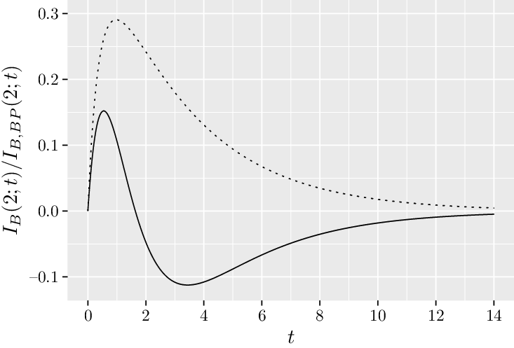
Therefore, in this scenario the individual load on each active unit is decreasing with the number of failed components. In Fig. 3 the resulting importance measures $I_\textrm{B}$ and $I_\textrm{B,\,BP}$ of component 2 are displayed. Clearly, the graphs for component 3 are the same.

It is apparent from Fig. 3 that $I_\textrm{B}(2;\ t)$ attains negative values for larger t. Since the lifetimes are negatively correlated in the situation considered (see [Reference Bezgina and Burkschat8]), it is possible that the failure of component 2 has a beneficial effect on the survival probability of the system. If the failure of component 2 occurs earlier (later) than t, then the lifetimes of the remaining components may tend to be larger (smaller) than t. In this way, conditioning with the event of a component failure before time t may lead to an increase of the probability that the remaining components, and consequently also the system, survive time t. While this phenomenon can become visible from $I_\textrm{B}$ (cf. definition (1)), it cannot be captured by $I_\textrm{B,\,BP}$ , which measures the gain in probability by switching from a defective component 2 to a flawless one, but does not take into account the influence of component 2 on the other components (cf. definition (6)). However, as a consequence, the usual interpretation of the Birnbaum importance as (positive) reliability growth does not necessarily hold anymore for the measure $I_\textrm{B}$ when facing dependence between the component lifetimes, whereas the measure $I_\textrm{B,\,BP}$ is not affected by that due to its construction.

In [Reference Bezgina and Burkschat8], dependence properties of failure-dependent lifetimes are examined. For example, from results on association of failure-dependent lifetimes, we can draw a conclusion for the important situation of an increasing load on surviving components (see also [Reference Shaked and Shanthikumar49], Section 6.1).

Figure 3:

Plots of importance measures $I_\textrm{B}(2;\ t)$ (solid) and $I_\textrm{B,\,BP}(2;\ t)$ (dotted) of component 2 for the system with failure-dependent lifetimes based on the standard exponential distribution from Example 3.

Corollary 2. Let $T^*_1, \dots, T^*_n$ be failure-dependent lifetimes and let the underlying distribution functions $F_1, \dots, F_n$ satisfy the PHR model (18) with an absolutely continuous F with continuous positive density f on $(0,\infty)$ . If $\alpha_1 \leq \dots \leq \alpha_n$ , then

\begin{equation*} 0 \leq I_\textrm{B,\,BP}(i;\ t) \leq I_\textrm{B}(i;\ t) \leq 1, \qquad i=1, \dots, n, \, t>0,\end{equation*}

holds for every coherent system of order n with component lifetimes $T^*_1, \dots, T^*_n$ .

Finally, we will compare the asymptotic behavior of both importance measures. The limiting behavior of $I_\textrm{B,\,BP}$ is directly seen as follows: As long as the lifetimes $T_1, \dots, T_n$ satisfy $T_i>0$ almost surely for $i=1, \dots, n$ , we obtain for the component states

\begin{equation*} \lim_{t \to 0+} X_i(t)=1, \quad \lim_{t \to \infty} X_i(t)=0, \qquad i=1, \dots, n,\end{equation*}

almost surely. Hence, since the structure function $\varphi$ can be chosen as a continuous function on $[0,1]^n$ , we conclude from (6) by using dominated convergence that

\begin{align*}\lim_{t \to 0+} I_\textrm{B,\,BP}(i;\ t) = 1-\varphi(0_i,\boldsymbol{1}),\qquad\lim_{t \to \infty} I_\textrm{B,\,BP}(i;\ t) = \varphi(1_i,\boldsymbol{0}),\end{align*}

where $\boldsymbol{0}= (0,\dots,0)$ and $\boldsymbol{1}= (1,\dots,1)$ . In particular, both limits are either equal to zero or one. More precisely,

\begin{align*}\lim_{t \to 0+} I_\textrm{B,\,BP}(i;\ t)=1 \, \, &\Leftrightarrow \, \, \text{$\{i\}$ is a (minimal) cut set,} \\\lim_{t \to \infty} I_{B,\,BP}(i;\ t)=1 \, \, &\Leftrightarrow \, \, \text{$\{i\}$ is a (minimal) path set.}\end{align*}

In order to study the limiting behavior of the measure $I_\textrm{B}$ , it will be helpful to state the connection between the above limits given in terms of the structure function $\varphi$ and the coefficients $s_k^{+i}$ and $s_k^{-i}$ from (3) and (4).

Proof. The second equality in (i) is given in (17). In order to obtain the first equality, note that it can be shown with (4) that

\begin{equation*}s_k^{-i}=0 \ \text{for all}\ k \in \{1, \dots, n\} \;\Leftrightarrow\; r_k^{-i}=0 \ \text{for all}\ k \in \{1, \dots, n\}, \end{equation*}

and with Lemma 1 it follows that

\begin{equation*}s_k^{-i}=0 \ \text{for all}\ k \in \{1, \dots, n\} \;\Leftrightarrow\; \sum_{k=1}^n{s_k^{-i}}=0.\end{equation*}

Consequently, the claimed equality follows by observing that

\begin{equation*} \varphi(0_i,\boldsymbol{1})= 0 \;\Leftrightarrow\; r_k^{-i}=0 \ \text{for all}\ k \in \{1, \dots, n\}. \end{equation*}

(ii) is obvious, because $\varphi(1_i,\boldsymbol{0})=1$ if and only if $r_1^{+i}=1$ . □

The limits of the importance measure $I_\textrm{B}$ depend on the tail behavior of the ordered component lifetimes. Here, we give explicit results for the failure-dependent lifetimes considered in Section 3.

Theorem 4. Let $T^*_1, \dots, T^*_n$ be failure-dependent lifetimes and let the underlying distribution functions $F_1, \dots, F_n$ satisfy the PHR model (18). The importance measure $I_\textrm{B}$ in (5) satisfies

\begin{align*} \lim_{t \to 0+} I_\textrm{B}(i;\ t)&=1-\varphi(0_i,\boldsymbol{1}) =\begin{cases}0, & if\ there\ exists\ k\,{:}\,s_k^{-i} \neq 0, \\[3pt] 1, & otherwise ; \end{cases}\\[3pt] \lim_{t \to \infty} I_\textrm{B}(i;\ t) & = \varphi(1_i,\boldsymbol{0})+ \Bigg(\displaystyle\sum_{j=1}^{n-1}{\gamma^{(j,n)}}+1\Bigg)^{-1}\nonumber\\ &\quad \times \Bigg(\displaystyle \sum_{k=1}^{n-1}{s_{k}^{+i}\Bigg(\displaystyle\sum_{m=1}^{k-1}{\gamma^{(m,n)} {+}\:(n-k+1)\gamma^{(k,n)}}\Bigg)}\Bigg)\end{align*}

with $\gamma_{1\,{:}\,n}=\min(\gamma_1, \dots \gamma_n)$ and $\gamma^{(k,n)} \coloneqq \prod_{l=k+1}^{n}{\frac{\gamma_l-\gamma_{1\,{:}\,n}}{\gamma_l}}$ . In particular, if $\gamma_1 \geq \dots \geq \gamma_n$ , then $\lim_{t \to \infty} I_\textrm{B}(i;\ t) =\varphi(1_i,\boldsymbol{0})=s_{n}^{+i}$ .

Proof. Denote the distribution (survival) function of a sequential order statistic $T^{\ast}_{i\,{:}\,n}$ by $F^{\ast}_{i\,{:}\,n}$ ( $\overline{F}^{\ast}_{i\,{:}\,n}$ ). We decompose $I_\textrm{B}$ into $I_\textrm{B}(i;\ t)=I^{(1)}_\textrm{B}(i;\ t)-I^{(2)}_\textrm{B}(i;\ t)$ , where

\begin{align*}I^{(1)}_\textrm{B}(i;\ t) & \coloneqq \Bigg(\sum_{j=1}^n{\overline{F}^{\ast}_{j\,{:}\,n}(t)}\Bigg)^{-1}\Bigg(\sum_{k=1}^n{s_{k}^{+i}\Bigg(\sum_{\mathclap{m=1}}^{k-1}{\overline{F}^{\ast}_{m\,{:}\,n}(t)+(n-k+1)\overline{F}^{\ast}_{k\,{:}\,n}(t)}\Bigg)}\Bigg), \\I^{(2)}_\textrm{B}(i;\ t) & \coloneqq \Bigg(\sum_{j=1}^n{F^{\ast}_{j\,{:}\,n}(t)}\Bigg)^{-1} \Bigg(\sum_{k=2}^n{s_{k}^{-i}\Bigg(\sum_{m=1}^{k-1}{F^{\ast}_{m\,{:}\,n}(t)}-(k-1)F^{\ast}_{k\,{:}\,n}(t)\Bigg)}\Bigg).\end{align*}

It is easily seen that

\begin{equation*} \lim_{t \to 0+} I^{(1)}_\textrm{B}(i;\ t)= \sum_{k=1}^n s_{k}^{+i}, \qquad \lim_{t \to \infty} I^{(2)}_\textrm{B}(i;\ t)=0.\end{equation*}

For deriving the remaining limits, we recall the following limiting result (see [Reference Burkschat and Navarro13, Lemma 2.2]): Under assumption (18),

\begin{equation*}\lim_{t \to 0+} \frac{F^{\ast}_{k\,{:}\,n}(t)}{F^{\ast}_{r\,{:}\,n}(t)}=0, \qquad \lim_{t \to \infty} \frac{\overline{F}^{\ast}_{r\,{:}\,n}(t)}{\overline{F}^{\ast}_{k\,{:}\,n}(t)}= \gamma^{(r,k)} \end{equation*}

holds for $1 \leq r < k \leq n$ . Therefore, expanding the fraction in $I^{(2)}_\textrm{B}(i;\ t)$ by $F^{\ast}_{1\,{:}\,n}(t)$ and letting t tend to zero, we obtain

\begin{equation*}\lim_{t \to 0+} I^{(2)}_\textrm{B}(i;\ t)=\sum_{k=2}^n s_k^{-i}.\end{equation*}

Thus, Lemma 2(i) yields the first limit, because $s_1^{-i}=0$ and $\sum_{k=1}^n s_{k}^{+i}=1$ (see (17)). By expanding $I^{(1)}_\textrm{B}(i;\ t)$ by $\overline{F}^{\ast}_{n\,{:}\,n}(t)$ , we get

\begin{align*}\lim_{t \to \infty} I^{(1)}_\textrm{B}(i;\ t) & = \Bigg(\sum_{j=1}^{n-1}{\gamma^{(j,n)} + 1}\Bigg)^{-1}\Bigg[s_{n}^{+i} \Bigg( \sum_{m=1}^{n-1}{\gamma^{(m,n)} +1} \Bigg) \\[3pt] &\quad +\sum_{k=1}^{n-1}{s_{k}^{+i}\Bigg(\sum_{m=1}^{k-1}{\gamma^{(m,n)} +(n-k+1)\gamma^{(k,n)} }\Bigg)}\Bigg] ,\end{align*}

which leads to the second limit using Lemma 2(ii). If $\gamma_1 \geq \dots \geq \gamma_n$ , then all the $\gamma^{(m,n)}$ on the right-hand side become zero and the limit is equal to $s_{n}^{+i}=\varphi(1_i,\boldsymbol{0})$ . □

Example 4. Consider the situation from Example 2. This time the load on the remaining components in the system is assumed to change according to the following pattern:

\begin{align*}\alpha_1=1,\ \alpha_2=\frac{5}{3},\ \alpha_3=3,\ \alpha_4=7,\quad\text{i.e.} \ \gamma_1= 4,\ \gamma_2= 5,\ \gamma_3= 6,\ \gamma_4=7.\end{align*}

In this scenario, after every failure the individual load on each component increases to such a substantial extent that even the total load on the system rises (for example, due to damage caused by the component failures). In this case, it can be shown that the limits of the importance measures for the first component are given by

\begin{align*}\lim_{t \to 0+} I_\textrm{B}(1;\ t)=\lim_{t \to 0+} I_\textrm{B,\,BP}(1;\ t)=1,\qquad \lim_{t \to \infty} I_\textrm{B}(1;\ t)=\frac{9}{14}, \qquad \lim_{t \to \infty} I_\textrm{B,\,BP}(1;\ t)=0.\end{align*}

As stated in Section 3, sequential order statistics are used to model load-sharing systems, where the lifetime distribution of remaining components may change after a component has failed. Practical situations in which failures reduce the expected remaining lifetime (e.g. mechanical systems, computer hardware systems, water filters; cf. [Reference Kong and Ye34]) are known as well as situations with a positive effect on the remaining lifetime (e.g. biological survival experiments; cf. [Reference Deshpande, Dewan, Lam and Naik-Nimbalkar19, Reference Deshpande, Dewan and Naik-Nimbalkar20]). An application of the presented importance measures to a real data set from the literature is discussed in the following example.

Example 5. In a ReliaSoft data set (see, e.g., [Reference Bedbur, Johnen and Kamps7]) examined recently by [Reference Bedbur, Johnen and Kamps7, Reference Kong and Ye34, Reference Sutar and Naik-Nimbalkar50], the failure times of 18 identical parallel systems consisting of $n=2$ motors are given. Bedbur et al. [Reference Bedbur, Johnen and Kamps7] propose a sequential order statistics model under the PHR assumption with a Weibull distribution $W(\beta,1)$ with shape parameter $\beta >0$ as the baseline distribution F (cf. (18)). They find the corresponding MLEs of the parameters involved as $\hat{\alpha}_1=2.84$ , $\hat{\alpha}_2 =6.49$ , and $\hat{\beta}=2.77$ . Since the coefficients (3) and (4) of the underlying parallel system are given by

\begin{equation*}\textbf{\textit{s}}^{+1}=(0,1), \quad \textbf{\textit{s}}^{-1}=(0,1), \quad \textbf{\textit{s}}^{+2}=(0,1), \quad \textbf{\textit{s}}^{-2}=(0,1),\end{equation*}

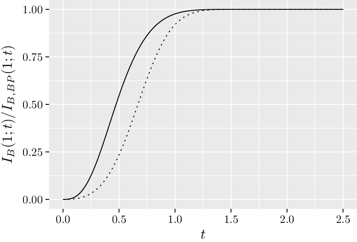
estimators of the the measures $I_\textrm{B}$ and $I_\textrm{B,\,BP}$ can be derived using the MLEs and the representations in Theorems 1 and 2 (cf. Eq. (19)). In Fig. 4, both measures are displayed. We observe that, as mentioned before, $I_\textrm{B}$ lies above $I_\textrm{B,\,BP}$ , and that the limiting behavior is identical in this case.

Figure 4:

Plots of importance measures $I_\textrm{B}(1;\ t)$ (solid) and $I_\textrm{B,\,BP}(1;\ t)$ (dotted) of component 1 for the parallel system with failure-dependent lifetimes based on the Weibull distribution from Example 5.