1. Introduction
Research on bipedal robots has been conducted for decades, and recent advances in computing and artificial intelligence have accelerated progress in this field. While quadrupedal robots have also been widely studied, bipedal robots offer the distinct advantage of potentially serving as substitutes for humans in various tasks and environments [Reference Krishna, Castillo, Mishra, Hereid and Kolathaya1–Reference Dan, Saha and Krishna8]. Their ability to navigate human-accessible spaces makes them an exceptionally versatile form of mobility. However, bipedal robots are still under development, and fully functional humanoid robots capable of seamlessly replacing humans in complex tasks have not yet been realized. This makes the field a challenging yet rewarding area of research.
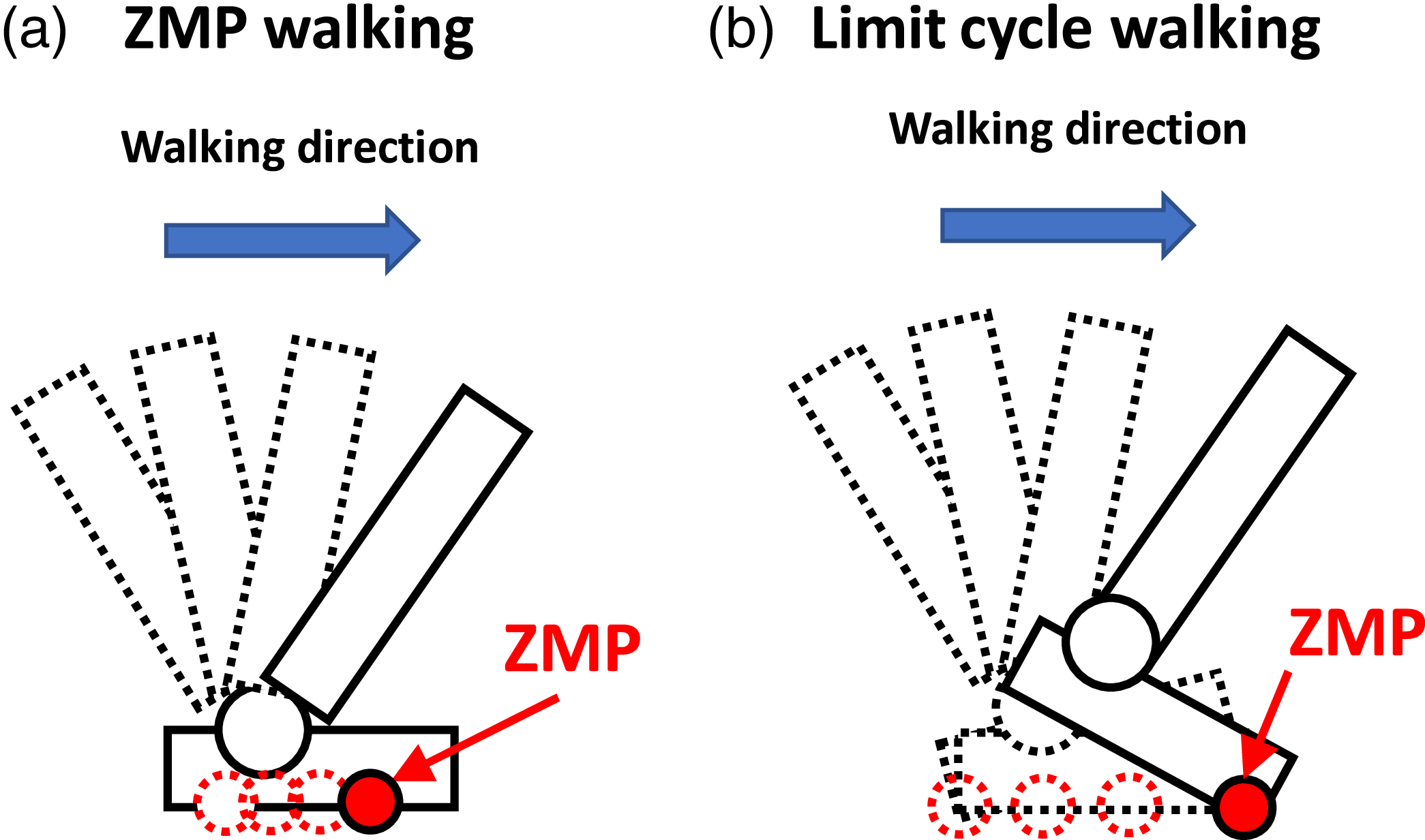
We primarily focused on developing gait generation methods that enable bipedal robots to achieve high-speed locomotion with superior energy efficiency while maintaining balance and preventing falls. Traditionally, zero-moment point (ZMP)-based walking has been the dominant approach for generating stable gaits in bipedal robots [Reference Kajita, Kanehiro, Kaneko, Fujiwara, Harada, Yokoi and Hirukawa9–Reference Shigemi, Goswami and Vadakkepat11]. Moreover, advances in computational power and learning algorithms have led to a growing number of studies employing machine learning to achieve robotic walking. As a result, many robots capable of walking or running have been developed [Reference Rodriguez and Behnke12–Reference Li, Peng, Abbeel, Levine, Berseth and Sreenath16]. However, a key issue from the perspective of safety is the lack of mathematical justification for why such learned walking behaviors are stable and prevent the robot from falling. Limit cycle-based walking methods have emerged as a promising alternative, offering the potential for more natural, human-like walking patterns with enhanced energy efficiency. ZMP-based walking control has been widely adopted for its stability guarantees. Classical ZMP-based methods using the linear inverted pendulum (LIP) model impose the constraint that the ZMP must remain within the support polygon, which restricts the robot’s motion during walking. Under the simplest LIP formulation with constant center of mass height, this constraint prohibits heel-strike and toe-off movements characteristic of human walking, requiring the entire foot to maintain contact with the ground as shown in Figure 1. Several extensions have been proposed to overcome these limitations while maintaining the ZMP framework. The variable height linear inverted Pendulum (VHLIP) model allows height variation of the center of mass, enabling more natural trajectories while still utilizing ZMP constraints. The capture point (CP) concept [Reference Pratt, Carff, Drakunov and Goswami17, Reference Koolen, De Boer, Rebula, Goswami and Pratt18] and its extensions provide systematic methods for stability analysis and recovery. Additionally, approaches incorporating nonlinear dynamics and considering CoP (ZMP) constraints have been developed to achieve more natural motion [Reference Herzog, Rotella, Mason, Grimminger, Schaal and Righetti19].
Variations in ground contact while walking.

Limit cycle-based walking does not impose the ZMP constraint and allows for more dynamic, underactuated behaviors such as heel-strike and toe-off, potentially leading to more efficient and natural gaits. While ZMP-based walking guarantees robust stability by explicitly maintaining the ZMP within the support polygon, limit cycle-based walking achieves stability by treating the walking motion as a stable limit cycle [Reference Collins, Ruina, Tedrake and Wisse20, Reference Hobbelen and Wisse21]. Feedback control is then employed to drive the robot’s state toward a predesigned periodic orbit. Although limit cycle-based walking does not guarantee stability under all conditions, it provides robustness against disturbances within the basin of attraction of the limit cycle. The ability to handle point contact walking itself is not novel. For example, the method in [Reference Herzog, Rotella, Mason, Grimminger, Schaal and Righetti19] employs hierarchical inverse dynamics to optimize joint accelerations and contact forces for momentum-based balance control, achieving stable and robust walking with planar feet. Since the formulation handles generalized contact forces, it could potentially be applied to point contacts with appropriate constraints. However, this method does not consider energy consumption and primarily aims to ensure stability and robustness. In contrast, our method can optimize energy consumption during walking online within a practical control cycle by minimizing control torques while ensuring stability as constraints.
Our proposed approach employs nonlinearmodel predictive control (NMPC) to determine joint torques online by minimizing the tracking error to the desired trajectory and the norm of joint torques during walking. The desired trajectory for energy-efficient walking can be designed offline in advance through optimization of Bézier polynomial coefficients. Although we do not perform this offline optimization in this paper, we demonstrate that such optimization is feasible using existing frameworks that explicitly consider limit cycle stability, such as [Reference Westervelt, Grizzle and Koditschek22]. This separation enables the robot to track the offline-designed energy-efficient trajectory while adapting to disturbances through predictive re-optimization, achieving efficient online computation (0.32 ms per cycle). As demonstrated by the simulations presented in this paper, this approach achieves energy-efficient walking with disturbance recovery capability without sacrificing computational efficiency.
Significant progress has been made in limit cycle-based walking methods, particularly those employing output zeroing control (OZC) through input–output linearization. Several research groups, including Grizzle’s team, have utilized OZC to enhance convergence toward a predefined periodic orbit to achieve energy-efficient active walking [Reference Westervelt, Grizzle and Koditschek22–Reference Gong and Grizzle26]. Other groups have similarly applied this approach to realize stable limit cycle-based walking and running [Reference Selim, Alcı and Altıntas2, Reference Shimizu, Nakaura and Sampei27–Reference Ghansah, Kim, Li and Ames34]. Furthermore, in addition to OZC, both MABEL [Reference Grizzle, Hurst, Morris, Park and Sreenath24] and ATRIAS [Reference Hubicki, Grimes, Jones, Renjewski, Spröwitz, Abate and Hurst30] improve energy efficiency of walking by incorporating large springs at the joints. These robots utilize target trajectories optimized to exploit their mechanical springs for energy-efficient walking, demonstrating effective utilization of the robots’ passive dynamics. In this paper, we use the term ”passive dynamics” to refer to the natural motion that emerges from the mechanical system without active control, which is determined by the system’s inertia, gravity, and mechanical constraints. While the model used in this study does not incorporate springs for simplicity, the proposed approach is extensible to robots with elastic elements. Our proposed framework can optimize trajectories that leverage passive dynamics for improved energy efficiency, similar to these platforms. A key advantage of the NMPC-based approach proposed in this paper is its ability to maintain optimality even when the robot deviates from the desired trajectory. In typical OZC-based control, feedback linearization is employed to track a precomputed desired trajectory, whereas NMPC continuously re-optimizes the control input to guide the robot back to the desired trajectory while considering the full nonlinear dynamics.
OZC approach enables accurate tracking of a predesigned optimal trajectory under ideal conditions, resulting in energy-efficient walking. However, this method inherently relies on high-gain feedback to forcefully eliminate tracking errors without fully leveraging the robot’s dynamics. In real-world environments, various disturbances such as uneven terrain, surface friction variations, motor backlash, and unexpected environmental contacts are inevitable. When such disturbances cause deviations from the desired trajectory, OZC tends to aggressively reconverge using high-gain control, which can result in excessive actuator torques, unwanted oscillations, and ultimately increased energy consumption and reduced stability. These limitations highlight the need for more practical control strategies that actively utilize the robot’s dynamics and can respond to disturbances in a more flexible and energy-efficient manner. To address these challenges, we hypothesized that leveraging the robot’s passive dynamics, similar to the concept of passive dynamic walking introduced by McGeer [Reference McGeer35], could enable the generation of limit cycles with higher energy efficiency. By incorporating the robot’s passive dynamics into the control strategy design, we aim to minimize energy losses caused by external disturbances and achieve more energy-efficient walking. Motivated by this idea, we previously proposed a gait generation method using NMPC to generate limit cycles [Reference Hanazawa, Nishinami and Sagara36]. This method uses NMPC to drive the robot’s state toward a predesigned desired trajectory. NMPC predicts the robot’s future states based on its current state and computes optimal control inputs by solving the optimization problem in real time.
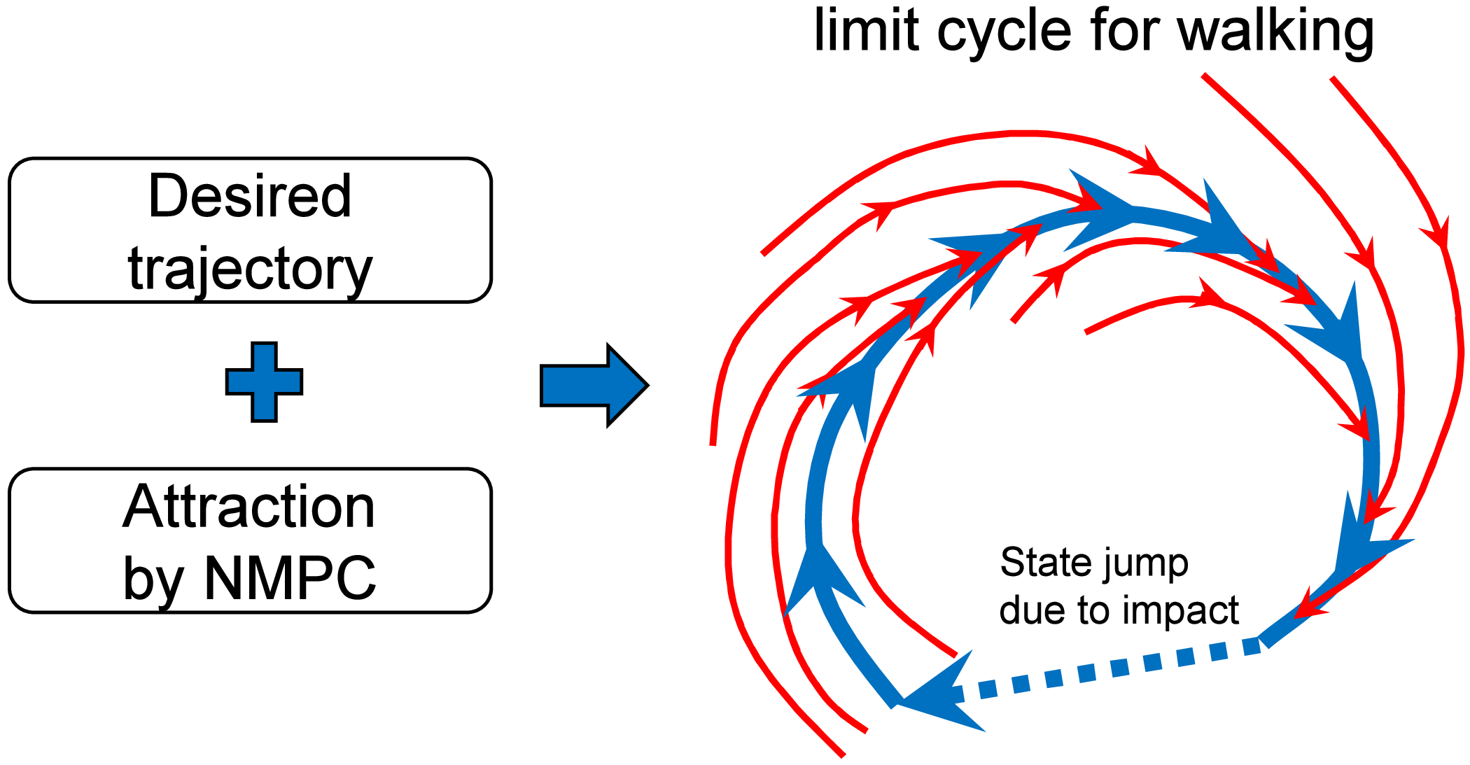
The previously discussed concept of passive dynamic walking realizes energy-efficient locomotion by leveraging the nonlinear passive dynamics arising from the robot’s mechanical structure and the gravitational field on a slope, thereby generating a stable limit cycle. In contrast, NMPC explicitly incorporates the nonlinear dynamics of the robot into a mathematical model, predicts its future behavior, and optimizes the control inputs to achieve convergence to a desired trajectory while minimizing energy consumption. In other words, whereas passive dynamic walking forms a limit cycle by utilizing external gravitational forces, NMPC aims to achieve similar natural dynamic behavior by applying only the minimal necessary actuation, thereby generating a limit cycle in a controlled manner. We have previously hypothesized that the NMPC-based approach can achieve energy-efficient walking similar to passive locomotion, even on level ground. This optimization considers the robot’s dynamics and aims to minimize energy consumption while guiding the robot’s state toward the desired trajectory, as illustrated in Figure 2. Although NMPC entails relatively high computational costs, recent advancements in algorithms for solving NMPC more efficiently [Reference Ohtsuka37, Reference Deng and Ohtsuka38], coupled with the increasing performance of processors, suggest that its implementation on microcontroller-level systems will likely become feasible in the near future.
Limit cycle generation for biped walking.

In our previous work, we applied this method to a rimless wheel-type walking robot, a simplified model of bipedal locomotion, and demonstrated its effectiveness through numerical simulations. The results showed improved the energy efficiency of walking under ideal conditions, with particularly significant improvements observed when walking in disturbed environments [Reference Hanazawa, Nishinami and Sagara36]. However, since our ultimate goal is to achieve energy-efficient locomotion in general humanoid robots, the proposed method must be applicable to biped robots with a higher number of degrees of freedom (DoF). In typical multi-DoF bipedal robots, there exist large and rapid swing leg motions such as thigh swinging and knee bending that were not considered in the rimless wheel model. To enable future analytical optimization of limit cycle trajectories using hybrid zero dynamics (HZD) [Reference Westervelt, Grizzle and Koditschek22], it is essential that all robot states, including swing leg motions, converge strictly to the desired trajectories. Therefore, we aim to develop a control law for biped robots that includes swing leg dynamics and verify whether this control law can achieve both high energy efficiency and strict convergence to the desired walking trajectories.
In this study, we develop limit cycle walking control using NMPC that can be applied to a general and complex bipedal robot model, specifically a five-link robot with sagittal constraints. Numerical simulations were conducted to verify the effectiveness of the proposed method in generating energy-efficient and stable walking with high convergence to the desired trajectory. Furthermore, we implemented the proposed NMPC controller in C language (MEX on MATLAB) to evaluate its computational cost and demonstrate the feasibility of achieving real-time control within the constraints of a typical robot control cycle. The main contributions of this paper are as follows:
-
• Extended the NMPC-based walking control originally proposed for a simplified model [Reference Hanazawa, Nishinami and Sagara36] to a five-link robot by introducing virtual time parameterization within the prediction horizon. This novel extension enables the use of virtual constraints in the NMPC framework, demonstrating that the trajectory optimization framework of conventional HZD can be effectively integrated with NMPC.
-
• Demonstrated that the NMPC-based approach enables online re-optimization of control inputs considering full nonlinear dynamics, allowing the robot to maintain energy efficiency even when deviating from the desired trajectory due to disturbances or model uncertainties, unlike conventional HZD-based methods that rely on offline-optimized trajectories.
-
• Confirmed through numerical simulations that the proposed method generates motions satisfying virtual constraints, validating the integration of HZD and NMPC frameworks for the five-link robot model.
-
• Measured the computation time of the proposed method (0.32 ms per cycle), confirming its feasibility for real-time implementation within typical high-speed control cycles (1 ms), despite being approximately 12 times slower than conventional OZC (0.026 ms per cycle) due to online optimization.
The remainder of this paper is organized as follows: Section 2 introduces the dynamic model of the five-link bipedal robot. Section 3 details the proposed NMPC-based controller. Section 4 presents the results of our walking analysis and demonstrates the effectiveness of the proposed method through numerical simulations. Finally, Section 5 provides concluding remarks and discusses potential directions for future research.
2. Modeling of the five-link bipedal robot
2.1. Equation of motion
We use a model of a five-link biped robot (Figure 3). Although we aim to apply our method to robots with flat feet, such as the illustrated in Figure 1, in future work, this paper focuses on a simplified case. Specifically, we consider a robot with point-contact feet that remain underactuated at all times. Figure 4 illustrates the details of the torques exerted by each motor between the links. The red arrows represent the torques generated by the motors, while the purple arrows indicate the reaction torques corresponding to those motor outputs. This robot also has four actuators for active control and its torso is equipped with a 9-axis sensor, which allows measurement of its orientation and angular velocity in the absolute coordinate frame. Each joint is equipped with an encoder that measures the relative joint angle between connected links. Angular velocities can then be obtained by differentiating these angle measurements. Therefore, we assume that the full state of the robot is observable. In this study, we derive the equations of motion using the Euler–Lagrange method, which is widely used in general applications. Equation of motion of the robot is given by
 \begin{equation} \boldsymbol{M}(\boldsymbol{q})\ddot {\boldsymbol{q}}+\boldsymbol{H}(\boldsymbol{q},\dot {\boldsymbol{q}})=\boldsymbol{S}\boldsymbol{u}, \end{equation}
where
 $\boldsymbol{q}=[\theta _{1},\,\theta _{2},\,\theta _{3},\,\theta _{4},\,\theta _{5}]^{\mathrm{T}}$
is the generalized coordinate vector,
 $\boldsymbol{M}(\boldsymbol{q})\in \mathbb{R}^{5\times 5}$
is the inertia matrix,
 $\boldsymbol{H}(\boldsymbol{q},\dot {\boldsymbol{q}})\in \mathbb{R}^{5}$
is the vector that consists of Coriolis, centrifugal forces, as well as the gravitational vector,
 $\boldsymbol{u} = [u_{1},\,u_{2},\,u_{3},\,u_{4}]^{\mathrm{T}}$
is the input torque vector, and
 $\boldsymbol{S} \in \mathbb{R}^{5\times 4}$
is the driving matrix, which is expressed as:
 \begin{equation*} \boldsymbol{S}=\left [ \begin{array}{c@{\quad}c@{\quad}c@{\quad}c} -1 & 0 & 0 & 0 \\[2pt] 1 & 0 & 0 & -1 \\[2pt] 0& 1 & -1 & 0 \\[2pt] 0 & 0 & 1 & 0\\[2pt] 0 & -1 & 0 & 1 \end{array} \right ]. \end{equation*}
Five-link biped model.

Details of the torques acting on the robot (the red arrows indicate the torques generated by the motors, while the purple arrows represent the reaction torques against the motor torques.).

The details of the equation of motion are provided in the Appendix.
2.2. Impact equation
The walking motion of a bipedal robot involves collision phenomena between the swing leg and the ground during locomotion, requiring the modeling of this behavior. To address this, a collision equation is introduced to compute the generalized velocities immediately after the collision, based on the robot’s state immediately prior to impact. It is assumed that the collision between the swing leg and the ground is perfectly inelastic and instantaneous. At the moment of collision, velocity constraints arise in both the horizontal and vertical directions at the end of swing leg. These relationships can be expressed as follows:
 \begin{align*} l_1\cos \theta _1 \dot {\theta }_1 +l_2\cos \theta _2 \dot {\theta }_2 - l_2\cos \theta _3 \dot {\theta }_3 + l_1\cos \theta _4 \dot {\theta }_4 + \,\,\dot \!\!{x}_1 &= 0, \\[3pt] -l_1\sin \theta _1 \dot {\theta }_1 - l_2\sin \theta _2\dot {\theta }_2 + l_2\sin \theta _3\dot {\theta }_3 + l_1\sin \theta _4 \dot {\theta }_4 + \dot {z}_1 &= 0, \end{align*}
where
 $\,\,\dot \!\!{x}_{1}$
and
 $\dot {z}_{1}$
represent the velocities of the support leg’s end in the horizontal and vertical directions, respectively. From the these equations, the instantaneous constraint Jacobian matrix at the moment of collision,
 $\boldsymbol{J}_I(\boldsymbol{q}_a) \in \mathbb{R}^{2 \times 7}$
, is derived as follows:
 \begin{eqnarray*} \boldsymbol{J}_{I}(\boldsymbol{q}_a)=\left [ \begin{array}{c@{\quad}c@{\quad}c@{\quad}c@{\quad}c@{\quad}c@{\quad}c} l_1 C_1 & l_2 C_2 & -l_2 C_3 & -l_1 C_4 & 0 & 1 & 0 \\[3pt] -l_1 S_1 & -l_2 S_2 & l_2 S_3 & l_1S_4 & 0 & 0 & 1 \\ \end{array} \right ], \end{eqnarray*}
where
 $C_i$
is the
 $\cos \theta _i$
and
 $S_i$
is the
 $\sin \theta _i$
. At this moment, the impulse vector
 $\boldsymbol{\lambda }_I \in \mathbb{R}^{2}$
generated during the collision and the generalized velocity of the robot immediately after the collision,
 $\dot {\boldsymbol{q}_{\boldsymbol{a}}^{\boldsymbol{+}}} \in \mathbb{R}^7$
, can be obtained as follows:
 \begin{align} \boldsymbol{\lambda }_{I} &=-\boldsymbol{X}_{I}(\boldsymbol{q}_a)^{-1}\boldsymbol{J}_{I}(\boldsymbol{q_a})\dot {\boldsymbol{q}}_a^{-}, \\[-10pt]\nonumber\end{align}
 \begin{align} \boldsymbol{X}_{I}({\boldsymbol{q}}_a) &=\boldsymbol{J}_{I}({\boldsymbol{q}_a})\boldsymbol{M}_{a}(\boldsymbol{q}_a)^{-1}\boldsymbol{J}_{I}(\boldsymbol{q}_a)^{\mathrm{T}}, \\[-10pt]\nonumber\end{align}
 \begin{align} \dot {\boldsymbol{q}}_a^{+} &=(\boldsymbol{I}-\boldsymbol{M}_{a}(\boldsymbol{q}_a)^{-1}\boldsymbol{J}_{I}(\boldsymbol{q}_a)^{\mathrm{T}}\boldsymbol{X}_{I}(\boldsymbol{q}_a)^{-1}\boldsymbol{J}_{I}(\boldsymbol{q}_a))\dot {\boldsymbol{q}}_a^{-}, \end{align}
where
 $\boldsymbol{q}_a =[\theta _{1},\,\theta _{2},\,\theta _{3},\,\theta _{4},\,\theta _{5},\,x_1,\,z_1]^{\mathrm{T}}$
is the generalized coordinate vector in the augmented equation of motion and
 $\boldsymbol{M}_{a}(\boldsymbol{q}_a) \in \mathbb{R}^{7\times 7}$
represents the inertia matrix derived from the augmented equation of motion for the free-falling robot, incorporating the generalized coordinates and the coordinate components
 $x_1$
and
 $z_1$
of the support leg’s end. Additionally,
 $\dot {\boldsymbol{q}_{\boldsymbol{a}}^{\boldsymbol{-}}} \in \mathbb{R}^7$
denotes the velocity vector immediately before the collision. Finally, the angular velocity obtained from Eq. (4) is used to update the robot’s state vector to reflect its post-collision condition. The detailed derivation of the impact equations can be found in the literature by Grizzle et al. [Reference Grizzle, Abba and Plestan23].
3. NMPC design for limit cycle walking
3.1. Overview of NMPC for biped robots
In this paper, we construct NMPC for realizing walking motion of a five-link robot by incorporating several improvements based on the NMPC previously implemented on rimless wheels [Reference Hanazawa, Nishinami and Sagara36]. Figure 5 shows a schematic diagram of the control flow using the proposed method in this paper. The parts that significantly differ from prior research are indicated by yellow blocks. The main improvements over existing methods are the following three points. At the control steps immediately after gait initiation and stance leg exchange, the robot state changes discontinuously, and thus the control input by C/GMRES-based NMPC cannot be derived. Therefore, a separate input to mitigate the impact effect is employed at these steps. Second, we set the prediction horizon as a function dependent on virtual time. This is because the tracking performance to the desired trajectory of the swing leg motion, which changes rapidly during walking, was insufficient. Therefore, we resolve this issue by varying the prediction horizon according to virtual time. Finally, although not shown in this figure, we set the desired trajectory as a function dependent on virtual time and also modify the desired trajectory within the prediction by considering this virtual time. These details are presented below.
Control flow of the proposed NMPC: the yellow blocks represent the elements that were newly added in this paper to prevent divergence of the NMPC.

3.2. Discrete-time NMPC
This section describes the discrete-time NMPC applied to a biped walking robot. The discrete-time nonlinear system is defined as follows:
 \begin{align} \boldsymbol{x}_{i+1}(t) &=\boldsymbol{x}_{i}(t) + \boldsymbol{f}(\boldsymbol{x}_{i}(t), \boldsymbol{u}_{i}(t))\Delta \tau , \\[-8pt]\nonumber\end{align}
 \begin{align} \boldsymbol{x}_{0}(t)&=\boldsymbol{x}(t), \end{align}
where
 $i=0, \ldots , N-1$
,
 $N$
is the number of prediction steps,
 $\Delta \tau = T/N$
is the discrete interval of the prediction horizon,
 $T$
is the prediction horizon, and
 $\boldsymbol{x}_i(t)\in {\mathbb R}^{n}$
and
 $\boldsymbol{u}_i(t) \in {\mathbb R}^{m}$
are the state and input vectors at
 $i$
-th step of the prediction horizon at time
 $t$
, respectively. The objective function is defined as:
 \begin{equation} J \,:\!=\, \varphi (\boldsymbol{x}_N(t)) + \Sigma ^{N-1}_{i=0}L(\boldsymbol{x}_i(t),\boldsymbol{u}_i(t))\Delta \tau , \end{equation}
where
 \begin{align} \varphi (\boldsymbol{x}_N(t))&=\frac {1}{2}(\boldsymbol{x}_{N}(t)-\boldsymbol{x}_{d, N}(t))^{\mathrm{T}}\boldsymbol{S}_f(\boldsymbol{x}_{N}(t)-\boldsymbol{x}_{d,N}(t)), \\[-8pt]\nonumber\end{align}
 \begin{align} L&=\frac {1}{2}(\boldsymbol{x}_{i}(t)-\boldsymbol{x}_{d,i}(t))^{\mathrm{T}}\boldsymbol{Q}(\boldsymbol{x}_{i}(t)-\boldsymbol{x}_{d,i}(t)) + \boldsymbol{u}^{\mathrm{T}}_{i}(t)\boldsymbol{R}\boldsymbol{u}_{i}(t), \end{align}
 $\boldsymbol{x}_{d,i}$
is the desired state vector at
 $i$
-th step of the prediction horizon,
 $\boldsymbol{S}_f$
is the weight for the terminal cost,
 $\boldsymbol{Q}$
is the weight for the stage cost of the state, and
 $\boldsymbol{R}$
is the weight for the stage cost of the input. Then, the Hamiltonian and necessary conditions for optimality are given obtained as:
 \begin{align} H(\boldsymbol{x}_i(t),\boldsymbol{u}_i(t),\boldsymbol{\lambda }_{i+1}(t)) \,:\!=\, L + \boldsymbol{\lambda }^{\mathrm{T}}_{i+1}(t)\,\boldsymbol{f}(\boldsymbol{x}_{i}(t),\boldsymbol{u}_{i}(t)), \\[-10pt]\nonumber\end{align}
 \begin{align} \boldsymbol{\lambda }_N(t) =\frac {\partial \varphi ^{\mathrm{T}}}{\partial \boldsymbol{x}}(\boldsymbol{x}_N(t)), \\[-10pt]\nonumber\end{align}
 \begin{align} \boldsymbol{\lambda }_i(t) = \boldsymbol{\lambda }_{i+1}(t) + \frac {\partial H^{\mathrm{T}}}{\partial \boldsymbol{x}}(\boldsymbol{x}_i(t),\boldsymbol{u}_i(t),\boldsymbol{\lambda }_{i+1}(t))\Delta \tau , \\[-10pt]\nonumber\end{align}
 \begin{align} \frac {\partial H}{\partial \boldsymbol{u}}(\boldsymbol{x}_i(t),\boldsymbol{u}_i(t),\boldsymbol{\lambda }_{i+1}(t)) = 0, \end{align}
where
 $\boldsymbol{\lambda }_i(t) \in {\mathbb R}^{n}$
represents the adjoint (co-state) variable vector at
 $i$
-th step. The optimal control input at the first step is used as the actual input for the system, followed by a receding of the finite horizon and repeating this sequence. To efficiently solve the NMPC, the C/GMRES method proposed by Ohtsuka [Reference Ohtsuka37] is employed. In this method,
 $\boldsymbol{U}(t)$
and
 $F(\boldsymbol{U}(t), \boldsymbol{x}(t), t)$
are defined as:
 \begin{align} \boldsymbol{U}(t) &\,:\!=\, [u_0^{\mathrm{T}}(t), \ldots ,u_{N-1}^{\mathrm{T}}(t)]^{\mathrm{T}}, \\[-10pt]\nonumber\end{align}
 \begin{align} \boldsymbol{F}(\boldsymbol{U}(t),\boldsymbol{x}(t),t) &\,:\!=\, \left [ \begin{array}{c} \boldsymbol{H}_u^{\mathrm{T}}(\boldsymbol{x}_0(t),\boldsymbol{u}_0(t),\boldsymbol{\lambda _1}(t)),\\ \vdots \\ \boldsymbol{H}_u^{\mathrm{T}}(\boldsymbol{x}_{N-1}(t),\boldsymbol{u}_{N-1}(t),\boldsymbol{\lambda }_N(t)), \end{array} \right ], \end{align}
where
 $H_u = \frac {\partial H}{\partial u}$
. Subsequently, Eq. (10)–(13) are used to compute the state and adjoint variable vectors. By solving
 $\boldsymbol{F}=0$
with the C/GMRES algorithm,
 $\dot {\boldsymbol{U}}(t)$
is obtained.
3.3. Extension of NMPC considering robustness
To enhance robustness against modeling errors in NMPC and improve the stability of inputs when discrete state and input jumps occur, an augmented system is constructed by incorporating the input derivative
 $\dot {\boldsymbol{u}}$
as a new state. This approach, as proposed by Onodera et al. and Murayama et al. [Reference Onodera and Yamakita39, Reference Murayama and Yamakita40], treats the input as part of the state. Two types of discrete jumps must be considered: (a) jumps induced by minor collisions during walking (excluding swing leg collisions that trigger stance leg switching) and (b) jumps resulting from the control strategy in our approach, where the control input immediately after stance leg switching is designed to cancel the impact in the first step, followed by a transition to NMPC in subsequent steps. In both scenarios, the state–input relationship undergoes rapid changes, which can cause instability and potential divergence in NMPC. The incorporation of an integrator into the augmented system improves the numerical stability of NMPC even under these discrete jumps, thereby preventing optimization divergence and facilitating smoother walking motion.
The augmented system, which includes the input as a state for the five-link walking robot considered in this study, is expressed as:
 \begin{align} \boldsymbol{x}(i+1)= \left [ \begin{array}{c} y_1(i+1)\\[2pt] y_2(i+1)\\[2pt] y_3(i+1)\\[2pt] y_4(i+1)\\[2pt] y_5(i+1)\\[2pt] y_6(i+1)\\[2pt] y_7(i+1)\\[2pt] y_8(i+1)\\[2pt] y_9(i+1)\\[2pt] y_{10}(i+1)\\[2pt] u_1(i+1)\\[2pt] u_2(i+1)\\[2pt] u_3(i+1)\\[2pt] u_4(i+1) \end{array} \right ]&= \left [ \begin{array}{c} y_1(i) + y_6(i)\Delta \tau \\[2pt] y_2(i) + y_7(i)\Delta \tau \\[2pt] y_3(i) + y_8(i)\Delta \tau \\[2pt] y_4(i) + y_9(i)\Delta \tau \\[2pt] y_5(i) + y_{10}(i)\Delta \tau \\[2pt] y_6(i) + \ddot {\theta }_1(i) \Delta \tau \\[2pt] y_7(i) + \ddot {\theta }_2(i) \Delta \tau \\[2pt] y_8(i) + \ddot {\theta }_3(i) \Delta \tau \\[2pt] y_9(i) + \ddot {\theta }_4(i) \Delta \tau \\[2pt] y_{10}(i) + \ddot {\theta }_5(i) \Delta \tau \\[2pt] u_1(i)\\[2pt] u_2(i)\\[2pt] u_3(i)\\[2pt] u_4(i) \end{array} \right ]+ \left [ \begin{array}{c} \boldsymbol{0}_{10 \times 4}\\[2pt] \boldsymbol{D} \end{array} \right ]\dot {\boldsymbol{u}}(i), \nonumber\\[2pt] &=\boldsymbol{f}(\boldsymbol{x}(i)) + \boldsymbol{g}\dot {\boldsymbol{u}}(i), \end{align}
where
 $y_1(i), y_2(i), \ldots , y_5(i)$
are the output angles of the robot’s links,
 $y_6(i), y_7(i), \ldots , y_{10}(i)$
are the output angular velocities of the robot’s links, and
 $\dot {\boldsymbol{u}}(i) = [\dot {u}_{1}(i),\,\dot {u}_{2}(i),\,\dot {u}_{3}(i),\,\dot {u}_{4}(i)]^{\mathrm{T}}$
is the vector of the time derivative of the robot’s inputs at
 $i$
-th step of the prediction horizon.
 $\boldsymbol{D}$
is defined as:
 \begin{align} \boldsymbol{D} = \left [ \begin{array}{c@{\quad}c@{\quad}c@{\quad}c} \Delta \tau & 0 & 0 & 0\\ 0 & \Delta \tau & 0 & 0\\ 0 & 0 & \Delta \tau & 0\\ 0 & 0 & 0 &\Delta \tau \end{array} \right ]. \end{align}
 $\boldsymbol{\ddot {\theta }}(i)=[\ddot {\theta }_{1}(i),\,\ddot {\theta }_{2}(i),\,\ddot {\theta }_{3}(i),\,\ddot {\theta }_{4}(i),\,\ddot {\theta }_{5}(i)]^{\mathrm{T}}$
is the vector of the robot’s angular acceleration at
 $i$
-th step of the prediction horizon given by:
 \begin{equation} \ddot {\boldsymbol{\theta }}(i)= \boldsymbol{M}^{-1}(\boldsymbol{q}(i))(\boldsymbol{S}\boldsymbol{u}(i)-\boldsymbol{H}(\boldsymbol{q}(i),\dot {\boldsymbol{q}}(i))). \end{equation}
In this case, the objective function is defined as:
 \begin{align} J \,:\!=\, \varphi (\boldsymbol{x}(N), \boldsymbol{y}_d(N)) + \Sigma ^{N-1}_{i=0}L(\boldsymbol{x}(i),\dot {\boldsymbol{u}}(i)) \Delta \tau , \end{align}
where
 \begin{align} \varphi (\boldsymbol{x}(N), \boldsymbol{y}_d(N))&=\frac {1}{2}(\boldsymbol{y}(N)-\boldsymbol{y}_{d}(N))^{\mathrm{T}} \boldsymbol{S}_f(\boldsymbol{y}(N)-\boldsymbol{y}_d(N)), \\[-10pt]\nonumber\end{align}
 \begin{align} L(\boldsymbol{x}(i), \dot {\boldsymbol{u}}(i), \boldsymbol{y}_d(i))&=\frac {1}{2}(\boldsymbol{y}(i)-\boldsymbol{y}_{d}(i))^{\mathrm{T}}\boldsymbol{Q}(\boldsymbol{y}(i)-\boldsymbol{y}_{d}(i))\nonumber \\[8pt] &+ \frac {1}{2} \dot {\boldsymbol{u}}(i)^{\mathrm{T}} \boldsymbol{R} \dot {\boldsymbol{u}}(i), \end{align}
 $\boldsymbol{y}_d(i)$
is the vector of the desired output values. The Hamiltonian is defined as:
 \begin{align} H(\boldsymbol{x}(i),\dot {\boldsymbol{u}}(i),\boldsymbol{\lambda }(i+1)) & \,:\!=\, L + \boldsymbol{\lambda }^{\mathrm{T}}(i+1)(\boldsymbol{f}(\boldsymbol{x}(i))+\boldsymbol{g}\dot {\boldsymbol{u}}(i)). \end{align}
From Eq. (23), the necessary conditions for optimality are obtained as follows:
 \begin{align} \frac {\partial H}{\partial \dot {\boldsymbol{u}}}&=\dot {\boldsymbol{u}}^{\mathrm{T}}(i)\boldsymbol{R}+\boldsymbol{\lambda }^{\mathrm{T}}(i+1)\boldsymbol{g}, \end{align}
 \begin{align} &= 0. \end{align}
Therefore, the optimal control input
 $\dot {\boldsymbol{u}}$
can be obtained using C/GMRES, and the input vector
 $\boldsymbol{u}$
to be used in the real system can be obtained by integrating
 $\dot {\boldsymbol{u}}$
.
Up to this point, the proposed method was an extension of our previous control law for a rimless wheel robot to a five-link biped [Reference Hanazawa, Nishinami and Sagara36]. However, this extension alone resulted in stability issues in the NMPC, particularly around the time of the swing leg impact. To address this issue, we further introduced improvements to the control input immediately after the impact (or at the beginning of the walking phase) and to the prediction horizon in the NMPC, as detailed below.
3.4. Nonlinear cancellation input
For the first step at the start of walking and that immediately following a support leg transition, the input is not derived from model predictive control but rather calculated as follows:
 \begin{align} \boldsymbol{u}^{+} = -(L_{g}L_{f}h)^{-1}(L_{f}^2h - \boldsymbol{v}^{+}), \end{align}
where
 $\boldsymbol{v}^{+} = [0,\,0,\,0,\,0]^{\mathrm{T}}$
. Leveraging the robot’s dynamics,
 $L_gL_fh$
and
 $L_{f}^2h$
are determined as follows:
 \begin{align} L_{g}L_{f}h &= \boldsymbol{C}\boldsymbol{M}^{-1}(\boldsymbol{q})\boldsymbol{S}, \\[-10pt]\nonumber\end{align}
 \begin{align} L_{f}^2h &= -\boldsymbol{C}\boldsymbol{M}^{-1}(\boldsymbol{q})\boldsymbol{H}(\boldsymbol{q},\dot {\boldsymbol{q}}), \end{align}
and
 $\boldsymbol{C}$
is given by the following matrix:
 \begin{equation*} \boldsymbol{C}=\left [ \begin{array}{c@{\quad}c@{\quad}c@{\quad}c@{\quad}c} -1 & 1 & 0 & 0 & 0\\[2pt] 0 & -1 & 1 & 0 & 0\\[2pt] 0& 0 & -1 & 1 & 0\\[2pt] 0 & 0 & 0 & 0 & 1 \end{array} \right ]. \end{equation*}
This input is designed solely to cancel out gravitational, centrifugal, Coriolis, and inertial forces and does not contribute to correcting the robot’s state toward the target trajectory. While this is not the optimal input, the control performance should not degrade significantly as long as the robot’s state immediately after the support leg transition remains close to the target trajectory.
3.5. Design of prediction horizon function
In NMPC, it is necessary to set a prediction horizon. In our NMPC, the prediction horizon is defined by the following function:
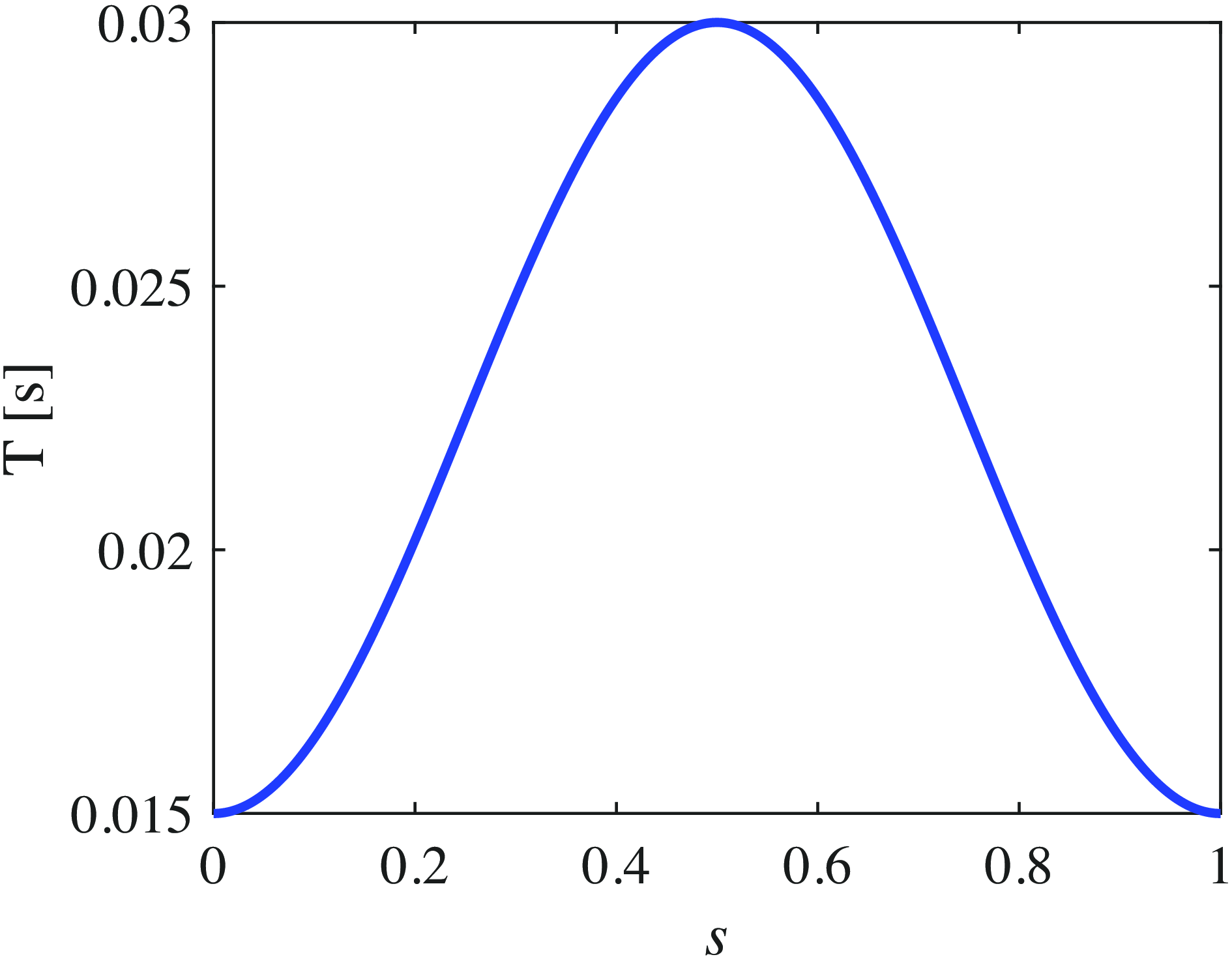
 \begin{equation} T(s) \,=\!:\, T_{\min} + \frac {(T_{\max}-T_{\min})(1-\cos (2\pi s))}{2}, \end{equation}
where
 $T_{\min}$
and
 $T_{\max}$
are the minimum and maximum values of the prediction horizon, respectively. Then,
 $s$
is obtained as:
 \begin{equation} s(\theta _{v})\,:\!=\, \frac {\theta _{v}-\theta ^{+}_{v}}{\theta ^{-}_{v}-\theta ^{+}_{v}}, \end{equation}
Prediction horizon with respect to
 $s(\theta _v)$
at
 $T_{\min} = 0.015$
s and
 $T_{\max} = 0.03$
s.

where
 $\theta _{v} = (\theta _1 + \theta _2) / 2$
is the angle of the virtual support leg, and
 $\theta ^{-}_{v}$
and
 $\theta ^{+}_{v}$
are the angles immediately before and after the swing leg collision (after the support leg exchange), respectively. Here,
 $s$
is referred to as the virtual time, and it is a variable determined by the robot’s state, independent of real time [Reference Westervelt, Grizzle, Chevallereau, Choi and Morris41].
The virtual time,
 $s$
, is 0 immediately after the support leg transition, and it increases monotonically, reaching 1 just before the next support leg transition. Using this function, the prediction horizon changes as shown in Figure 6. Immediately after the support leg transition, the robot’s dynamics change abruptly owing to leg collision; therefore, the prediction horizon should be kept short. However, during the middle of the stance phase, where the dynamics change more gradually, a longer prediction horizon is preferable. In the latter half of the stance phase, where swing leg collisions occur, the prediction horizon should be kept as short as possible. To meet these requirements, a prediction horizon function that depends on this virtual time was designed.
3.6. Design of desired trajectories
Generating a stable limit cycle requires a periodic trajectory for the NMPC to track. This paper introduces a virtual constraint, represented as a Bézier curve, depending on a virtual time, as proposed by Westervelt et al. [Reference Westervelt, Grizzle and Koditschek22, Reference Westervelt, Grizzle, Chevallereau, Choi and Morris41]. The introduction of this virtual constraint ensures that the robot’s motion is realized independently of real time. This approach simplifies the design of optimal trajectories for stable periodic walking. Furthermore, trajectory optimization can be performed within the framework of HZD [Reference Westervelt, Grizzle and Koditschek22]. For simplicity, we did not optimize the virtual constraint trajectory; instead, we determined it through a trial-and-error approach. Controlling the torso angle (
 $\theta _5$
), relative angle of the support leg’s knee joint (
 $\gamma$
), relative angle between the support leg and the swing leg’s hip joints (
 $\phi$
), and angle of the swing leg’s knee joint (
 $\eta$
). The desired relative angle between the support and swing legs,
 $\phi _d(s)$
and that of the swing leg’s knee joint,
 $\eta _d(s)$
, are designed using Bézier curves with the virtual time parameter,
 $s$
, as follows:
 \begin{equation} \phi _{d}(s)\,:\!=\, \sum _{l=0}^{M}\alpha _{l}^{\phi }\frac {M!}{l!(M-l)!}s^{l}(1-s)^{M-l}, \end{equation}
 \begin{equation} \eta _{d}(s)\,:\!=\, \sum _{l=0}^{M}\alpha _{l}^{\eta }\frac {M!}{l!(M-l)!}s^{l}(1-s)^{M-l}, \end{equation}
where
 $\alpha _l^{\phi }$
and
 $\alpha _l^{\eta }(s)$
are the control points that determine
 $\phi _d(s)$
and
 $\eta _d(s)$
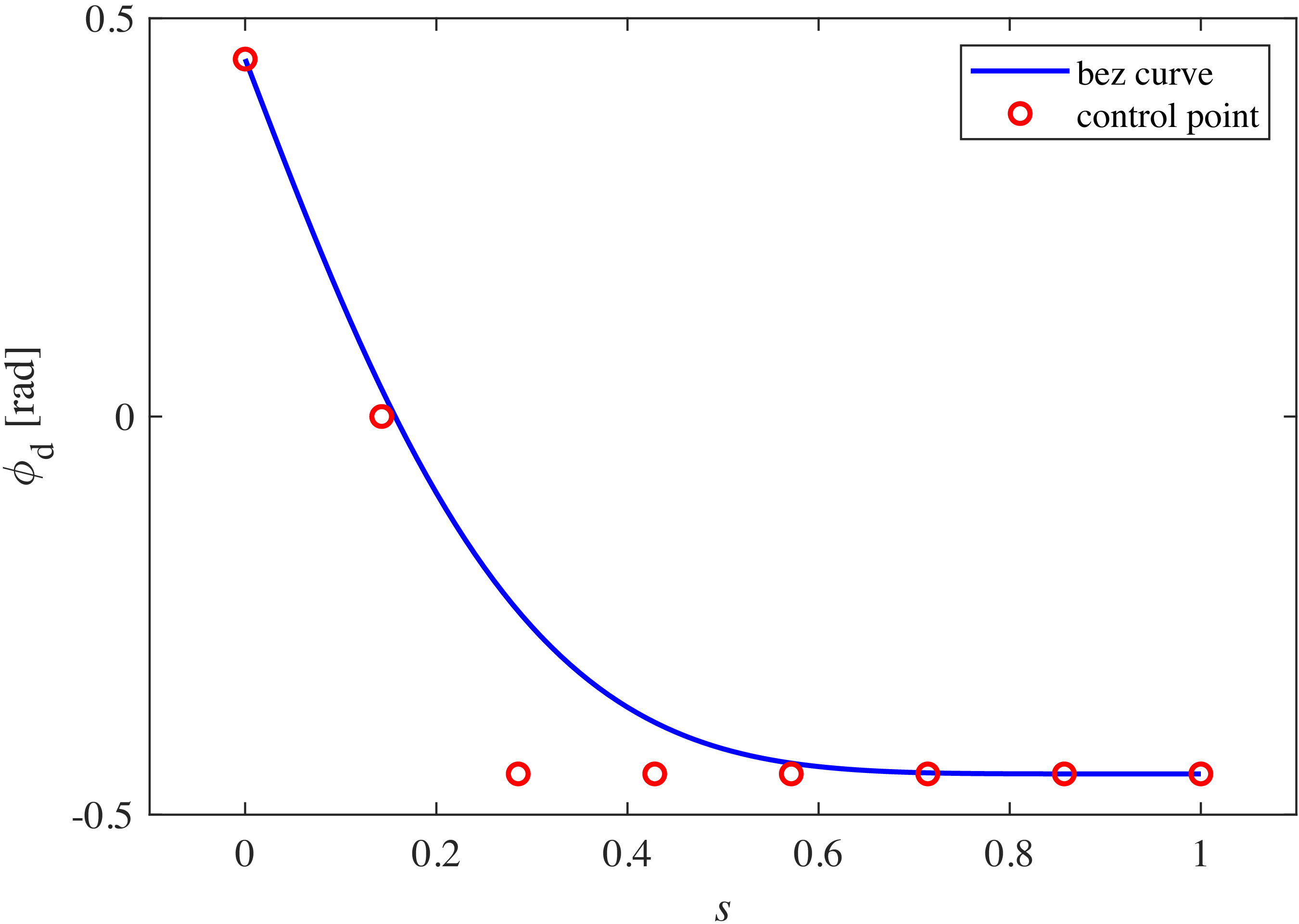
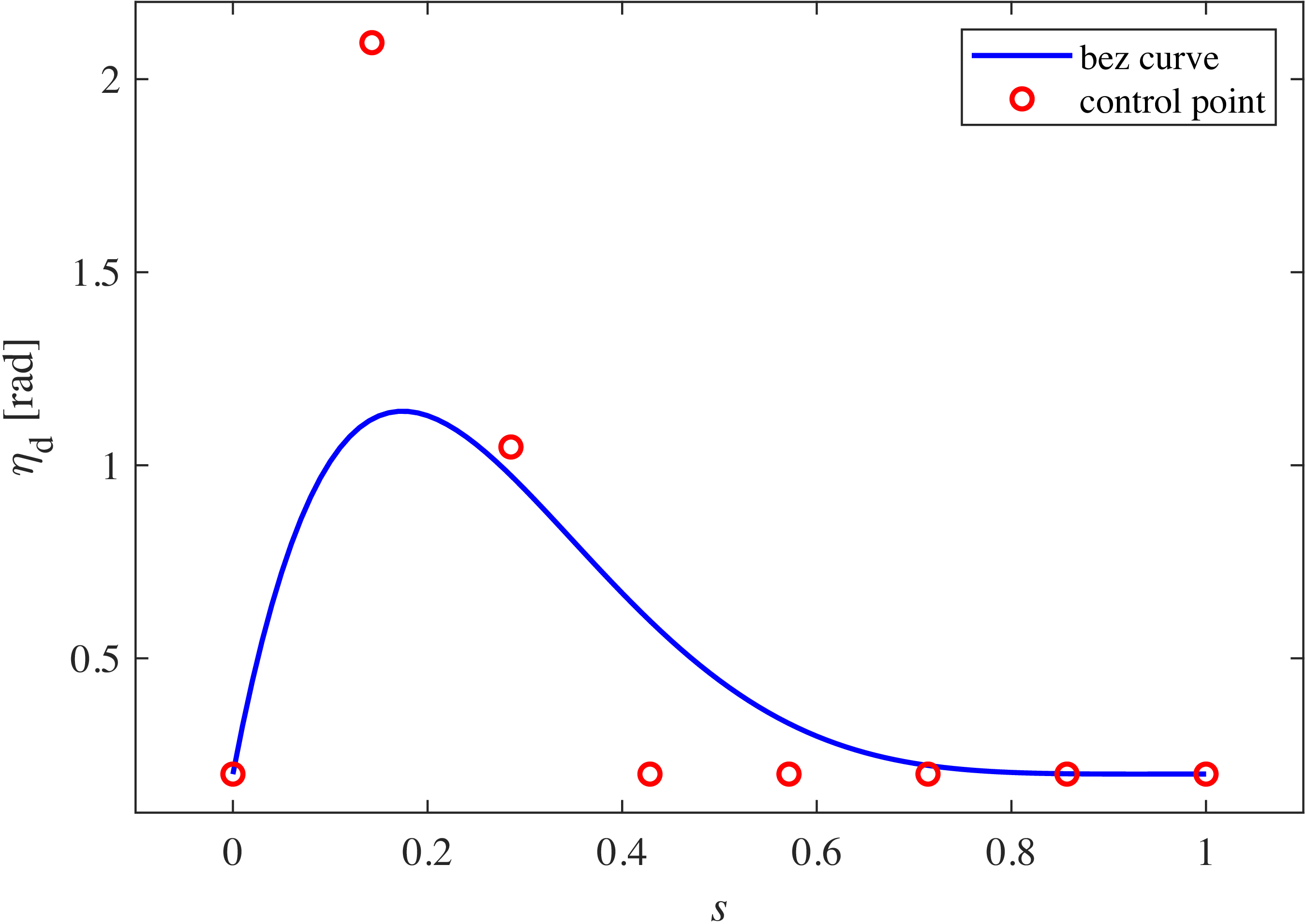
, respectively. The designed Bézier curves are shown in Figures 7 and 8. Moreover, the torso angle was set to
 $\theta _{5d} = 0.05$
rad and the knee angle of the support leg to
 $\gamma _{d} = 0.2$
rad. For simplicity, these two angles were assigned fixed values based on the assumption that they do not vary significantly during walking. However, it is also possible to define their continuous trajectories using Bézier curves. The details of
 $\boldsymbol{y}_{d}(i)$
are then obtained as follows:
 \begin{align} \boldsymbol{y}_{d}(i)= \left [ \begin{array}{c} 0 \\[6pt] y_1(i) - \gamma _{d} \\[6pt] y_2(i) + \phi _{d}(s) \\[6pt] y_3(i) + \eta _{d}(s) \\[6pt] \theta _{5d} \\[6pt] 0 \\[6pt] y_6(i) \\[10pt] y_7(i) + \dfrac {\partial \phi _d(s)}{\partial s}\dfrac {\partial s}{\partial \theta _v}\dfrac {\partial \theta _v}{\partial t}\\[18pt] y_8(i) + \dfrac {\partial \eta _d(s)}{\partial s}\dfrac {\partial s}{\partial \theta _v}\dfrac {\partial \theta _v}{\partial t}\\[10pt] 0 \end{array} \right ]. \end{align}
Desired trajectory of the thigh of swing leg at
 $\alpha _{0}^{\phi }=\pi /7$
,
 $\alpha _{1}^{\phi }=0$
,
 $\alpha _{2}^{\phi }=-\pi /7$
,
 $\alpha _{3}^{\phi }=-\pi /7$
,
 $\alpha _{4}^{\phi }=-\pi /7$
,
 $\alpha _{5}^{\phi }=-\pi /7$
,
 $\alpha _{6}^{\phi }=-\pi /7$
, and
 $\alpha _{7}^{\phi }=-\pi /7$
.

4. Walking analysis
To demonstrate the effectiveness of the proposed method, its walking performance is compared with that of a conventional OZC approach through numerical simulations.
Desired trajectory of the knee of swing leg at
 $\alpha _{0}^{\eta }=0.2$
,
 $\alpha _{1}^{\eta }=\pi /1.5$
,
 $\alpha _{2}^{\eta }=-\pi /3$
,
 $\alpha _{3}^{\eta }=0.2$
,
 $\alpha _{4}^{\eta }=0.2$
,
 $\alpha _{5}^{\eta }=0.2$
,
 $\alpha _{6}^{\eta }=0.2$
, and
 $\alpha _{7}^{\eta }=0.2$
.

4.1. Details of analysis
4.1.1. OZC
First, we briefly explain the OZC method employed in this study. The inputs and outputs are linearized, and the input obtained via proportional-derivative control is used as the new input. The input required for output zeroing is given by:
 \begin{align} \boldsymbol{u} = -(L_{g}L_{f}h)^{-1}(L_{f}^2h - \boldsymbol{v}), \end{align}
where
 $\boldsymbol{v} = [v_{1},\,v_{2},\,v_{3},\,v_{4}]^{\mathrm{T}}$
is the new input vector. The elements of
 $\boldsymbol{v}$
are then obtained as follows:
 \begin{align} v_{1} &= -K_{P1}(\theta _2-\theta _1+\gamma _d)-K_{D1}(\dot {\theta }_2-\dot {\theta }_{1}), \\[-10pt]\nonumber\end{align}
 \begin{align} v_{2} &= -K_{P2}(\theta _3-\theta _2+\phi _{d}(s))-K_{D2}\left(\dot {\theta }_3-\dot {\theta }_2+\frac {\partial \phi _d (s)}{\partial s}\frac {\partial s}{\partial \theta _v}\frac {\partial \theta _v}{\partial t}\right), \\[-5pt]\nonumber\end{align}
 \begin{align} v_{3} &= -K_{P3}(\theta _4-\theta _3-\eta _{d}(s))-K_{D3}\left(\dot {\theta }_4-\dot {\theta }_3-\frac {\partial \eta _d (s)}{\partial s}\frac {\partial s}{\partial \theta _v}\frac {\partial \theta _v}{\partial t}\right), \\[-5pt]\nonumber\end{align}
 \begin{align} v_{4} &= -K_{P4}(\theta _5-\theta _{5d})-K_{D4}\dot {\theta }_5. \end{align}
The gains were set as
 $K_{P1} = 6000$
,
 $K_{D1} = 600$
,
 $K_{P2} = 8000$
,
 $K_{D2} = 800$
,
 $K_{P3} = 8000$
,
 $K_{D3} = 800$
,
 $K_{P4} = 9000$
, and
 $K_{D4} = 900$
. These relatively high gains were set to enhance convergence to the desired trajectory.
4.1.2. NMPC
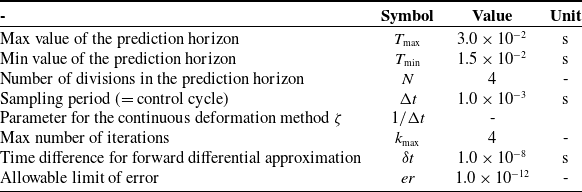
The design parameters used in the NMPC are presented in Table I. The weights of NMPC are then set as follows. The terminal weights are set as
 $\boldsymbol{S}_f=$
diag[0, 6
 $\times$
10
 $^6$
, 20
 $\times$
10
 $^6$
, 15
 $\times$
10
 $^6$
, 10
 $\times$
10
 $^6$
, 0, 11
 $\times$
10
 $^2$
, 85
 $\times$
10, 5
 $\times$
10
 $^2$
, 8
 $\times$
10
 $^2$
, 0, 0, 0, 0]. The state weights in the stage cost are set as
 $\boldsymbol{Q}=$
diag[0, 45
 $\times$
10
 $^5$
, 18
 $\times$
10
 $^6$
, 13
 $\times$
10
 $^6$
, 96
 $\times$
10
 $^5$
, 0, 105
 $\times$
10, 82
 $\times$
10, 45
 $\times$
10, 75
 $\times$
10, 0, 0, 0, 0]. The input weights in the stage cost are set as
 $\boldsymbol{R}=$
diag[6
 $\times$
10
 $^{-2}$
, 15
 $\times$
10
 $^{-3}$
, 8
 $\times$
10
 $^{-2}$
, 2
 $\times$
10
 $^{-2}$
]. These NMPC parameter settings need to be determined through a trial-and-error process; however, tuning some of the parameters may potentially benefit from the methods described in reference [Reference Lu42].
4.1.3. Simulation setup
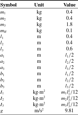
The physical parameters of the robot used in the numerical simulations are listed in Table II. The simulation comprises of MATLAB 2024a, Ryzen 9 9950X processor, 64 GB RAM, and Windows 11. The walking pattern established using these parameters is considered steady walking from the 15th step onward. The robot’s walking speed and SR value, an index for evaluating energy efficiency, were calculated using walking data from the 15th to the 25th steps. The SR is defined as:
 \begin{equation} \mathrm{SR}\,:\!=\, \frac {p}{Mgv_{a}}, \end{equation}
where
 $p$
[J/s] is the average input power,
 $M$
[kg] is the total weight of the robot, and
 $v_a$
[m/s] is the average walking speed of the robot. For the five-link bipedal robot used in this study,
 $p$
can be calculated using the following equation:
 \begin{align*} p\,:\!=\,\frac {1}{T_{t}} \int _0^{T_{t}} (|u_1(\dot {\theta }_2-\dot {\theta }_1)|+|u_2(\dot {\theta }_3-\dot {\theta }_5)|+|u_3(\dot {\theta }_4-\dot {\theta }_3)| +|u_4(\dot {\theta }_5-\dot {\theta }_2)|) \mathrm{dt}, \end{align*}
where
 $T_{t}$
[s] is the total walking time.
Control parameters for NMPC.

Physical parameters for the five-link biped robot.

4.2. Walking under ideal environments
4.2.1. OZC-based walking
Variations in the torso angle during OZC-based walking with respect to time.

Variations in
 $u_4$
during OZC-based walking with respect to time.

Variations in
 $\phi$
during OZC-based walking with respect to time.

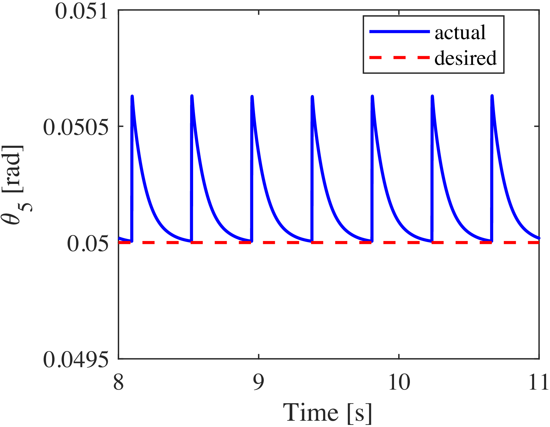
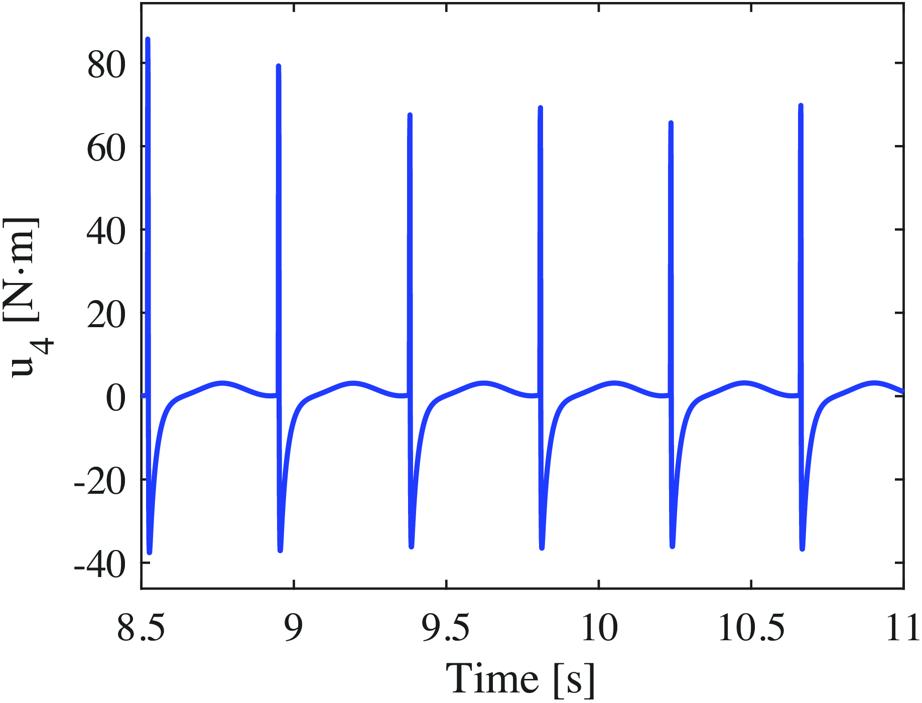
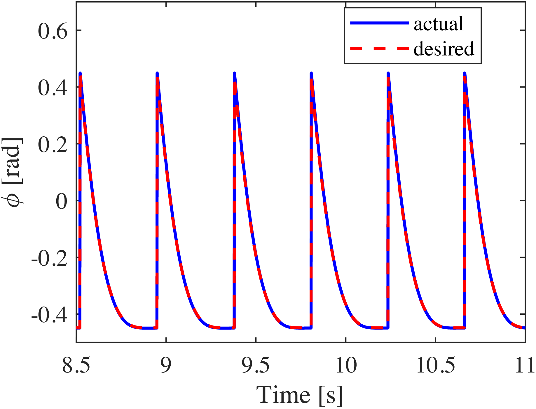
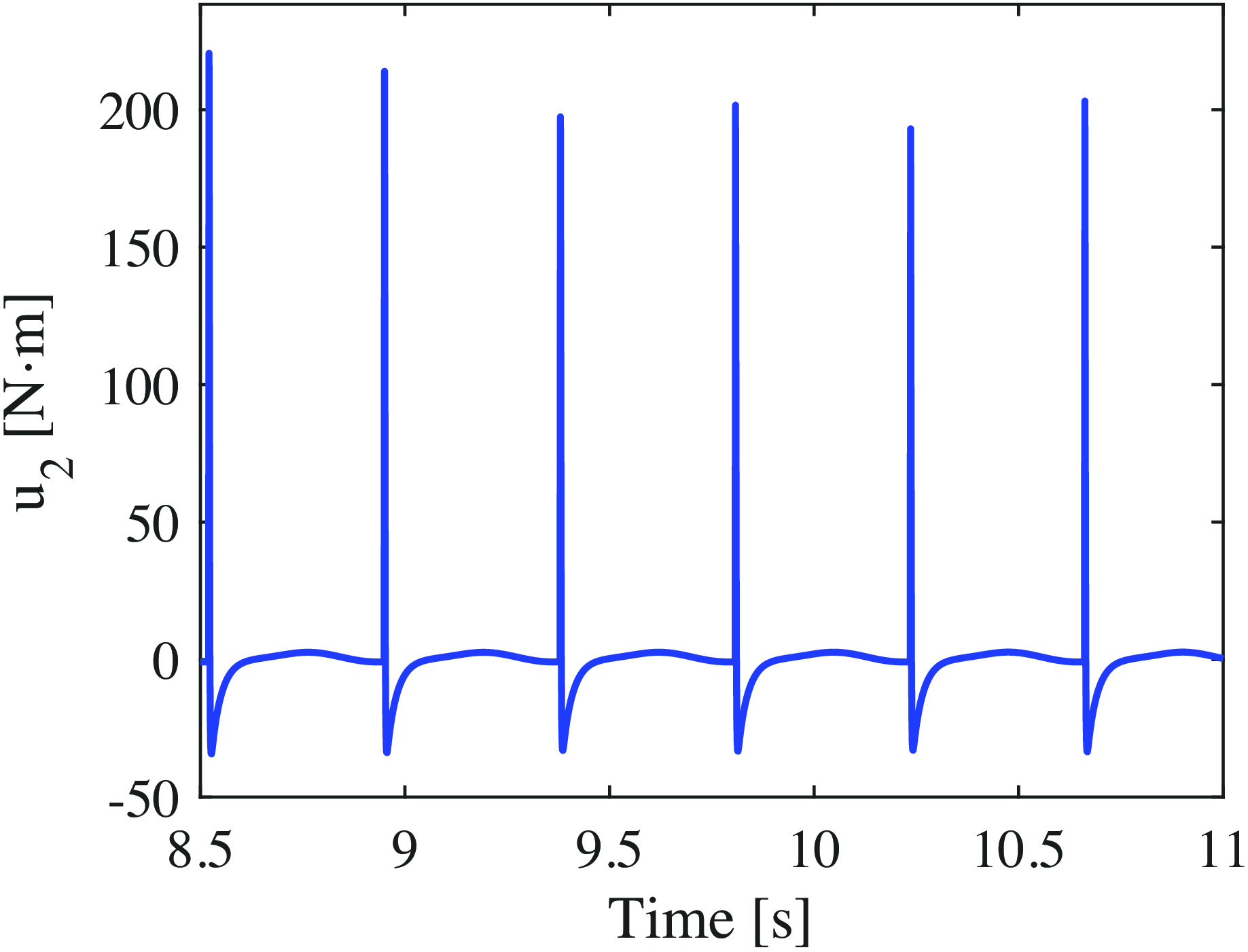
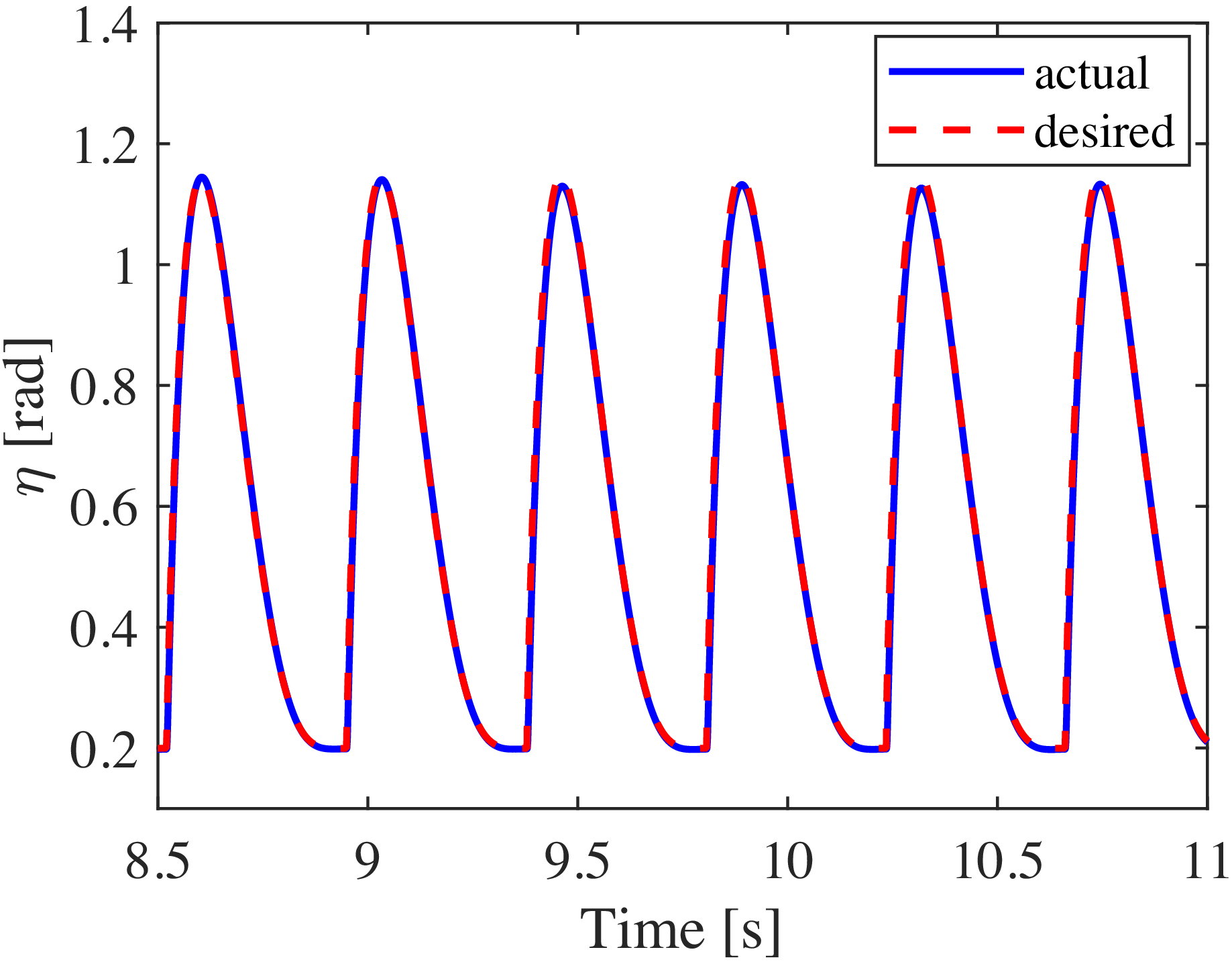
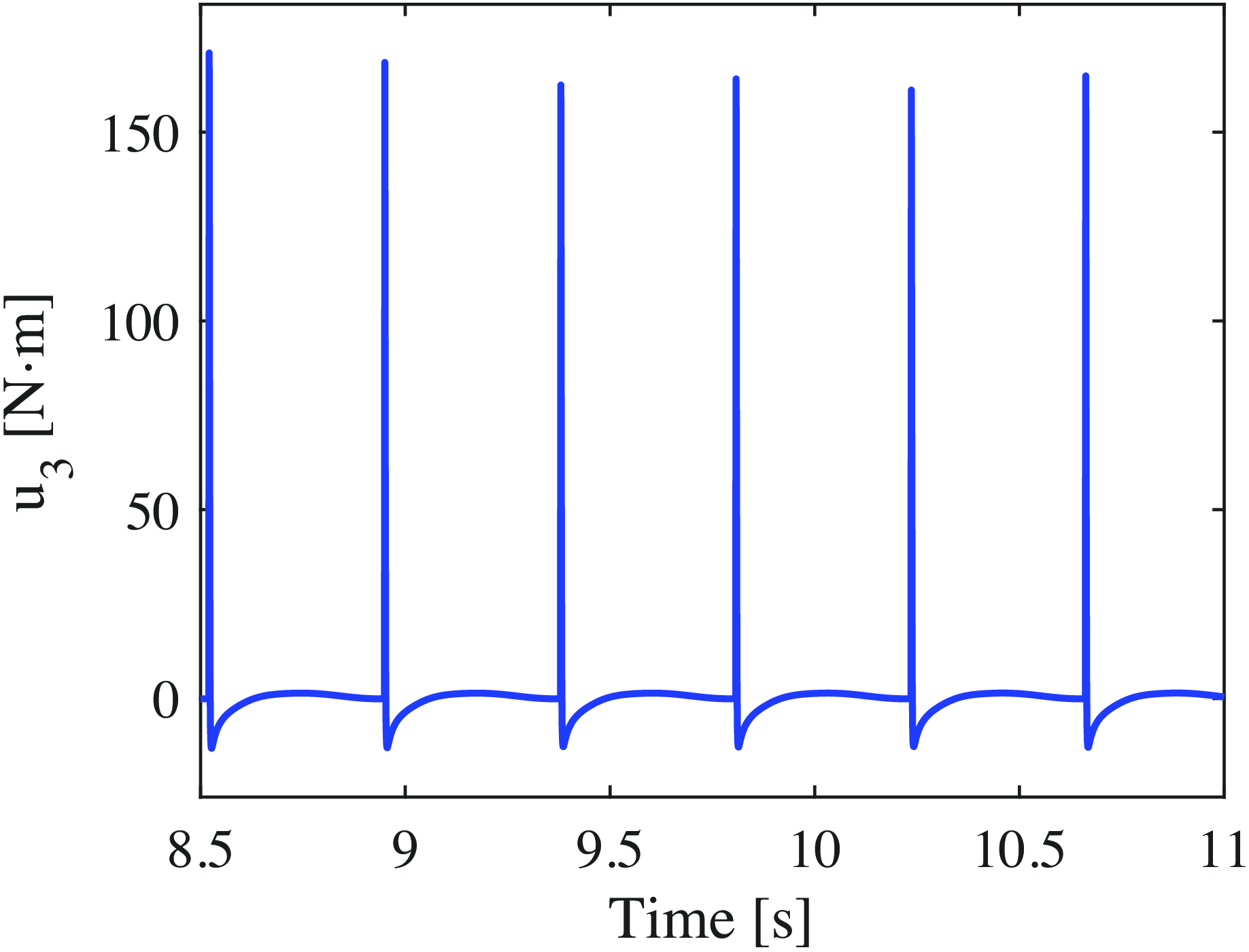
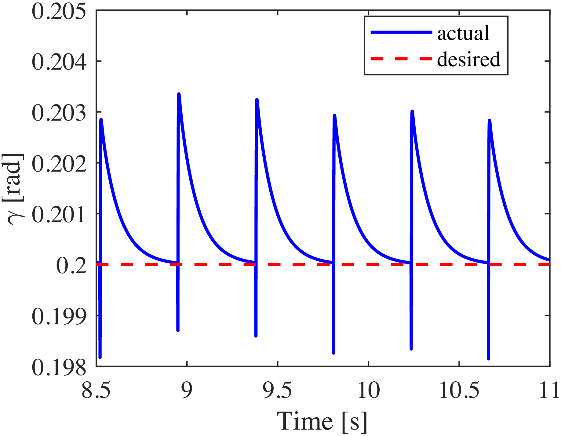
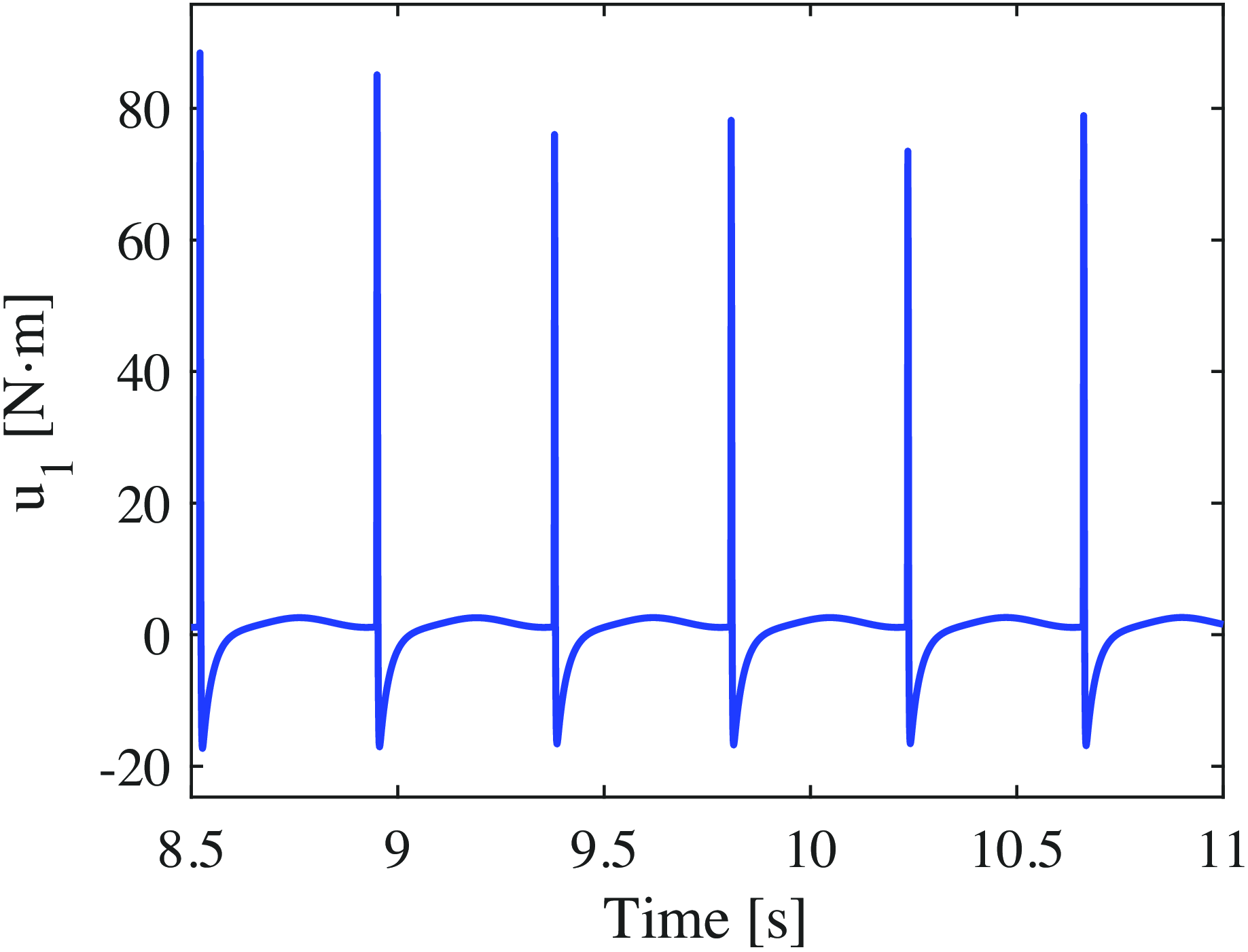
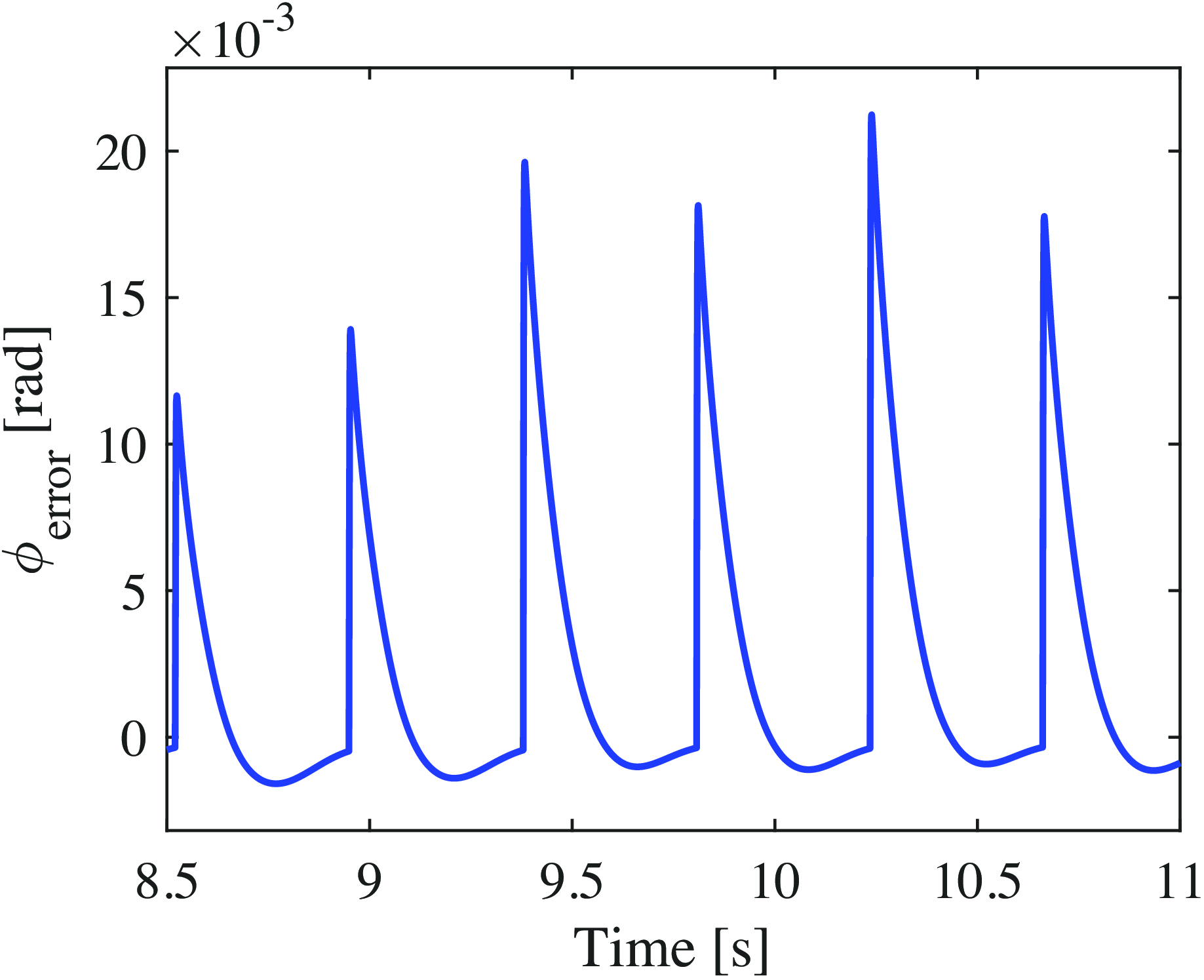
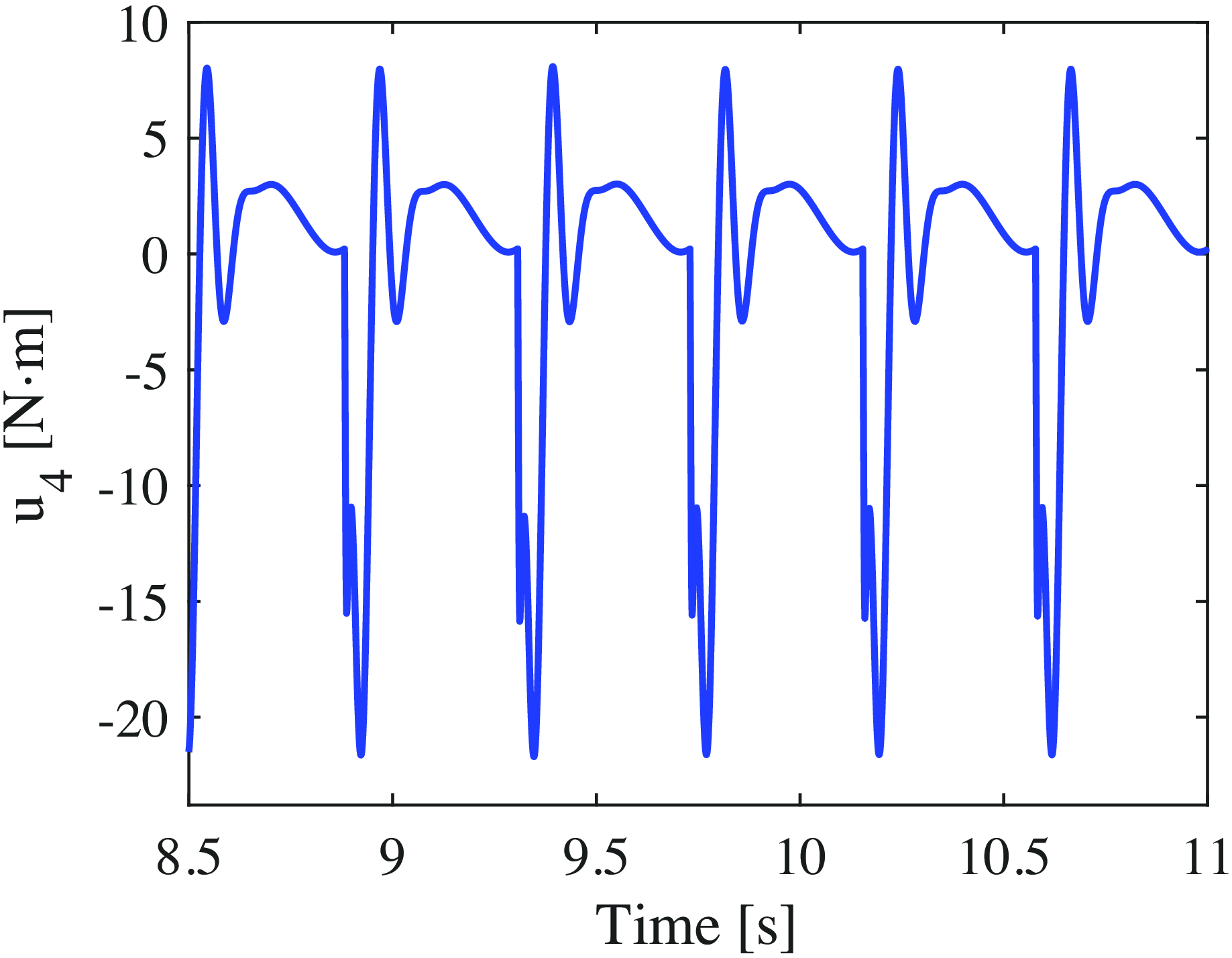
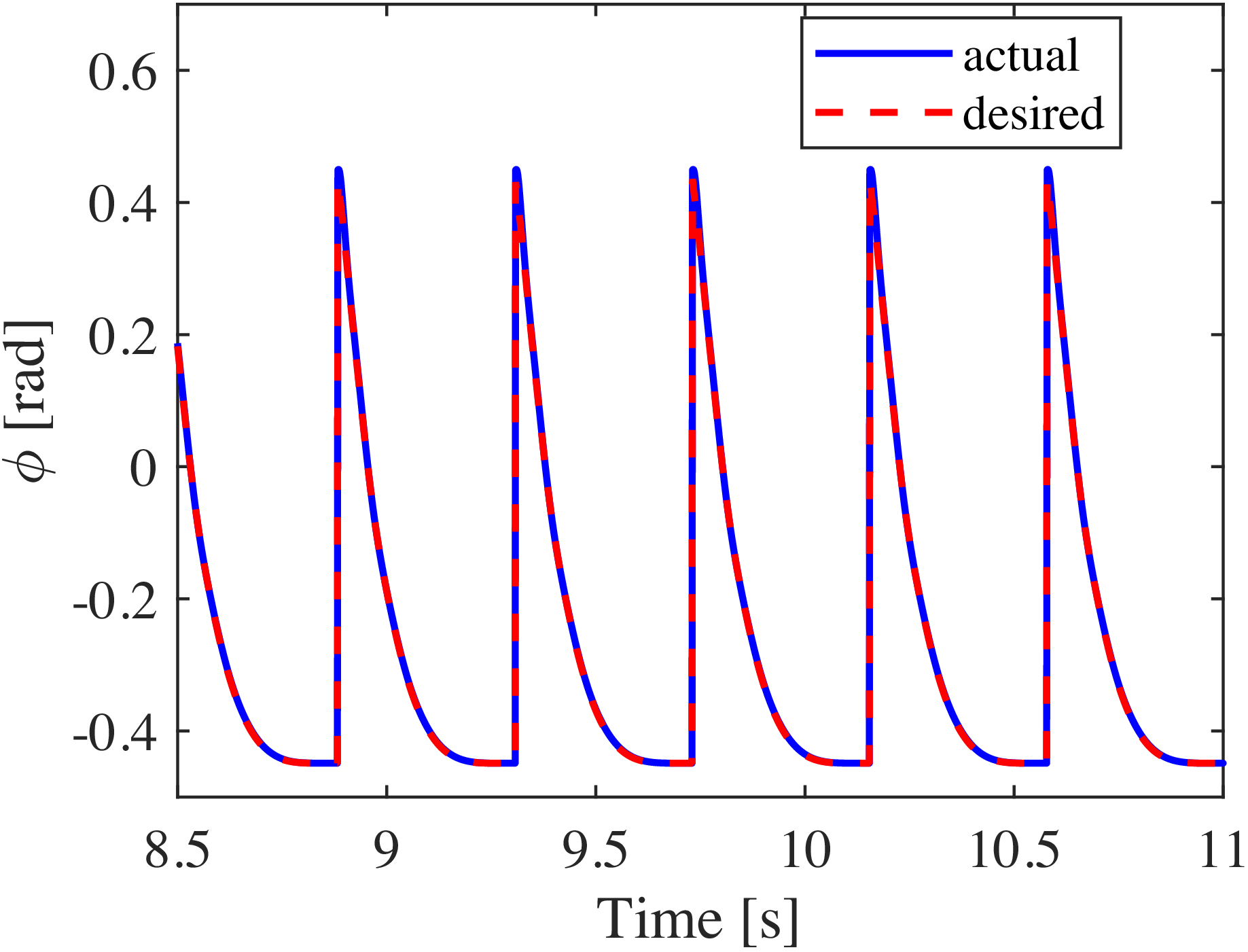
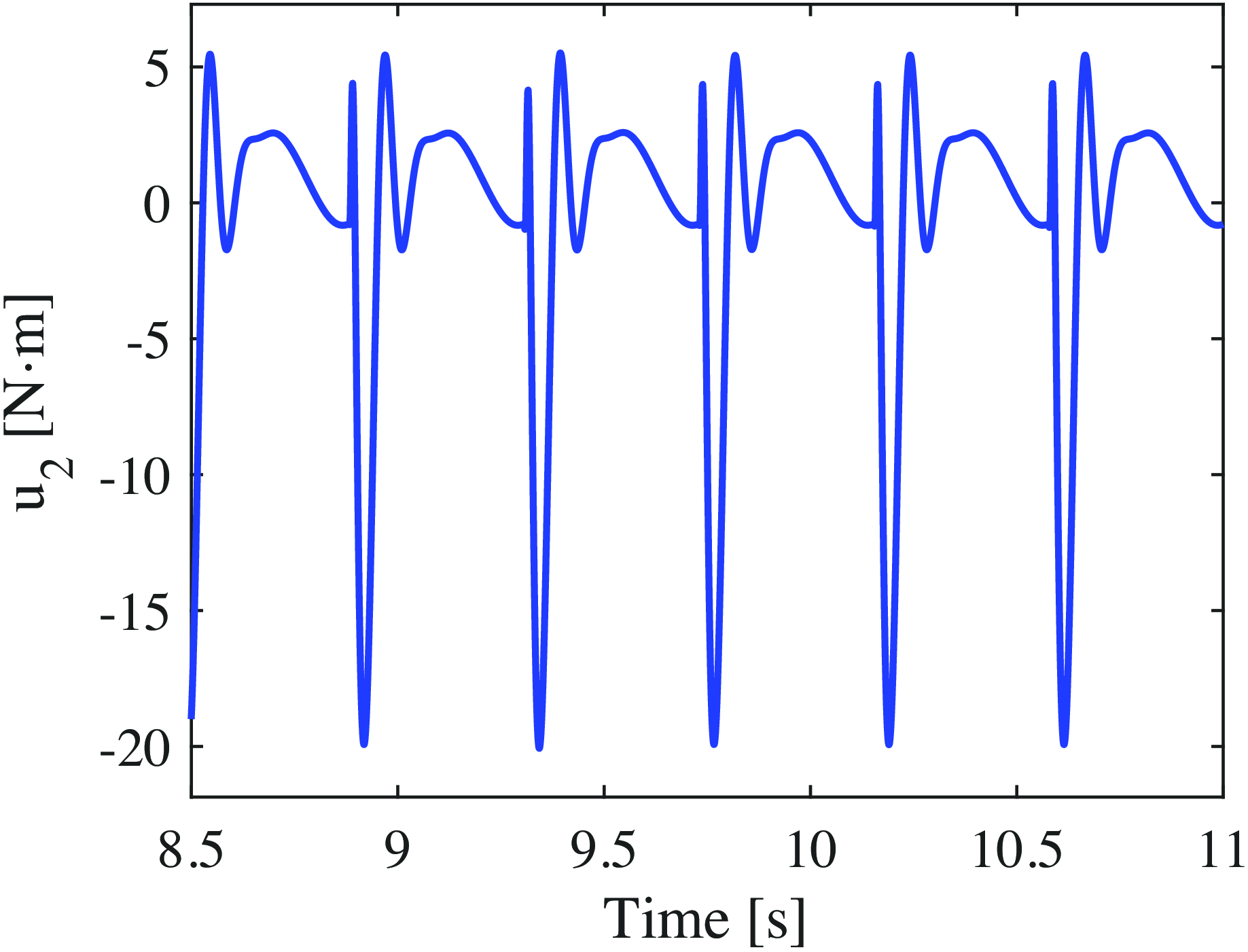
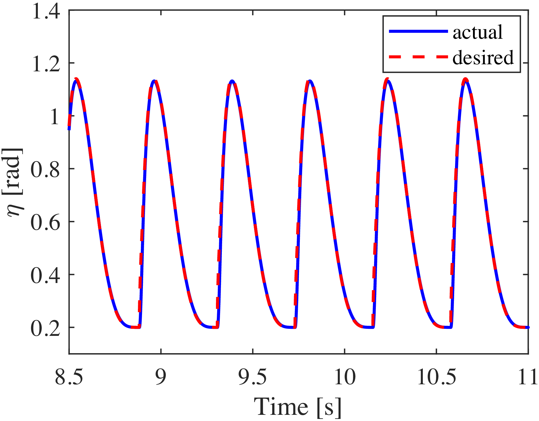
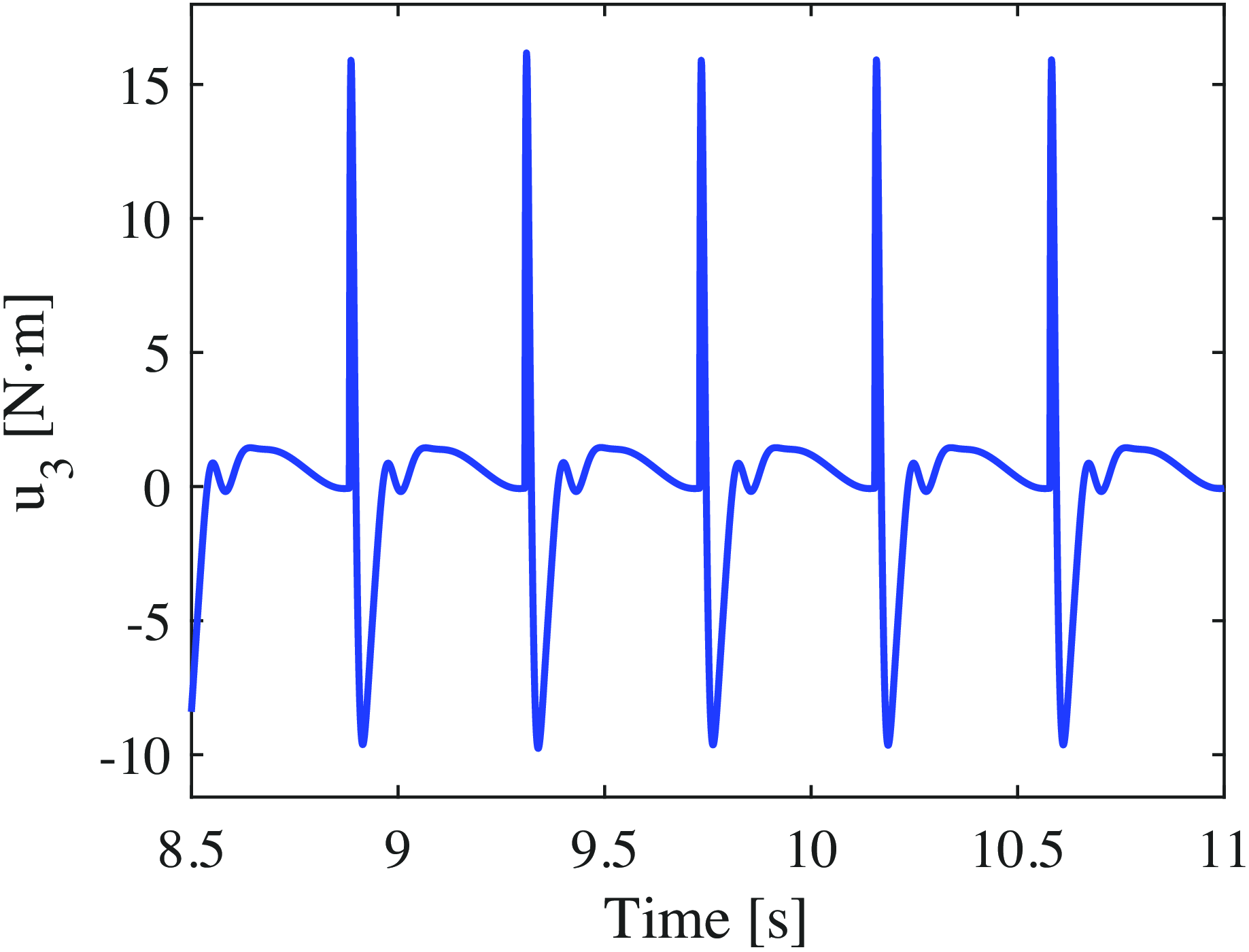
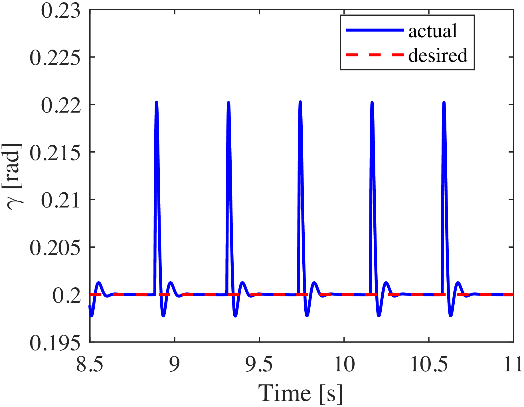
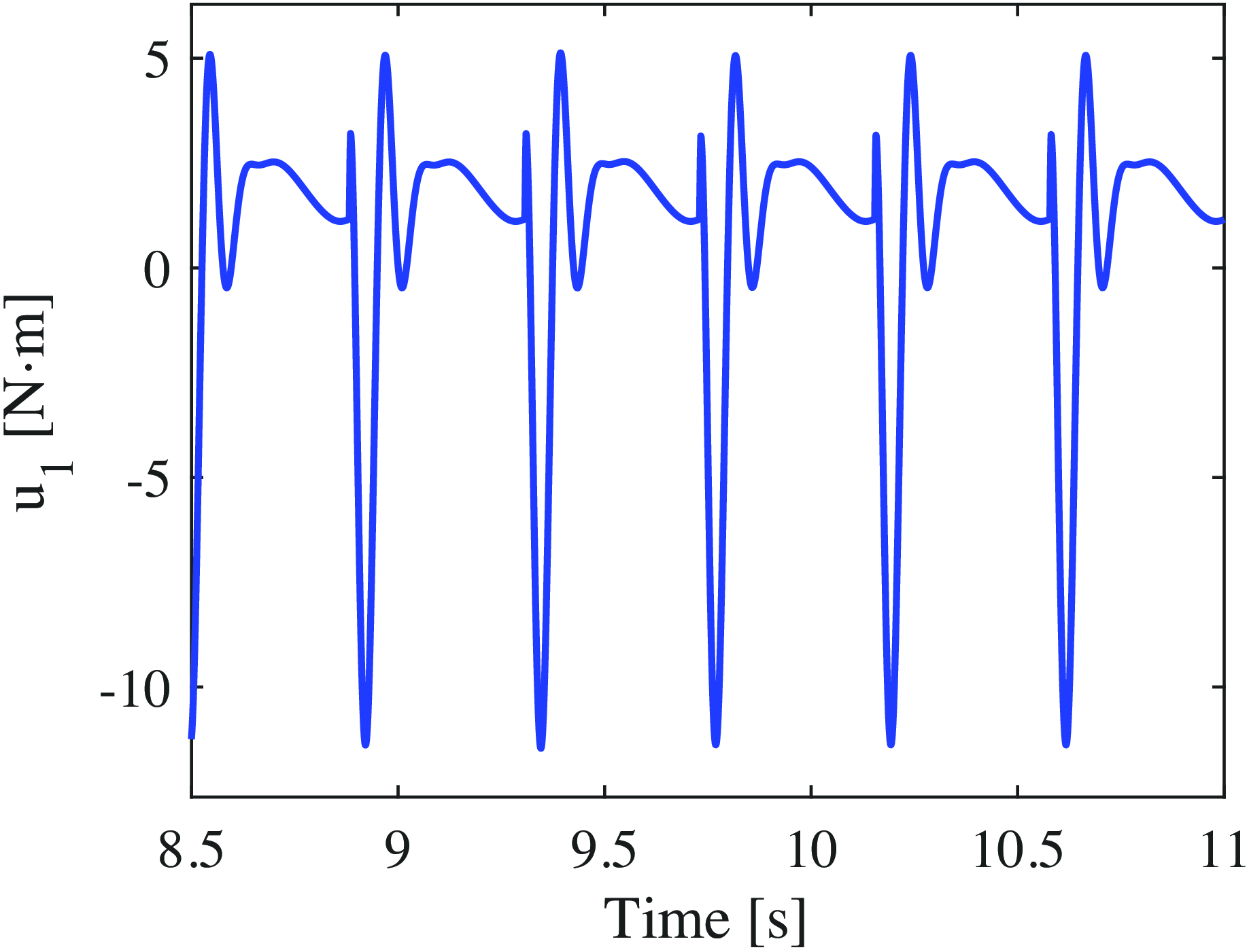
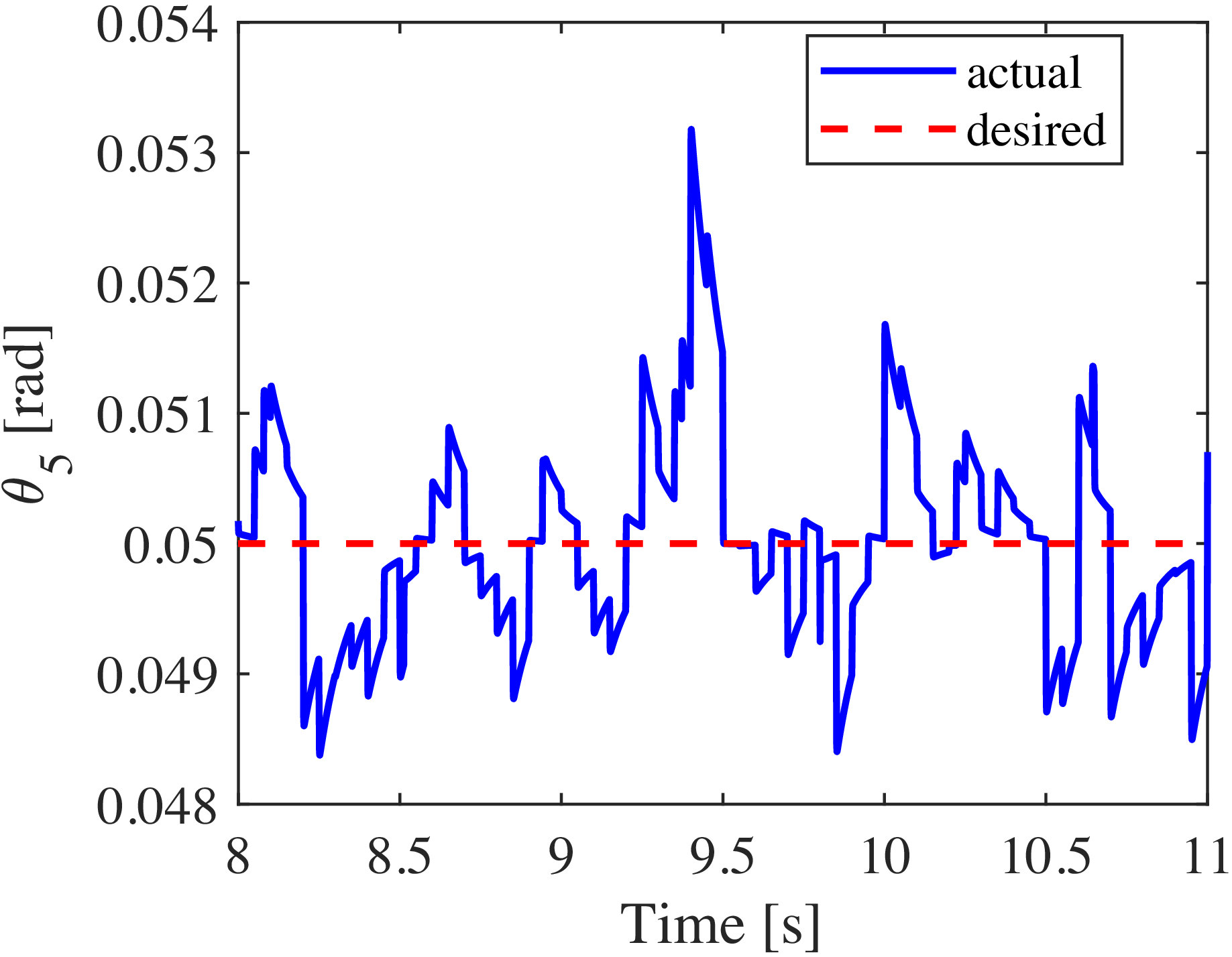
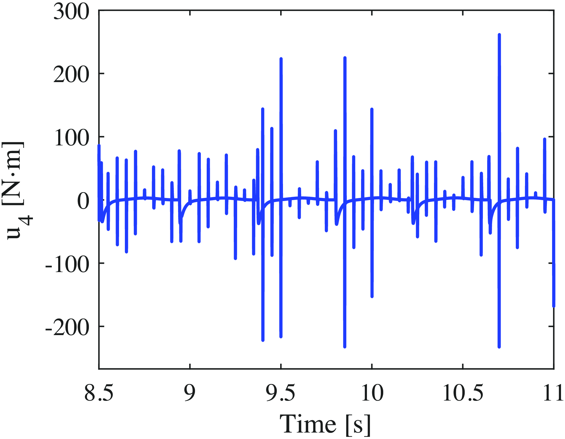
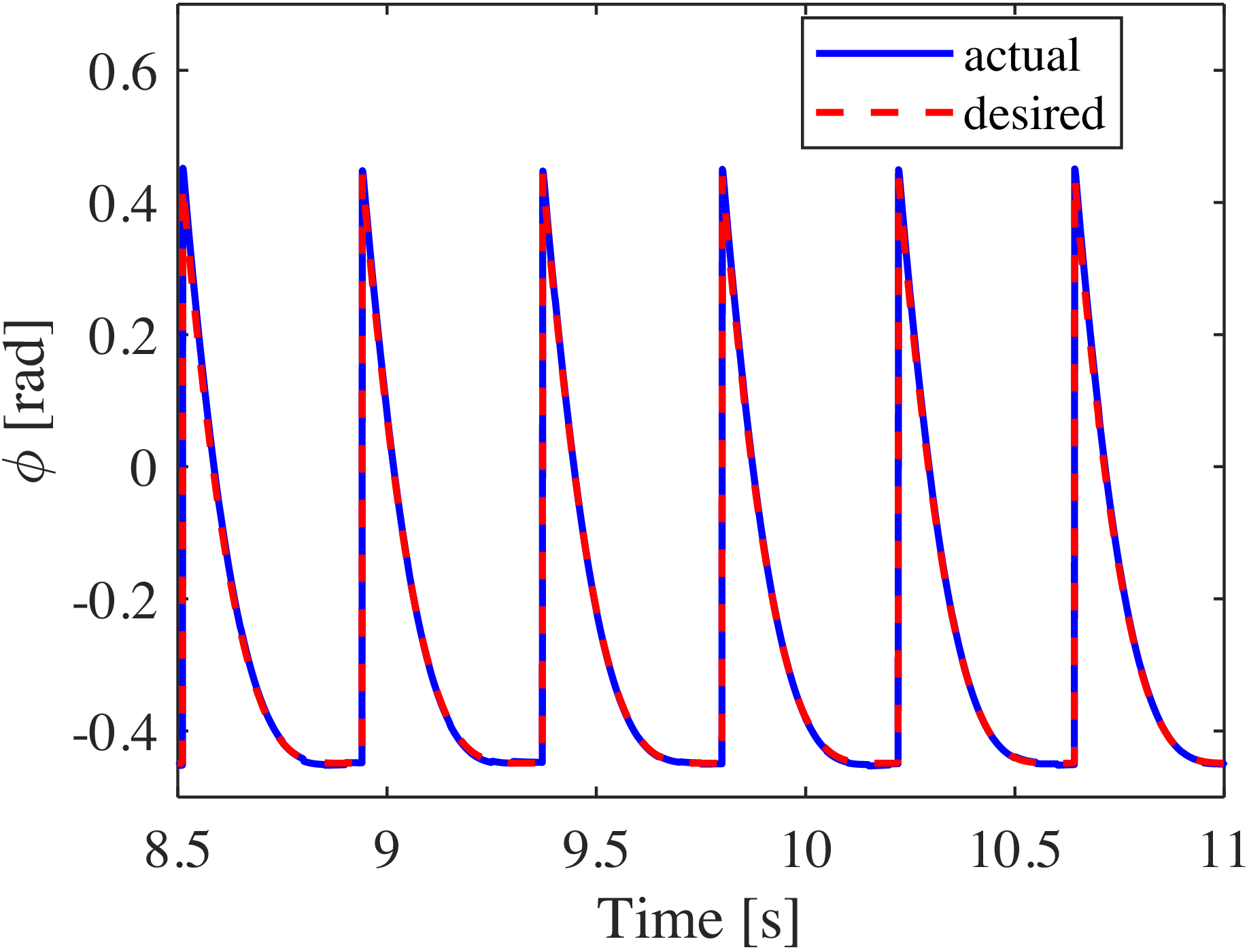
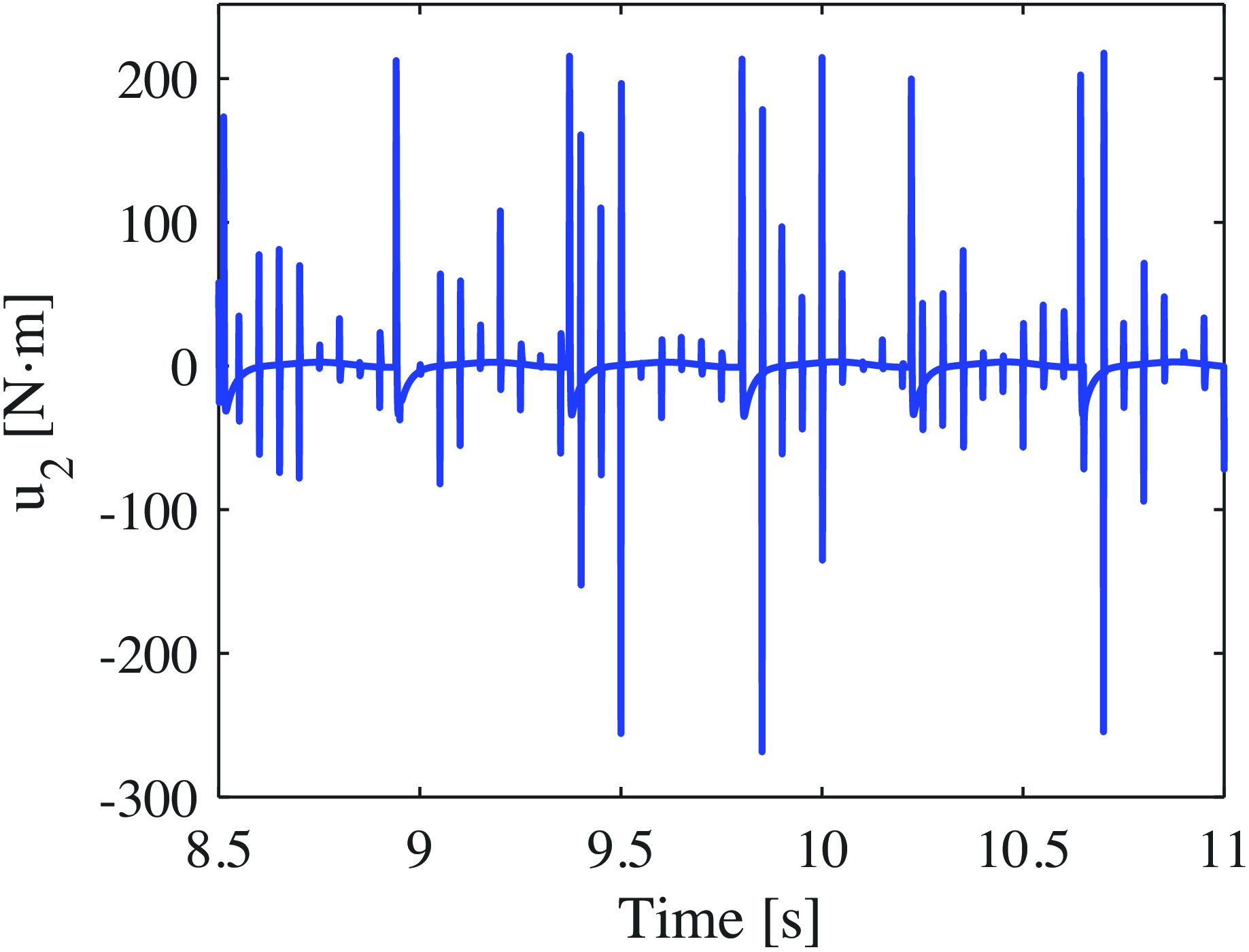
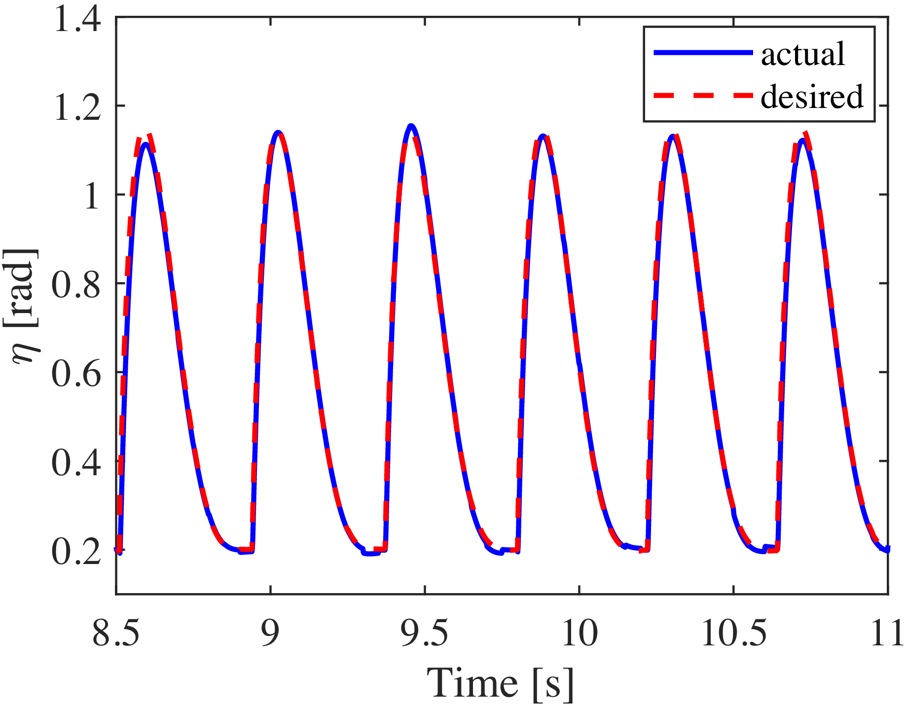
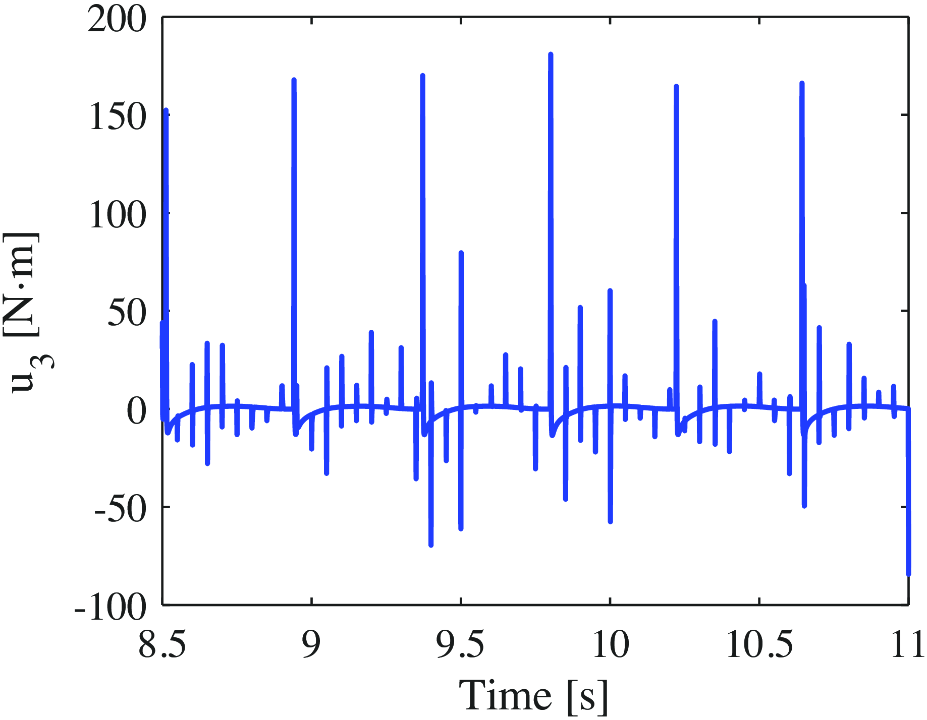
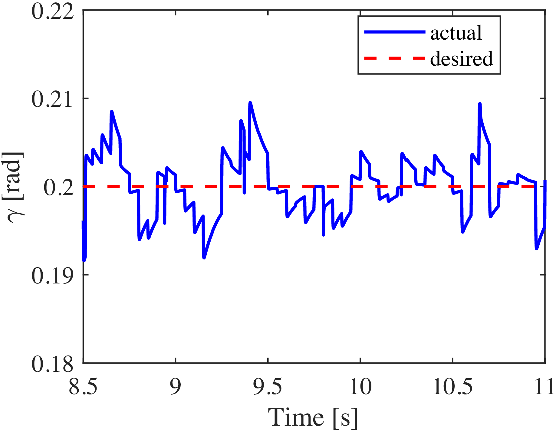
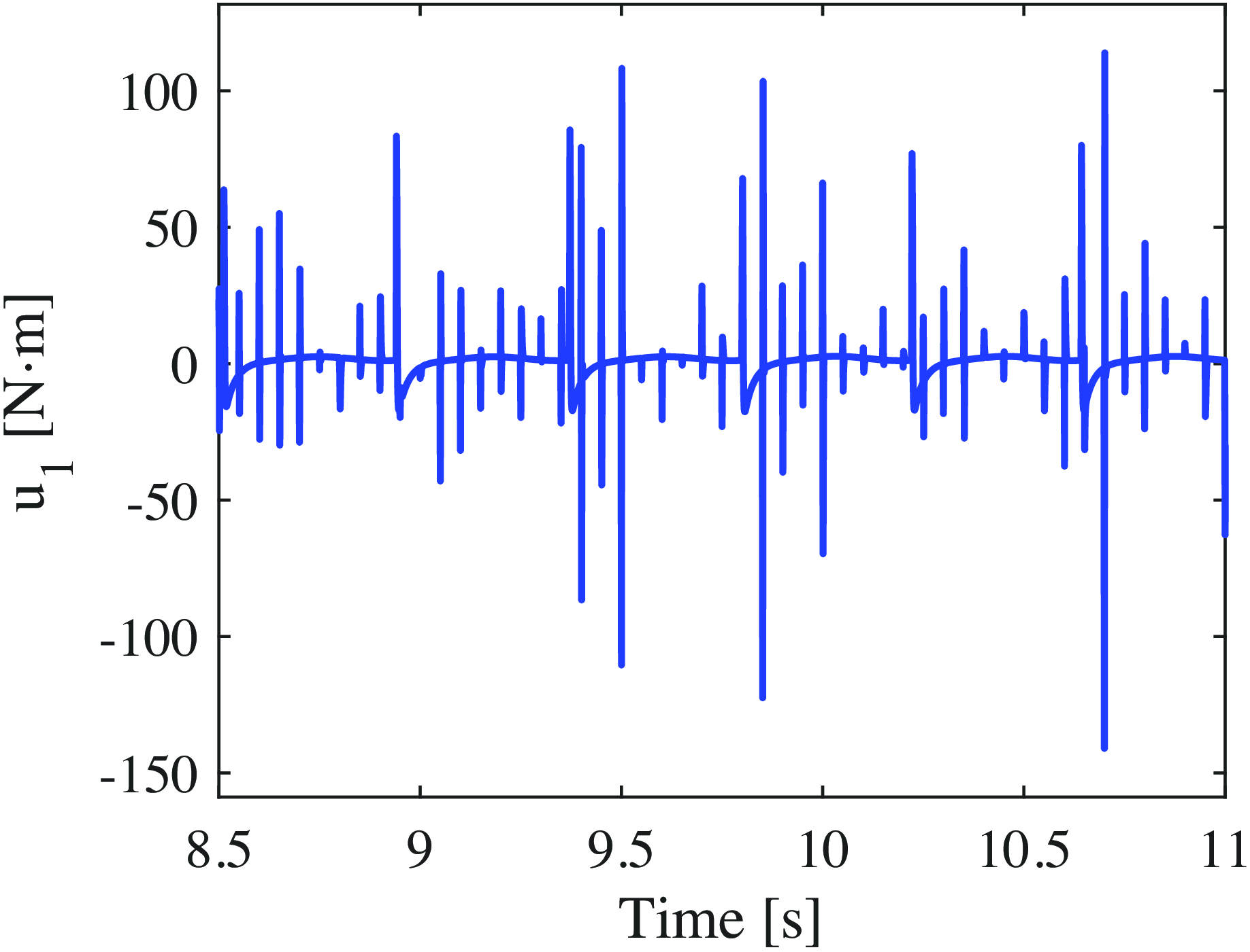
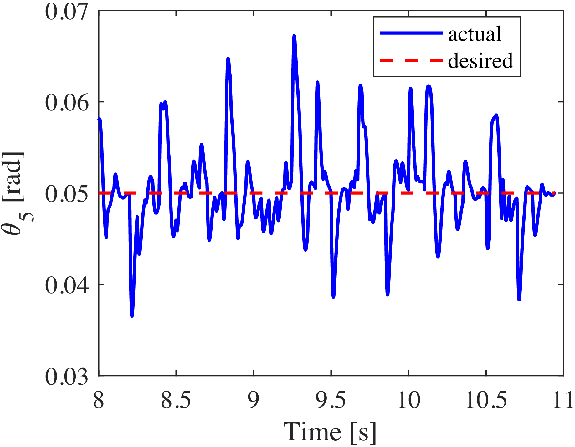
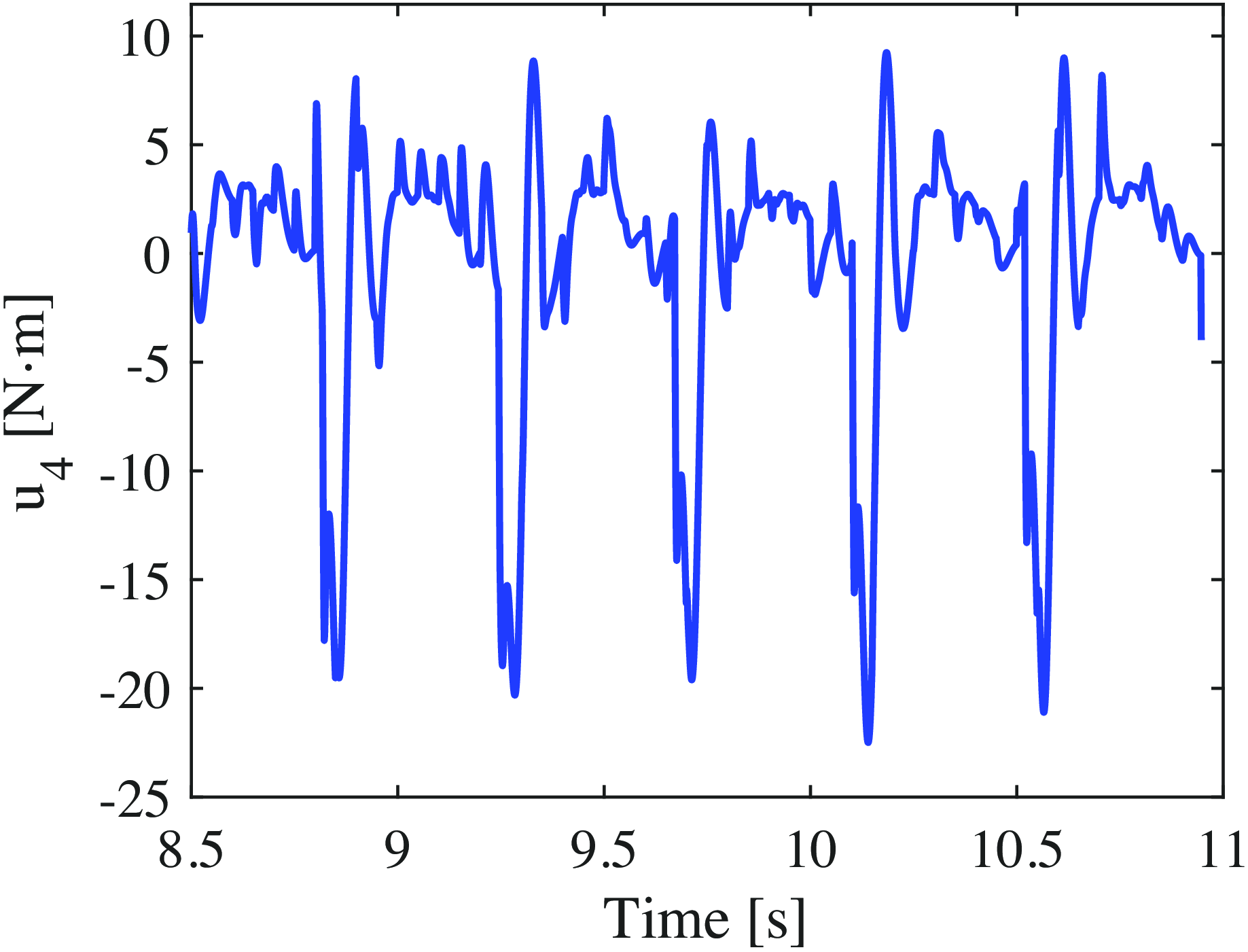
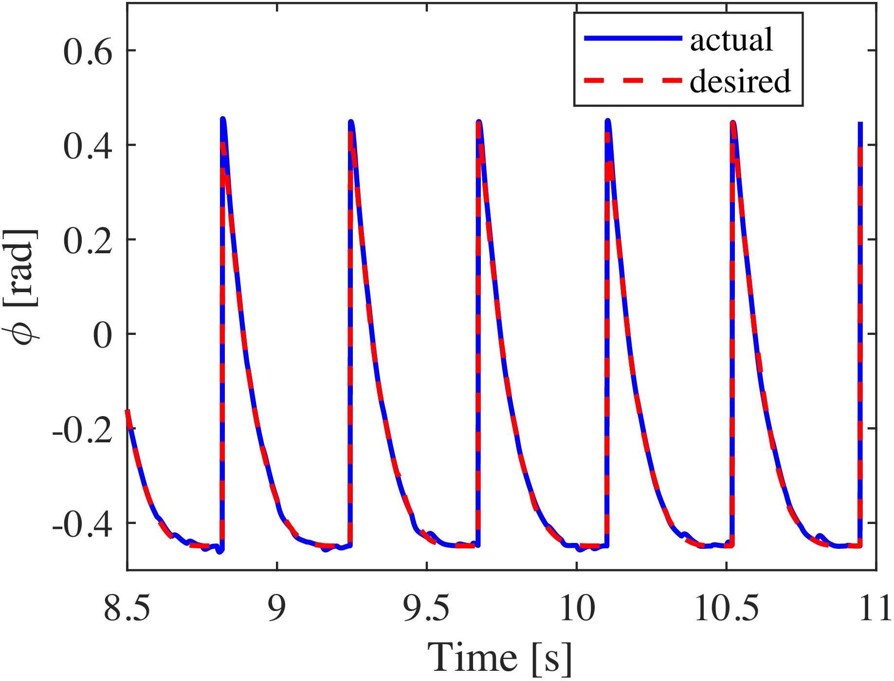
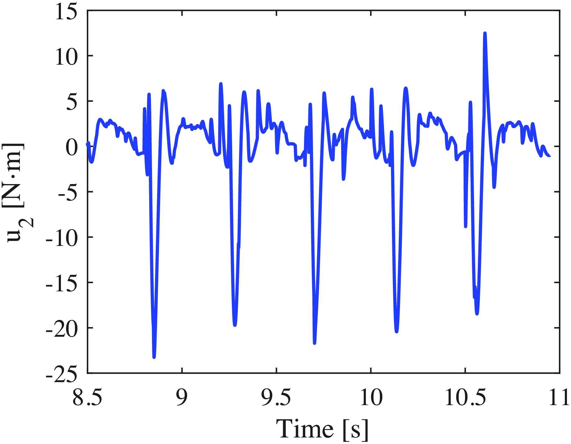
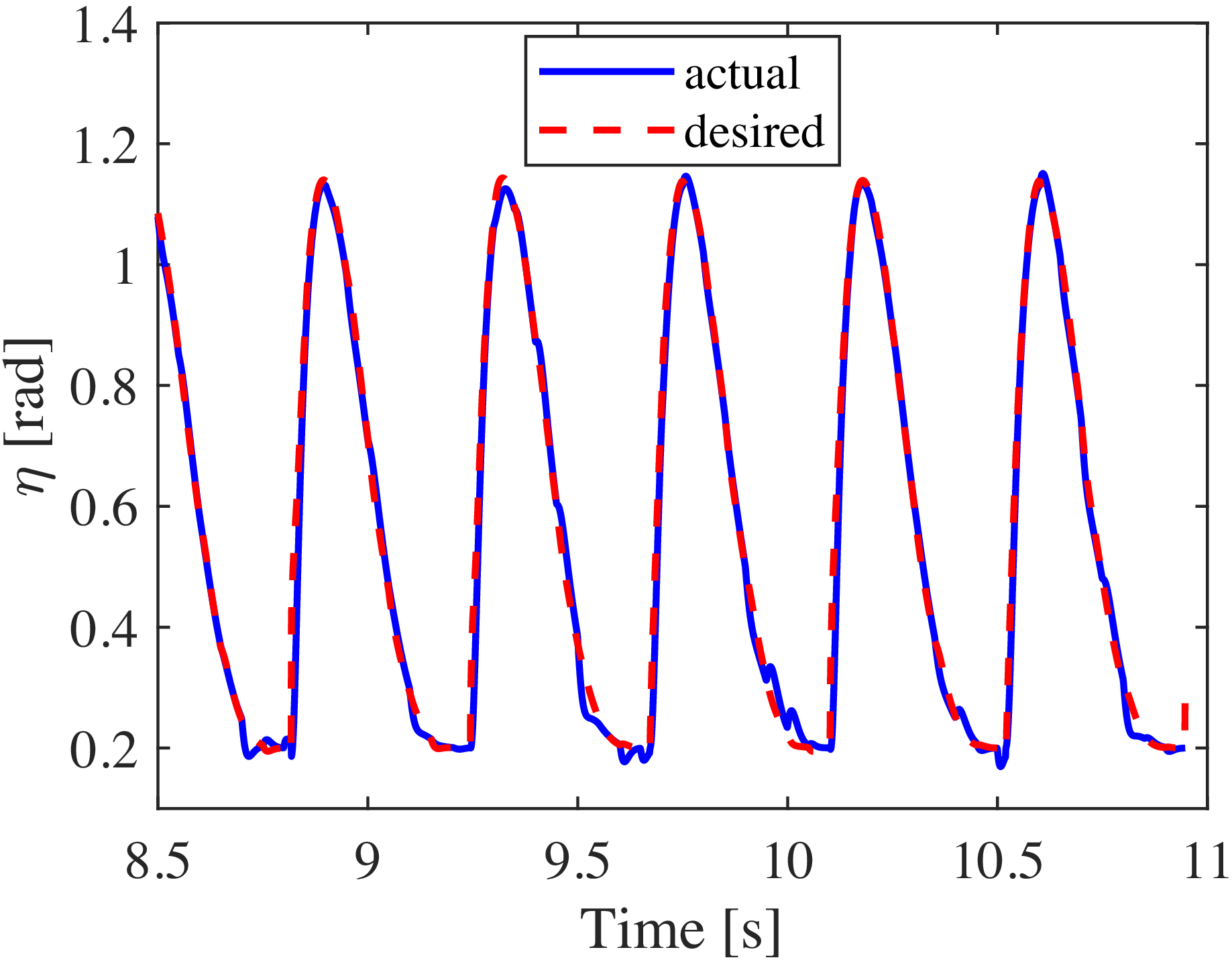
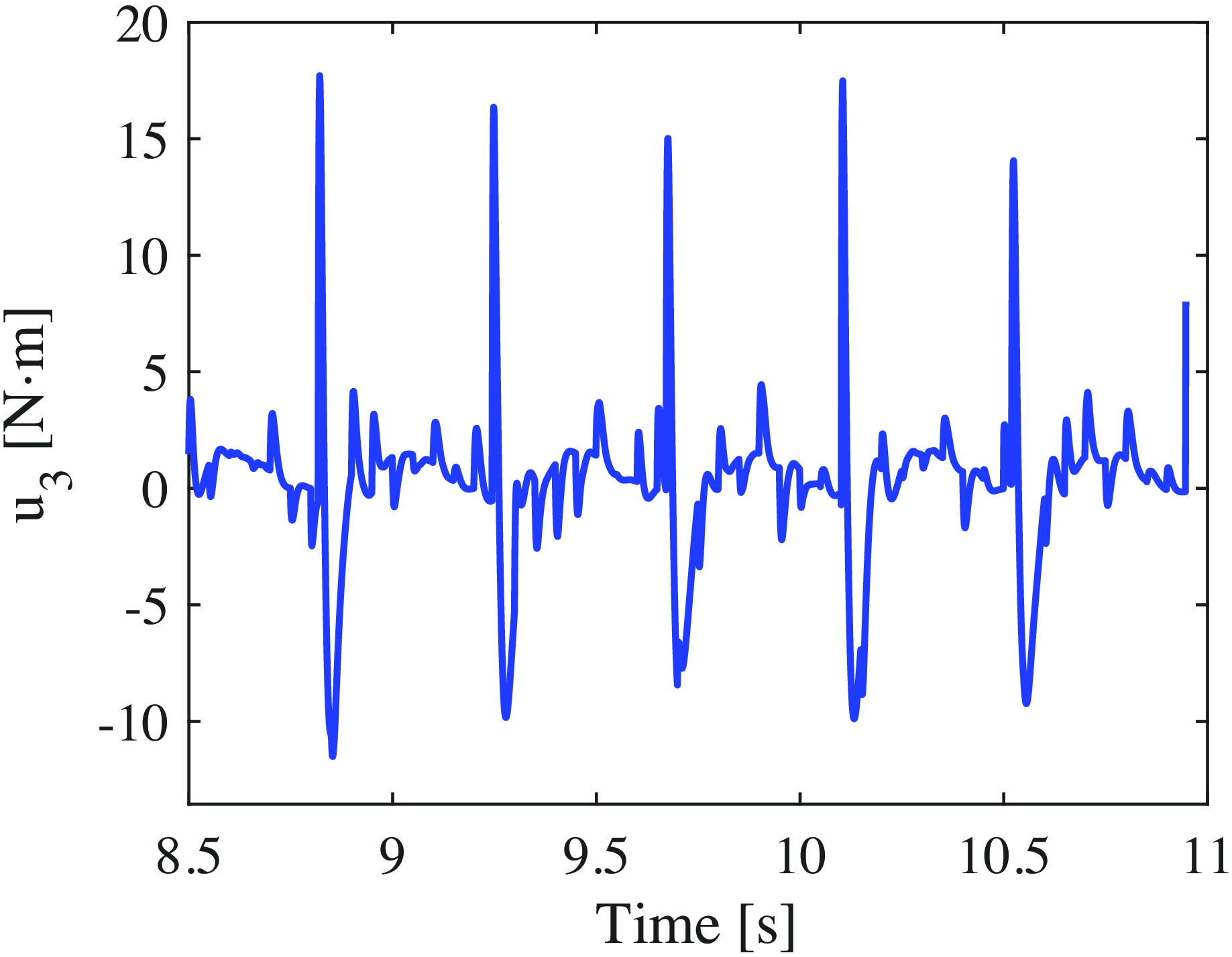
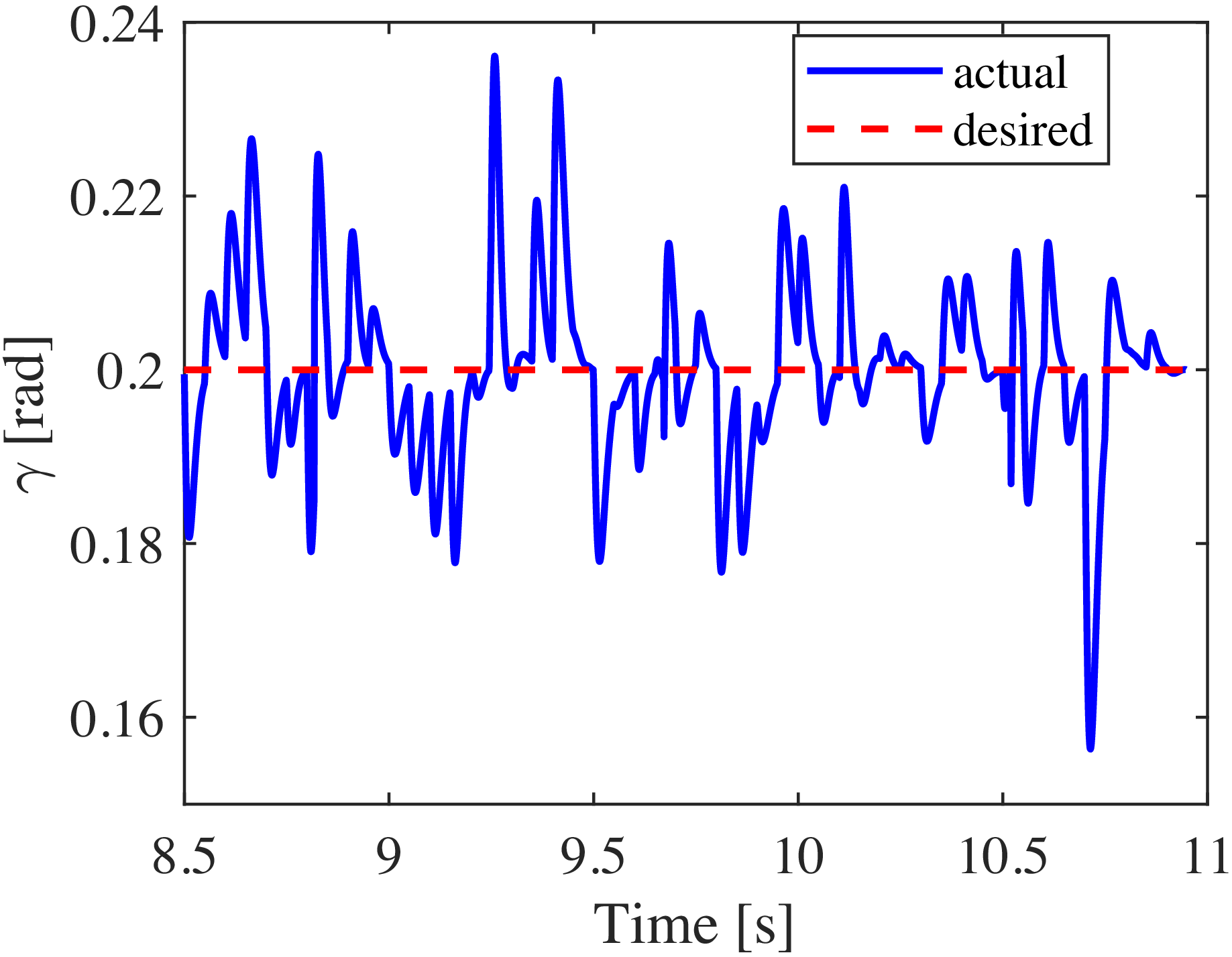
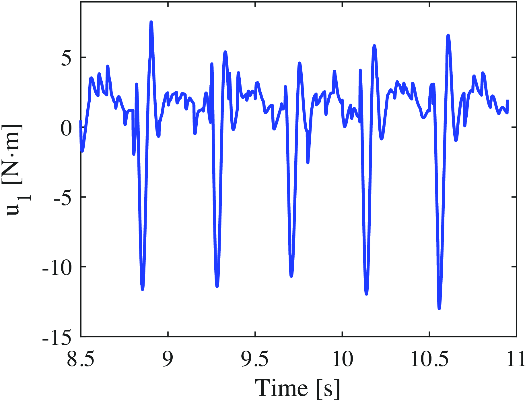
First, the walking pattern using the conventional OZC method is presented. Figures 9–16 show the time-dependent changes in
 $\theta _5$
,
 $u_4$
,
 $\phi$
,
 $u_2$
,
 $\eta$
,
 $u_3$
,
 $\gamma$
, and
 $u_1$
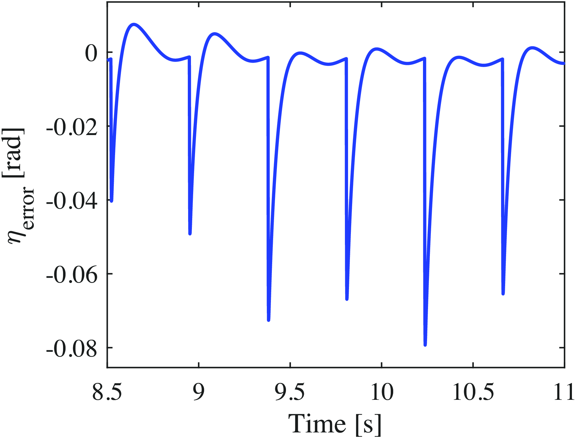
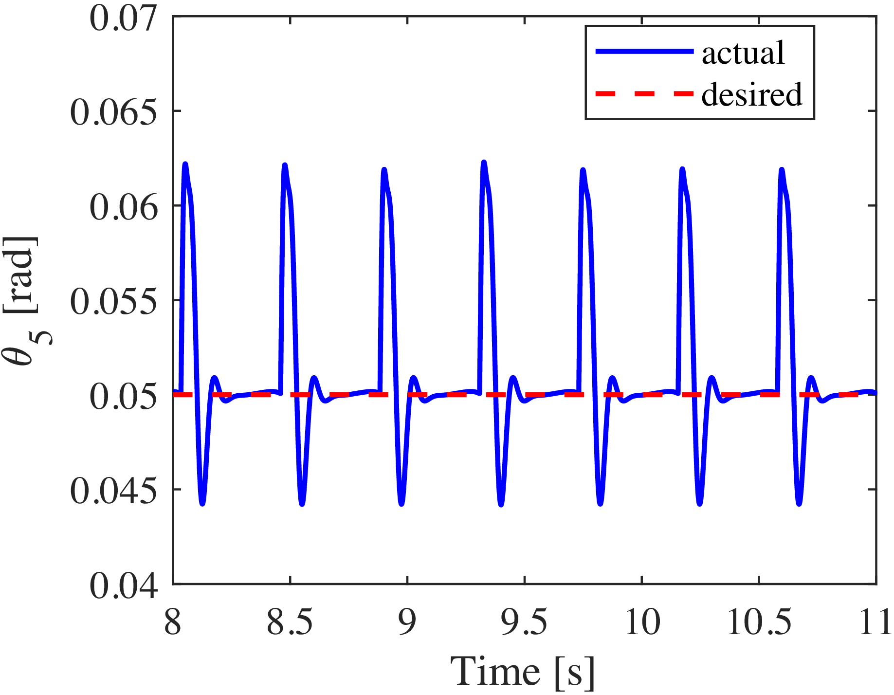
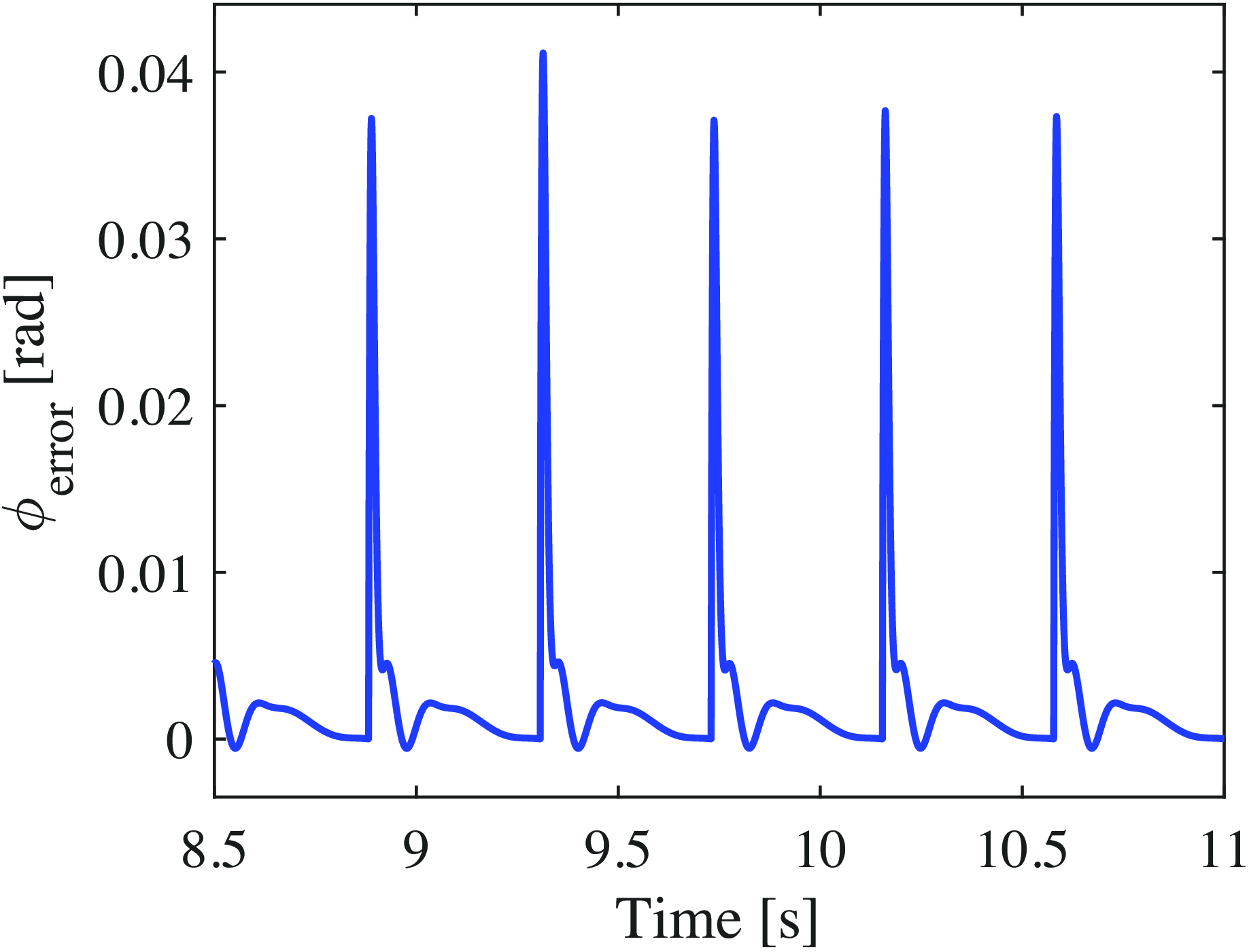
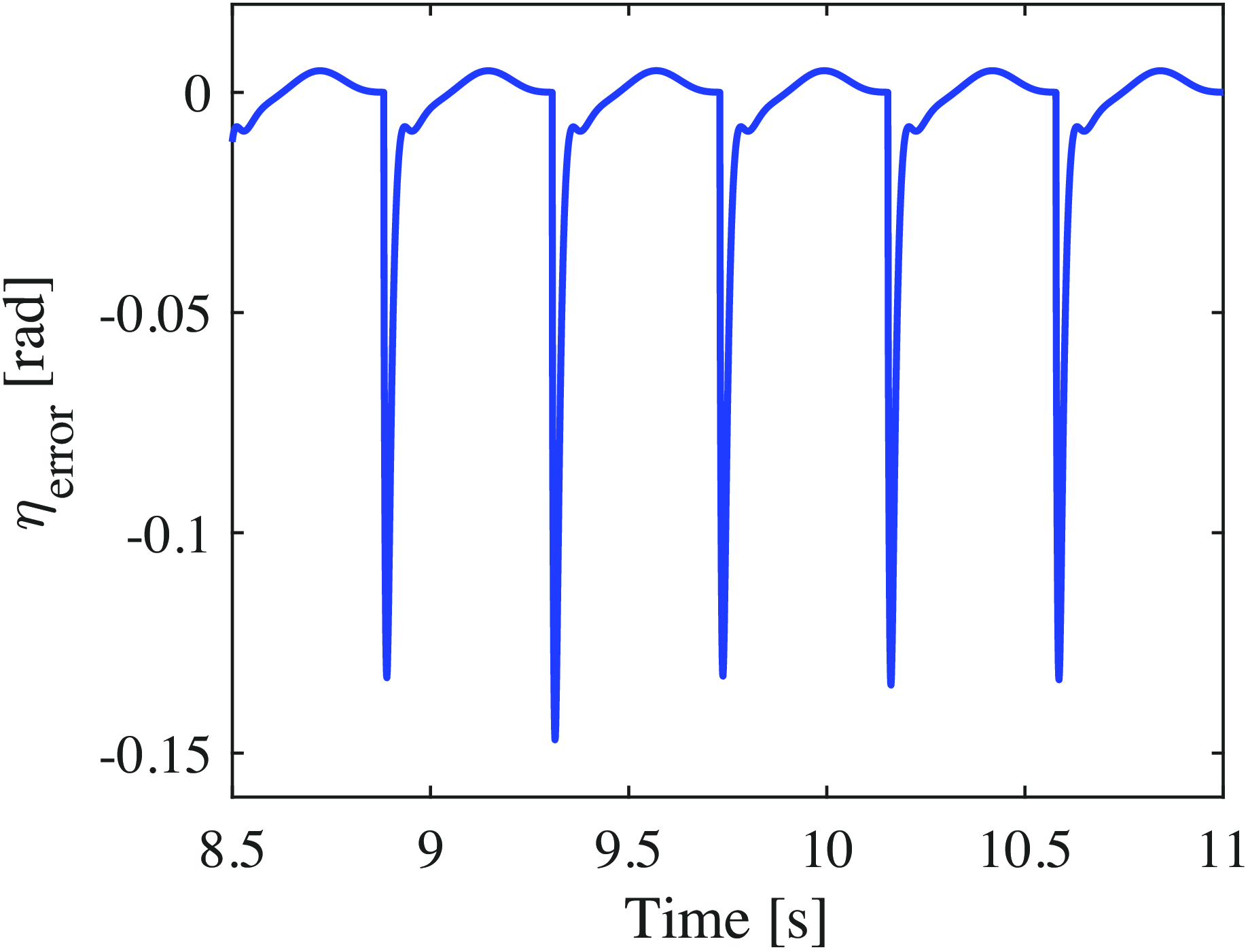
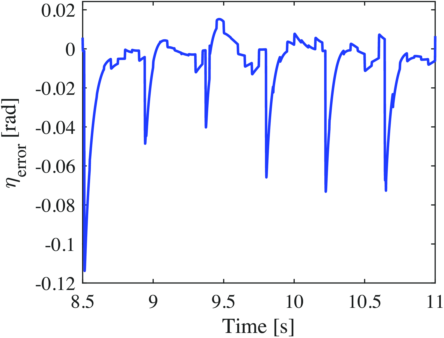
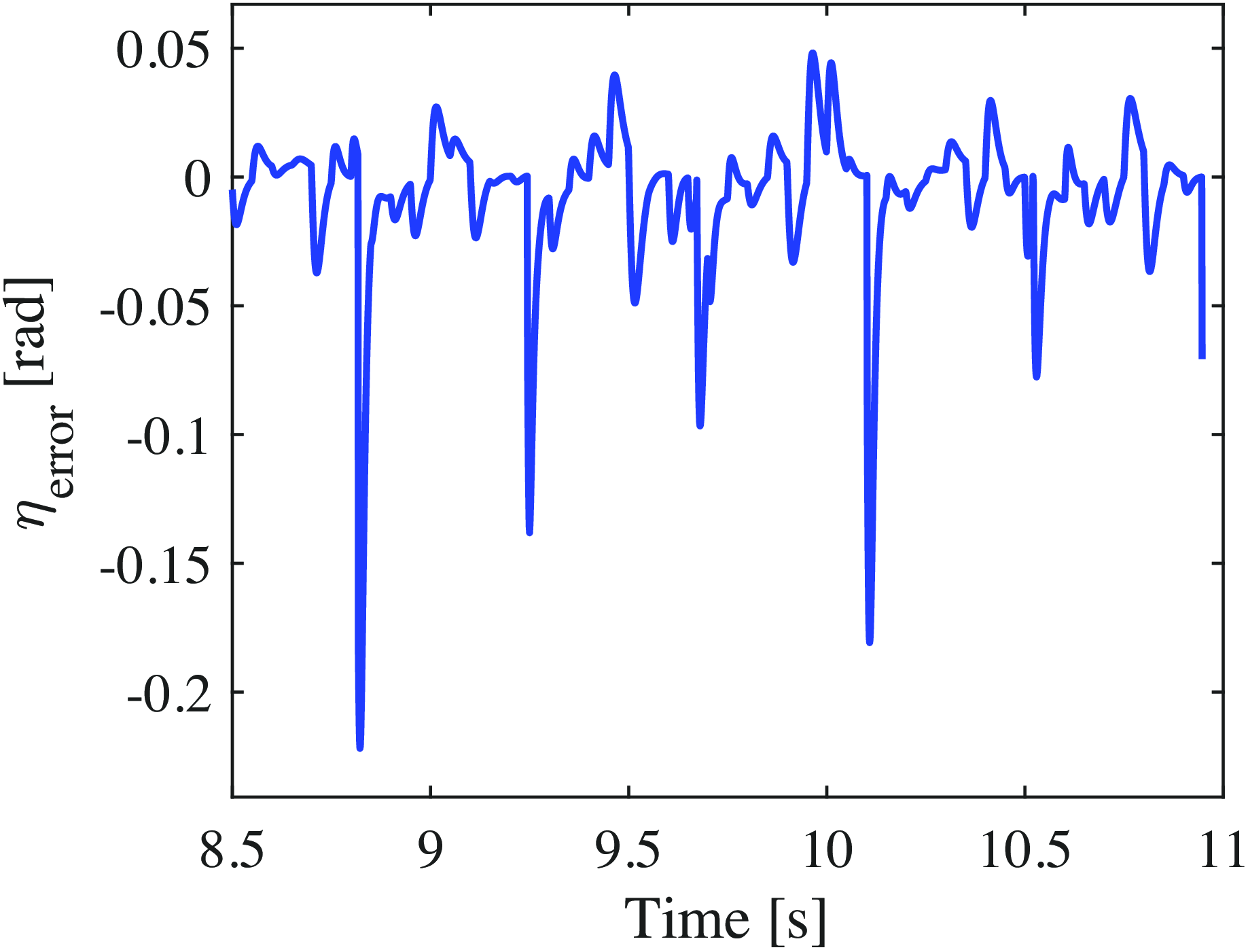
obtained during steady-state walking using the OZC-based approach in ideal environments, respectively. Evidently, the OZC method ensures that the robot strictly adheres to the desired trajectory. However, spike-like torques are observed at each input, occurring immediately after the support leg is switched. Figures 17 and 18 show the errors between the desired values,
 $\phi _d$
,
 $\eta _d$
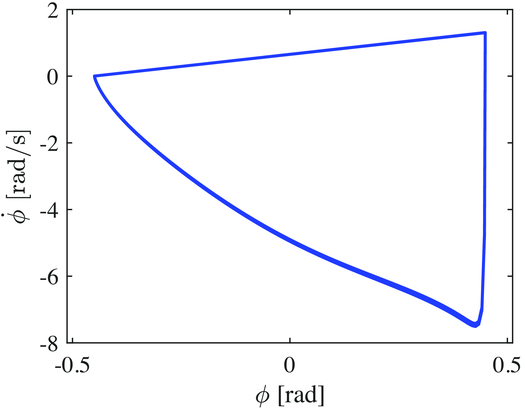
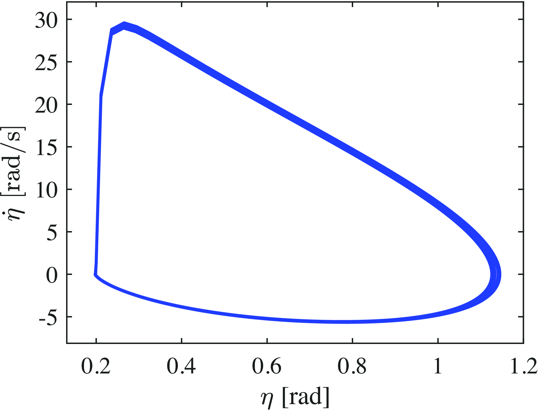
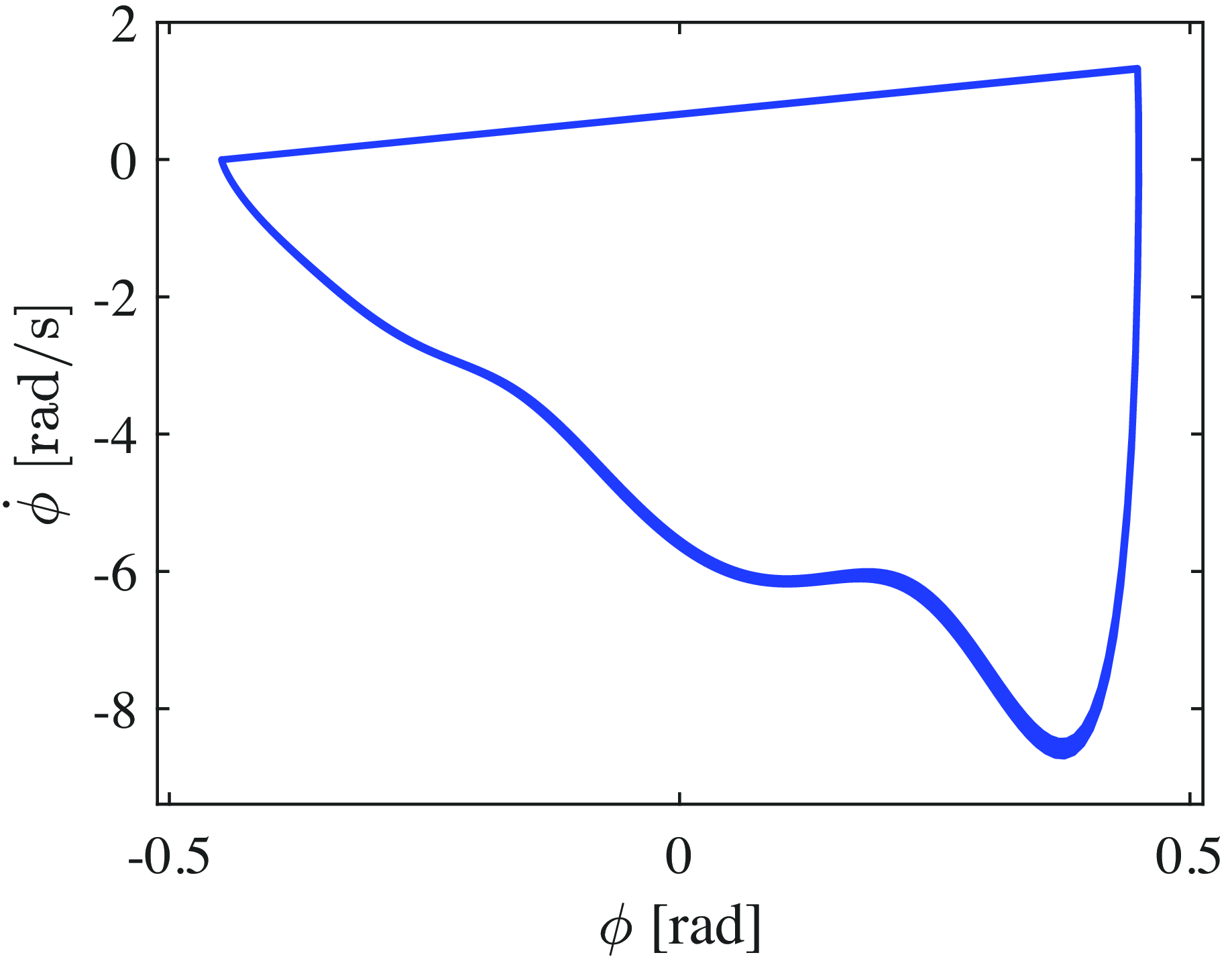
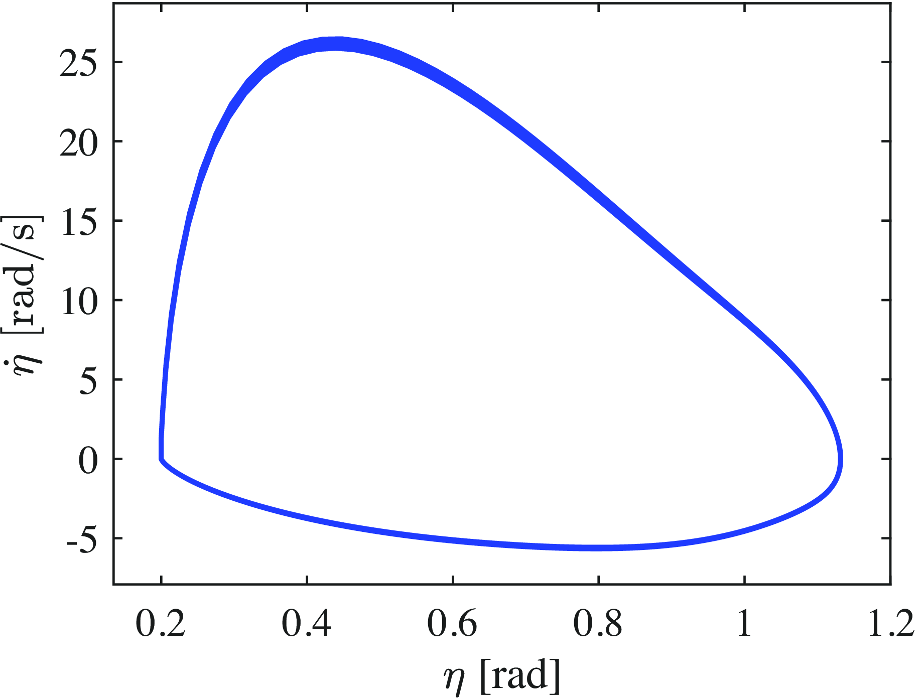
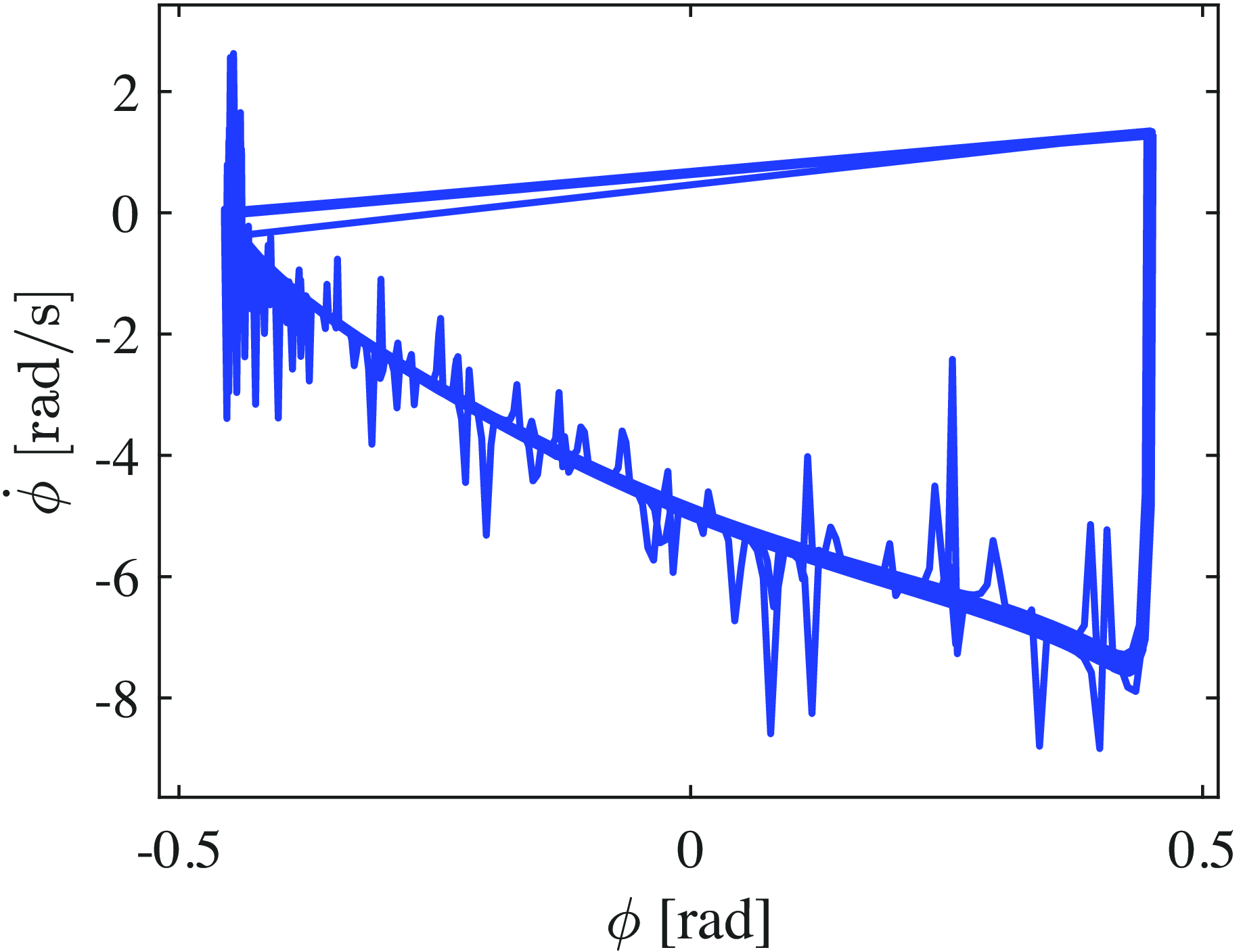
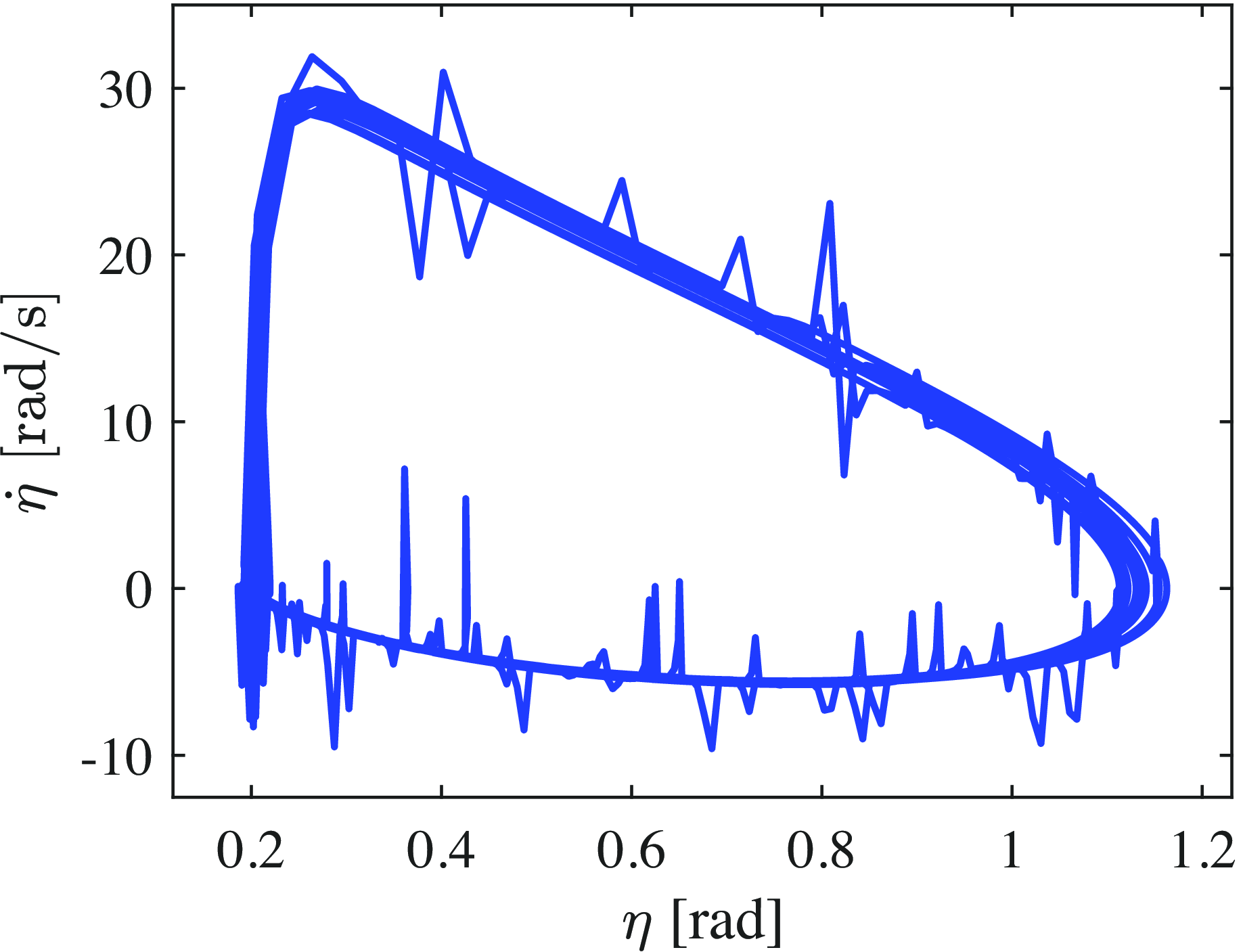
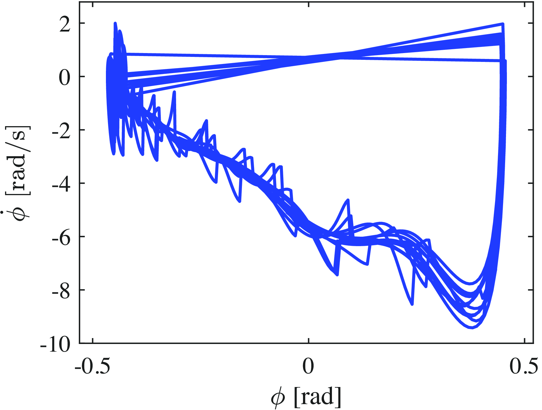
, and the actual values during steady-state walking using OZC, respectively. Immediately after the collision, the system deviates from the target trajectory but quickly converges back to it. Figures 19 and 20 show the phase diagrams of
 $\phi$
-
 $\dot {\phi }$
and
 $\eta$
-
 $\dot {\eta }$
, respectively, during steady-state OZC walking. These figures confirm the formation of a limit cycle. The average walking speed with this OZC-based approach was 0.829 m/s, and the SR value was 1.442.
Variations in
 $u_2$
during OZC-based walking with respect to time.

Variations in
 $\eta$
during OZC-based walking with respect to time.

Variations in
 $u_3$
during OZC-based walking with respect to time.

Variations in
 $\gamma$
during OZC-based walking with respect to time.

Variations in
 $u_1$
during OZC-based walking with respect to time.

Variations in the error between the target value (
 $\phi _d$
) and the actual value during OZC-based walking with respect to time.

Variations in the error between the target value (
 $\eta _d$
) and the actual value during OZC-based walking with respect to time.

Phase diagram of
 $\phi$
and
 $\dot {\phi }$
during steady-state OZC-based walking.

Phase diagram of
 $\eta$
and
 $\dot {\eta }$
during steady-state OZC-based walking.

4.2.2. NMPC-based walking
Subsequently, the walking performance using the proposed NMPC method was analyzed under the same conditions. Figures 21–28 show the time-dependent changes in
 $\theta _5$
,
 $u_4$
,
 $\phi$
,
 $u_2$
,
 $\eta$
,
 $u_3$
,
 $\gamma$
, and
 $u_1$
during NMPC-based steady-state walking under ideal environments, respectively. Evidently, NMPC-based walking also converges to the desired trajectory, similar to OZC. However, unlike the walking achieved with OZC, no spike-like torques are generated, and the torque transitions smoothly.
Variations in the torso angle during NMPC-based walking with respect to time.

Variations in
 $u_4$
during NMPC-based walking with respect to time.

Variations in
 $\phi$
during NMPC-based walking with respect to time.

Figures 29 and 30 show the errors between the target values,
 $\phi _d$
,
 $\eta _d$
, and the actual values during NMPC-based steady-state walking, respectively. As shown in these figures, the proposed NMPC-based walking demonstrates trajectory-tracking performance comparable to that with high-gain OZC, suggesting the potential feasibility of HZD-based trajectory optimization. Figures 31 and 32 show the phase diagrams of
 $\phi$
-
 $\dot {\phi }$
and
 $\eta$
-
 $\dot {\eta }$
, during NMPC-based steady-state walking, respectively. These figures indicate that a limit cycle is also formed during NMPC-based walking. The average walking speed with the NMPC-based method was 0.832 m/s, and the SR value was 1.177. Thus, the proposed walking method achieves a similar speed and convergence to the desired trajectory to OZC-based walking approach, while significantly improving energy efficiency.
Variations in
 $u_2$
during NMPC-based walking with respect to time.

Variations in
 $\eta$
during NMPC-based walking with respect to time.

Variations in
 $u_3$
during NMPC-based walking with respect to time.

Variations in
 $\gamma$
during NMPC-based walking with respect to time.

Variations in
 $u_1$
during NMPC-based walking with respect to time.

Variations in the error between the desired value (
 $\phi _d$
) and the actual value during NMPC-based walking with respect to time.

Variations in the error between the target value (
 $\eta _d$
) and the actual value during NMPC-based walking with respect to time.

Phase diagram of
 $\phi$
and
 $\dot {\phi }$
during NMPC-based steady-state walking.

Phase diagram of
 $\eta$
and
 $\dot {\eta }$
during NMPC-based steady-state walking.

4.3. Walking in an environment with disturbances
4.3.1. OZC-based walking in disturbances
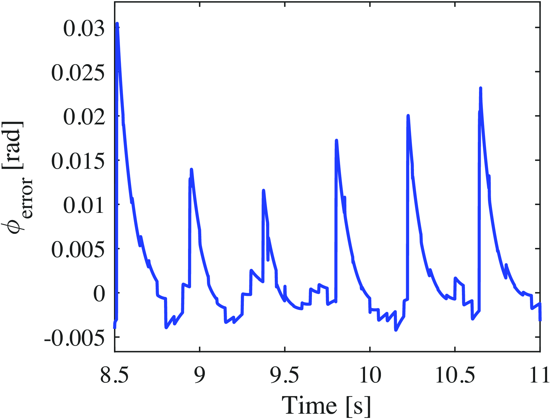
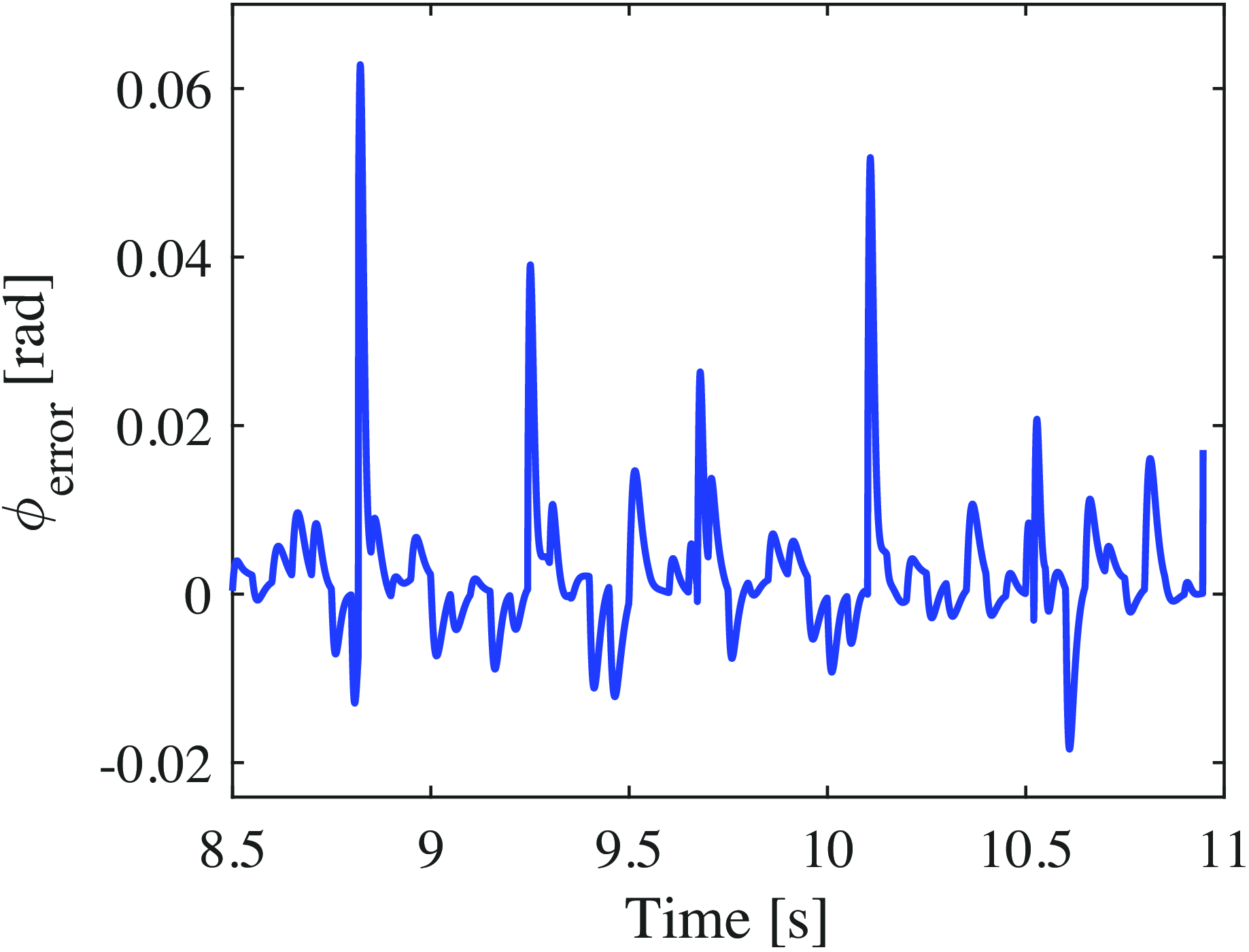
The previous analysis examined walking under ideal conditions without disturbances. This section evaluates walking performance in an environment with disturbances, which were modeled as random torques following a normal distribution (with the disturbance torque defined as 24 times the result of MATLAB’s randn function), applied to each joint for 1 ms every 50 ms. Figures 33–40 show the time-dependent changes in
 $\theta _5$
,
 $u_4$
,
 $\phi$
,
 $u_2$
,
 $\eta$
,
 $u_3$
,
 $\gamma$
, and
 $u_1$
during OZC-based steady-state walking in an environment with disturbances, respectively. Figures 41 and 42 show the errors between the target values,
 $\phi _d$
,
 $\eta _d$
, and the actual values during OZC-based steady-state walking in an environment with disturbances. Even in the presence of disturbances, high-gain OZC ensures strong tracking performance with the desired trajectory. However, the torque waveforms exhibit significant spikes, which are expected to considerably impact energy efficiency. Additionally, generating such large torques in practice is challenging, raising concerns about the feasibility of this approach. Figures 43 and 44 show the phase diagrams of
 $\phi$
-
 $\dot {\phi }$
and
 $\eta$
-
 $\dot {\eta }$
, during OZC-based steady-state walking under disturbances, respectively. Although the disturbances cause the robot’s state to deviate from the limit cycle, it quickly converges back to the original trajectory. The average walking speed for the OZC-based approach under disturbances was 0.829 m/s and the SR value was 1.979. While the walking speed is almost the same as when there are no disturbances, energy consumption increased substantially, leading to a significant reduction in energy efficiency.
Variations in the torso angle during OZC-based walking in disturbance environment with respect to time.

Variations in
 $u_4$
during OZC-based walking in disturbance environment with respect to time.

Variations in
 $\phi$
during OZC-based walking in disturbance environment with respect to time.

Variations in
 $u_2$
during OZC-based walking in disturbance environment with respect to time.

Variations in
 $\eta$
during OZC-based walking in disturbance environment with respect to time.

Variations in
 $u_3$
during OZC-based walking in disturbance environment with respect to time.

Variations in
 $\gamma$
during OZC-based walking in disturbance environment with respect to time.

Variations in
 $u_1$
during OZC-based walking in disturbance environment with respect to time.

Variations in the error between the desired value (
 $\phi _d$
) and the actual value during OZC-based walking in disturbance environment with respect to time.

4.3.2. NMPC-based walking in disturbances
Figures 45–52 show the time-dependent changes in
 $\theta _5$
,
 $u_4$
,
 $\phi$
,
 $u_2$
,
 $\eta$
,
 $u_3$
,
 $\gamma$
, and
 $u_1$
during NMPC-based steady-state walking in the disturbance environment, respectively. Figures 53 and 54 show the errors between the desired values,
 $\phi _d$
,
 $\eta _d$
, and the actual values during NMPC-based steady-state walking in the disturbance environment respectively. The proposed NMPC-based control achieves a level of convergence to the desired trajectory comparable to high-gain OZC. Additionally, no sharp torque spikes are observed, and the maximum torque values remain within realistic limits. Figures 55 and 56 show the phase diagrams for
 $\phi$
-
 $\dot {\phi }$
and
 $\eta$
-
 $\dot {\eta }$
during NMPC-based steady-state walking under disturbances, respectively. Although the disturbances cause the robot’s state to deviate from the trajectory, the state gradually converges back to the original trajectory, unlike in the case of OZC-based walking. The average walking speed using the NMPC-based control was 0.834 m/s and the SR value was 1.287. In conventional OZC-based walking, energy efficiency significantly deteriorates in disturbed environments. However, the proposed NMPC-based walking substantially mitigates this issue.
Variations in the error between the target value (
 $\eta _d$
) and the actual value during OZC-based walking in disturbance environment with respect to time.

Phase diagram of
 $\phi$
and
 $\dot {\phi }$
for OZC-based steady-state walking in disturbance environment.

Phase diagram of
 $\eta$
and
 $\dot {\eta }$
for OZC-based steady-state walking in disturbance environment.

Walking performance.

Variations in the torso angle during NMPC-based walking in disturbance environment with respect to time.

Variations in
 $u_4$
during NMPC-based walking in disturbance environment with respect to time.

Variations in
 $\phi$
during NMPC-based walking in disturbance environment with respect to time.

Variations in
 $u_2$
during NMPC-based walking in disturbance environment with respect to time.

Variations in
 $\eta$
during NMPC-based walking in disturbance environment with respect to time.

4.4. Overall comparison
To measure the computation time of NMPC and OZC, the original MATLAB programs were converted to C using MEX files, and the computation time per input was evaluated. The average computation times were approximately 0.32 ms for NMPC and 0.026 ms for OZC. Although the computation time for NMPC is longer than that of OZC, it remains practical even for fast robot control cycles (approximately 1 ms). The results are summarized in Table III. Therefore, the proposed NMPC-based method achieved a walking speed and convergence to the desired trajectory nearly identical to that of the OZC-based approach, with a significant improvement in energy efficiency, particularly in the disturbed environment.
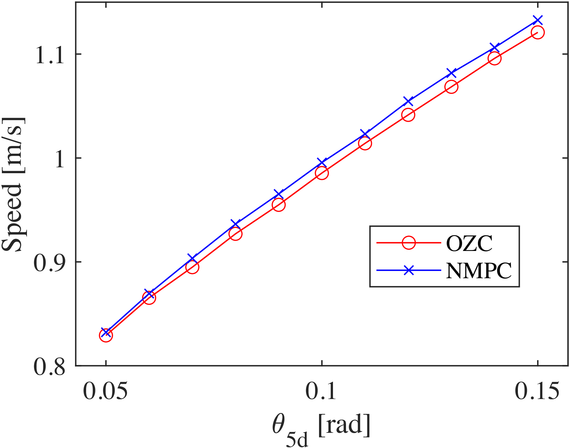
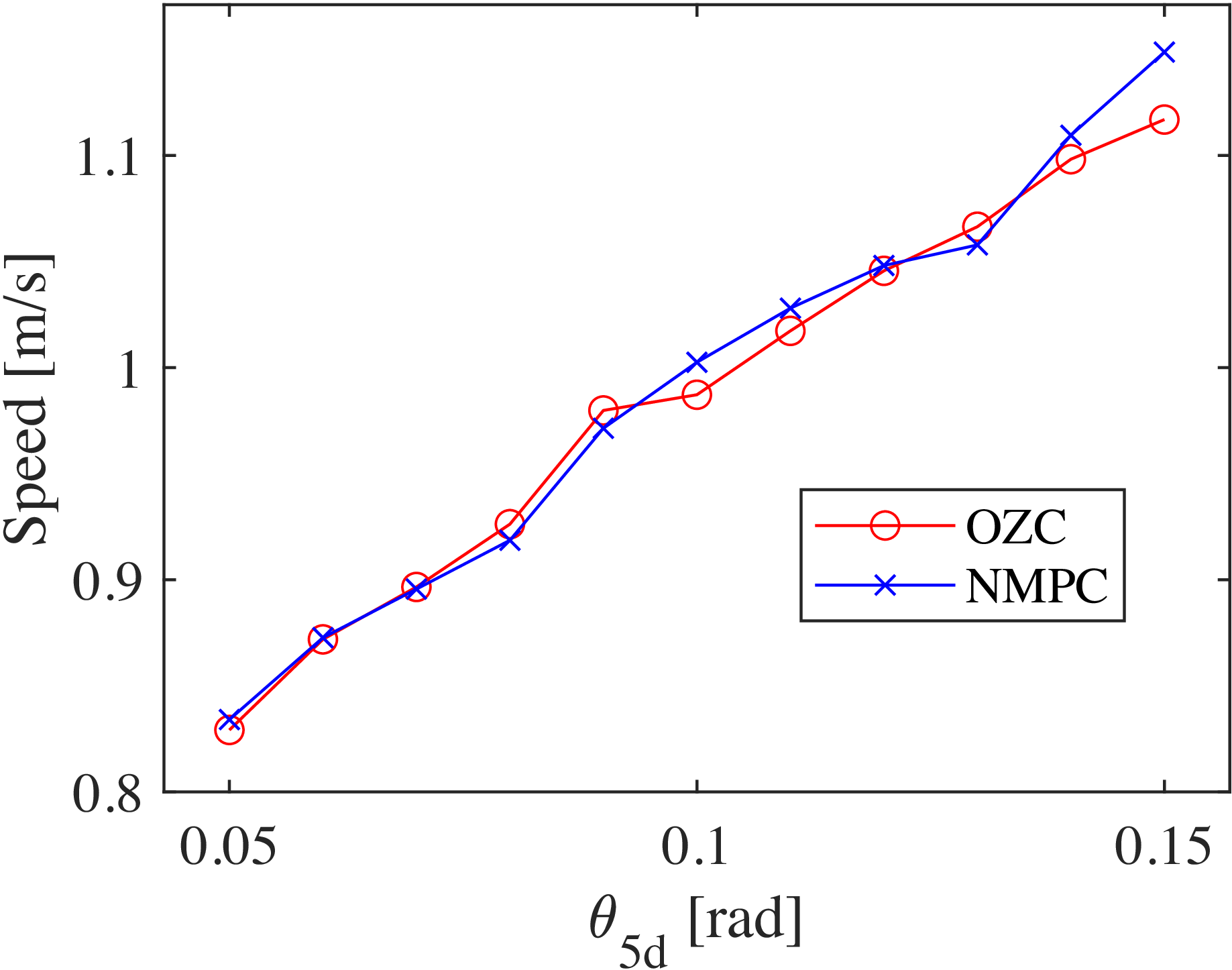
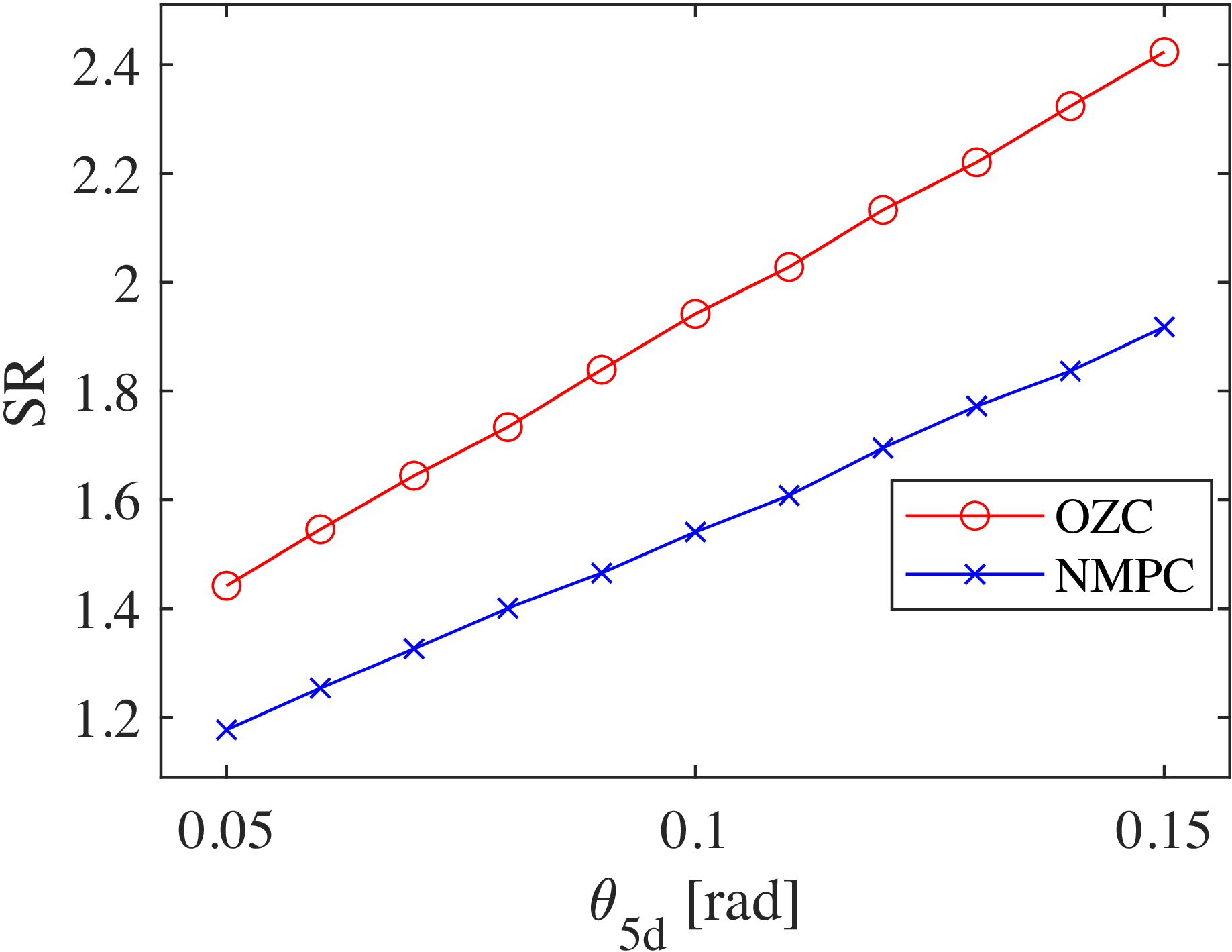
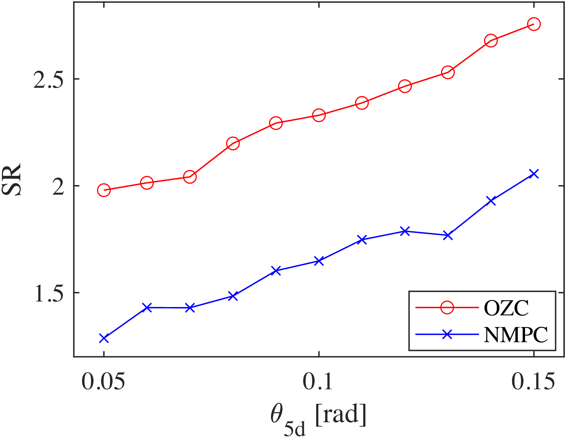
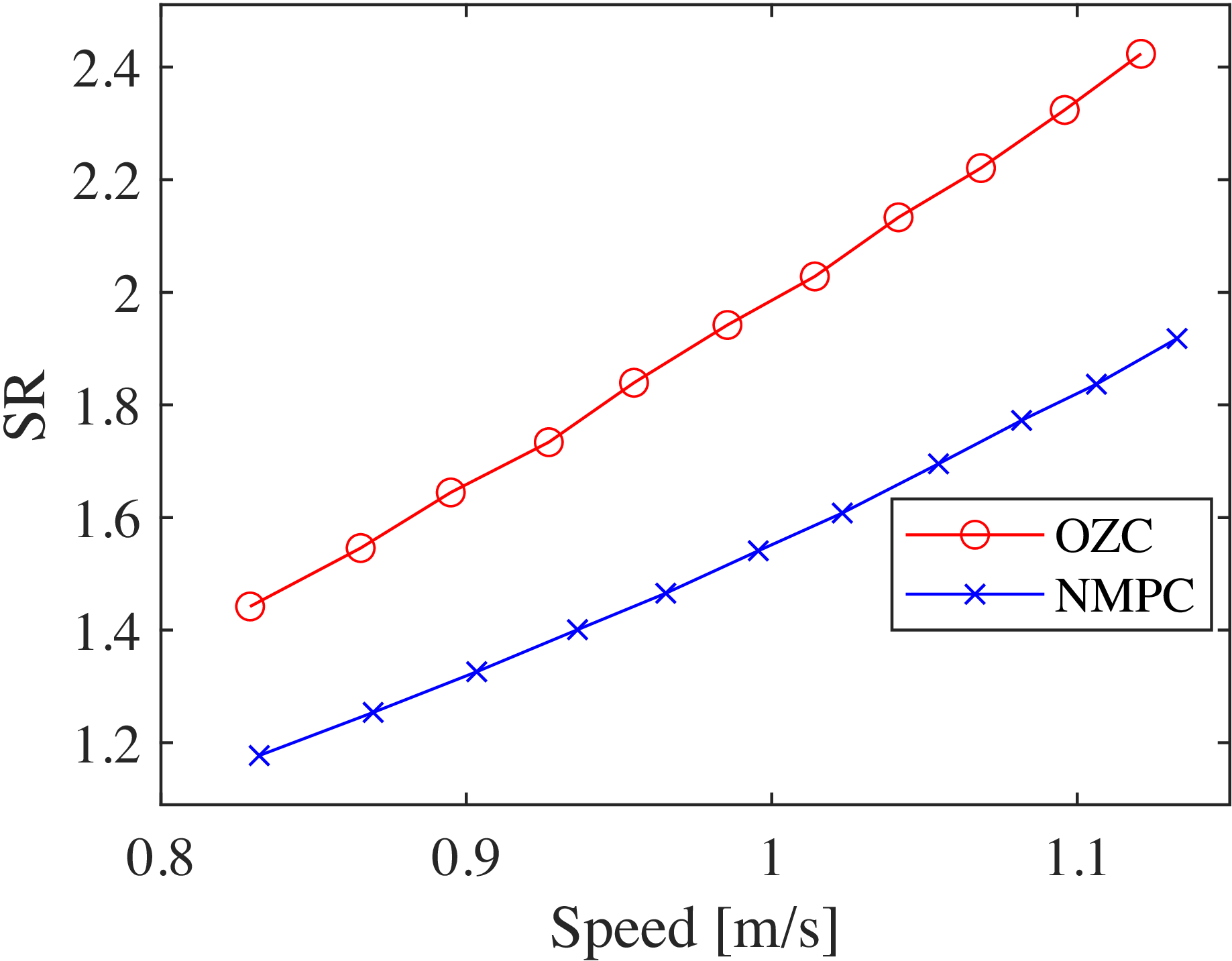
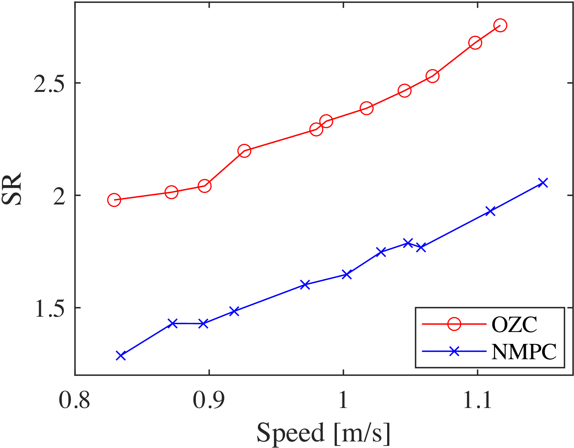
Furthermore, Figures 57 and 58 show the walking speeds of OZC and NMPC-based walking under conditions without and with disturbances when the desired torso angle is varied. Figures 59 and 60 present the SR of OZC and NMPC-based walking with respect to the desired torso angle in these conditions. Additionally, Figures 61 and 62 show the SR of OZC and NMPC-based walking with respect to the walking speed in these conditions. It can be observed that the walking speeds of OZC and NMPC remain similar at the same desired torso angle, regardless of the presence of disturbances. However, the SR values of NMPC are consistently lower than those of OZC for all desired torso angles (or the walking speed according to the torso angles), with this trend becoming more pronounced in the presence of disturbances. Therefore, the proposed method achieves energy-efficient walking not only locally but also in terms of global walking speed.
Variations in
 $u_3$
during NMPC-based walking in disturbance environment with respect to time.

Variations in
 $\gamma$
during NMPC-based walking in disturbance environment with respect to time.

Variations in
 $u_1$
during NMPC-based walking in disturbance environment with respect to time.

Variations in the error between the desired value (
 $\phi _d$
) and the actual value during NMPC-based walking in disturbance environment with respect to time.

Variations in the error between the target value (
 $\eta _d$
) and the actual value during NMPC-based walking in disturbance environment with respect to time.

Phase diagram of
 $\phi$
and
 $\dot {\phi }$
for NMPC-based steady-state walking in disturbance environment.

Phase diagram of
 $\eta$
and
 $\dot {\eta }$
for NMPC-based steady-state walking in disturbance environment.

Walking speeds for OZC and NMPC steady-state walking with respect to
 $\theta _{5d}$
.

Walking speeds for OZC and NMPC steady-state walking in disturbance environment with respect to
 $\theta _{5d}$
.

SR values for OZC and NMPC steady-state walking with respect to
 $\theta _{5d}$
.

SR values for OZC and NMPC steady-state walking in disturbance environment with respect to
 $\theta _{5d}$
.

SR values for OZC and NMPC steady-state walking with respect to walking speed.

SR values for OZC and NMPC steady-state walking in disturbance environment with respect to walking speed.

5. Conclusion and future works
This paper presented an NMPC-based method for generating limit cycles suitable for bipedal walking, and the mechanism for generating limit cycles was explained in detail. Specifically, it uses the proposed NMPC to attract the robot’s state to a virtual constraint trajectory based on the support leg angle. To demonstrate the effectiveness of the proposed method, numerical simulations were conducted to compare it with the conventional OZC method. The results showed that the proposed method not only exhibits convergence to the desired trajectory similar to the conventional method but also offers significant advantages in terms of energy efficiency. In particular, our approach demonstrated substantial improvements in environments with disturbances, successfully mitigating their impact on energy efficiency. Additionally, the computation time required by the proposed method was analyzed, and it was confirmed that the calculations can be performed within a practical control cycle. Although this study did not explore trajectory optimization, the convergence to the target trajectory was comparable to that of high-gain OZC, suggesting that HZD-based optimization is feasible. Therefore, future work will focus on trajectory optimization using HZD and extension of the method to three-dimensional walking by incorporating coronal plane motions.
Supplementary material
The supplementary material for this article can be found at https://doi.org/10.1017/S0263574725103020.
Author contributions
Y. Hanazawa conceived and designed this study. Y. Hanazawa and Y. Uchino verified the effectiveness of the proposed method. Y. Hanazawa wrote the article. S. Sagara provided technical support for the study.
Financial support
Not support.
Competing interest
The authors declare no conflicts of interest.
Use of AI-assisted tools
The authors used Claude Sonnet 4.5 only for English language editing to improve readability.
Ethical approval
Not applicable.
Appendix
Details of the model
The components of matrices
 $\boldsymbol{M}(\boldsymbol{q})$
,
 $\boldsymbol{C}(\boldsymbol{q}, \dot {\boldsymbol{q}})$
, and
 $\boldsymbol{G}(\boldsymbol{q})$
are as follows, where
 $\boldsymbol{H}(\boldsymbol{q},\dot {\boldsymbol{q}}) = \boldsymbol{C}(\boldsymbol{q}, \dot {\boldsymbol{q}}) + \boldsymbol{G}(\boldsymbol{q})$
,
 $M_{cij}$
denotes the
 $(i,j)$
-th component of
 $\boldsymbol{M}(\boldsymbol{q})$
,
 $C_{ci}$
denotes the
 $i$
-th row component of
 $\boldsymbol{C}(\boldsymbol{q}, \dot {\boldsymbol{q}})$
, and
 $G_{ci}$
denotes the
 $i$
-th row component of
 $\boldsymbol{G}(\boldsymbol{q})$
.
 \begin{align*} M_{c11} &= I_1 + a_1^2 m_1 + l_1^2 m_1 + 2 l_1^2 m_2 + l_1^2 m_3 + l_1^2 m_h \\ M_{c12} &= l_1 \cos (\theta _1 - \theta _2) (a_2 m_2 + l_2 m_1 + l_2 m_2 + l_2 m_3 + l_2 m_h) \\ M_{c13} &= - l_1 \cos (\theta _1 - \theta _3) (b_2 m_2 + l_2 m_1) \\ M_{c14} &= - b_1 l_1 m_1 \cos (\theta _1 - \theta _4) \\ M_{c15} &= a_3 l_1 m_3 \cos (\theta _1 - \theta _5) \\ M_{c21} &= l_1 \cos (\theta _1 - \theta _2) (a_2 m_2 + l_2 m_1 + l_2 m_2 + l_2 m_3 + l_2 m_h) \\ M_{c22} &= I_2 + a_2^2 m_2 + l_2^2 m_1 + l_2^2 m_2 + l_2^2 m_3 + l_2^2 m_h \\ M_{c23} &= - l_2 \cos (\theta _2 - \theta _3) (b_2 m_2 + l_2 m_1) \\ M_{c24} &= - b_1 l_2 m_1 \cos (\theta _2 - \theta _4) \\ M_{c25} &= a_3 l_2 m_3 \cos (\theta _2 - \theta _5) \\ M_{c31} &= - l_1 \cos (\theta _1 - \theta _3) (b_2 m_2 + l_2 m_1) \\ M_{c32} &= - l_2 \cos (\theta _2 - \theta _3) (b_2 m_2 + l_2 m_1) \\ M_{c33} &= I_2 + b_2^2 m_2 + l_2^2 m_1 \\ M_{c34} &= b_1 l_2 m_1 \cos (\theta _3 - \theta _4) \\ M_{c35} &= 0 \\ M_{c41} &= - b_1 l_1 m_1 \cos (\theta _1 - \theta _4) \\ M_{c42} &= - b_1 l_2 m_1 \cos (\theta _2 - \theta _4) \\ M_{c43} &= b_1 l_2 m_1 \cos (\theta _3 - \theta _4) \\ M_{c44} &= I_1 + b_1^2 m_1 \\ M_{c45} &= 0 \\ M_{c51} &= a_3 l_1 m_3 \cos (\theta _1 - \theta _5) \\ M_{c52} &= a_3 l_2 m_3 \cos (\theta _2 - \theta _5) \\ M_{c53} &= 0 \\ M_{c54} &= 0 \\ M_{c55} &= I_3 + a_3^2 m_3\\ C_{c1} &= l_1 ( a_2 \dot {\theta }_2^2 m_2 \sin (\theta _1 - \theta _2) + a_3 \dot {\theta }_5^2 m_3 \sin (\theta _1 - \theta _5) - b_1 \dot {\theta }_4^2 m_1 \sin (\theta _1 - \theta _4) - b_2 \dot {\theta }_3^2 m_2 \sin (\theta _1 - \theta _3) \\ &+ \dot {\theta }_2^2 l_2 m_1 \sin (\theta _1 - \theta _2) + \dot {\theta }_2^2 l_2 m_2 \sin (\theta _1 - \theta _2) + \dot {\theta }_2^2 l_2 m_3 \sin (\theta _1 - \theta _2) \\ &- \dot {\theta }_3^2 l_2 m_1 \sin (\theta _1 - \theta _3) + \dot {\theta }_2^2 l_2 m_h \sin (\theta _1 - \theta _2) )\\ C_{c2} &= a_3 \dot {\theta }_5^2 l_2 m_3 \sin (\theta _2 - \theta _5) - a_2 \dot {\theta }_1^2 l_1 m_2 \sin (\theta _1 - \theta _2) - \dot {\theta }_3^2 l_2^2 m_1 \sin (\theta _2 - \theta _3) - b_1 \dot {\theta }_4^2 l_2 m_1 \sin (\theta _2 - \theta _4) \\ &- b_2 \dot {\theta }_3^2 l_2 m_2 \sin (\theta _2 - \theta _3) - \dot {\theta }_1^2 l_1 l_2 m_1 \sin (\theta _1 - \theta _2) - \dot {\theta }_1^2 l_1 l_2 m_2 \sin (\theta _1 - \theta _2) \\ &- \dot {\theta }_1^2 l_1 l_2 m_3 \sin (\theta _1 - \theta _2) - \dot {\theta }_1^2 l_1 l_2 m_h \sin (\theta _1 - \theta _2) \end{align*}
 \begin{align*} C_{c3} &=\dot {\theta }_2^2 l_2^2 m_1 \sin (\theta _2 - \theta _3) + b_2 \dot {\theta }_1^2 l_1 m_2 \sin (\theta _1 - \theta _3) + b_2 \dot {\theta }_2^2 l_2 m_2 \sin (\theta _2 - \theta _3) \\ &+ b_1 \dot {\theta }_4^2 l_2 m_1 \sin (\theta _3 - \theta _4) + \dot {\theta }_1^2 l_1 l_2 m_1 \sin (\theta _1 - \theta _3) \\ C_{c4} &= b_1 m_1 ( \dot {\theta }_1^2 l_1 \sin (\theta _1 - \theta _4) + \dot {\theta }_2^2 l_2 \sin (\theta _2 - \theta _4) - \dot {\theta }_3^2 l_2 \sin (\theta _3 - \theta _4) ) \\ C_{c5} &= - a_3 m_3 ( \dot {\theta }_1^2 l_1 \sin (\theta _1 - \theta _5) + \dot {\theta }_2^2 l_2 \sin (\theta _2 - \theta _5) )\\ G_{c1} &= -g \sin {\theta _1} (a_1 m_1 + l_1 m_1 + 2 l_1 m_2 + l_1 m_3 + l_1 m_h) \\ G_{c2} &= -g \sin {\theta _2} (a_2 m_2 + l_2 m_1 + l_2 m_2 + l_2 m_3 + l_2 m_h) \\ G_{c3} &= g \sin {\theta _3} (b_2 m_2 + l_2 m_1) \\ G_{c4} &= b_1 m_1 \sin {\theta _4} g \\ G_{c5} &= - a_3 m_3 \sin {\theta _5} g \end{align*}