





No CrossRef data available.
Article contents
Simulating exploration versus exploitation in agent foraging under different environment uncertainties
Published online by Cambridge University Press: 19 March 2019
Abstract
For artificial agents trading off exploration (food seeking) versus (short-term) exploitation (or consumption), our experiments suggest that uncertainty (interpreted information, theoretically) magnifies food seeking. In more uncertain environments, with food distributed uniformly randomly, exploration appears to be beneficial. In contrast, in biassed (less uncertain) environments, with food concentrated in only one part, exploitation appears to be more advantageous. Agents also appear to do better in biassed environments.
Information
- Type
- Open Peer Commentary
- Information
- Copyright
- Copyright © Cambridge University Press 2019
References
Bartumeus, F., Campos, D., Ryu, W. S., Lloret-Cabot, R., Méndez, V. & Catalan, J. (2016) Foraging success under uncertainty: Search tradeoffs and optimal space use. Ecology Letters 19(11):1299–313.Google Scholar
Boulton, D. M. & Wallace, C. S. (1969) The information content of a multistate distribution. Journal of Theoretical Biology 23:269–78.Google Scholar
Chmait, N., Dowe, D. L., Green, D. G. & Li, Y. F. (2015) Observation, communication and intelligence in agent-based systems. In: 8th International Conference on Artificial General Intelligence, ed. Bieger, J., Goertzel, B., & Potapov, Alexey, pp. 50–59. Lecture Notes in Computer Science 9205. Springer.Google Scholar
Chmait, N., Dowe, D. L., Li, Y. F. & Green, D. G. (2017) An information-theoretic predictive model for the accuracy of AI agents adapted from psychometrics. In: 10th International Conference on Artificial General Intelligence, ed. Everitt, T., Goertzel, B. & Potapov, A., pp. 225–36. Lecture Notes in Artificial Intelligence and Lecture Notes in Bioinformatics 10414. Springer.Google Scholar
Chmait, N., Dowe, D. L., Li, Y. F., Green, D. G. & Insa-Cabrera, J. (2016a) Factors of collective intelligence: How smart are agent collectives? In: European 22nd Conference on Artificial Intelligence, ed. Kaminka, G. A., Fox, M., Bouquet, P., Hüllermeier, E., Dignum, V., Dignum, F. & van Harmelen, F., pp. 542–50. IOS Press.Google Scholar
Chmait, N., Li, Y. F., Dowe, D. L. & Green, D. G. (2016b) A dynamic intelligence test framework for evaluating AI agents. In: Proceedings of 1st International Workshop on Evaluating General-Purpose AI (EGPAI 2016), A workshop held in conjunction with the European Conference on Artificial Intelligence (ECAI 2016), The Hague, The Netherlands.Google Scholar
Green, D. G., Klomp, N., Rimmington, G. & Sadedin, S. (2006) Complexity in landscape ecology, vol. 4. Springer Science & Business Media.Google Scholar
Green, D. G., Liu, J. & Abbass, H. A. (2014) Dual-phase evolution (chapter 1). In: Dual phase evolution, ed. Green, D. G., Liu, J. & Abbass, H. A., pp. 3–40. Springer.Google Scholar
Hernández-Orallo, J., Baroni, M., Bieger, J., Chmait, N., Dowe, D. L., Hofmann, K., Martínez-Plumed, F., Strannegård, C. & Thórisson, K. R. (2017) A new AI evaluation cosmos: Ready to play the game? AI Magazine 38(3):66–69.Google Scholar
Mehlhorn, K., Newell, B. R., Todd, P. M., Lee, M. D., Morgan, K., Braithwaite, V. A., Hausmann, D., Fiedler, K. & Gonzalez, C. (2015) Unpacking the exploration–exploitation tradeoff: A synthesis of human and animal literatures. Decision 2(3):191.Google Scholar
Newman, M. E. J. & Ziff, R. M. (2000) Efficient Monte-Carlo algorithm and high-precision results for percolation. Physical Review Letters 85(19):4104–107.Google Scholar
Paperin, G., Green, D. G. & Sadedin, S. (2011) Dual-phase evolution in complex adaptive systems. Journal of the Royal Society Interface 8(58):609–29.Google Scholar
Wallace, C. S. & Dowe, D. L. (1999) Minimum message length and Kolmogorov complexity. Computer Journal 42(4):270–83.Google Scholar
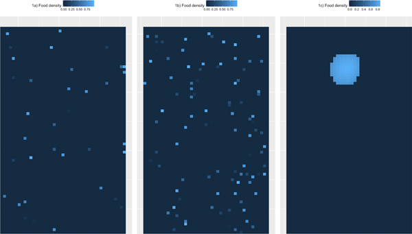
Figure 1. Examples of possible environments with different distributions and percentages of rewards (food) and reward densities. The first two plots (1a and 1b) show rewards distributed uniformly randomly across the environment (with food more abundant in environment 1b), whereas plot 1c (on the right) has a biassed distribution of food that is concentrated in one part of the environment.
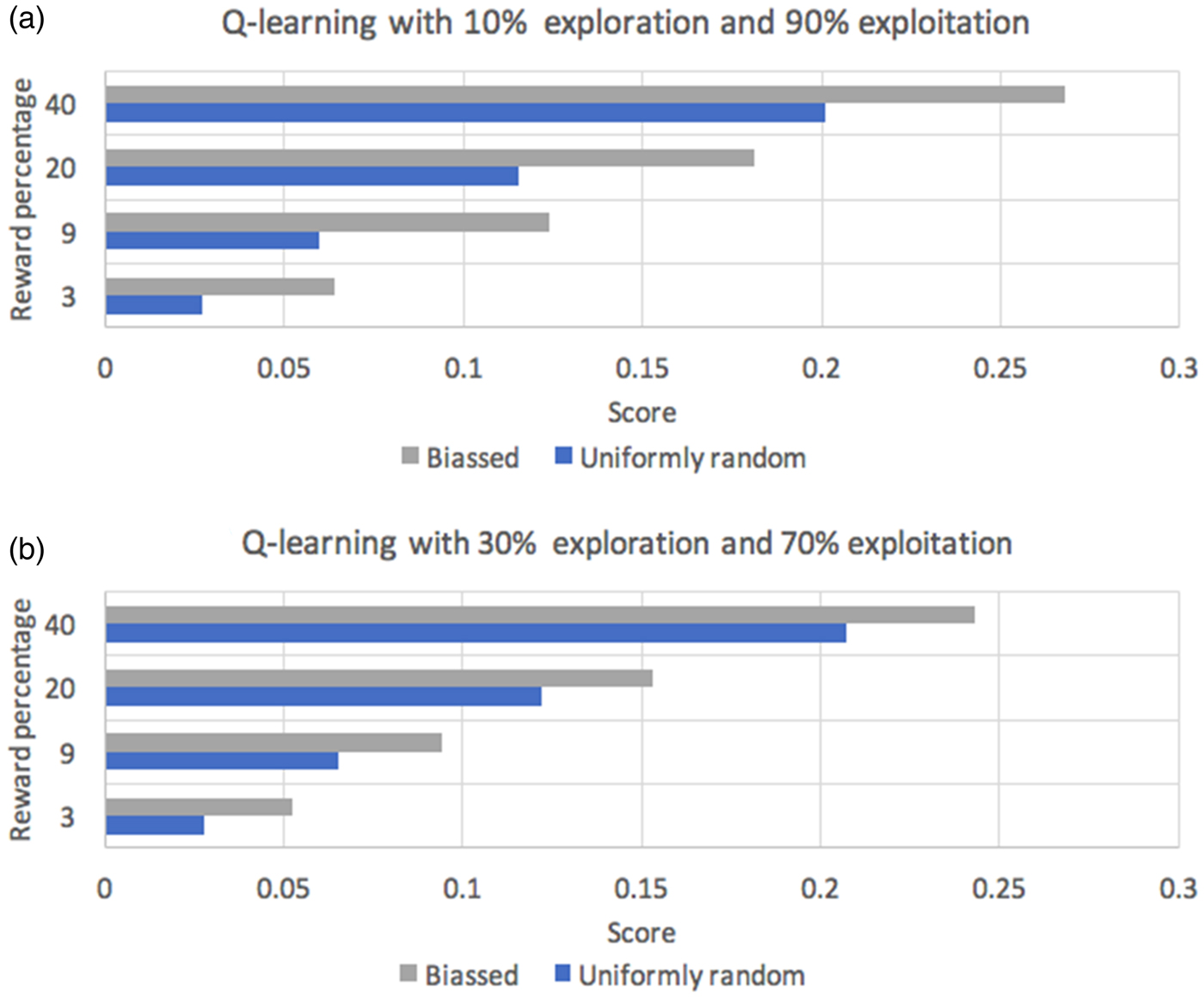
Figure 2. Q-Learning algorithm scores in environments with different percentages of biassed and uniformly random distributed food across the environment space.
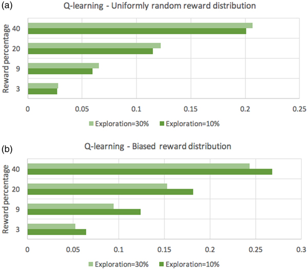
Figure 3. Q-learning agent behaviour under different exploration-exploitation trade-offs in biassed and uniformly random reward-distributed environments.
Target article
Related commentaries (22)
Beyond “incentive hope”: Information sampling and learning under reward uncertainty
Random isn't real: How the patchy distribution of ecological rewards may generate “incentive hope”
We simulate the behaviour of artificial agents foraging for food in toroidal environments consisting of 400×400 cells, over 10,000 repeated experiments, each consisting of 300 iterations or sequences of observation-action-reward, similar to the architecture described by Chmait et al. (Reference Chmait, Dowe, Green, Li, Bieger, Goertzel and Potapov2015; Reference Chmait, Dowe, Li, Green, Insa-Cabrera, Kaminka, Fox, Bouquet, Hüllermeier, Dignum, Dignum and van Harmelen2016a; Reference Chmait, Li, Dowe and Green2016b). This number of iterations makes it possible for artificial agents to discover a fraction of the environment space, and therefore this number of iterations models the agents’ short-term foraging behaviour. Rewards in the range [0,1] can have different spatial distributions (Fig. 1). A cell reward of 0 indicates unavailability of food in that cell, whereas food density is maximum at 1.
Examples of possible environments with different distributions and percentages of rewards (food) and reward densities. The first two plots (1a and 1b) show rewards distributed uniformly randomly across the environment (with food more abundant in environment 1b), whereas plot 1c (on the right) has a biassed distribution of food that is concentrated in one part of the environment.
Agents can only see their eight neighbouring cells (equivalently, a Moore's neighbourhood with n = 1), allowing for more flexible navigation across the environment in comparison to Anselme & Güntürkün (A&G). In each experiment, agents are initialized with different starting cell positions and evaluated in environments comprising different percentages of food. At any time step, we arbitrarily assume that an agent eats 0.1 worth of reward once it lands on a cell that contains ≥0.1 food reward. An agent's score is calculated as its average reward over the 300 iterations. To mimic natural environments, we introduce some stochasticity by allowing environment cells, with a very low probability, to gradually produce or deplete food. When the food resources are uniformly randomly distributed (e.g., Figs. 1a and 1b), the uncertainty of an environment with food distribution probability p will – by symmetry – be equal to that of an environment with food distribution probability (1 − p) (Boulton & Wallace, Reference Boulton and Wallace1969). As such, we will only experiment with environments with p ≤ 0.5.
Efficient foraging requires a trade-off between two operations (Bartumeus et al. Reference Bartumeus, Campos, Ryu, Lloret-Cabot, Méndez and Catalan2016; Mehlhorn et al. Reference Mehlhorn, Newell, Todd, Lee, Morgan, Braithwaite, Hausmann, Fiedler and Gonzalez2015): exploration, which aims to locate resources, and exploitation, which aims to maximize the amount gathered from each resource. These two operations can occur in separate phases (Green et al. Reference Green, Liu, Abbass, Green, Liu and Abbass2014; Paperin et al. Reference Paperin, Green and Sadedin2011) and require a balance between the time allocated to each. The percentage of resources in the landscape is crucial to the above trade-off.
We note in passing that, if cells are arranged in a two-dimensional grid, with a random scatter of cells containing resources, then there is a critical percolation density ~0.592746 (Newman & Ziff Reference Newman and Ziff2000) above which most of the resource cells become connected into a single “giant component” (Green et al. Reference Green, Klomp, Rimmington and Sadedin2006; Reference Green, Liu, Abbass, Green, Liu and Abbass2014; Paperin et al. Reference Paperin, Green and Sadedin2011). That is, when ~59% of cells contain resources, a phase change occurs and the resource transforms from being random, scattered items to a single, connected resource.
In our experiments, a reinforcement Q-learning algorithm was evaluated under different exploration-exploitation trade-offs across environments with biassed and uniformly randomly distributed food. Our Q-learning agents learn an action-selection policy where an action consists of taking a step in any of the possible directions, leading into one of the neighbouring cells (Chmait et al. Reference Chmait, Dowe, Li, Green, Insa-Cabrera, Kaminka, Fox, Bouquet, Hüllermeier, Dignum, Dignum and van Harmelen2016a; Reference Chmait, Li, Dowe and Green2016b).
Results illustrated in Figure 2 (both 2a and 2b) suggest that Q-learning performs better in environments with biassed reward distributions, even when relatively abundant with food (e.g., 40% of cells contain some density of food). In such cases, a Q-learning algorithm seems to better learn a policy (or the sequence of actions) leading to the food source, and then spends time exploiting rewards around this source.
Q-Learning algorithm scores in environments with different percentages of biassed and uniformly random distributed food across the environment space.
We now suggest this to be perhaps a special case of something more general in terms of (algorithmic) information theory. If we encode environment cell-rewards as a vector of 0's and 1's denoting the availability and absence of food in these cells, respectively, we expect the agents’ scores to be lower in environments of high Solomonoff-Kolmogorov complexities (Boulton & Wallace Reference Boulton and Wallace1969; Wallace & Dowe Reference Wallace and Dowe1999), even across different percentages of reward in the environment.
Noteworthy is that the ratio of the scores (of the biassed divided by the uniformly random distributions of rewards) in Figure 2 (both a and b) seems to be monotonically decreasing with the percentage of food available in the environment, giving a bigger ratio in a food-scarce environment. For instance, in an environment space similar to that depicted in Figures 1a and (especially) 1b, reward patterns are seemingly of high randomness relative to environment spaces similar to that in Figure 1c. Thus, as the reward pattern becomes closer to (uniformly) random, learning seems of less importance/relevance to the agent's score. Nevertheless, further controlled experimentation is required to assess the above premise, across different food-density distributions (under 50%), time periods (long-term behaviour) and types of foraging agents (among other factors) (Chmait et al. Reference Chmait, Dowe, Li, Green, Insa-Cabrera, Kaminka, Fox, Bouquet, Hüllermeier, Dignum, Dignum and van Harmelen2016a; Reference Chmait, Dowe, Li, Green, Everitt, Goertzel and Potapov2017; Hernández-Orallo et al. Reference Hernández-Orallo, Baroni, Bieger, Chmait, Dowe, Hofmann, Martínez-Plumed, Strannegård and Thórisson2017). Moreover, in multiagent foraging, the trade-off can involve balancing the allocation of agents to exploration and exploitation.
Figure 3 illustrates the same results as in Figure 2, but instead contrasts the Q-learning agent scores under different exploration-exploitation trade-offs. We observe that, when food is uniformly randomly distributed across the environment space (in turn making the environment of higher uncertainty), more exploration of the environment (food seeking) seems to increase an agent's overall food. This is in contrast to environments where food is concentrated in only one part (lower uncertainty, e.g., Figure 1c), in which more exploitation was beneficial, and exploring different portions of the environment diverted the agents from the only consistent food source available.
Q-learning agent behaviour under different exploration-exploitation trade-offs in biassed and uniformly random reward-distributed environments.
The contrast between Figures 3a and 3b supports the hypothesis of A&G that uncertainty magnifies food seeking.