1 Introduction
After the initial development of fuzzy set theory [Reference Zadeh38, Reference Zadeh39], there have been several new concepts proposed for more advanced fuzzy sets like picture fuzzy set [Reference Singh and Kumar28], extended picture fuzzy set or type-2 picture fuzzy set [Reference Singh and Kumar30], neutrosophic fuzzy set [Reference Singh and Kumar31], complex fuzzy set [Reference Singh and Kumar32], interval-valued fuzzy set [Reference Singh and Kumar29], and so forth. Among these, Atanassov [Reference Atanassov3] expanded this concept to intuitionistic fuzzy sets, which provide a flexible tool to address resistance arising from ambiguity and incorrect information. Two characteristic functions are used to represent the membership degree (
 $\mathcal {M}_D$
) and nonmembership degree (
 $\mathcal {N}_D$
) of universe elements to the intuitionistic fuzzy sets. Thus,
 $\mathcal {M}_D$
and
 $\mathcal {N}_D$
form intuitionistic fuzzy sets. Because this idea naturally occurs in real-world human language and behaviour, Psychology, alongside the other social science disciplines, has studied and used it extensively. Even so, fuzzy and intuitionistic fuzzy sets have been implemented to explain uncertainty-related real-world issues [Reference Singh and Kumar26]. However, there are instances in which a counter property is necessary to describe an object’s information that corresponds to an attribute. Zhang [Reference Zhang41] introduced bipolar fuzzy
 $(\mathcal {B}^{\mathcal {F}})$
sets to address these problems, which is an extension of the fuzzy sets. In
 $\mathcal {B}^{\mathcal {F}}$
-sets, the
 $\mathcal {M}_D$
lies in the interval
 $[-1, 1]$
. Every element in
 $\mathcal {B}^{\mathcal {F}}$
-sets are mixed with two values. One value denotes the fuzzy set’s particular property and lies in the interval
 $[0, 1]$
. The other one lies in the interval
 $[-1, 0]$
and denotes the degree to which a counter-property of the relevant fuzzy set is satisfied.
 $\mathcal {B}^{\mathcal {F}}$
-sets appear to have been investigated and used rather more frequently and passionately in recent years. Singh [Reference Singh33] stated that every day of our lives uses bipolar information, which is used to measure the information. The rationale is that binary values (0 and 1) do not correspond to the fundamental units of the human mind. Human cognition often uses the boundaries of the information to choose what parts of it to accept and reject [Reference Pandey, Ojha, Singh, Singh, Dwivedi and Bergey19]. According to Pedrycz and Chen [Reference Pedrycz and Chen20], bipolarity is an inevitable situation that deals with ambiguity and uncertainty in fuzzy characteristics and varies at each stage of time. Bipolar information may generally be categorized as pass or fail (True or False). As per Dubois and Prade’s report [Reference Dubois and Prade7], the primary factor is the simultaneous existence of these two areas in the specified
 $\mathcal {B}^{\mathcal {F}}$
-regions
 $[-1,0) \times (0, 1]$
. In this instance, processing the bipolar requests while simultaneously identifying the positive or negative areas is a difficult task [Reference Delgado, Marín, Pérez and Vila6]. The cause is bipolarity, which can have varying definitions depending on the stage of life. It is preferable to depict them using
 $\mathcal {B}^{\mathcal {F}}$
-properties. The positive
 $\mathcal {M}_D$
of a
 $\mathcal {B}^{\mathcal {F}}$
-set denotes a degree of partial attribute fulfilment, whereas the negative
 $\mathcal {M}_D$
denotes an implicit counter characteristic. In decision science, the
 $\mathcal {B}^{\mathcal {F}}$
-set is a sophisticated method for managing uncertainty.
Zhang and Zhang [Reference Zhang and Zhang44] gave YinYang bipolar logic and logical reasoning in the
 $\mathcal {B}^{\mathcal {F}}$
-framework. Zhang et al. [Reference Zhang, Zhang, Shi and Chen43] extended the YinYang bipolar logic proposed by Zhang and Zhang [Reference Zhang and Zhang44] into bipolar linaer algebra and YinYang-N-element cellular networks in a
 $\mathcal {B}^{\mathcal {F}}$
-framework. The problems related to neurobiological data mining, diagnostic analysis and psychiatric disorder classification were studied by Zhang et al. [Reference Zhang, Pandurangi, Peace, Zhang and Zhao42] by using vector machine in the
 $\mathcal {B}^{\mathcal {F}}$
-framework. The regulation of collective emotions in any organisation was studied in the
 $\mathcal {B}^{\mathcal {F}}$
-framework by Fink and Yolles [Reference Fink and Yolles8]. Wei et al. [Reference Wei, Alsaadi, Hayat and Alsaedi36] proposed hesitant
 $\mathcal {B}^{\mathcal {F}}$
-weighted geometric and averaging operators, and applied them to MADM (multi-attribute decision-making). Some
 $\mathcal {B}^{\mathcal {F}}$
-Hamacher aggregation operators were designed by Wei et al. [Reference Wei, Alsaadi, Hayat and Alsaedi37]. Jana et al. [Reference Jana, Pal and Wang13] studied some MADM problems by the use of
 $\mathcal {B}^{\mathcal {F}}$
-Dombi aggregation operators. Medical diagnosis issues are solved by Akram et al. [Reference Akram and Arshad2] with the help of a technique which is a combination of both ELECTRE (elimination and choice expressing reality) and TOPSIS (technique for order preference by similarity to ideal solutions) methods in the
 $\mathcal {B}^{\mathcal {F}}$
-framework. With the help of connection numbers of SPA theory based metric spaces, Riaz and Tehrim [Reference Riaz and Tehrim23] extended the traditional VIKOR (Vlsekriterijumska Optimizacija I Kompromisno Resenje) method to the
 $\mathcal {B}^{\mathcal {F}}$
-framework. Gulistan et al. [Reference Gulistan, Yaqoob, Elmoasry and Alebraheem9] combined the complex fuzzy set and
 $\mathcal {B}^{\mathcal {F}}$
-set to select a best transport bicycle for a company. The traditional TOPSIS method with
 $\mathcal {B}^{\mathcal {F}}$
-N-soft information is studied by Akram et al. [Reference Akram, Amjad and Davvaz1] to resolve the decision-making problems. A bipolar–complex fuzzy decision-making method is designed with the help of Hamcher aggregation operators by Mahmood et al. [Reference Mahmood, Rehman, Ahmmad and Santos-García16]. In the interval-valued
 $\mathcal {B}^{\mathcal {F}}$
framework, a CPT-TODIM (TOmada de Decisao Iterativa Multicriterio) technique is designed by Zhao et al. [Reference Zhao, Wei, Guo and Chen46] and this technique is used to select a best industrial control security service provider. Dombi aggregation operators are designed by Mahmood and Rehman [Reference Mahmood and Rehman15] in the bipolar–complex fuzzy framework to handle MADM problems. Selection of the best vaccine for the treatment of COVID-19 is achieved by Zararsiz and Riaz [Reference Zararsiz and Riaz40] with the help of a decision-making model in the
 $\mathcal {B}^{\mathcal {F}}$
-framework. Based on prospect theory, the probabilistic uncertain linguistic TODIM method was designed by Zhao et al. [Reference Zhao, Gao, Wei, Wei and Guo45] in the
 $\mathcal {B}^{\mathcal {F}}$
-framework and this model is used in selecting the best service provider for network security. The Human–Computer interaction was studied by Jan et al. [Reference Jan, Gwak and Pamucar12] with the help of a robust hybrid decision-making model for bipolar–complex picture fuzzy soft sets. The solution of problems related to integral equations was carried out by Mani et al. [Reference Mani, Gnanaprakasam, Kausar, Munir, Khan and Ozbilge17] with the help of intuitionistic fuzzy bipolar metric spaces. A hybrid MCDM (multi-criteria decision-making) model was studied by Jana et al. [Reference Jana, Simic, Pal, Sarkar and Pamucar14] in the
 $\mathcal {B}^{\mathcal {F}}$
-framework and this model is used for determining the effect of COVID-19 on different Indian economic sectors.
However, several other investigators shared their perspectives on
 $\mathcal {B}^{\mathcal {F}}$
-sets. According to what we know, several researchers did their work in the
 $\mathcal {B}^{\mathcal {F}}$
-framework specified in the literature. A
 $\mathcal {B}^{\mathcal {F}}$
-knowledge-measure, however, has not yet been suggested in any manuscript. A knowledge-measure in the
 $\mathcal {B}^{\mathcal {F}}$
-framework is proposed in the current work and shown to be useful for resolving cluster analysis, pattern detection and medical diagnosis issues. The following points motivate us to do this research.
-
(1) Most of the researchers who contribute to
 $\mathcal {B}^{\mathcal {F}}$
-theory have proposed aggregation operators in the
$\mathcal {B}^{\mathcal {F}}$
-framework only. However, in this paper, a knowledge-measure in the
$\mathcal {B}^{\mathcal {F}}$
-framework is proposed. Some properties of the proposed measures are given with proof.
-
(2) There is no dissimilarity, similarity and accuracy measure available in the
$\mathcal {B}^{\mathcal {F}}$
-framework to date. So, the proposed knowledge-measure is used to derive a dissimilarity measure, a similarity measure and an accuracy measure in the
$\mathcal {B}^{\mathcal {F}}$
-framework. -
(3) The cluster analysis, medical diagnosis and pattern detection problems in the
$\mathcal {B}^{\mathcal {F}}$
-framework are solved by only a few researchers. So, a novel accuracy-based clustering approach is proposed to solve cluster analysis issues. Further, the problems of pattern detection as well as medical diagnosis are solved by the proposed dissimilarity, similarity and accuracy measures in the
$\mathcal {B}^{\mathcal {F}}$
-framework (see Examples 5.6, 5.7, 5.8 and 5.9).


Further, the problems of medical diagnosis, cluster analysis and pattern detection are solved with the help of the proposed measures. In linguistic comparisons, the suggested measure yields a satisfying outcome. There are the following basic points of the contribution of the proposed study.
-
(1) A
$\mathcal {B}^{\mathcal {F}}$
knowledge-measure is proposed and some basic properties are discussed with their proofs. -
(2) A dissimilarity measure, a similarity measure and an accuracy measure are proposed in the
$\mathcal {B}^{\mathcal {F}}$
-framework. -
(3) An accuracy-based clustering approach is provided to solve cluster analysis issues in the
$\mathcal {B}^{\mathcal {F}}$
-framework. -
(4) The proposed accuracy measure is applied to solve the problem of cluster analysis for real data. It also handles the medical diagnosis and pattern detection issues.
-
(5) The proposed dissimilarity and similarity measures also handle cluster analysis and pattern detection problems.


This study is organized as follows. Section 1 examines the broader past contributions to the specified subject made by distinguished scientists, as well as the objectives and motives of the research. Section 2 comprises some key definitions in the field. Section 3 discusses earlier studies. In this section, a knowledge-measure in the
 $\mathcal {B}^{\mathcal {F}}$
-framework is defined and is checked for its reliability. This section also includes an overview of the proposed measure’s properties for the comparison of the structured linguistic variables. From the proposed knowledge-measure’s definitions, an accuracy measure for
 $\mathcal {B}^{\mathcal {F}}$
-sets is deduced in Section 4. Furthermore, a dissimilarity as well as a similarity measure are proposed in the
 $\mathcal {B}^{\mathcal {F}}$
-framework. Applications of these derived measures to pattern detection, cluster analysis and medical diagnosis issues are provided in Section 5. Additionally, actual data on air pollution in different regions are obtained from the official website. Using the suggested accuracy measure, clusters are created from this data. Furthermore, the accuracy measure that has been suggested is used to address the medical diagnosis problem. Section 6 presents the conclusions and potential future directions.
In the next section, some basic definitions related to
 $\mathcal {B}^{\mathcal {F}}$
-sets are given.
2 Definitions
This section contains some definitions associated with
 $\mathcal {B}^{\mathcal {F}}$
-sets. In the whole manuscript,
 $\mathcal {B}(K)$
is used to represent the collection of
 $\mathcal {B}^{\mathcal {F}}$
-sets for universal set
 $K(\neq \phi )$
.
Definition 2.1 [Reference Zadeh38].
For
 $W \in \{2,3,\ldots \}$
, let us consider a universal set
 $K = \{\kappa _1, \kappa _2, \ldots , \kappa _{W}\}$
. For this set K, a fuzzy set F can be defined as follows:
 $$ \begin{align*} F = \{\langle \kappa_{\omega}, \mu_{F}(\kappa_{\omega}) \rangle \mid \kappa_{\omega} \in K\}, \end{align*} $$
where
 $\mu _{F}$
:
 $K \to [0,1]$
is the
 $\mathcal {M}_D$
and fulfils the condition
 $0 \le \mu _{F}(\kappa _{\omega }) \le 1$
for all
 $\kappa _{\omega } \in K$
.
Definition 2.2 [Reference Zadeh38].
For
 $W \in \{2,3,\ldots \}$
, let us consider a universal set
 $K = \{\kappa _1, \kappa _2, \ldots , \kappa _{W}\}$
. For this set K, a
 $\mathcal {B}^{\mathcal {F}}$
-set B can be defined as follows:
 $$ \begin{align*} B = \{\langle \kappa_{\omega}, ({\mu}^{P}_{B}(\kappa_{\omega}), {\mu}^{N}_{B}(\kappa_{\omega}))\rangle \mid \kappa_{\omega} \in K \}, \end{align*} $$
where
 ${\mu }^{P}_{B}: K \to [0, 1]$
and
 ${\mu }^{N}_{B}: K \to [-1, 0]$
represent the positive and negative
 $\mathcal {M}_D$
, respectively. Here,
 ${\mu }^{P}_{B}(\kappa _{\omega })$
represents the extent to which an element
 $\kappa _{\omega }$
satisfies the property with respect to any
 $\mathcal {B}^{\mathcal {F}}$
-set B and
 ${\mu }^{N}_{B}(\kappa _{\omega })$
represents the extent to which an element
 $\kappa _{\omega }$
satisfies the implicit counter-property with respect to any
 $\mathcal {B}^{\mathcal {F}}$
-set B.
A
 $\mathcal {B}^{\mathcal {F}}$
-set B in the reduced form can be written as follows:
 $$ \begin{align*} B = \{\langle \kappa_{\omega}, {\mu}_{B}(\kappa_{\omega}) \rangle \mid \kappa_{\omega} \in K \}, \end{align*} $$
where
 ${\mu }_{B}(\kappa _{\omega }): K \to [-1, 1]$
is the reduced
 $\mathcal {M}_D$
and is defined as follows:
 $$ \begin{align*} {\mu}_{B}(\kappa_{\omega}) = \begin{cases} {\mu}^{P}_{B}(\kappa_{\omega}) & \text{if } {\mu}^{N}_{B}(\kappa_{\omega})=0, \\ {\mu}^{N}_{B}(\kappa_{\omega}) & \text{if } {\mu}^{P}_{B}(\kappa_{\omega})=0, \\ f({\mu}^{P}_{B}(\kappa_{\omega}), {\mu}^{N}_{B}(\kappa_{\omega})) & \text{otherwise} \\ \end{cases} \end{align*} $$
for some aggregation function f which combines the values of positive and negative
 $\mathcal {M}_D$
into a single value. A
 $\mathcal {B}^{\mathcal {F}}$
-set B can also be represented by a
 $\mathcal {B}^{\mathcal {F}}$
-number
 ${B = \langle {\mu }^{P}_{B}, {\mu }^{N}_{B} \rangle }$
.
Definition 2.3 [Reference Wei, Alsaadi, Hayat and Alsaedi37].
Let
 $B, C \in \mathcal {B}(K)$
and n be any natural number, then basic operations on
 $\mathcal {B}^{\mathcal {F}}$
-sets are defined as follows:
-
(I)
$B \cup C$
=
$\{\langle \kappa _{\omega }, (\max \{{\mu }^{P}_{B}(\kappa _{\omega }), {\mu }^{P}_{B}(\kappa _{\omega })\}, \ \min \{{\mu }^{N}_{B}(\kappa _{\omega }), {\mu }^{N}_{B}(\kappa _{\omega })\}) \rangle \mid \kappa _{\omega } \in K \}$
; -
(II)
$B \cap C$
=
$\{\langle \kappa _{\omega }, (\min \{{\mu }^{P}_{B}(\kappa _{\omega }), {\mu }^{P}_{B}(\kappa _{\omega })\}, \ \max \{{\mu }^{N}_{B}(\kappa _{\omega }), {\mu }^{N}_{B}(\kappa _{\omega })\}) \rangle \mid \kappa _{\omega } \in K \}$
; -
(III)
$B^o$
=
$\{\langle \kappa _{\omega }, (1-{\mu }^{P}_{B}(\kappa _{\omega }), |{\mu }^{N}_{B}(\kappa _{\omega })| - 1) \rangle \mid \kappa _{\omega } \in K\}$
; -
(IV)
$B \subseteq C\, \Leftrightarrow \, {\mu }^{P}_{B}(\kappa _{\omega }) \le {\mu }^{P}_{C}(\kappa _{\omega })$
and
${\mu }^{N}_{B}(\kappa _{\omega }) \ge {\mu }^{N}_{C}(\kappa _{\omega })$
for all
$\kappa _{\omega } \in K$
; -
(V)
$nB$
=
$\{\langle \kappa _{\omega }, (1-(1-{\mu }^{P}_{B}(\kappa _{\omega }))^n, -|{\mu }^{N}_{B}(\kappa _{\omega })|^n) \rangle : \kappa _{\omega } \in K \}$
; -
(VI)
$B^n$
=
$\{\langle \kappa _{\omega }, (({\mu }^{P}_{B}(\kappa _{\omega }))^n, |1+{\mu }^{N}_{B}(\kappa _{\omega })|^n - 1) \rangle : \kappa _{\omega } \in K \}$
.


Definition 2.4 [Reference Jana, Pal and Wang13].
For
 $W \in \{2,3,\ldots \}$
, take a universal set
 $K = \{\kappa _1, \kappa _2, \ldots , \kappa _{W}\}$
. Let
 $B_1, B_2, \ldots B_W$
be
 $\mathcal {B}^{\mathcal {F}}$
-numbers and
 $\{a_1, a_2, \ldots , a_{T}\}$
represent criteria weights. The
 $\mathcal {B}^{\mathcal {F}}$
-weighted arithmetic (BFWA) and
 $\mathcal {B}^{\mathcal {F}}$
-weighted geometric (BFWG) operators for
 $\mathcal {B}^{\mathcal {F}}$
-numbers
 $B_1, B_2, \ldots B_W$
are defined as follows:
 $$ \begin{align*} BFWA_{a_{\tau}}(B_1, B_2, \ldots B_W)&= \oplus_{\tau=1}^{T} a_\tau \times B_{\omega} \nonumber \\&= \bigg\langle1- \prod_{\tau=1}^{T} (1-{\mu}^P_{B_{\omega}}(\kappa_{\omega}))^{a_\tau}, - \prod_{\tau=1}^{T} |{\mu}^N_{B_{\omega}}(\kappa_{\omega})|^{a_\tau} \bigg\rangle, \\BFWG_{a_\tau}(B_1, B_2, \ldots B_W) & = \otimes_{\tau=1}^{T} {(B_{\omega})}^{a_\tau} \nonumber \\& = \bigg\langle \prod_{\tau=1}^{T} ({\mu}^P_{B_{\omega}}(\kappa_{\omega}))^{a_\tau}, \prod_{\tau=1}^{T} (1 + {\mu}^N_{B_{\omega}}(\kappa_{\omega}))^{a_\tau} - 1\bigg\rangle. \end{align*} $$
Definition 2.5 [Reference Wei, Alsaadi, Hayat and Alsaedi37].
Let
 $B = \langle {\mu }^{P}_{B}, {\mu }^{N}_{B} \rangle $
be any
 $\mathcal {B}^{\mathcal {F}}$
-numbers, then the accuracy function
 $\mathcal {A}(B)$
and the score functions
 $\mathcal {S}(B)$
are defined as follows:
 $$ \begin{align*} \mathcal{A}(B) = \frac{{\mu}^{P}_{B} - {\mu}^{N}_{B}}{2} \quad \text{ and } \quad \mathcal{S}(B) = \frac{1+{\mu}^{P}_{B} + {\mu}^{N}_{B}}{2}. \end{align*} $$
The order relations for any two
 $\mathcal {B}^{\mathcal {F}}$
-numbers B and C are defined as follows.
-
(A) If
$\mathcal {S}(B)> \mathcal {S}(C)$
, then
$B \succ C$
. -
(B) If
$\mathcal {S}(B) < \mathcal {S}(C)$
, then
$B \prec C$
. -
(C) If
$\mathcal {S}(B) = \mathcal {S}(C)$
, then accuracy function is used as follows:-
(a) if
$\mathcal {A}(B)> \mathcal {A}(C)$
, then
$B \succ C$
; -
(b) if
$\mathcal {A}(B) < \mathcal {A}(C)$
, then
$B \prec C$
; -
(c) if
$\mathcal {A}(B) = \mathcal {A}(C)$
, then
$B \sim C$
.
-


Definition 2.6 [Reference Singh34].
Let
 $B, C \in \mathcal {B}(K)$
, then we can define the normalized Hamming and Euclidean measures as follows.
-
(A) Normalized Hamming distance measure:
(2.1)
$$ \begin{align} NH_d(B, C) = \frac{1}{W} \sum_{\omega=1}^{W} [ |{\mu}^{N}_{B}(\kappa_{\omega}) - {\mu}^{N}_{C}(\kappa_{\omega})| + |{\mu}^{P}_{B}(\kappa_{\omega}) - {\mu}^{P}_{C}(\kappa_{\omega})| ]. \end{align} $$
-
(B) Normalized Euclidean distance measure:
(2.2)
$$ \begin{align} NE_e(B, C) = \sqrt{\frac{1}{W} \sum_{\omega=1}^{W} [ ({\mu}^{N}_{B}(\kappa_{\omega})-{\mu}^{N}_{C}(\kappa_{\omega}))^2 + ({\mu}^{P}_{B}(\kappa_{\omega})-{\mu}^{P}_{C}(\kappa_{\omega}))^2]}. \end{align} $$


As no researcher has proposed any entropy and knowledge-measure in the
 $\mathcal {B}^{\mathcal {F}}$
-framework to date, we extend the notion of the fuzzy set to the
 $\mathcal {B}^{\mathcal {F}}$
-set, and axiomatically define the axioms for a valid
 $\mathcal {B}^{\mathcal {F}}$
-entropy and knowledge-measure.
Definition 2.7. Let
 $B, C \in \mathcal {B}(K)$
, then any valid
 $\mathcal {B}^{\mathcal {F}}$
-entropy measure
 $IM: \mathcal {B}(K) \rightarrow [0, 1]$
have to fulfil the following axioms axiomatically.
-
(N1)
$IM(B) = 1\, \Leftrightarrow \, {\mu }^{P}_{B}(\kappa _{\omega }) = \tfrac 12$
and
${\mu }^{N}_{B}(\kappa _{\omega })= -\tfrac 12$
for all
$\kappa _{\omega } \in K$
. -
(N2)
$IM(B) {\kern-1pt}={\kern-1pt} 0$
if
${\mu }^{P}_{B}(\kappa _{\omega }) {\kern-1pt}={\kern-1pt} 0 {\kern-1pt}={\kern-1pt} {\mu }^{N}_{B}(\kappa _{\omega })$
or
${\mu }^{P}_{B}(\kappa _{\omega }) {\kern-1pt}={\kern-1pt} 1$
and
${\mu }^{N}_{B}(\kappa _{\omega }) {\kern-1pt}={\kern-1pt} -1$
for all
$\kappa _{\omega } {\kern-1pt}\in{\kern-1pt} K$
. -
(N3)
$IM(B) \leq IM(C)$
if B is crisper than C, that is,
$$\begin{align*}\begin{aligned} & \begin{cases} {\mu}^{P}_{B}(\kappa_{\omega}) \leq {\mu}^{P}_{C}(\kappa_{\omega}) & \text{if} \ \ {\mu}^{P}_{C}(\kappa_{\omega}) \leq \tfrac{1}{2}, \\ {\mu}^{N}_{B}(\kappa_{\omega}) \leq {\mu}^{N}_{C}(\kappa_{\omega}) & \text{if} \ \ {\mu}^{N}_{C}(\kappa_{\omega}) \leq -\tfrac{1}{2}, \end{cases} \quad \text{or} \\&\begin{cases} {\mu}^{P}_{B}(\kappa_{\omega}) \geq {\mu}^{P}_{C}(\kappa_{\omega}) & \text{if} \ \ {\mu}^{P}_{C}(\kappa_{\omega}) \geq \tfrac{1}{2}, \\ {\mu}^{N}_{B}(\kappa_{\omega}) \geq {\mu}^{N}_{C}(\kappa_{\omega}) & \text{if} \ \ {\mu}^{N}_{C}(\kappa_{\omega}) \geq -\tfrac{1}{2}, \end{cases} \quad \text{for all } \kappa_{\omega} \in K.\end{aligned}\end{align*}$$
-
(N4) For the complement
$B^o$
of the
$\mathcal {B}^{\mathcal {F}}$
-set B, we have
$IM(B)=IM(B^o)$
.


Definition 2.8. Let
 $B, C \in \mathcal {B}(K)$
, then any valid
 $\mathcal {B}^{\mathcal {F}}$
knowledge-measure
 $KM: \mathcal {B}(K) \rightarrow [0, 1]$
must fulfil the following axioms axiomatically.
-
(N1)
$KM(B) = 0\, \Leftrightarrow \ {\mu }^{P}_{B}(\kappa _{\omega }) = \tfrac 12$
and
${\mu }^{N}_{B}(\kappa _{\omega })= -\tfrac 12$
for all
$\kappa _{\omega } \in K$
. -
(N2)
$KM(B) {\kern-1.2pt}={\kern-1.2pt} 1$
if
${\mu }^{P}_{B}(\kappa _{\omega }) {\kern-1.2pt}={\kern-1.2pt} 0 {\kern-1.2pt}={\kern-1.2pt} {\mu }^{N}_{B}(\kappa _{\omega })$
or
${\mu }^{P}_{B}(\kappa _{\omega }) {\kern-1.2pt}={\kern-1.2pt} 1$
and
${\mu }^{N}_{B}(\kappa _{\omega }) {\kern-1.2pt}={\kern-1.2pt} -{\kern-1.2pt}1$
for all
$\kappa _{\omega } {\kern-1.2pt}\in{\kern-1.2pt} K$
. -
(N3)
$KM(B) \geq KM(C)$
if B is crisper than C, that is,
$$\begin{align*}&\begin{cases} {\mu}^{P}_{B}(\kappa_{\omega}) \leq {\mu}^{P}_{C}(\kappa_{\omega}) & \text{if } {\mu}^{P}_{C}(\kappa_{\omega}) \leq \tfrac{1}{2}, \\ {\mu}^{N}_{B}(\kappa_{\omega}) \leq {\mu}^{N}_{C}(\kappa_{\omega}) & \text{if } {\mu}^{N}_{C}(\kappa_{\omega}) \leq -\tfrac{1}{2}, \end{cases} \quad \text{or}\\&\begin{cases} {\mu}^{P}_{B}(\kappa_{\omega}) \geq {\mu}^{P}_{C}(\kappa_{\omega}) & \text{if } {\mu}^{P}_{C}(\kappa_{\omega}) \geq \tfrac{1}{2}, \\ {\mu}^{N}_{B}(\kappa_{\omega}) \geq {\mu}^{N}_{C}(\kappa_{\omega}) & \text{if } {\mu}^{N}_{C}(\kappa_{\omega}) \geq -\tfrac{1}{2}, \end{cases} \quad \text{for all } \kappa_{\omega} \text{ in } K. \end{align*}$$
-
(N4) For the complement
$B^o$
of the
$\mathcal {B}^{\mathcal {F}}$
-set B, we have
$KM(B)=KM(B^o)$
.


Definition 2.9. Let
 $B, C \in \mathcal {B}(K)$
, then any valid
 $\mathcal {B}^{\mathcal {F}}$
-accuracy measure
 $AM: \mathcal {B}(K) \times \mathcal {B}(K) \rightarrow [0, 1]$
must fulfil the following axioms:
-
(1)
$0 \leq AM(B, C) \leq 1$
for all
$B, C \in \mathcal {B}(K)$
; -
(2)
$AM(B, C) = 0\ \Leftrightarrow \ B = C = \langle \tfrac 12, -\tfrac 12 \rangle $
; -
(3)
$AM(B, C) = 1\ \Leftrightarrow \ B = C = \langle 1, -1 \rangle $
or
$B = C = \langle 0, 0 \rangle $
; -
(4)
$AM(B, C) = KM(B)$
for
$B = C$
, where
$KM$
is the knowledge-measure.


A novel
 $\mathcal {B}^{\mathcal {F}}$
knowledge-measure and its basic properties are introduced in the upcoming section. A structured linguistic comparison is also given in the following section.
3 A novel bipolar fuzzy knowledge-measure
Let
 $R_{Q} =\{R=(r_1, r_2, \ldots , r_Q) | \ \sum _{\omega =1}^{Q} r_{\omega } =1; 0 \le r_{\omega } \le 1 \text { for all } \omega =1,2,3,\ldots , Q \}$
be a collection of all the probability distributions for
 $Q \in \{2,3,\ldots \}$
. Shannon [Reference Shannon25] proposed an entropy measure for
 $R \in \ R_Q$
as follows:
 $$ \begin{align} IM(R) = -\sum_{\omega=1}^{Q} r_\omega \log r_\omega. \end{align} $$
Many authors extended the measure
 $IM(R)$
. The
 $\phi $
-norm entropy is the generalization of (3.1) proposed by Boekee and Van Der Lubbe [Reference Boekee and Van Der Lubbe4], which is defined as
 $$ \begin{align*} IM_{\phi}(R)=\frac{\phi}{1-\phi}\bigg[\bigg(\sum_{\omega=1}^{Q} r_{\omega}^{\phi} \bigg)^{{1}/{\phi}}-1\bigg], \quad \phi \in \mathbb{R}^{+}, \phi \neq 0 \text{ and } \phi \neq 1. \end{align*} $$
Also,
 $\lim _{\phi \to 1}IM_{\phi }(R)=IM(R)$
. Following the journey of the theory of fuzzy set [Reference Zadeh38, Reference Zadeh39], many authors generalized the
 $\phi $
-norm entropy. Hooda [Reference Hooda11] generalized the
 $\phi $
-norm entropy as follows:
 $$ \begin{align} IM^H_{\phi}(F) & =\frac{\phi}{\phi-1}\sum_{\omega=1}^{W}[1-( (\mu_{F}(\kappa_{\omega}))^{\phi}+(1-\mu_{F}(\kappa_{\omega}))^{\phi} )^{{1}/{\phi}}], \nonumber\\ & \quad \phi \in \mathbb{R}^{+}, \phi \neq 0 \quad \text{and}\quad \phi \neq 1. \end{align} $$
The notions of entropy and knowledge-measures are complementary concepts. Depending upon the entropy measure [Reference Hooda11] given in (3.2), a measure is recently suggested by Singh and Kumar [Reference Singh and Kumar27] in the fuzzy framework. Based on the notion of measure suggested by Singh and Kumar [Reference Singh and Kumar27], a novel
 $\mathcal {B}^{\mathcal {F}}$
knowledge-measure is proposed in the following subsection.
3.1 Definition
For a set
 $K = \{\kappa _1, \kappa _2, \ldots , \kappa _{W}\}, W \ge 2$
, let
 $B \in \mathcal {B}(K)$
be a
 $\mathcal {B}^{\mathcal {F}}$
-set defined by
 $B = \{\langle \kappa _{\omega }, ({\mu }^{P}_{B}(\kappa _{\omega }), {\mu }^{N}_{B}(\kappa _{\omega }))\rangle \mid \kappa _{\omega } \in K \}$
. We axiomatically proposed a knowledge-measure in the
 $\mathcal {B}^{\mathcal {F}}$
-framework as follows:
 $$ \begin{align} KM_{\mathcal{B}}(B)=\frac{(\sqrt[3]{4}-1)^{-1}}{2W}\sum_{\omega=1}^{W}\begin{bmatrix}\begin{pmatrix} \sqrt[3]{4(({\mu}^{P}_{B}(\kappa_{\omega}))^3+(1-{\mu}^{P}_{B}(\kappa_{\omega}))^3)} \\ + \sqrt[3]{4((1+{\mu}^{N}_{B}(\kappa_{\omega}))^3 - ({\mu}^{N}_{B}(\kappa_{\omega}))^3)}\end{pmatrix} - 2 \end{bmatrix}. \end{align} $$
Now, the validity of the proposed measure is checked.
Theorem 3.1. Let
 $B, C \in \mathcal {B}(K)$
, then any valid
 $\mathcal {B}^{\mathcal {F}}$
knowledge-measure
 $KM_{\mathcal {B}}: \mathcal {B}(K) \rightarrow [0, 1]$
given in (3.3) has to fulfil the following axioms axiomatically.
-
(N1)
$KM_{\mathcal {B}}(B) = 0\ \Leftrightarrow \ {\mu }^{P}_{B}(\kappa _{\omega }) = \tfrac 12$
and
${\mu }^{N}_{B}(\kappa _{\omega })= -\tfrac 12$
for all
$\kappa _{\omega } \in K$
. -
(N2)
$KM_{\mathcal {B}}(B) = 1$
if
${\mu }^{P}_{B}(\kappa _{\omega }) = 0 = {\mu }^{N}_{B}(\kappa _{\omega })$
or
${\mu }^{P}_{B}(\kappa _{\omega }) = 1$
and
${\mu }^{N}_{B}(\kappa _{\omega }) = -1$
for all
$\kappa _{\omega } \in K$
. -
(N3)
$KM_{\mathcal {B}}(B) \geq KM_{\mathcal {B}}(C)$
if B is crisper than C, that is,
$$\begin{align*}\begin{aligned}\kern-50pt & \begin{cases} {\mu}^{P}_{B}(\kappa_{\omega}) \leq {\mu}^{P}_{C}(\kappa_{\omega}) & \text{if} \ \ {\mu}^{P}_{C}(\kappa_{\omega}) \leq \tfrac{1}{2} , \\ {\mu}^{N}_{B}(\kappa_{\omega}) \leq {\mu}^{N}_{C}(\kappa_{\omega}) & \text{if} \ \ {\mu}^{N}_{C}(\kappa_{\omega}) \leq -\tfrac{1}{2}, \\ \end{cases} && \text{or} \end{aligned} \end{align*}$$
$$\begin{align*}\begin{aligned} & \begin{cases} {\mu}^{P}_{B}(\kappa_{\omega}) \geq {\mu}^{P}_{C}(\kappa_{\omega}) & \text{if} \ \ {\mu}^{P}_{C}(\kappa_{\omega}) \geq \tfrac{1}{2}, \\ {\mu}^{N}_{B}(\kappa_{\omega}) \geq {\mu}^{N}_{C}(\kappa_{\omega}) & \text{if} \ \ {\mu}^{N}_{C}(\kappa_{\omega}) \geq -\tfrac{1}{2}, \end{cases} && \text{ for all } \kappa_{\omega} \in K. \end{aligned}\end{align*}$$
-
(N4) For the complement
$B^o$
of the
$\mathcal {B}^{\mathcal {F}}$
-set B, we have
$KM_{\mathcal {B}}(B)=KM_{\mathcal {B}}(B^o)$
.


Proof. (N1). For
 $i \in (0, 1)$
and
 $j \in (-1, 0)$
, we define two functions
 $$ \begin{align*} \begin{aligned} f_1(i) & = (\sqrt[3]{4}-1)^{-1} \times ( \sqrt[3]{4(i^3+(1 - i)^3)}-1), \nonumber \\ f_2(j) & = (\sqrt[3]{4}-1)^{-1} \times ( \sqrt[3]{4((1 + j)^3 - j^3)}-1). \end{aligned} \end{align*} $$
Differentiating
 $f_1$
and
 $f_2$
with respect to i and j, respectively, we get
 $$ \begin{align} \frac{df_1}{di} = \frac{4Z(i^2-(1-i)^2)}{[4(i^3+(1-i)^3)]^{{2}/{3}}}, \quad \frac{df_2}{dj} = \frac{4Z((1+j)^2 - j^2)}{[4((1+j)^3 - j^3)]^{{2}/{3}}}, \end{align} $$
where
 $Z = (\sqrt [3]{4}-1)^{-1}$
. To find critical points, put
 ${df_1}/{di} = 0$
,
 ${df_2}/{dj} = 0$
. On solving, we obtained
 $i = {1}/{2}$
,
 $j = -{1}/{2}$
. Differentiating again the functions
 $f_1$
and
 $f_2$
with respect to i and j, respectively, we have
 $$ \begin{align*} \begin{aligned} \frac{d^2f_1}{di^2} &= \frac{8Z}{[4(i^3+(1-i)^3)]^{{2}/{3}}} - \frac{32Z(i^2-(1-i)^2)^2}{[4(i^3+(1-i)^3)]^{{5}/{3}}}, \\ \frac{d^2f_2}{dj^2} &= \frac{8Z}{[4((1+j)^3 - j^3)]^{{2}/{3}}} - \frac{32Z((1+j)^2 - j^2)^2}{[4((1+j)^3 - j^3)]^{{5}/{3}}}. \end{aligned} \end{align*} $$
From these values, we have
 $$ \begin{align*} \frac{d^2f_1}{di^2}> 0 \quad \text{ for } \ i = \dfrac{1}{2} \quad \text{ and } \quad \frac{d^2f_2}{dj^2} > 0 \quad \text{ for } \ j = -\dfrac{1}{2}. \end{align*} $$
It implies that functions
 $f_1$
and
 $f_2$
take their minimum value at points
 $i = {1}/{2}$
and
 ${j = -{1}/{2}}$
, respectively. The proposed measure, defined in (3.3), can be written as follows:
 $$ \begin{align*} KM_{\mathcal{B}}(B)=\frac{1}{2W}\sum_{\omega=1}^{W} [f_1({\mu}^{P}_{B}(\kappa_{\omega})) + f_2({\mu}^{N}_{B}(\kappa_{\omega})) ]. \end{align*} $$
Thus,
 $KM_{\mathcal {B}}(B) = 0\ \Leftrightarrow \ {\mu }^{P}_{B}(\kappa _{\omega }) = \tfrac 12$
and
 ${\mu }^{N}_{B}(\kappa _{\omega })= -\tfrac 12$
for all
 $\kappa _{\omega } \in K$
.
(N2). Consider
 $B \in \mathcal {B}(K)$
such that
 ${\mu }^{P}_{B}(\kappa _{\omega }) = 0 = {\mu }^{N}_{B}(\kappa _{\omega })$
or
 ${\mu }^{P}_{B}(\kappa _{\omega }) = 1$
and
 ${\mu }^{N}_{B}(\kappa _{\omega }) = -1$
for all
 $\kappa _{\omega } \in K$
. From (3.3), it is easy to see that
 $KM_{\mathcal {B}}(B) = 1$
.
(N3). From (3.4), it is easy to see that
 $$ \begin{align} \frac{df_1}{di} = \begin{cases} +ve & \text{ if } \ i> \dfrac{1}{2} ,\\[7pt] -ve & \text{ if } \ i < \dfrac{1}{2}, \end{cases} \quad \text{and} \quad \frac{df_2}{dj} = \begin{cases} +ve & \text{ if } \ j> - \dfrac{1}{2}, \\[7pt] -ve & \text{ if } \ j < - \dfrac{1}{2}, \end{cases} \end{align} $$
that is, function
 $f_1$
decreases for
 $i < \tfrac 12$
and increases for
 $i> \tfrac 12$
. Similarly, function
 $f_2$
decreases for
 $j < - \tfrac 12$
and increases for
 $j> - \tfrac 12$
. Hence, if B is crisper than C, then (3.3) and (3.5) imply that
 $KM_{\mathcal {B}}(C) \leq KM_{\mathcal {B}}(B)$
.
(N4). Consider
 $B \in \mathcal {B}(K)$
. From the definition of complement, we have
 $B^o =\{\langle \kappa _{\omega }, (1-{\mu }^{P}_{B}(\kappa _{\omega }), {\mu }^{N}_{B}(\kappa _{\omega }) - 1) \rangle \mid \kappa _{\omega } \in K\}$
. Thus, from (3.3), we have
 $KM_{\mathcal {B}}(B)=KM_{\mathcal {B}}(B^o)$
.
Hence,
 $KM_{\mathcal {B}}$
is a valid knowledge-measure in the
 $\mathcal {B}^{\mathcal {F}}$
-framework. This completes the proof.
Example 3.2. Consider
 $B \in \mathcal {B}(K)$
for
 $K = \{\kappa \}$
. Total knowledge calculated by the proposed measure is shown in Figure 1 for each
 ${\mu }^{P}_{B}(\kappa ) \in [0, 1]$
and
 ${\mu }^{N}_{B}(\kappa ) \in [-1, 0]$
.
Proposed
 $\mathcal {B}^{\mathcal {F}}$
knowledge-measure.

Now, in the following subsection, the properties of the proposed measure are proved.
3.2 Properties
Theorem 3.3. The values of the proposed measure
 $KM_{\mathcal {B}}$
lie in
 $[0, 1]$
.
Proof. For all
 $\kappa _{\omega }\ \in $
K, we have
 $$ \begin{align*} & {\mu}^{P}_{B}(\kappa_{\omega}), (1-{\mu}^{P}_{B}(\kappa_{\omega})), (1+{\mu}^{N}_{B}(\kappa_{\omega})), -{\mu}^{N}_{B}(\kappa_{\omega}) \in [0, 1], \\ & \quad \Rightarrow ({\mu}^{P}_{B}(\kappa_{\omega}))^3, (1-{\mu}^{P}_{B}(\kappa_{\omega}))^3, (1+{\mu}^{N}_{B}(\kappa_{\omega}))^3, -({\mu}^{P}_{B}(\kappa_{\omega}))^3 \in [0, 1], \\ & \quad \Rightarrow (({\mu}^{P}_{B}(\kappa_{\omega}))^3 + (1-{\mu}^{P}_{B}(\kappa_{\omega}))^3), ((1+{\mu}^{N}_{B}(\kappa_{\omega}))^3 - ({\mu}^{N}_{B}(\kappa_{\omega}))^3) \in \bigg[\dfrac14, 1\bigg] ,\\ & \quad \Rightarrow 4(({\mu}^{P}_{B}(\kappa_{\omega}))^3 + (1-{\mu}^{P}_{B}(\kappa_{\omega}))^3) \le 4, \ 4(({\mu}^{P}_{B}(\kappa_{\omega}))^3 + (1-{\mu}^{P}_{B}(\kappa_{\omega}))^3) \in [1, 4], \\ & \quad \Rightarrow \sqrt[3]{4(({\mu}^{P}_{B}(\kappa_{\omega}))^3 + (1-{\mu}^{P}_{B}(\kappa_{\omega}))^3)}, \ \sqrt[3]{4((1+{\mu}^{N}_{B}(\kappa_{\omega}))^3 - ({\mu}^{N}_{B}(\kappa_{\omega}))^3)} \in [1, \sqrt[3]{4}], \\ & \quad \Rightarrow \sqrt[3]{4\begin{pmatrix}({\mu}^{P}_{B}(\kappa_{\omega}))^3 + \\ (1-{\mu}^{P}_{B}(\kappa_{\omega}))^3\end{pmatrix}} - 1, \ \sqrt[3]{4\begin{pmatrix} (1+{\mu}^{N}_{B}(\kappa_{\omega}))^3 \\ - ({\mu}^{N}_{B}(\kappa_{\omega}))^3\end{pmatrix}} - 1 \in [0, \sqrt[3]{4} - 1], \\ & \quad \Rightarrow \dfrac{(\sqrt[3]{4}-1)^{-1}}{2W} \sum_{\omega=1}^{W}\bigg[\sqrt[3]{4(({\mu}^{P}_{B}(\kappa_{\omega}))^3 + (1-{\mu}^{P}_{B}(\kappa_{\omega}))^3)} - 1\bigg] \in \bigg[0, \dfrac12\bigg], \end{align*} $$
and
 $$ \begin{align*} & \dfrac{(\sqrt[3]{4}-1)^{-1}}{2W} \sum_{\omega=1}^{W} \bigg[\sqrt[3]{4((1+{\mu}^{N}_{B}(\kappa_{\omega}))^3 - ({\mu}^{N}_{B}(\kappa_{\omega}))^3)} - 1\bigg] \in \bigg[0, \dfrac12\bigg], \\ & \quad \Rightarrow \dfrac{(\sqrt[3]{4}-1)^{-1}}{2W}\sum_{\omega=1}^{W}\begin{bmatrix} \sqrt[3]{4\begin{pmatrix}({\mu}^{P}_{B}(\kappa_{\omega}))^3+ \\ (1-{\mu}^{P}_{B}(\kappa_{\omega}))^3\end{pmatrix}} + \sqrt[3]{4\begin{pmatrix}(1+{\mu}^{N}_{B}(\kappa_{\omega}))^3 \\ - ({\mu}^{N}_{B}(\kappa_{\omega}))^3\end{pmatrix}} - 2 \end{bmatrix} \in [0, 1], \end{align*} $$
that is,
 $KM_{\mathcal {B}}(B) \in [0, 1]$
, which completes the proof.
Theorem 3.4. The measure
 $KM_{\mathcal {B}}$
satisfies the following property:
 $$ \begin{align*} KM_{\mathcal{B}}(B \cup C)+KM_{\mathcal{B}}(B \cap C)=KM_{\mathcal{B}}(B)+KM_{\mathcal{B}}(C)\quad \text{ for all } B, C \in \mathcal{B}(K). \end{align*} $$
Proof. Take
 $B, C \in \mathcal {B}(K)$
. Take the partition
 $\{K_1, K_2\}$
of K such that
 $B \subseteq C$
for the partition
 $K_1$
and
 $C \subseteq B$
for the partition
 $K_2$
. Now, for all
 $\kappa _{\omega } \in K$
, we have
 $$ \begin{align*} \begin{aligned} KM_{\mathcal{B}}&(B \cup C) + KM_{\mathcal{B}}(B \cap C) \\ & = \frac{(\sqrt[3]{4}-1)^{-1}}{2W} \sum_{\omega=1}^{W} \begin{bmatrix} \begin{pmatrix} \sqrt[3]{4((\mu^{P}_{B \cup C}(\kappa_{\omega}))^3+(1-\mu^{P}_{B \cup C}(\kappa_{\omega}))^3)} \\ + \sqrt[3]{4((1+\mu^{N}_{B \cup C}(\kappa_{\omega}))^3 - (\mu^{N}_{B \cup C}(\kappa_{\omega}))^3)}\end{pmatrix} - 2 \end{bmatrix} \\ &\quad + \frac{(\sqrt[3]{4}-1)^{-1}}{2W} \sum_{\omega=1}^{W} \begin{bmatrix} \begin{pmatrix} \sqrt[3]{4((\mu^{P}_{B \cap C}(\kappa_{\omega}))^3 + (1-\mu^{P}_{B \cap C}(\kappa_{\omega}))^3)} \\ + \sqrt[3]{4((1+\mu^{N}_{B \cap C}(\kappa_{\omega}))^3 - (\mu^{N}_{B \cap C}(\kappa_{\omega}))^3)}\end{pmatrix}-2 \end{bmatrix}. \end{aligned} \end{align*} $$
For partitions
 $K_1$
and
 $K_2$
, we have
 $$ \begin{align*} \begin{aligned} & KM_{\mathcal{B}}(B \cup C) +KM_{\mathcal{B}}(B \cap C)\\ & \quad = \frac{(\sqrt[3]{4}-1)^{-1}}{2W} \sum_{\kappa_{\omega} \in K_1}\begin{bmatrix}\begin{pmatrix} \sqrt[3]{4((\mu^{P}_C(\kappa_{\omega}))^3+(1-\mu^{P}_C(\kappa_{\omega}))^3)} \\ + \sqrt[3]{4((1+\mu^{N}_C(\kappa_{\omega}))^3 - (\mu^{N}_C(\kappa_{\omega}))^3)}\end{pmatrix}-2 \end{bmatrix}\\ & \qquad+ \frac{(\sqrt[3]{4}-1)^{-1}}{2W}\sum_{\kappa_{\omega} \in K_1}\begin{bmatrix}\begin{pmatrix} \sqrt[3]{4((\mu^{P}_B(\kappa_{\omega}))^3+(1-\mu^{P}_B(\kappa_{\omega}))^3)} + \\ \sqrt[3]{4((1+\mu^{N}_B(\kappa_{\omega}))^3 - (\mu^{N}_B(\kappa_{\omega}))^3)}\end{pmatrix}-2 \end{bmatrix}\\ & \qquad + \frac{(\sqrt[3]{4}-1)^{-1}}{2W} \sum_{\kappa_{\omega} \in K_2}\begin{bmatrix} \begin{pmatrix} \sqrt[3]{4((\mu^{P}_B(\kappa_{\omega}))^3+(1-\mu^{P}_B(\kappa_{\omega}))^3)} + \\ \sqrt[3]{4((1+\mu^{N}_B(\kappa_{\omega}))^3 - (\mu^{N}_B(\kappa_{\omega}))^3)}\end{pmatrix}-2 \end{bmatrix} \\ & \qquad + \frac{(\sqrt[3]{4}-1)^{-1}}{2W}\sum_{\kappa_{\omega} \in K_2}\begin{bmatrix}\begin{pmatrix} \sqrt[3]{4((\mu^{P}_C(\kappa_{\omega}))^3+(1-\mu^{P}_C(\kappa_{\omega}))^3)} + \\ \sqrt[3]{4((1+\mu^{N}_C(\kappa_{\omega}))^3 - (\mu^{N}_C(\kappa_{\omega}))^3)}\end{pmatrix}-2 \end{bmatrix}, \end{aligned} \end{align*} $$
which gives
 $$ \begin{align*} KM_{\mathcal{B}}(B \cup C) + KM_{\mathcal{B}}(B \cap C) = KM_{\mathcal{B}}(B) + KM_{\mathcal{B}}(C). \end{align*} $$
This completes the proof.
3.3 Structured linguistic comparison
Linguistic variables are represented by a
 $\mathcal {B}^{\mathcal {F}}$
-set. Furthermore, the linguistic hedges are represented by any operations that are performed on any
 $\mathcal {B}^{\mathcal {F}}$
-set. On linguistic variables, many linguistic hedges are employed. These linguistic hedges are calculated and apply the proposed measure to them. Let
 $B \in \mathcal {B}(K)$
be a
 $\mathcal {B}^{\mathcal {F}}$
-set defined by
 $B = \{\langle \kappa _{\omega }, ({\mu }^{P}_{B}(\kappa _{\omega }), {\mu }^{N}_{B}(\kappa _{\omega }))\rangle \mid \kappa _{\omega } \in K \}$
for a set
 $K = \{\kappa _1, \kappa _2, \ldots , \kappa _{W}\}, W \ge 2$
. Let the linguistic variable “Huge” be represented by this
 $\mathcal {B}^{\mathcal {F}}$
-set B. Let
 $z> 0$
be any number, then the modifier
 $B^z$
for this
 $\mathcal {B}^{\mathcal {F}}$
-set B is defined as follows:
 $$ \begin{align*} B^z = \{\langle \kappa_{\omega}, (({\mu}^{P}_{B}(\kappa_{\omega}))^z, |1+{\mu}^{N}_{B}(\kappa_{\omega})|^z - 1) \rangle \mid \kappa_{\omega} \in K \}. \end{align*} $$
Here,
 $B^{0.5}$
is used to represent the dilatation and
 $B^{2}$
is used to represent the concentration for the
 $\mathcal {B}^{\mathcal {F}}$
-set B. For the comparison of linguistic hedges, we use the following short form: More or Less Huge is written as
 $H_1$
, Huge is written as
 $H_2$
, Very Huge is written as
 $H_3$
, Quite Very Huge is written as
 $H_4$
, Very Very Huge is written as
 $H_5$
. Linguistic hedges for this
 $\mathcal {B}^{\mathcal {F}}$
-set B are defined as follows:
 $$ \begin{align} \begin{cases} H_1 & \text{is written for} \ B^{{1}/{2}}, \\ H_2 & \text{is written for} \ B, \\ H_3 & \text{is written for} \ B^2, \\ H_4 & \text{is written for} \ B^3, \\ H_5 & \text{is written for} \ B^4. \\ \end{cases} \end{align} $$
As we go from
 $H_1$
to
 $H_5$
, the vagueness associated with the set decreases, whereas the knowledge associated with the set increases, that is,
 $$ \begin{align} \nonumber & IM(H_1)> IM(H_2) > IM(H_3) > IM(H_4) > IM(H_5), \\ & KM(H_1) < KM(H_2) < KM(H_3) < KM(H_4) < KM(H_5). \end{align} $$
Here, the
 $IM$
and
 $KM$
represent the entropy and knowledge-measures, respectively.
Now, for the computation of structured linguistic hedges, two examples are given as follows.
Example 3.5. Let
 $B \in \mathcal {B}(K)$
be a
 $\mathcal {B}^{\mathcal {F}}$
-set defined by
 $$ \begin{align*} B = \begin{Bmatrix} \langle 60, (0.1000, -0.5000) \rangle, \ \langle 59, (0.3000, -0.1000) \rangle, \\ \langle 58, (0.2000, -0.6000) \rangle, \ \langle 57, (0.7000, -0.9000) \rangle, \\ \langle 56, (0.4000, -0.6000) \rangle, \ \langle 55, (0.8000, -0.5000) \rangle, \\ \langle 54, (0.4000, -0.2000) \rangle, \ \langle 53, (0.2000, -0.3000) \rangle, \\ \langle 52, (0.4000, -0.9000) \rangle, \ \langle 51, (0.6000, -0.2000) \rangle \end{Bmatrix} \end{align*} $$
for a set
 $K = \{60,59,58,57,56,55,54,53,52,51\}$
. Let the linguistic variable “Huge” be represented by this
 $\mathcal {B}^{\mathcal {F}}$
-set B, take linguistic hedges as given in (3.6) and compute the modifiers as follows:
 $$ \begin{align*} B^{0.5} = \begin{Bmatrix} \langle 60, (0.3162, -0.2929) \rangle, \ \langle 59, (0.5477, -0.6838) \rangle, \\ \langle 58, (0.4472, -0.2254) \rangle, \ \langle 57, (0.8367, -0.0513) \rangle, \\ \langle 56, (0.6325, -0.2254) \rangle, \ \langle 55, (0.8944, -0.2929) \rangle, \\ \langle 54, (0.6325, -0.5528) \rangle, \ \langle 53, (0.4472, -0.4523) \rangle, \\ \langle 52, (0.6325, -0.0513) \rangle, \ \langle 51, (0.7746, -0.5528) \rangle, \end{Bmatrix}; \end{align*} $$
 $$ \begin{align*}\kern10pt B = \begin{Bmatrix} \langle 60, (0.1000, -0.5000) \rangle, \ \langle 59, (0.3000, -0.1000) \rangle, \\ \langle 58, (0.2000, -0.6000) \rangle, \ \langle 57, (0.7000, -0.9000) \rangle, \\ \langle 56, (0.4000, -0.6000) \rangle, \ \langle 55, (0.8000, -0.5000) \rangle, \\ \langle 54, (0.4000, -0.2000) \rangle, \ \langle 53, (0.2000, -0.3000) \rangle, \\ \langle 52, (0.4000, -0.9000) \rangle, \ \langle 51, (0.6000, -0.2000) \rangle \end{Bmatrix}; \end{align*} $$
 $$ \begin{align*}\kern6pt B^{2} = \begin{Bmatrix} \langle 60, (0.0100, -0.7500) \rangle, \ \langle 59, (0.0900, -0.9900) \rangle, \\ \langle 58, (0.0400, -0.6400) \rangle, \ \langle 57, (0.4900, -0.1900) \rangle, \\ \langle 56, (0.1600, -0.6400) \rangle, \ \langle 55, (0.6400, -0.7500) \rangle, \\ \langle 54, (0.1600, -0.9600) \rangle, \ \langle 53, (0.0400, -0.9100) \rangle, \\ \langle 52, (0.1600, -0.1900) \rangle, \ \langle 51, (0.3600, -0.9600) \rangle \end{Bmatrix}; \end{align*} $$
 $$ \begin{align*}\kern6pt B^{3} = \begin{Bmatrix} \langle 60, (0.0010, -0.8750) \rangle, \ \langle 59, (0.0270, -0.9990) \rangle, \\ \langle 58, (0.0080, -0.7840) \rangle, \ \langle 57, (0.3430, -0.2710) \rangle, \\ \langle 56, (0.0640, -0.7840) \rangle, \ \langle 55, (0.5120, -0.8750) \rangle, \\ \langle 54, (0.0640, -0.9920) \rangle, \ \langle 53, (0.0080, -0.9730) \rangle, \\ \langle 52, (0.0640, -0.2710) \rangle, \ \langle 51, (0.2160, -0.9920) \rangle \end{Bmatrix}; \end{align*} $$
 $$ \begin{align*} B^{4} = \begin{Bmatrix} \langle 60, (0.0001, -0.9375) \rangle, \ \langle 59, (0.0081, -0.9999) \rangle, \\ \langle 58, (0.0016, -0.8704) \rangle, \ \langle 57, (0.2401, -0.3439) \rangle, \\ \langle 56, (0.0256, -0.8704) \rangle, \ \langle 55, (0.4096, -0.9375) \rangle, \\ \langle 54, (0.0256, -0.9984) \rangle, \ \langle 53, (0.0016, -0.9919) \rangle, \\ \langle 52, (0.0256, -0.3439) \rangle, \ \langle 51, (0.1296, -0.9984) \rangle \end{Bmatrix}. \end{align*} $$
Using the proposed measure, the knowledge linked with these hedges is calculated and their values are
 $KM(H_1) = 0.2791$
,
 $KM(H_2) = 0.3192$
,
 $KM(H_3) = 0.5467$
,
 $KM(H_4) = 0.6811$
,
 $KM(H_5) = 0.7541$
. From these values, we get the proposed measure satisfies the sequence
 $$ \begin{align*} KM(H_1) < KM(H_2) < KM(H_3) < KM(H_4) < KM(H_5), \end{align*} $$
which is the same as defined in (3.7). So, the proposed measure performs well.
Consider the second example given as follows.
Example 3.6. Let
 $B \in \mathcal {B}(K)$
be a
 $\mathcal {B}^{\mathcal {F}}$
-set defined by
 $$ \begin{align*} B = \begin{Bmatrix} \langle 95, (0.1000, -0.7500) \rangle, \ \langle 94, (0.8400, -0.0300) \rangle, \\ \langle 93, (0.3600, -0.9500) \rangle, \ \langle 92, (0.4100, -0.2400) \rangle, \\ \langle 91, (0.7600, -0.5400) \rangle, \ \langle 90, (0.2500, -0.4400) \rangle, \\ \langle 89, (0.7500, -0.6800) \rangle, \ \langle 88, (0.8600, -0.8900) \rangle, \\ \langle 87, (0.6200, -0.5800) \rangle, \ \langle 86, (0.5400, -0.9600) \rangle, \\ \langle 85, (0.0700, -0.3500) \rangle, \ \langle 84, (0.8800, -0.7800) \rangle \end{Bmatrix} \end{align*} $$
for a set
 $K = \{95,94,93,92,91,90,89,88,87,86\}$
. Let the linguistic variable “Huge” be represented by this
 $\mathcal {B}^{\mathcal {F}}$
-set B, take linguistic hedges as given in (3.6) and compute the modifiers as follows:
 $$ \begin{align*} B^{0.5} = \begin{Bmatrix} \langle 95, (0.3162, -0.5000) \rangle, \ \langle 94, (0.9165, -0.0151) \rangle, \\ \langle 93, (0.6000, -0.7764) \rangle, \ \langle 92, (0.6403, -0.1282) \rangle, \\ \langle 91, (0.8718, -0.3218) \rangle, \ \langle 90, (0.5000, -0.2517) \rangle, \\ \langle 89, (0.8660, -0.4343) \rangle, \ \langle 88, (0.9274, -0.6683) \rangle, \\ \langle 87, (0.7874, -0.3519) \rangle, \ \langle 86, (0.7348, -0.8000) \rangle, \\ \langle 85, (0.2646, -0.1938) \rangle, \ \langle 84, (0.9381, -0.5310) \rangle \end{Bmatrix}; \end{align*} $$
 $$ \begin{align*}\kern12pt B = \begin{Bmatrix} \langle 95, (0.1000, -0.7500) \rangle, \ \langle 94, (0.8400, -0.0300) \rangle, \\ \langle 93, (0.3600, -0.9500) \rangle, \ \langle 92, (0.4100, -0.2400) \rangle, \\ \langle 91, (0.7600, -0.5400) \rangle, \ \langle 90, (0.2500, -0.4400) \rangle, \\ \langle 89, (0.7500, -0.6800) \rangle, \ \langle 88, (0.8600, -0.8900) \rangle, \\ \langle 87, (0.6200, -0.5800) \rangle, \ \langle 86, (0.5400, -0.9600) \rangle, \\ \langle 85, (0.0700, -0.3500) \rangle, \ \langle 84, (0.8800, -0.7800) \rangle \end{Bmatrix}; \end{align*} $$
 $$ \begin{align*} B^{2} = \begin{Bmatrix} \langle 95, (0.0100, -0.9375) \rangle, \ \langle 94, (0.7056, -0.0591) \rangle, \\ \langle 93, (0.1296, -0.9975) \rangle, \ \langle 92, (0.1681, -0.4224) \rangle, \\ \langle 91, (0.5776, -0.7884) \rangle, \ \langle 90, (0.0625, -0.6864) \rangle, \\ \langle 89, (0.5625, -0.8976) \rangle, \ \langle 88, (0.7396, -0.9879) \rangle, \\ \langle 87, (0.3844, -0.8236) \rangle, \ \langle 86, (0.2916, -0.9984) \rangle, \\ \langle 85, (0.0049, -0.5775) \rangle, \ \langle 84, (0.7744, -0.9516) \rangle \end{Bmatrix}; \end{align*} $$
 $$ \begin{align*} B^{3} = \begin{Bmatrix} \langle 95, (0.0010, -0.9844) \rangle, \ \langle 94, (0.5927, -0.0873) \rangle, \\ \langle 93, (0.0467, -0.9999) \rangle, \ \langle 92, (0.0689, -0.5610) \rangle, \\ \langle 91, (0.4390, -0.9027) \rangle, \ \langle 90, (0.0156, -0.8244) \rangle, \\ \langle 89, (0.4219, -0.9672) \rangle, \ \langle 88, (0.6361, -0.9987) \rangle, \\ \langle 87, (0.2383, -0.9259) \rangle, \ \langle 86, (0.1575, -0.9999) \rangle, \\ \langle 85, (0.0003, -0.7254) \rangle, \ \langle 84, (0.6815, -0.9894) \rangle \end{Bmatrix}; \end{align*} $$
 $$ \begin{align*} B^{4} = \begin{Bmatrix}{c} \langle 95, (0.0001, -0.9961) \rangle, \ \langle 94, (0.4979, -0.1147) \rangle, \\ \langle 93, (0.0168, -1.0000) \rangle, \ \langle 92, (0.0283, -0.6664) \rangle, \\ \langle 91, (0.3336, -0.9552) \rangle, \ \langle 90, (0.0039, -0.9017) \rangle, \\ \langle 89, (0.3164, -0.9895) \rangle, \ \langle 88, (0.5470, -0.9999) \rangle, \\ \langle 87, (0.1478, -0.9689) \rangle, \ \langle 86, (0.0850, -1.0000) \rangle, \\ \langle 85, (0.0000, -0.8215) \rangle, \ \langle 84, (0.5997, -0.9977) \rangle \end{Bmatrix}. \end{align*} $$
Using the proposed measure, the knowledge linked with these hedges is calculated and their values are
 $KM(H_1) = 0.3768$
,
 $KM(H_2) = 0.4045$
,
 $KM(H_3) = 0.5362$
,
 $KM(H_4) = 0.6262$
,
 $KM(H_5) = 0.6904$
. From these values, we get the proposed measure satisfies the sequence
 $$ \begin{align*} KM(H_1) < KM(H_2) < KM(H_3) < KM(H_4) < KM(H_5), \end{align*} $$
which is the same as defined in (3.7). So, the proposed measure performs well also in this example. Therefore, the proposed measure’s performance is outstanding and promising.
By using the proposed measure, a few measures are derived in the next section and some basic properties are also discussed.
4 Deductions of some novel measures
4.1 Accuracy measure in bipolar fuzzy framework and its properties
In the framework of
 $\mathcal {B}^{\mathcal {F}}$
-measures, accuracy and knowledge are related. The idea of an accuracy measure is required when comparing the accuracy of two
 $\mathcal {B}^{\mathcal {F}}$
-sets together. From (3.3), a
 $\mathcal {B}^{\mathcal {F}}$
-accuracy measure is deduced as follows.
Let
 $B, C\ \in \ \mathcal {B}(K)$
for a universal set
 $K = \{\kappa _1, \kappa _2, \ldots , \kappa _{W}\}, W \geq 2$
. The
 $\mathcal {B}^{\mathcal {F}}$
-accuracy measure is proposed as follows:
 $$ \begin{align} &AM_{\mathcal{B}}(B, C) = \frac{(\sqrt[3]{4}-1)^{-1}}{6W} \nonumber \\ & \quad \times \sum_{\omega=1}^{W}\begin{bmatrix} \begin{pmatrix} \sqrt[3]{4(({\mu}^{P}_{B}(\kappa_{\omega}))^3+(1-{\mu}^{P}_{B}(\kappa_{\omega}))^3)} \\ + \sqrt[3]{4((1+{\mu}^{N}_{B}(\kappa_{\omega}))^3 - ({\mu}^{N}_{B}(\kappa_{\omega}))^3)} \end{pmatrix}- 2 \\ + \begin{pmatrix} \sqrt[3]{4(({\mu}^{P}_{C}(\kappa_{\omega}))^3+(1-{\mu}^{P}_{C}(\kappa_{\omega}))^3)} \\ + \sqrt[3]{4((1+{\mu}^{N}_{C}(\kappa_{\omega}))^3 - ({\mu}^{N}_{C}(\kappa_{\omega}))^3)} \end{pmatrix} - 2 \\ + \begin{pmatrix} \sqrt[3]{4\begin{pmatrix}\dfrac{({\mu}^{P}_{B}(\kappa_{\omega}))^2 ({\mu}^{P}_{C}(\kappa_{\omega}))+({\mu}^{P}_{B}(\kappa_{\omega})) ({\mu}^{P}_{C}(\kappa_{\omega}))^2}{2} + \\ \dfrac{(1-{\mu}^{P}_{B}(\kappa_{\omega}))^2 (1-{\mu}^{P}_{C}(\kappa_{\omega}))+(1-{\mu}^{P}_{B}(\kappa_{\omega})) (1-{\mu}^{P}_{C}(\kappa_{\omega}))^2}{2}\end{pmatrix}} \\ + \sqrt[3]{4\begin{pmatrix}\dfrac{(1+{\mu}^{N}_{B}(\kappa_{\omega}))^2(1+{\mu}^{N}_{C}(\kappa_{\omega}))+(1+{\mu}^{N}_{B}(\kappa_{\omega})) (1+{\mu}^{N}_{C}(\kappa_{\omega}))^2}{2} - \\ \dfrac{({\mu}^{N}_{B}(\kappa_{\omega}))^2 ({\mu}^{N}_{C}(\kappa_{\omega}))+({\mu}^{N}_{B}(\kappa_{\omega})) ({\mu}^{N}_{C}(\kappa_{\omega}))^2}{2}\end{pmatrix}} \end{pmatrix} -2 \\ \end{bmatrix}. \end{align} $$
We now verify the reliability of the measure
 $AM_{\mathcal {B}}$
.
Theorem 4.1. Let
 $B, C \in \mathcal {B}(K)$
for a universal set
 $K = \{\kappa _1, \kappa _2, \ldots , \kappa _{W}\}, W \geq 2$
, then any valid
 $\mathcal {B}^{\mathcal {F}}$
-accuracy measure
 $AM_{\mathcal {B}}: \mathcal {B}(K) \times \mathcal {B}(K) \rightarrow [0, 1]$
must fulfil the following axioms:
-
(M1)
$0 \leq AM_{\mathcal {B}}(B, C) \leq 1$
for all
$B, C \in \mathcal {B}(K)$
; -
(M2)
$AM_{\mathcal {B}}(B, C) = 0\ \Leftrightarrow \ B = \langle \tfrac 12, -\tfrac 12 \rangle = C$
; -
(M3)
$AM_{\mathcal {B}}(B, C) = 1\ \Leftrightarrow \ B = \langle 1, -1 \rangle = C$
or
$B = \langle 0, 0 \rangle = C$
; -
(M4)
$AM_{\mathcal {B}}(B, C) = KM_{\mathcal {B}}(B)$
for
$B = C$
, where
$KM_{\mathcal {B}}$
is the knowledge-measure.


Proof. The above-given axioms are easy to prove for the accuracy measure given in (4.1).
Example 4.2. Let
 $B = \langle {\mu }^{P}_{B}, {\mu }^{N}_{B}\rangle $
be a
 $\mathcal {B}^{\mathcal {F}}$
-number,
 $C_1 = \langle 0.5, -0.5 \rangle $
be the most
 $\mathcal {B}^{\mathcal {F}}$
-number, and
 $C_2 = \langle 0, 0 \rangle $
and
 $C_3 = \langle 1, -1 \rangle $
be the crisp
 $\mathcal {B}^{\mathcal {F}}$
-numbers. Figures 2, 3 and 4 show the accuracy of the
 $\mathcal {B}^{\mathcal {F}}$
-number B with respect to
 $\mathcal {B}^{\mathcal {F}}$
-numbers
 $C_1$
,
 $C_2$
and
 $C_3$
, respectively.
Accuracy of bipolar fuzzy number B with respect to the most bipolar fuzzy number
 $C_1 = \langle 0.5, -0.5 \rangle $
.

Accuracy of the bipolar fuzzy number B with respect to the crisp bipolar fuzzy number
 $C_1 = \langle 0, -0 \rangle $
.

Accuracy of the bipolar fuzzy number B with respect to the crisp bipolar fuzzy number
 $C_1 = \langle 1, -1 \rangle $
.

From Figures 2, 3 and 4, the following points hold true.
-
1. The value of the measure
$AM_{\mathcal {B}}$
lies in between
$0$
and
$1$
. -
2. The measure
$AM_{\mathcal {B}}$
is symmetric. -
3. For two equal
$\mathcal {B}^{\mathcal {F}}$
-numbers B and C, the measure
$AM_{\mathcal {B}}(B, C)$
retains the same values as retained by the measure
$KM_{\mathcal {B}}$
.


Now, some properties of the measure
 $AM_{\mathcal {B}}(B, C)$
are discussed.
Theorem 4.3. The following points hold good for the proposed
 $\mathcal {B}^{\mathcal {F}}$
-accuracy measure
 $AM_{\mathcal {B}}$
:
-
(I)
$AM_{\mathcal {B}}(D, B \cap C) + AM_{\mathcal {B}}(D, B \cup C) = AM_{\mathcal {B}}(D, C) + AM_{\mathcal {B}}(D, B)$
; -
(II)
$AM_{\mathcal {B}}(C \cap D, B) + AM_{\mathcal {B}}(C \cup D, B) = AM_{\mathcal {B}}(D, B) + AM_{\mathcal {B}}(C, B)$
; -
(III)
$AM_{\mathcal {B}}(B, B^o)=AM_{\mathcal {B}}(B^o, B)$
; -
(IV)
$AM_{\mathcal {B}}(C, B) + AM_{\mathcal {B}}(C, B^o) = AM_{\mathcal {B}}(C^o, B^o) + AM_{\mathcal {B}}(C^o, B)$
,


where
 $B, C, D \in \mathcal {B}(K)$
, and the notation
 $^o$
is used for complement.
Proof. The above-given properties are easy to prove for the accuracy measure given in (4.1).
4.2 Similarity measure in bipolar fuzzy framework and its properties
Let
 $B, C \in \mathcal {B}(K)$
; a
 $\mathcal {B}^{\mathcal {F}}$
-similarity measure is proposed as follows:
 $$ \begin{align} \begin{aligned} SM_{\mathcal{B}}(B, C) & = 1 - \frac{|(M_B^P - M_C^P) + (M_B^N - M_C^N)|}{2W (\sqrt[3]{4}-1)} \quad \text{where} \\ M_B^P & = \sum_{\omega=1}^{W}\bigg[\! \sqrt[3]{4(({\mu}^{P}_{B}(\kappa_{\omega}))^3+(1-{\mu}^{P}_{B}(\kappa_{\omega}))^3)} - 1 \bigg], \\ M_B^N & = \sum_{\omega=1}^{W}\bigg[\! \sqrt[3]{4((1+{\mu}^{N}_{B}(\kappa_{\omega}))^3 - ({\mu}^{N}_{B}(\kappa_{\omega}))^3)} - 1 \bigg], \\ M_C^P & = \sum_{\omega=1}^{W}\bigg[\! \sqrt[3]{4(({\mu}^{P}_{C}(\kappa_{\omega}))^3+(1-{\mu}^{P}_{C}(\kappa_{\omega}))^3)} - 1 \bigg], \\ M_C^N & = \sum_{\omega=1}^{W}\bigg[ \! \sqrt[3]{4((1+{\mu}^{N}_{C}(\kappa_{\omega}))^3 - ({\mu}^{N}_{C}(\kappa_{\omega}))^3)} - 1 \bigg]. \end{aligned} \end{align} $$
We now verify the reliability of the measure
 $SM_{\mathcal {B}}$
.
Theorem 4.4. Let
 $B, C \in \mathcal {B}(K)$
for a universal set
 $K = \{\kappa _1, \kappa _2, \ldots , \kappa _{W}\}, W \geq 2$
, then any valid
 $\mathcal {B}^{\mathcal {F}}$
-similarity measure
 $SM_{\mathcal {B}}: \mathcal {B}(K) \times \mathcal {B}(K) \rightarrow [0, 1]$
must fulfil the following axioms:
-
(S1)
$SM_{\mathcal {B}}(B, C)$
lies in between 0 and 1 for all
$B, C \in \mathcal {B}(K)$
; -
(S2)
$SM_{\mathcal {B}}$
is symmetric; -
(S3)
$SM_{\mathcal {B}}(B, C)$
is unity for
$B = C$
; -
(S4) if
$B \subseteq C$
and
$C \subseteq D$
, then
$SM_{\mathcal {B}}(C, B) \ge SM_{\mathcal {B}}(D, B)$
and
$SM_{\mathcal {B}}(D, C) \ge SM_{\mathcal {B}}(D, B)$
.


Proof. The above-given axioms are easy to prove for the similarity measure given in (4.2).
Example 4.5. Let
 $B = \langle {\mu }^{P}_{B}, {\mu }^{N}_{B}\rangle $
be a
 $\mathcal {B}^{\mathcal {F}}$
-number,
 $C_1 = \langle 0.5, -0.5 \rangle $
be the most
 $\mathcal {B}^{\mathcal {F}}$
-number, and
 $C_2 = \langle 0, 0 \rangle $
and
 $C_3 = \langle 1, -1 \rangle $
be the crisp
 $\mathcal {B}^{\mathcal {F}}$
-numbers. Figure 5 shows the similarity of
 $\mathcal {B}^{\mathcal {F}}$
-number B with respect to
 $\mathcal {B}^{\mathcal {F}}$
-numbers
 $C_1$
,
 $C_2$
and
 $C_3$
.
Proposed
 $\mathcal {B}^{\mathcal {F}}$
-similarity measure.

From Figure 5, the following points hold good.
-
(1) The value of the measure
$SM_{\mathcal {B}}$
lies in between
$0$
and
$1$
. -
(2) The measure
$SM_{\mathcal {B}}$
is symmetric. -
(3) The measure
$SM_{\mathcal {B}}(B, C)$
is unity for
$B = C$
.


Now, basic properties of the measure
 $SM_{\mathcal {B}}$
are discussed.
Theorem 4.6. The following points hold good for the proposed
 $\mathcal {B}^{\mathcal {F}}$
-similarity measure
 $SM_{\mathcal {B}}$
:
-
(I)
$SM_{\mathcal {B}}(C, B) = SM_{\mathcal {B}}(C^o, B^o)$
; -
(II)
$SM_{\mathcal {B}}(C^o, B) = SM_{\mathcal {B}}(C, B^o)$
; -
(III)
$\zeta SM_{\mathcal {B}}^1 + (1-\zeta ) SM_{\mathcal {B}}^2$
,
$(0 \leq \zeta \leq 1)$
is a similarity measure for given similarity measures
$SM_{\mathcal {B}}^1$
and
$SM_{\mathcal {B}}^2$
,


where
 $B, C \in \mathcal {B}(K)$
.
Proof. The above-given properties are easy to prove for the similarity measure given in (4.2).
4.3 Dissimilarity measure in bipolar fuzzy framework and its properties
Let
 $B, C \in \mathcal {B}(K)$
. We proposed a
 $\mathcal {B}^{\mathcal {F}}$
-dissimilarity measure as follows:
 $$ \begin{align} \begin{aligned} DM_{\mathcal{B}}(B, C) & = \frac{|(M_B^P - M_C^P) + (M_B^N - M_C^N)|}{2W (\sqrt[3]{4}-1)}\quad \text{where} \\ M_B^P & = \sum_{\omega=1}^{W}\bigg[\! \sqrt[3]{4(({\mu}^{P}_{B}(\kappa_{\omega}))^3+(1-{\mu}^{P}_{B}(\kappa_{\omega}))^3)} - 1 \bigg], \\ M_B^N & = \sum_{\omega=1}^{W}\bigg[\! \sqrt[3]{4((1+{\mu}^{N}_{B}(\kappa_{\omega}))^3 - ({\mu}^{N}_{B}(\kappa_{\omega}))^3)} - 1 \bigg], \\ M_C^P & = \sum_{\omega=1}^{W}\bigg[\! \sqrt[3]{4(({\mu}^{P}_{C}(\kappa_{\omega}))^3+(1-{\mu}^{P}_{C}(\kappa_{\omega}))^3)} - 1 \bigg], \\ M_C^N & = \sum_{\omega=1}^{W}\bigg[ \! \sqrt[3]{4((1+{\mu}^{N}_{C}(\kappa_{\omega}))^3 - ({\mu}^{N}_{C}(\kappa_{\omega}))^3)} - 1 \bigg]. \end{aligned} \end{align} $$
We now verify the reliability of the measure
 $DM_{\mathcal {B}}$
.
Theorem 4.7. Let
 $B, C \in \mathcal {B}(K)$
for a universal set
 $K = \{\kappa _1, \kappa _2, \ldots , \kappa _{W}\}, W \geq 2$
, then any valid
 $\mathcal {B}^{\mathcal {F}}$
-dissimilarity measure
 $DM_{\mathcal {B}}: \mathcal {B}(K) \times \mathcal {B}(K) \rightarrow [0, 1]$
has to fulfil the following axioms:
-
(S1)
$DM_{\mathcal {B}}(B, C)$
lies in between 0 and 1 for all
$B, C \in \mathcal {B}(K)$
; -
(S2)
$DM_{\mathcal {B}}$
is symmetric; -
(S3)
$DM_{\mathcal {B}}(B, C)$
vanishes for
$B = C$
; -
(S4) if
$B \subseteq C$
and
$C \subseteq D$
, then
$DM_{\mathcal {B}}(C, B) \le DM_{\mathcal {B}}(D, B)$
and
$DM_{\mathcal {B}}(D, C) \le DM_{\mathcal {B}}(D, B)$
.


Proof. The above-given axioms are easy to prove for the similarity measure given in (4.3).
Example 4.8. Let
 $B = \langle {\mu }^{P}_{B}, {\mu }^{N}_{B}\rangle $
be a
 $\mathcal {B}^{\mathcal {F}}$
-number,
 $C_1 = \langle 0.5, -0.5 \rangle $
be the most
 $\mathcal {B}^{\mathcal {F}}$
-number, and
 $C_2 = \langle 0, 0 \rangle $
and
 $C_3 = \langle 1, -1 \rangle $
be the crisp
 $\mathcal {B}^{\mathcal {F}}$
-numbers. Figure 6 shows the dissimilarity of
 $\mathcal {B}^{\mathcal {F}}$
-number B with respect to
 $\mathcal {B}^{\mathcal {F}}$
-numbers
 $C_1$
,
 $C_2$
and
 $C_3$
.
Proposed
 $\mathcal {B}^{\mathcal {F}}$
-dissimilarity measure.

From Figure 6, the following points hold good.
-
1. The value of the measure
$DM_{\mathcal {B}}$
lies in between
$0$
and
$1$
. -
2. The measure
$DM_{\mathcal {B}}$
is symmetric. -
3. The measure
$DM_{\mathcal {B}}(B, C)$
vanishes for
$B = C$
.


Now, basic properties of the measure
 $DM_{\mathcal {B}}$
are discussed.
Theorem 4.9. The following points hold good for the proposed
 $\mathcal {B}^{\mathcal {F}}$
-dissimilarity measure
 $DM_{\mathcal {B}}$
:
-
(I)
$DM_{\mathcal {B}}(C, B) = DM_{\mathcal {B}}(C^o, B^o)$
; -
(II)
$DM_{\mathcal {B}}(C^o, B) = DM_{\mathcal {B}}(C, B^o)$
; -
(III)
$\zeta DM_{\mathcal {B}}^1 + (1-\zeta ) DM_{\mathcal {B}}^2$
,
$(0 \leq \zeta \leq 1)$
is a dissimilarity measure for given dissimilarity measures
$DM_{\mathcal {B}}^1$
and
$DM_{\mathcal {B}}^2$
,


where
 $B, C \in \mathcal {B}(K)$
.
Proof. The above-given properties are easy to prove for the dissimilarity measure given in (4.3).
Now, the implementation of the derived measures are discussed in pattern detection, cluster analysis and medical diagnosis issues in the next section.
5 Applications of the proposed measures
5.1 Cluster analysis
A method for classifying data called cluster analysis divides a given collection of objects into groups or categories based on the similarities between them. In cluster analysis issues, we try to fit the alternates in a cluster so that they have high similarity with each other in that cluster and more dissimilarity from the alternates of other clusters. Consequently, an attempt is made to depict the human ability to arrange similar events into uniform groups. There may be a variety of reasons for choosing and creating lessons in this way. In essence, cluster analysis is a technique for identifying patterns in a group of unsorted things that have never been observed before. There are many researchers [Reference Boudjerida, Akhtar, Lahoulou and Chettibi5, Reference Hasan and Kamal10, Reference Manokaran, Vairavel and Vijaya18, Reference Rani and Thanammal21, Reference Reddy and Soni22, Reference Rico, Huidobro, Bouchet and Díaz24, Reference Thiyagarajan and Murugan35] who did their work to solve the problem related to cluster analysis. Rico et al. [Reference Rico, Huidobro, Bouchet and Díaz24] provide a clustering technique under similarity measure. However, the suggested accuracy measure is employed in place of the similarity measure in the current manuscript. The following are these definitions.
Definition 5.1. Let us consider a set of alternatives represented by
 $\{B_1, B_2, \ldots , B_{W}\}$
, where
 $B_1, B_2, \ldots , B_{W} \in \mathcal {B}(K)$
. We define a symmetrical accuracy matrix
 ${D {\kern-1pt}={\kern-1pt} \{d_{{\omega }{\tau }}\}_{W \times W}}$
, where
 $d_{{\omega }{\tau }} = AM_{\mathcal {B}}(B_{\omega }, B_{\tau })$
for
 ${\omega } \neq {\tau }$
and
 $d_{{\omega }{\tau }} = AM_{\mathcal {B}}(B_{\omega }, B_{\tau })/KM_{\mathcal {B}}(B_{\omega })$
for
 ${\omega } = {\tau }$
.
 $AM_{\mathcal {B}}$
is used for the proposed accuracy measure and
 $KM_{\mathcal {B}}(B_{\omega })$
is used for the proposed knowledge-measure. The matrix D fulfils the properties given as follows.
-
(i) Each member
$d_{{\omega }{\tau }}$
lies in between 0 and 1. -
(ii) Matrix D is symmetric.
-
(iii) Diagonal entries of matrix D are unity.

Definition 5.2. If
 $D = \{d_{{\omega }{\tau }}\}_{W \times W}$
is any symmetrical accuracy matrix, then the symmetrical composition matrix
 $D^2 = D \otimes D$
for the matrix D is given by
 ${D^2 = \{n_{{\omega }{\tau }}\}_{W \times W}}$
, where
 $n_{{\omega }{\tau }} = \max _{\psi }\{\min \{d_{{\omega }{\psi }}, d_{{\psi }{\tau }}\}\}$
;
 $\omega , \tau = 1, 2,\ldots , W$
. Any composition of accuracy matrices satisfies the properties satisfied by an accuracy matrix.
Definition 5.3. An equivalent accuracy matrix
 $D = \{d_{{\omega }{\tau }}\}_{W \times W}$
satisfies the property
 $D^2 \subseteq D$
, that is,
 $\max _{\psi }\{\min \{d_{{\omega }{\psi }}, d_{{\psi }{\tau }}\}\} \leq d_{{\omega }{\tau }}$
;
 $\omega , \tau = 1, 2,\ldots , W$
.
Definition 5.4. After applying successive compositions, that is,
 $D \rightarrow D^2 \rightarrow D^4 \rightarrow \cdots \rightarrow D^{2^z} \rightarrow \cdots $
for an accuracy matrix
 $D = \{d_{{\omega }{\tau }}\}_{W \times W}$
, we get a stage at which
 ${D^{2^z} = D^{2^{z+1}}}$
. At this stage, the equivalent accuracy matrix is the matrix
 $D^{2^z}$
for a number z.
Definition 5.5 [Reference Rico, Huidobro, Bouchet and Díaz24].
If
 $D = \{d_{{\omega }{\tau }}\}_{W \times W}$
is any equivalent accuracy matrix, then
 ${M_{\Psi } = \{m_{{\omega }{\tau }}\}_{W \times W}}$
is the
 $\Psi $
-cutting matrix, where for any confidence level
 $\Psi \in [0, 1]$
, we have
 $m_{{\omega }{\tau }} = 1$
for
 $m_{{\omega }{\tau }} \geq \Psi $
, and
 $m_{{\omega }{\tau }} = 0$
for
 $m_{{\omega }{\tau }} < \Psi $
.
5.1.1 The proposed algorithm
We can split the proposed algorithm into three basic parts. In the first part, we collect the input. In the second part, the conversion of data into the
 $\mathcal {B}^{\mathcal {F}}$
-framework is carried out, and the accuracy matrix and equivalent accuracy matrix are calculated. In the third part, different clusters are formed for different values of confidence levels. Figure 7 is prepared to understand the proposed algorithm. Take a cluster analysis issue involving the alternatives
 $\{B_1, B_2, \ldots , B_W\}$
and criteria
 $\{C_1, C_2, \ldots , C_T\}$
. The proposed algorithm contains the following steps.
-
Step 1. Collect the data and convert it in
$\mathcal {B}^{\mathcal {F}}$
-framework. Let us consider a decision matrix
$K = \{k_{{\omega }{\tau }}\}_{W \times T}$
involving W alternatives and T criteria. The data are then converted into a matrix
$L= \{l_{{\omega }{\tau }}\}_{W \times T}$
in the
$\mathcal {B}^{\mathcal {F}}$
-framework, where (5.1)for all
$$ \begin{align} l_{{\omega}{\tau}} = \left\langle\! \begin{array}{c} 1-\bigg(\exp\bigg(-\dfrac{k_{{\omega}{\tau}}-\min_{\{\tau\}}(k_{{\omega}{\tau}})}{\max_{\{\tau\}}(k_{{\omega}{\tau}})-\min_{\{\tau\}}(k_{{\omega}{\tau}})}\bigg)\bigg)^\Omega, \\[6pt] -\bigg(\exp\bigg(-\dfrac{k_{{\omega}{\tau}}-\min_{\{\tau\}}(k_{{\omega}{\tau}})}{\max_{\{\tau\}}(k_{{\omega}{\tau}})-\min_{\{\tau\}}(k_{{\omega}{\tau}})}\bigg)\bigg)^\Omega \end{array} \! \right\rangle \end{align} $$
$\omega = 1, 2, \ldots , W$
;
$\tau = 1, 2, \ldots , T$
. Generally,
$\Omega $
is taken to be
${1}/{2}$
.
-
Step 2. Construction of the accuracy matrix. With the help of Definition 5.1, an accuracy matrix
$D = \{d_{{\omega }{\tau }}\}_{W \times W}$
is constructed by using the matrix
${L= \{l_{{\omega }{\tau }}\}_{W \times T}}$
. Matrix D is symmetrical and its elements represent the accuracy between two alternatives. -
Step 3. Construction of the equivalent accuracy matrix. Apply the compositions
$D \rightarrow D^2 \rightarrow D^4 \rightarrow \cdots \rightarrow D^{2^z} \rightarrow \cdots $
for an accuracy matrix
$D = \{d_{{\omega }{\tau }}\}_{W \times W}$
. At a stage, we get
$D^{2^z} = D^{2^{z+1}}$
for some z. The resultant matrix
$D^{2^z}$
is the equivalent accuracy matrix. -
Step 4. Find the values of Confidence levels and make clusters from different
$\Psi $
-cutting matrices. For different values of
$\Psi \in [0, 1]$
, generate the
$\Psi $
-cutting matrix
$M_{\Psi } = \{m_{{\omega }{\tau }}\}_{W \times W}$
by using Definition 5.5. Two given alternatives
$B_\omega $
and
$B_\tau $
are from the same cluster if the
${\omega }$
th column or row is equal to the
${\tau }$
th column or row in the
$\Psi $
-cutting matrices. In the same way, we may group all the other alternatives to form various clusters.


Three basic parts of the proposed algorithm.

5.1.2 Case study
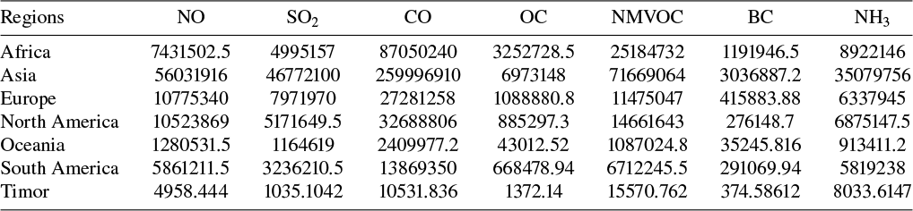
Our environment and human health are both badly affected by air pollution. In one year, approximately 7 million people died from outdoor and indoor air pollution as stated by the World Health Organisation (WHO). WHO have stated a range of polluted air that is safe for human breathing. However, at present, more than 99% of people breathe in air that is more polluted than this range. Air pollution is the fourth biggest curse for our atmosphere. As per the Global Air Report 2020, approximately 2.2 million have lost their lives due to indoor air pollution and approximately 4.5 million have lost their lives due to outdoor air pollution. India and China are the most polluted countries in the world as per data. Many other regions of the world are not far behind in the case of air pollution. Air pollution in different continents is a major talking point. Many substances are present in the air such as ammonia, black carbon, nonmethane volatile organic compounds, organic carbon, carbon monoxide, sulphur dioxide, nitrogen oxide, and so forth. A datasetFootnote 1 containing these substances in air in different continents is taken. Table 1 and Figure 8 present the actual dataset. Abbreviations used in Table 1 and Figure 8 are Nitrogen oxide (NO), sulphur dioxide (SO
 $_2$
), carbon monoxide (CO), organic carbon (OC), nonmethane volatile organic compounds (NMVOC), ammonia (NH
 $_3$
) and black carbon (BC).
Dataset for air pollution for the year 2022.

 $^*$
Data in this table is in metric tonnes.
Dataset for air pollution.

We use the proposed algorithm to create clusters for the given data set. For this, take into consideration the following cluster analysis issue.
Consider a cluster analysis issue containing a set of seven alternatives:
 $B_1, B_2, B_3, B_4, B_5, B_6, B_7$
used for Africa, Asia, Europe, North America, Oceania, South America, Timor, respectively. Let us consider a set of criteria:
 $C_1, C_2, C_3, C_4, C_5, C_6, C_7$
used for NO, SO
 $_2$
, CO, OC, NMVOC, BC, NH
 $_3$
, respectively. The alternatives and criteria are shown in Figure 9.
Alternatives and criteria.

Let us consider the set of criteria weights
 $A = \{a_1, a_2, \ldots , a_7\}$
, where
 $\sum _{\tau =1}^7 a_{\tau } =1$
and
 $0 \leq a_{\tau } \leq 1$
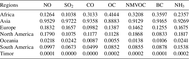
. The data in normalized form is shown in Table 2 by using the formula used by Singh and Kumar [Reference Singh and Kumar27].
Normalized data.

Now, the suggested algorithm is used to create clusters from these data. The steps in the suggested algorithm are as follows.
-
Step 1. Collect the data and convert it in the
$\mathbf {\mathcal {B}^{\mathcal {F}}}$
-framework. First of all, take the data from Table 2. These data are not in the
$\mathcal {B}^{\mathcal {F}}$
-framework. To convert these data in the
$\mathcal {B}^{\mathcal {F}}$
-framework, we make use of (5.1). The
$\mathcal {B}^{\mathcal {F}}$
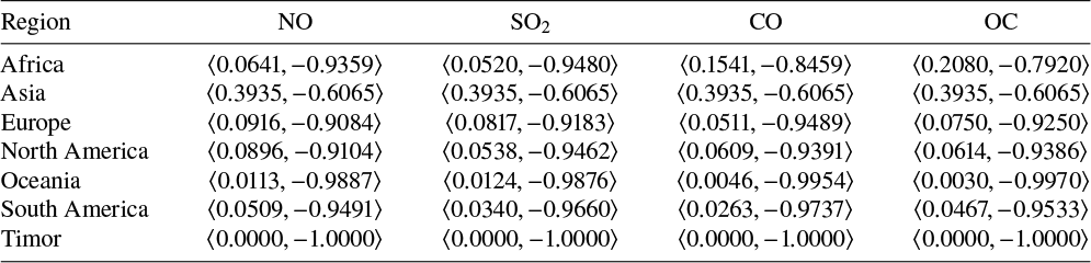
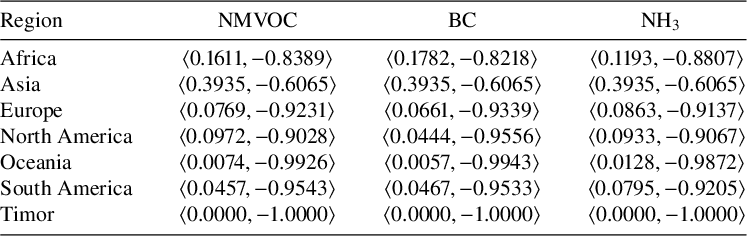
-matrix L is shown by Tables 3 and 4.Table 3Dataset for air pollution in
$\mathcal {B}^{\mathcal {F}}$
-framework for criteria
$C_1$
,
$C_2$
,
$C_3$
and
$C_4$
.Table 4Dataset for air pollution in
$\mathcal {B}^{\mathcal {F}}$
-framework for criteria
$C_5$
,
$C_6$
and
$C_7$
. -
Step 2. Construction of the accuracy matrix. With the help of Definition 5.1, an accuracy matrix D is constructed and its value is shown in the following. Matrix D is symmetrical and every element represents the accuracy between two alternatives,
$$ \begin{align*} D = \begin{pmatrix} 1 &0.5616 &0.6703 &0.6722 &0.7033 &0.6839 &0.7074 \\ 0.1822 &1 &0.2142 &0.2166 &0.2540 &0.2308 &0.2590 \\ 0.7726 &0.6958 &1 &0.7983 &0.8277 &0.8093 &0.8317 \\ 0.7817 &0.7054 &0.8055 &1 &0.8367 &0.8184 &0.8407 \\ 0.9266 &0.8566 &0.9487 &0.9505 &1 &0.9608 &0.9816 \\ 0.8371 &0.7634 &0.8603 &0.8621 &0.8907 &1 &0.8946 \\ 0.9454 &0.8763 &0.9674 &0.9692 &0.9963 &0.9794 &1 \\ \end{pmatrix}. \end{align*} $$
-
Step 3. Construction of the equivalent accuracy matrix. Apply the successive compositions, that is,
$D \rightarrow D^2 \rightarrow D^4 \rightarrow \cdots \rightarrow D^{2^z} \rightarrow \cdots $
for an accuracy matrix
$D = \{d_{{\omega }{\tau }}\}_{W \times W}$
. The powers of D are shown as follows:
$$ \begin{align*} \begin{aligned} D^2 & = D\ o\ D \\ &= \begin{pmatrix} 1.0000 & 0.7074 & 0.7074 & 0.7074 & 0.7074 & 0.7074 & 0.7074 \\ 0.2590 & 1.0000 & 0.2590 & 0.2590 & 0.2590 & 0.2590 & 0.2590 \\ 0.8317 & 0.8317 & 1.0000 & 0.8317 & 0.8317 & 0.8317 & 0.8317 \\ 0.8407 & 0.8407 & 0.8407 & 1.0000 & 0.8407 & 0.8407 & 0.8407 \\ 0.9454 & 0.8763 & 0.9674 & 0.9692 & 1.0000 & 0.9794 & 0.9816 \\ 0.8946 & 0.8763 & 0.8946 & 0.8946 & 0.8946 & 1.0000 & 0.8946 \\ 0.9454 & 0.8763 & 0.9674 & 0.9692 & 0.9963 & 0.9794 & 1.0000 \\ \end{pmatrix} \end{aligned}, \end{align*} $$
After successive compositions, we have
$$ \begin{align*} \begin{aligned} D^4 & = D^2\ o\ D^2 \\& = \begin{pmatrix} 1.0000 & 0.7074 & 0.7074 & 0.7074 & 0.7074 & 0.7074 & 0.7074 \\ 0.2590 & 1.0000 & 0.2590 & 0.2590 & 0.2590 & 0.2590 & 0.2590 \\ 0.8317 & 0.8317 & 1.0000 & 0.8317 & 0.8317 & 0.8317 & 0.8317 \\ 0.8407 & 0.8407 & 0.8407 & 1.0000 & 0.8407 & 0.8407 & 0.8407 \\ 0.9454 & 0.8763 & 0.9674 & 0.9692 & 1.0000 & 0.9794 & 0.9816 \\ 0.8946 & 0.8763 & 0.8946 & 0.8946 & 0.8946 & 1.0000 & 0.8946 \\ 0.9454 & 0.8763 & 0.9674 & 0.9692 & 0.9963 & 0.9794 & 1.0000 \\ \end{pmatrix} \end{aligned}. \end{align*} $$
$D^{2} = D^{4}$
. Thus, the resultant matrix
$D^{2}$
is the equivalent accuracy matrix.
-
Step 4. Find the values of confidence levels and make clusters from different
$\boldsymbol {\Psi }$
-cutting matrices. For different values of
$\Psi \in [0, 1]$
, generate the
$\Psi $
-cutting matrix
$M_{\Psi }$
by using Definition 5.5. Different values of
$\Psi $
in the given example are
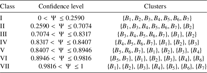
$\{0.2590, 0.7074, 0.8317, 0.8407, 0.8946, 0.9816, 1\}$
. For these values of
$\Psi $
, different
$\Psi $
-cutting matrices are formed. Two given alternatives
$B_\omega $
and
$B_\tau $
are from the same cluster if the
${\omega }$
th column or row is equal to the
${\tau }$
th column or row in these
$\Psi $
-cutting matrices. In the same way, we may group all the other alternatives to form various clusters. Table 5 shows different clusters.Table 5Cluster analysis by using proposed accuracy measure.
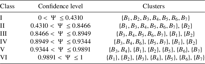
Table 6Cluster analysis by using a proposed similarity measure.


Table 5 examined that the suggested accuracy measure may effectively address the clustering issues. With the new approach, we get clusters. However, we can also use the proposed similarity measure in the above algorithm, then we get the output in Table 6. With the similarity measure approach, we get clusters. Hence, the new approach offers high clustering accuracy consequently.
5.2 Medical diagnoses
The process of identifying a problem from the symptoms of an individual and indications is known as a medical diagnosis. Many researchers have worked on this approach and have had good results using distance, correlation and similarity measures. Instead of using the provided measures, we use the proposed accuracy measure. Consider two examples given as follows.
Example 5.6. Consider a collection U of eight patients, a collection V of symptoms and a collection W of diagnosis, where
 $$ \begin{align*} \begin{aligned} U &= \{B_{\omega}\}_{\omega = 1}^{8}, \\[6pt] V &= \begin{Bmatrix} \text{Weakness or Numbness, Swelling, Skin problem, Cognitive changes,} \\ \text{Appetite problems, Nausea, Dyspnea, Fever, Pain, Fatigue} \end{Bmatrix}, \\[6pt] W &= \begin{Bmatrix} \text{Genetic disorders, Endocrine disorders, Gastrointestinal disorders,} \\ \text{Cancer, Autoimmune disorders, Mental Health disorders,} \\ \text{Neurological disorders, Cardiovascular diseases, Chronic diseases,} \\ \text{Infectious diseases}\end{Bmatrix}. \end{aligned} \end{align*} $$
The definitions of the symptoms of the patients are shown in Table 7 and the definitions of the symptoms of the diagnosis are shown in Table 8.
The definitions of the symptoms of the patients.

The definitions of the symptoms of the diagnosis.

The relation
 $U \rightarrow V \rightarrow W$
is used to represent the
 $\mathcal {B}^{\mathcal {F}}$
-numbers in Tables 9, 10, 11 and 12.
Patient’s symptoms (1–5).

Patient’s symptoms (6–10).

Diagnosis’s symptoms (1–5).

Diagnosis’s symptoms (6–10).

To develop a trustworthy diagnosis, we assessed the accuracy of patients and diagnoses about symptoms. We follow this procedure for every diagnosis. If the accuracy measure is high, the patient has that specific disease. Table 13 shows the accuracy between patients and diagnoses.
Symptoms of the diagnosis by using proposed accuracy measure.

According to Table 13, patients
 $B_1$
,
 $B_2$
and
 $B_7$
have Autoimmune disorders, patient
 $B_3$
has Endocrine disorders, patient
 $B_4$
has Genetic disorders, patient
 $B_5$
has Neurological disorders, patient
 $B_6$
has Cardiovascular diseases and patient
 $B_8$
has Cancer.
Example 5.7. Consider a collection U of five patients, a collection V of symptoms and a collection W of diagnosis, where
 $$ \begin{align*} \begin{aligned} U &= \{B_{\omega}\}_{\omega = 1}^{5}, \\ V &= \begin{Bmatrix} \text{Irritation, Chest pain, Running nose, Cough, Sore throat,} \\ \text{Stomach pain, Headache, Fever}\end{Bmatrix}, \\ W &= \{\text{Malaria, Heart problem, Stomach problem, Viral fever, Typhoid} \}. \end{aligned} \end{align*} $$
The relation
 $U \rightarrow V \rightarrow W$
is used to represent the
 $\mathcal {B}^{\mathcal {F}}$
-numbers in the Tables 14 and 15.
Patient’s symptoms.

Diagnosis’s symptoms.

To develop a trustworthy diagnosis, we assessed the accuracy of patients and diagnoses about symptoms. We follow this procedure for every diagnosis. If the accuracy measure is high, the patient has that specific disease. Table 16 shows the accuracy between patients and diagnoses.
Symptoms of the diagnosis.

According to Table 16, patients
 $B_1$
has Viral fever, patients
 $B_2$
and
 $B_5$
have Malaria, patient
 $B_3$
has Heart problem, and patient
 $B_4$
has Typhoid. Hence, the proposed accuracy measure successfully solves the problems related to medical diagnosis.
5.3 Pattern detection
The process of categorizing a random pattern into certain recognized patterns is known as pattern detection. Many academics have concentrated on the pattern detection approach and have employed similarity, correlation and distance measurements to get effective results. We use the derived measures to solve pattern detection issues. For this, take two examples as follows.
Example 5.8. Let
 $K = \{0, 9, 1, 8, 2, 7, 3, 6, 4, 5\}$
be a finite set containing ten elements. Take the following patterns in the form of
 $\mathcal {B}^{\mathcal {F}}$
-sets as follows:
 $$ \begin{align*} B_1 = \begin{Bmatrix} \langle 0, (0.44, -0.45) \rangle, \ \langle 9, (0.74, -0.78) \rangle, \ \langle 1, (0.22, -0.52) \rangle, \\ \langle 8, (0.56, -0.36) \rangle, \ \langle 2, (0.36, -0.98) \rangle, \ \langle 7, (0.45, -0.25) \rangle, \\ \langle 3, (0.54, -0.01) \rangle, \ \langle 6, (0.69, -0.26) \rangle, \ \langle 4, (0.78, -0.45) \rangle, \\ \langle 5, (0.42, -0.78) \rangle \end{Bmatrix}, \end{align*} $$
 $$ \begin{align*} B_2 = \begin{Bmatrix} \langle 0, (0.45, -0.45) \rangle, \ \langle 9, (0.58, -0.78) \rangle, \ \langle 1, (0.20, -0.56) \rangle, \\ \langle 8, (0.32, -0.96) \rangle, \ \langle 2, (0.56, -0.82) \rangle, \ \langle 7, (0.56, -0.01) \rangle, \\ \langle 3, (0.87, -0.36) \rangle, \ \langle 6, (0.45, -0.87) \rangle, \ \langle 4, (0.42, -0.45) \rangle, \\ \langle 5, (0.10, -0.15) \rangle \end{Bmatrix}, \end{align*} $$
 $$ \begin{align*} B_3 = \begin{Bmatrix} \langle 0, (0.56, -0.54) \rangle, \ \langle 9, (0.87, -0.69) \rangle, \ \langle 1, (0.10, -0.87) \rangle, \\ \langle 8, (0.29, -0.75) \rangle, \ \langle 2, (0.92, -0.35) \rangle, \ \langle 7, (0.45, -0.60) \rangle, \\ \langle 3, (0.73, -0.20) \rangle, \ \langle 6, (0.38, -0.87) \rangle, \ \langle 4, (0.87, -0.52) \rangle, \\ \langle 5, (0.45, -0.36) \rangle \end{Bmatrix}, \end{align*} $$
 $$ \begin{align*} B_4 = \begin{Bmatrix} \langle 0, (0.56, -0.03) \rangle, \ \langle 9, (0.87, -0.68) \rangle, \ \langle 1, (0.20, -0.76) \rangle, \\ \langle 8, (0.35, -0.34) \rangle, \ \langle 2, (0.69, -0.06) \rangle, \ \langle 7, (0.84, -0.20) \rangle, \\ \langle 3, (0.56, -0.34) \rangle, \ \langle 6, (0.54, -0.56) \rangle, \ \langle 4, (0.20, -0.54) \rangle, \\ \langle 5, (0.35, -0.08) \rangle \end{Bmatrix}, \end{align*} $$
 $$ \begin{align*} B_5 = \begin{Bmatrix} \langle 0, (0.56, -0.20) \rangle, \ \langle 9, (0.31, -0.36) \rangle, \ \langle 1, (0.78, -0.87) \rangle, \\ \langle 8, (0.96, -0.92) \rangle, \ \langle 2, (0.54, -0.57) \rangle, \ \langle 7, (0.52, -0.63) \rangle, \\ \langle 3, (0.10, -0.49) \rangle, \ \langle 6, (0.65, -0.28) \rangle, \ \langle 4, (0.85, -0.62) \rangle, \\ \langle 5, (0.65, -0.10) \rangle \end{Bmatrix}, \end{align*} $$
 $$ \begin{align*} B_6 = \begin{Bmatrix} \langle 0, (0.69, -0.54) \rangle, \ \langle 9, (0.89, -0.63) \rangle, \ \langle 1, (0.65, -0.25) \rangle, \\ \langle 8, (0.35, -0.78) \rangle, \ \langle 3, (0.38, -0.96) \rangle, \ \langle 7, (0.64, -0.35) \rangle, \\ \langle 4, (0.02, -0.64) \rangle, \ \langle 6, (0.65, -0.10) \rangle, \ \langle 4, (0.45, -0.36) \rangle, \\ \langle 5, (0.65, -0.54) \rangle \end{Bmatrix}, \end{align*} $$
 $$ \begin{align*} B_7 = \begin{Bmatrix} \langle 0, (0.45, -0.25) \rangle, \ \langle 9, (0.63, -0.63) \rangle, \ \langle 1, (0.57, -0.30) \rangle, \\ \langle 8, (0.89, -0.12) \rangle, \ \langle 2, (0.65, -0.45) \rangle, \ \langle 7, (0.30, -0.89) \rangle, \\ \langle 3, (0.39, -0.65) \rangle, \ \langle 6, (0.67, -0.45) \rangle, \ \langle 4, (0.85, -0.22) \rangle, \\ \langle 5, (0.65, -0.15) \rangle \end{Bmatrix}, \end{align*} $$
 $$ \begin{align*} B_8 = \begin{Bmatrix} \langle 0, (0.20, -0.45) \rangle, \ \langle 9, (0.32, -0.63) \rangle, \ \langle 1, (0.36, -0.56) \rangle, \\ \langle 8, (0.89, -0.87) \rangle, \ \langle 2, (0.72, -0.10) \rangle, \ \langle 7, (0.83, -0.24) \rangle, \\ \langle 3, (0.55, -0.56) \rangle, \ \langle 6, (0.24, -0.52) \rangle, \ \langle 4, (0.55, -0.45) \rangle, \\ \langle 5, (0.23, -0.56) \rangle \end{Bmatrix}, \end{align*} $$
 $$ \begin{align*} B_9 = \begin{Bmatrix} \langle 0, (0.26, -0.56) \rangle, \ \langle 9, (0.35, -0.96) \rangle, \ \langle 1, (0.40, -0.13) \rangle, \\ \langle 8, (0.50, -0.54) \rangle, \ \langle 2, (0.65, -0.56) \rangle, \ \langle 7, (0.45, -0.50) \rangle, \\ \langle 3, (0.52, -0.67) \rangle, \ \langle 6, (0.20, -0.98) \rangle, \ \langle 4, (0.36, -0.85) \rangle, \\ \langle 5, (0.69, -0.20) \rangle \end{Bmatrix}, \end{align*} $$
 $$ \begin{align*} B_{10} = \begin{Bmatrix} \langle 0, (0.63, -0.69) \rangle, \ \langle 9, (0.21, -0.63) \rangle, \ \langle 1, (0.56, -0.32) \rangle, \\ \langle 8, (0.30, -0.45) \rangle, \ \langle 2, (0.36, -0.65) \rangle, \ \langle 7, (0.94, -0.58) \rangle, \\ \langle 3, (0.85, -0.99) \rangle, \ \langle 6, (0.66, -0.95) \rangle, \ \langle 4, (0.84, -0.64) \rangle, \\ \langle 5, (0.09, -0.23) \rangle \end{Bmatrix}. \end{align*} $$
Let an unknown pattern in the form of the
 $\mathcal {B}^{\mathcal {F}}$
-set be given by
 $$ \begin{align*} B = \begin{Bmatrix} \langle 0, (0.65, -0.56) \rangle, \ \langle 9, (0.63, -0.89) \rangle, \ \langle 1, (0.23, -0.78) \rangle, \\ \langle 8, (0.78, -0.54) \rangle, \ \langle 2, (0.95, -0.22) \rangle, \ \langle 7, (0.12, -0.65) \rangle, \\ \langle 3, (0.65, -0.45) \rangle, \ \langle 6, (0.45, -0.23) \rangle, \ \langle 4, (0.56, -0.25) \rangle, \\ \langle 5, (0.21, -0.75) \rangle \end{Bmatrix}. \end{align*} $$
Using the derived measures, we identify which pattern fits within B the best. Using the derived measures and some previously known measures yields the results in Table 17.
Pattern detection using proposed measures and previously known measures.

From Table 17, the pattern B fits best in the pattern
 $B_3$
by using the derived measures. Also, by using the distance measure
 $NH_d$
in (2.1) and distance measure
 $NH_e$
in (2.2), the pattern B fits best in the pattern
 $B_3$
.
Example 5.9. Let
 $K \{5, 10, 15, 20, 25, 30, 35, 40, 45, 50, 55, 60, 65, 70, 75\}$
be a finite set containing fifteen elements. Take the following patterns in the form of
 $\mathcal {B}^{\mathcal {F}}$
-sets:
 $$ \begin{align*} B_1 = \begin{Bmatrix} \langle 5, (0.03, -0.45) \rangle, \ \langle 10, (0.87, -0.63) \rangle, \ \langle 15, (0.45, -0.21) \rangle, \\ \langle 20, (0.96, -0.02) \rangle, \ \langle 25, (0.30, -0.89) \rangle, \ \langle 30, (0.57, -0.78) \rangle, \\ \langle 35, (0.89, -0.54) \rangle, \ \langle 40, (0.50, -0.62) \rangle, \ \langle 45, (0.36, -0.36) \rangle, \\ \langle 50, (0.54, -0.54) \rangle, \ \langle 55, (0.12, -0.87) \rangle, \ \langle 60, (0.01, -0.80) \rangle, \\ \langle 65, (0.23, -0.25) \rangle, \ \langle 70, (0.56, -0.60) \rangle, \ \langle 75, (0.58, -0.89) \rangle \end{Bmatrix}, \end{align*} $$
 $$ \begin{align*} B_2 = \begin{Bmatrix} \langle 5, (0.56, -0.15) \rangle, \ \langle 10, (0.45, -0.96) \rangle, \ \langle 15, (0.20, -0.35) \rangle, \\ \langle 20, (0.36, -0.78) \rangle, \ \langle 25, (0.56, -0.95) \rangle, \ \langle 30, (0.30, -0.32) \rangle, \\ \langle 35, (0.29, -0.06) \rangle, \ \langle 40, (0.78, -0.98) \rangle, \ \langle 45, (0.52, -0.70) \rangle, \\ \langle 50, (0.36, -0.29) \rangle, \ \langle 55, (0.58, -0.52) \rangle, \ \langle 60, (0.19, -0.01) \rangle, \\ \langle 65, (0.20, -0.23) \rangle, \ \langle 70, (0.15, -0.56) \rangle, \ \langle 75, (0.05, -0.58) \rangle \end{Bmatrix}, \end{align*} $$
 $$ \begin{align*} B_3 = \begin{Bmatrix} \langle 5, (0.21, -0.56) \rangle, \ \langle 10, (0.34, -0.82) \rangle, \ \langle 15, (0.65, -0.03) \rangle, \\ \langle 20, (0.42, -0.68) \rangle, \ \langle 25, (0.03, -0.56) \rangle, \ \langle 30, (0.22, -0.45) \rangle, \\ \langle 35, (0.60, -0.21) \rangle, \ \langle 40, (0.58, -0.65) \rangle, \ \langle 45, (0.30, -0.78) \rangle, \\ \langle 50, (0.15, -0.52) \rangle, \ \langle 55, (0.45, -0.02) \rangle, \ \langle 60, (0.21, -0.15) \rangle, \\ \langle 65, (0.65, -0.45) \rangle, \ \langle 70, (0.20, -0.56) \rangle, \ \langle 75, (0.20, -0.62) \rangle \end{Bmatrix}, \end{align*} $$
 $$ \begin{align*} B_4 = \begin{Bmatrix} \langle 5, (0.56, -0.90) \rangle, \ \langle 10, (0.59, -0.36) \rangle, \ \langle 15, (0.57, -0.98) \rangle, \\ \langle 20, (0.56, -0.97) \rangle, \ \langle 25, (0.69, -0.54) \rangle, \ \langle 30, (0.54, -0.96) \rangle, \\ \langle 35, (0.82, -0.54) \rangle, \ \langle 40, (0.92, -0.58) \rangle, \ \langle 45, (0.91, -0.78) \rangle, \\ \langle 50, (0.36, -0.52) \rangle, \ \langle 55, (0.54, -0.72) \rangle, \ \langle 60, (0.58, -0.54) \rangle, \\ \langle 65, (0.95, -0.65) \rangle, \ \langle 70, (0.80, -0.85) \rangle, \ \langle 75, (0.92, -0.78) \rangle \end{Bmatrix}, \end{align*} $$
 $$ \begin{align*} B_5 = \begin{Bmatrix} \langle 5, (0.21, -0.30) \rangle, \ \langle 10, (0.53, -0.56) \rangle, \ \langle 15, (0.25, -0.12) \rangle, \\ \langle 20, (0.65, -0.00) \rangle, \ \langle 25, (0.45, -0.10) \rangle, \ \langle 30, (0.21, -0.59) \rangle, \\ \langle 35, (0.50, -0.54) \rangle, \ \langle 40, (0.56, -0.85) \rangle, \ \langle 45, (0.54, -0.30) \rangle, \\ \langle 50, (0.78, -0.23) \rangle, \ \langle 55, (0.52, -0.65) \rangle, \ \langle 60, (0.53, -0.02) \rangle, \\ \langle 65, (0.25, -0.12) \rangle, \ \langle 70, (0.51, -0.78) \rangle, \ \langle 75, (0.56, -0.51) \rangle \end{Bmatrix}, \end{align*} $$
 $$ \begin{align*} B_6 = \begin{Bmatrix} \langle 5, (0.25, -0.52) \rangle, \ \langle 10, (0.30, -0.56) \rangle, \ \langle 15, (0.50, -0.84) \rangle, \\ \langle 20, (0.04, -0.65) \rangle, \ \langle 25, (0.54, -0.32) \rangle, \ \langle 30, (0.50, -0.02) \rangle, \\ \langle 35, (0.27, -0.54) \rangle, \ \langle 40, (0.79, -0.87) \rangle, \ \langle 45, (0.65, -0.49) \rangle, \\ \langle 50, (0.65, -0.65) \rangle, \ \langle 55, (0.02, -0.20) \rangle, \ \langle 60, (0.33, -0.32) \rangle, \\ \langle 65, (0.56, -0.45) \rangle, \ \langle 70, (0.98, -0.45) \rangle, \ \langle 75, (0.65, -0.85) \rangle \end{Bmatrix}. \end{align*} $$
Let an unknown pattern in the form of the
 $\mathcal {B}^{\mathcal {F}}$
-set be given by
 $$ \begin{align*} B = \begin{Bmatrix} \langle 5, (0.56, -0.20) \rangle, \ \langle 10, (0.58, -0.36) \rangle, \ \langle 15, (0.95, -0.90) \rangle, \\ \langle 20, (0.63, -0.87) \rangle, \ \langle 25, (0.45, -0.45) \rangle, \ \langle 30, (0.78, -0.65) \rangle, \\ \langle 35, (0.52, -0.20) \rangle, \ \langle 40, (0.03, -0.30) \rangle, \ \langle 45, (0.65, -0.56) \rangle, \\ \langle 50, (0.65, -0.87) \rangle, \ \langle 55, (0.78, -0.89) \rangle, \ \langle 60, (0.96, -0.66) \rangle, \\ \langle 65, (0.39, -0.20) \rangle, \ \langle 70, (0.90, -0.32) \rangle, \ \langle 75, (0.54, -0.15) \rangle \end{Bmatrix}. \end{align*} $$
Using the derived measures, we identify which pattern fits within B the best. Using the derived measures and some previously known measures yields the results in Table 18.
Pattern detection using proposed measures and previously known measures.

From Table 18, the pattern B fits best in the pattern
 $B_4$
by using the derived measures. Also, by using the distance measure
 $NH_d$
in (2.1) and distance measure
 $NH_e$
in (2.2), the pattern B fits best in the pattern
 $B_4$
. Both these examples of pattern detection imply the efficacy of the proposed measures.
6 Conclusion
The
 $\phi $
-norm entropy concept is used to propose a
 $\mathcal {B}^{\mathcal {F}}$
knowledge-measure in this manuscript. The proposed measure’s basic properties are investigated. By using numerical illustrations, the utility of the measure is demonstrated. The proposed measure is used to create and validate an accuracy measure. Some properties are discussed in the
 $\mathcal {B}^{\mathcal {F}}$
-framework. Additionally, similarity and dissimilarity measures in the
 $\mathcal {B}^{\mathcal {F}}$
-framework are derived from the proposed measure and validated. Using the proposed measures, the issues with pattern detection, cluster analysis and medical diagnosis are resolved. In the current work, a novel
 $\mathcal {B}^{\mathcal {F}}$
-clustering approach is developed employing the proposed accuracy measure. The official website provides real data on air pollution in different regions in the year 2022. The proposed approach is then used on this data to create clusters. Additionally, two examples of pattern detection as well as medical diagnosis issues are addressed by using the derived measures. In the future, the intended study may be expanded upon in several ways.
-
(1) The proposed
$\mathcal {B}^{\mathcal {F}}$
knowledge-measure may be extended to the Bipolar complex fuzzy set,
$\mathcal {B}^{\mathcal {F}}$
-Soft set, n-Polar fuzzy sets and so on. -
(2) The resulting
$\mathcal {B}^{\mathcal {F}}$
-accuracy measure may also be used to create a decision-making approach that we can use to resolve decision-making problems in the
$\mathcal {B}^{\mathcal {F}}$
-framework. -
(3) In the future, we may use the derived measures to the issue of green supplier selection and image processing.


We may also use the proposed methods to solve several real-world problems. Furthermore, we will make a concerted effort in the next years to rectify any deficiencies in the proposed study. Thus, the proposed approach has several practical applications.