





1. Introduction
The spectral gap
 $\lambda_1(X)$
of a closed orientable hyperbolic surface X is the minimal non-zero eigenvalue of its Laplacian. A natural question, which fits into a larger context of the study of the bass note spectra of locally uniform geometries [Reference SarnakSar23], is which numbers appear as spectral gaps of hyperbolic surfaces. It can be derived in various ways from various combinations of [Reference HuberHub74, Reference ChengChe75, Reference BuserBus77, Reference GageGag80, Reference JenniJen81, Reference BavardBav96, Reference Strohmaier and UskiSU13, Reference BonifacioBon22, Reference Fortier Bourque and PetriFP23, Reference Kravchuk, Mazáč and PalKMP24] that the bass note spectrum of the set of closed orientable hyperbolic surfaces satisfies
 $$\mathrm{Bass}(\mathbf{hyp}_2^c) := \{ \lambda_1(X) : X \text{ a closed orientable hyperbolic surface}\} = (0,\Lambda_2],$$
where
 $\Lambda_2 = \max\{ \lambda_1(X) : X \text{ a closed hyperbolic surface of genus }2\}$
. The latter conjecturally equals the spectral gap of the Bolza surface (see § 2.1 for a description).
If we restrict to arithmetic surfaces, the set of spectral gaps we obtain becomes countable. Recently, Magee [Reference MageeMag24a] proved that the spectral gaps, defined as the infimum of the non-zero spectrum in this setting, of non-compact arithmetic surfaces form a dense set in
 $[0,\frac{1}{4}]$
. He also asked whether the same is true for closed arithmetic surfaces. The goal of this paper is to answer this question in the affirmative.
Theorem 1.
The set
 $\{\lambda_1(X) : X\text{ a closed arithmetic surface} \}\cap [0,\frac{1}{4}]$
is dense in
 $[0,\frac{1}{4}]$
.
In fact, we show that, as in the non-compact case, it suffices to consider only finite-index torsion-free subgroups of a single uniform arithmetic group. In our case this is the (2,3,8)-triangle group.
Similarly, the same method can be used to prove that if
 $X=\Gamma\backslash\mathbb{H}^2$
is a closed orientable surface then
 $$ \{\lambda_1(\Gamma'\backslash\mathbb{H}^2) : \Gamma'\lt\Gamma,\; [\Gamma:\Gamma'] \lt \infty \}\cap [0,\Lambda]$$
is dense in
 $[0,\Lambda]$
, where
 $\Lambda = \min\{ \lambda_1(\Gamma'\backslash\mathbb{H}^2) : \Gamma'\lt\Gamma,\; [\Gamma:\Gamma']=2\}$
.
Finally, we also obtain a different proof of [Reference Louder, Magee and HideLMH25, Theorem 1.8], the fact that there exists a sequence of finite-sheeted covers
 $Y_n\to X$
of a fixed closed orientable arithmetic hyperbolic surface X, whose genera tend to infinity and whose spectral gap tends to
 $\frac{1}{4}$
.
1.1 Strategy of proof
Like Magee’s proof in the non-uniform case, we build our arithmetic surfaces as covers of degree 2 of a certain type of random covers of a fixed base surface. In our case, this base surface is the Bolza surface
 $X_B$
. As such, the overarching strategy of our proof is similar to that of Magee. However, several of the key ingredients of his proof are not present in our setting, so in what follows we will describe the similarities and differences.
The first thing that makes our case different is that the fundamental group
 $\Gamma_B=\pi_1(X_B)$
of the
 $X_B$
is not free, which makes random finite-degree covers harder to control (see [Reference Magee and PuderMP23, Reference Magee, Naud and PuderMNP22] for the geometry of uniform random covers of a closed hyperbolic surface). We remedy this by considering random covers
 $Y^{(n)}\to X_B$
of degree n whose monodromy factors through an epimorphism from our surface group
 $\Gamma_B\to F_2$
to a free group
 $F_2$
on two generators. This allows us to use the results of Bordenave and Collins [Reference Bordenave and CollinsBC19] on strong convergence of permutation representations combined with results by Hide and Magee [Reference Louder, Magee and HideLMH25, Appendix] on the convergence of the spectral gaps of the associated covers. In [Reference Louder, Magee and HideLMH25], Louder and Magee also did this. However, we need more control over the geometry of the associated cover, so we use a different argument.
We need to control the following things.
-
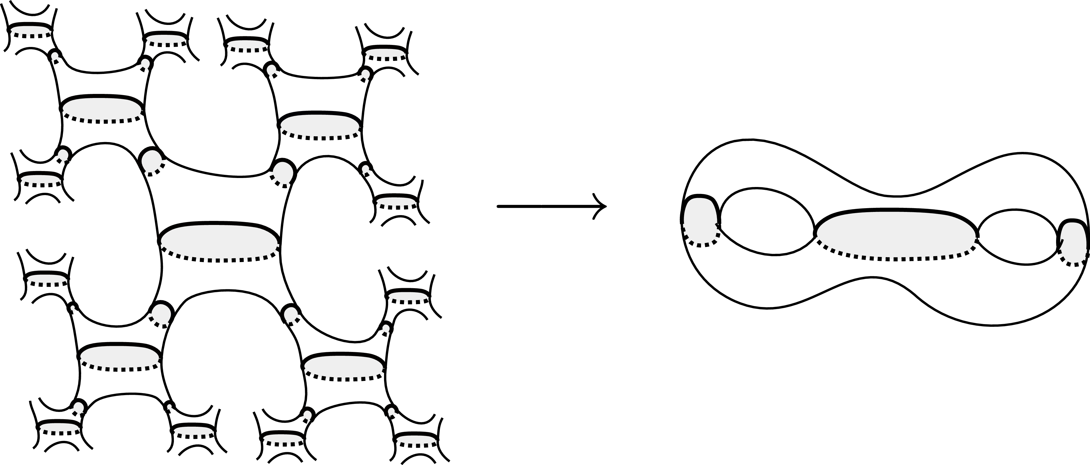
(1) In order to obtain near-optimal spectral gaps, we need to understand the spectral gap of the cover of the Bolza surface associated to the map
 $\Gamma_B\to F_2$
(see Figure 1). We tackle this using Cheeger’s inequality. Using Mirzakhani’s result on random pants decompositions of hyperbolic surfaces [Reference MirzakhaniMir16] combined with some further geometric arguments, we show that by varying the map to the free group (see § 4 and Proposition 6.1) we can obtain a spectral gap as close to
$\frac{1}{4}$
as we like.Figure 1.
A tree cover of a surface of genus 2.
-
(2) To reach intermediate spectral gaps, our aim is to use the covers of degree 2 of our random cover
$Y^{(n)}\to X_B$
. To make this work, we need there to be at least one cover among these degree 2 covers that has a large spectral gap. We obtain such a cover by restricting a non-constant homomorphism
$\Gamma_B\to F_2\to\mathbb{Z}/2\mathbb{Z}$
to the fundamental group of
$Y^{(n)}$
, seen as a subgroup of
$\Gamma_B$
. The fact that this indeed yields two-sheeted covers of
$Y^{(n)}$
with large spectral gaps relies on a strong convergence argument combined with the fact that all connected two-sheeted covers
$\widehat{Y}\to X_B$
satisfy
$\lambda_1(\widehat{Y})\gt\frac{1}{4}$
. The latter fact we prove (in § 3) using the linear programming methods developed in [Reference Fortier Bourque and PetriFP23, Reference Fortier Bourque, Gruda-Mediavilla, Petri and PineaultFGP+23]. -
(3) Like Magee, we then need to show that, when n is large enough, ‘small’ modifications of the degree 2 covers of
$Y^{(n)}$
do not influence the spectral gap too much. These modifications consist of changing the cover along the lifts of a simple closed curve in
$Y^{(n)}$
and will be called switches (see § 6.5). In Magee’s paper, logarithmic tangle-freeness is used to prove that similar moves do not influence the spectral gap too much. Unfortunately, our covers are, by construction, much less tangle-free: the infinite cover associated to the map
$\Gamma_B\to F_2$
contains many short curves. As a result, the injectivity radius of
$Y^{(n)}$
is uniformly bounded.


We will show, however, again relying on Mirzakhani’s results on random pants decompositions and also using Nica’s work on cycles of random permutations coming from word maps [Reference NicaNic94], that we can find maps
 $\Gamma_B\to F_2$
such that, with positive probability, the curves in
 $Y^{(n)}$
along which we switch admit uniformly wide collars (see § 6.6). This suffices to make the argument, based on the
 $L^\infty$
-bounds on eigenfunctions by Gilmore et al. [Reference Gilmore, Le Masson, Sahlsten and ThomasGLS+21], work. This implies the density result because any two covers of degree 2 of
 $Y^{(n)}$
can be connected by a finite sequence of switches.
1.2 Further notes and references
The study of spectral gaps of hyperbolic surfaces has a long history, which we will not attempt to summarize here. We refer to [Reference BuserBus10, Reference BergeronBer16] for introductory texts. The shape of the bass note spectrum has been studied in the case of compact hyperbolic 2-orbifolds [Reference BonifacioBon22, Reference Kravchuk, Mazáč and PalKMP24], non-compact arithmetic surfaces [Reference MageeMag24a] and regular graphs [Reference Alon and WeiAW23, Reference Dong and McKenzieDM26]. In the case of orbifolds, Kravchuk, Mazac and Pal give a complete description of the set
 $$\{ \lambda_1(O) : O\text{ a compact orientable hyperbolic }2\text{-orbifold}\}.$$
This description is conjectural, but a large part of it is proven (see [Reference Kravchuk, Mazáč and PalKMP24, Conjecture 4.2]).
The case of arithmetic surfaces is very different. There are only finitely many arithmetic hyperbolic surfaces of any given area (up to isometry). As such, for any
 $\varepsilon\gt0$
, there can be at most finitely many closed arithmetric surfaces whose spectral gap exceeds
 $\frac{1}{4}+\varepsilon$
, using, for instance, the results in [Reference HuberHub74, Reference ChengChe75]. Hence, the theorem above can be stated as saying that the set of limit points of the set of spectral gaps of closed hyperbolic surfaces equals
 $[0,\frac{1}{4}]$
. There are, however, isolated points outside of this interval, corresponding, for instance, to the Bolza surface and the Klein quartic. Sarnak [Reference SarnakSar23] conjectured that there should be infinitely many such isolated points.
2. The model
In this section we formally describe our model of random surfaces, which is a variation of the models appearing in [Reference Budzinski, Curien and PetriBCP21, Reference Louder, Magee and HideLMH25, Reference MathienMat24].
2.1 The Bolza surface
The model we will describe samples a certain type of covers of a closed hyperbolic surface. The model makes sense for any closed base surface, but because of the application we have in mind, we will assume the base surface is the Bolza surface. We will use this subsection to describe some of its properties.
The quickest way to define the Bolza surface, which we denote by
 $X_B$
, is to say that it is a Riemann surface of genus 2 with 48 automorphisms. Indeed, it turns out that this is the maximal possible number of automorphisms of a Riemann surface of genus 2 and there is a unique such surface. More concretely,
 $X_B$
can be obtained by taking a regular octagon O with interior angles
 $\pi/4$
in the hyperbolic plane
 $\mathbb{H}^2$
and identifying opposite sides. We will also fix a Fuchsian group
 $\Gamma_B$
such that
 $X_B = \Gamma_B \backslash \mathbb{H}^2$
and we will, moreover, fix an identification of
 $\Gamma_B$
with
 $\pi_1(X_B)$
.
The surface
 $X_B$
is also a (2,3,8)-triangle surface. That is, its fundamental group is a normal subgroup (of index 48) in the orientable triangle group
 $$\Theta(2,3,8) = \langle x,y,z|\; x^2,\; y^3,\; z^8,\; xyz\rangle$$
whose generators act on
 $\mathbb{H}^2$
by the order 2, 3 and 8 rotations in the vertices of a hyperbolic triangle whose interior angles are
 $\pi/2$
,
 $\pi/3$
an
 $\pi/8$
, respectively. The quotient group is described explicitly as item T2.1 in [Reference ConderCon15]. Since the (2,3,8)-triangle group is arithmetic [Reference TakeuchiTak77] (see also [Reference Maclachlan and ReidMR03, § 13.3]),
 $X_B$
is arithmetic.
Very good numerical estimates of the spectral gap of
 $X_B$
have been obtained in [Reference Strohmaier and UskiSU13]. That is,
 $$\lambda_1(X_B) = 3.838887 \pm 10^{-6}.$$
The best known upper bound on the maximal spectral gap of a hyperbolic surface of genus 2 equals
 $3.8388976481$
[Reference BonifacioBon22, Reference Kravchuk, Mazáč and PalKMP24].
2.2 Handlebody attachments, maps to free groups and pants decompositions
A handlebody H is a 3-manifold that can be obtained by attaching 1-handles to a closed 3-ball. Alternatively, it can be seen as the closed regular neighbourhood of a finite graph in
 $\mathbb{R}^3$
. In particular, its fundamental group is a free group and its boundary is a closed orientable surface. The genus of this surface will be called the genus of H. This genus coincides with the rank of the fundamental group of H. The inclusion map
 $\iota:\partial H\hookrightarrow H$
induces an epimorphism
 $$\iota_*:\pi_1(\partial H) \longrightarrow F_g,$$
where g is the genus of H and
 $F_g$
denotes the free group of rank g. In fact, we obtain a large family of such maps, because we can precompose the inclusion by a homeomorphism
 $\phi:\partial H \to \partial H$
.
Any such homeomorphism yields an
 $F_g$
-cover
 $$T_\phi \to \partial H$$
corresponding to the subgroup
 $\ker((\iota\circ\phi)_*)$
. The surface
 $T_\phi$
is what is sometimes called a Cantor tree: a surface homeomorphic to
 $\mathbb{S}^2-C$
, where C is a Cantor set. As such, we will call the
 $F_g$
-covers constructed by the procedure above tree covers.
Finally, we observe that
 $\partial H$
admits a pants decomposition
 $\mathcal{P}$
consisting entirely of meridians: simple closed curves that bound disks in H (see Figure 1 for the case of genus 2). This means in particular that all the curves in
 $\mathcal{P}$
are homotopically trivial in H and thus that all the curves in the pants decomposition
 $\phi^{-1}(\mathcal{P})$
lie in
 $\ker((\iota\circ\phi)_*)$
. This in turn implies that
 $\phi^{-1}(\mathcal{P})$
lifts to a pants decomposition of
 $T_\phi$
(see Figure 1 again for a picture).
2.3 Random covers
We will now once and for all fix a handlebody attachment
 $\iota:X_B\hookrightarrow H$
of the Bolza surface
 $X_B$
and a pants decomposition
 $\mathcal{P}_0=(\alpha_1,\alpha_2,\alpha_3)$
of the
 $X_B$
that consists entirely of meridians.
Given an orientation-preserving homeomorphism
 $\phi:X_B\to X_B$
, we obtain, as in the previous section, a homomorphism
 $(\iota \circ \phi)_*:\Gamma_B \to F_2$
and a tree cover
 $T_\phi \to X_B$
. The pants decomposition of
 $T_\phi$
that we obtain by lifting
 $\phi^{-1}(\mathcal{P}_0)$
will be called the canonical pants decomposition of
 $T_\phi$
in what follows.
Now, given a homomorphism
 $\rho\in\textrm{Hom}(F_2,\mathfrak{S}_n)$
, where
 $\mathfrak{S}_n$
denotes the symmetric group on n letters, we obtain a subgroup
 $$H^{(n)} = \mathrm{Stab}_\rho(\{1\}) \lt F_2,$$
but also a homomorphism
 $$\rho\circ (\iota \circ\phi)_*:\Gamma_B \longrightarrow \mathfrak{S}_n,$$
and hence a subgroup
 $$\Lambda_{\phi,\rho} = \mathrm{Stab}_{\rho\circ (\iota \circ\phi)_*}(\{1\}) \lt \Gamma_B$$
of index at most n, and thus a cover
 $$Y_{\phi,\rho} \longrightarrow X_B$$
of degree at most n.
Our random surface
 $Y_\phi^{(n)}$
will be obtained by taking the permutation representation
 $\rho \in\textrm{Hom}(F_2,\mathfrak{S}_n)$
uniformly at random. It follows from results by Dixon [Reference DixonDix69] that, as
 $n\to\infty$
, the probability that the cover
 $Y_\phi^{(n)}$
is of degree exactly n tends to 1.
3. The bass notes of degree 2 covers of the Bolza surface
In this section we will explain how we prove, with the help of a computer, that all the degree 2 covers
 $Y\to X_B$
of the Bolza surface satisfy
 $\lambda_1(Y) \gt \frac{1}{4}$
. To do so, we will employ the linear programming methods from [Reference Fortier Bourque and PetriFP23, Reference Fortier Bourque, Gruda-Mediavilla, Petri and PineaultFGP+23].
In fact, just as in [Reference MageeMag24a], this can be proved by verifying the spectral gap of a single surface
 $Y_{17}$
obtained as the
 $\mathrm{H}_1(X_B,\mathbb{Z}/2\mathbb{Z})$
-cover of
 $X_B$
. Indeed, any homomorphism
 $\Gamma_B\to\mathbb{Z}/2\mathbb{Z}$
factors through
 $\mathrm{H}_1(X_B,\mathbb{Z}/2\mathbb{Z})$
and as such any degree 2 cover of
 $X_B$
is intermediate to the cover
 $Y_{17}\to X_B$
.
3.1 Identifying the cover
First of all, we need a description of
 $Y_{17}$
. Since
 $$| \mathrm{H}_1(X_B,\mathbb{Z}/2\mathbb{Z}) |=16,$$
the genus of
 $Y_{17}$
equals 17 (whence the notation). Moreover, by construction, the fundamental group of
 $Y_{17}$
is a characteristicFootnote
1
subgroup of
 $\Gamma_B$
. This implies that it is a normal subgroup of the (2,3,8)-triangle group
 $\Theta(2,3,8)$
. In other words,
 $Y_{17}$
is a (2,3,8)-triangle surface of genus 17. It turns out there is only one such surface, which appears as item T17.2 in Conder’s list [Reference ConderCon15]. In particular,
 $Y_{17}$
corresponds to the quotient
 $$G= \langle x,y,z|\; x^2,\; y^3,\; z^8,\; xyz,\; z^2 y x z^2 y x z y^{-1}z^{-1} x z y^{-1} z^{-1} x \rangle $$
of
 $\Theta(2,3,8)$
.
3.2 Excluding small eigenvalues
In order to prove that
 $Y_{17}$
has no small eigenvalues, we use the method from [Reference Fortier Bourque, Gruda-Mediavilla, Petri and PineaultFGP+23] which we will very briefly describe here. For more details, we refer to loc. cit. and [Reference Cornelissen and PeyerimhoffCP23].
First of all, the Deck group G of the orbifold cover
 $Y_{17} \to S_{2,3,8}$
, where
 $S_{2,3,8}=\Theta(2,3,8)\backslash\mathbb{H}^2$
denotes the orientable (2,3,8)-triangle orbifold, acts on functions on
 $Y_{17}$
. This action commutes with the Laplacian, so we can split the eigenspaces of the Laplacian into G-representations.
Our goal is now to exclude small eigenvalues from these representations. To do so, we use a criterion based on the twisted Selberg trace formula corresponding to every such representation.
We start with some setting up. We will write
 $\mathrm{spec}(Y_{17})$
for the spectrum of the Laplacian on
 $Y_{17}$
, as a multi-set. Moreover,
 $\mathrm{Irr}(G)$
will denote the finite set of real G-representations
 $\rho:G\to\textrm{GL}(V^\rho)$
. The splitting of the eigenspaces into G-representations described above yields a splitting of the spectrum
 $$\mathrm{spec}(Y_{17}) = \bigcup_{\rho\in \mathrm{Irr}(G)} m(\rho)\cdot \mathrm{spec}(Y_{17},\rho),$$
where multiplication of a multi-set by a positive integer means multiplying the multiplicities by that integer,
 $m(\rho)$
is the multiplicity of
 $\rho$
in
 $\mathbb{R}[G]$
and
 $\mathrm{spec}(Y_{17},\rho)$
is the spectrum of the Laplacian acting on functions
 $\mathbb{H}^2\to V^\rho$
that are equivariant with respect to the action of
 $\Theta(2,3,8)$
on the left and
 $\rho(G)$
on the right. This spectrum can also be interpreted in terms of the associated bundle.
For
 $d\gt0$
, we define
 $f_d:\mathbb{R}\to\mathbb{R}$
by
 $$f_d(x) = \bigg(\frac{1}{2d}\chi_{[-d,d]}\!\bigg)^{\!*4}(x) = \left\{\begin{array}{l@{\quad}l}\displaystyle\frac{1}{12d}\bigg(\!4-\frac{3}{2d^2}x^2+\frac{3}{8d^3}| x |^3\!\bigg) & \text{if } 0\leq | x | \leq 2d, \\[3mm]\displaystyle \frac{1}{12d}\bigg(\!2-\frac{| x |}{2d}\bigg)^{\!3} &\text{if }2d \leq | x | \leq 4d, \\[3mm]0 & \text{otherwise}.\end{array}\right.$$
Here
 $\chi_{[-d,d]}$
denotes the characteristic function of the interval
 $[-d,d]$
and ‘
 $*$
’ denotes the convolution product.
The Fourier transform
 $\widehat{f_d}:\mathbb{C}\to\mathbb{C}$
of f is given by
 $$\widehat{f_d}(y) = \int_{-\infty}^\infty f_d(x) e^{-iy\cdot x} \, dx = \frac{\sin(d\cdot y)^4}{(d\cdot y)^4}, \quad y \in \mathbb{C}.$$
Given
 $\rho\in\mathrm{Irr}(G)$
, we define
 \begin{align}\mathcal{G}_d(\rho) & = -\frac{\dim(V^\rho)}{96}\int_{-\infty}^\infty\frac{f'_d(x)}{\sinh(x/2)}\, dx \nonumber\\& \quad + \sum_{[\gamma] \in \mathcal{E}(\Gamma)} \frac{\mathrm{tr}(\widetilde{\rho}(\gamma))}{m(\gamma)} \int_0^\infty\frac{\cosh(x/2)}{\cosh(x)-1+2\sin(\theta(\gamma))^2} \, f_d(x)\,dx \nonumber\\& \quad + \sum_{[\gamma] \in \mathcal{P}(\Gamma)} \ell(\gamma)\; \sum_{n\geq 1} \frac{\mathrm{tr}(\widetilde{\rho}(\gamma^n))}{2\sinh(n\ell(\gamma)/2)} f_d(n\ell(\gamma)),\end{align}
where:
-
–
$\widetilde{\rho}$
is the composition of
$\rho:G\to\textrm{GL}(V^\rho)$
with the quotient map
$\Theta(2,3,8) \to G$
; -
–
$\mathcal{E}(\Gamma)$
denotes the set of conjugacy classes of elliptic elements in
$\Theta(2,3,8)$
; -
– for an elliptic element
$\gamma\in\Theta(2,3,8)$
,
$m(\gamma)$
denotes its order and
$\theta(\gamma)$
denotes half the angle of rotation, that is, is such that
$\gamma$
is conjugate to
$$\left[ \begin{array}{c@{\quad}c} \cos(\theta(\gamma)) & \sin(\theta(\gamma)) \\ - \sin(\theta(\gamma)) & \cos(\theta(\gamma)) \end{array}\right] \in \textrm{PSL}(2,\mathbb{R});$$
-
–
$\mathcal{P}(\Gamma)$
denotes the set of conjugacy classes of primitive hyperbolic elements in
$\Theta(2,3,8)$
; -
– for a hyperbolic element
$\gamma\in\Theta(2,3,8)$
,
$\ell(\gamma)$
denotes its translation length on
$\mathbb{H}^2$
.


We observe that, because
 $f_d$
has finite support, the sum and the integrals appearing on the right-hand side of (3.1) are all finite.
Given these definitions, the criterion we use is as follows.
Proposition 3.1 [Reference Fortier Bourque, Gruda-Mediavilla, Petri and PineaultFGP+23, Proposition 3.1]. Let
 $\rho\in\mathrm{Irr}(G)$
and let
 $\lambda\gt0$
. Suppose that
 $$\widehat{f}_d\Big(\sqrt{\lambda-\tfrac{1}{4}}\Big) \gt \bigg\{\begin{array}{l@{\quad}l}\mathcal{G}_d(\rho) & \text{if }\rho \text{is non-trivial}, \\\mathcal{G}_d(\rho)-\widehat{f}(i/2) & \text{if }\rho\text{ is trivial},\end{array}$$
for some
 $d\gt0$
. Then
 $\lambda \notin \mathrm{spec}(Y_{17},\rho)$
.
We prove the following lower bound on the spectral gap of
 $Y_{17}$
.
Proposition 3.2.
The criterion from Proposition 3.1 holds for the parameter
 $d=\frac{3}{4}$
for all
 $\rho\in\mathrm{Irr}(G)$
and for all
 $\lambda \leq 0.2501$
. In particular,
 $$\lambda_1(Y_{17}) \geq 0.2501.$$
Proof. The final proof of this proposition is performed using SageMath and its interface to GAP. Here we will discuss the main ingredients.
-
(1) We compute the character table of G, using GAP.
-
(2) Now we observe that when
$d=\frac{3}{4}$
, the support
$\mathrm{supp}(f_d) = [-3,3]$
. As such, we need to know all the hyperbolic conjugacy classes of translation length at most 3 and all the elliptic conjugacy classes of
$\Theta(2,3,8)$
in order to compute
$\mathcal{G}_d(\rho)$
. The latter are the just the conjugacy classes of the generators x, y and z and their powers. The hyperbolic conjugacy classes we need were determined in [Reference Fortier Bourque, Gruda-Mediavilla, Petri and PineaultFGP+23]. -
(3) The integrals appearing in
$\mathcal{G}_d(\rho)$
are treated using interval arithmetic as implemented in the Arb package.


The claim in our proposition is verified in the Jupyter notebook computation_spectral_gap.ipynb that is supplied as supplementary material with the online version of this article.
Remark 3.3. Because
 $0.2501$
suffices for what follows, we have made no effort to optimize the bound in the proposition above.
4. Bass notes of planar surfaces of infinite area
Given a hyperbolic surface X, we define its Cheeger constant by
 $$h(X) = \inf\bigg\{ \frac{\ell(\partial A)}{\mathrm{area}(A)} :\begin{array}{c} A\subset X \text{ compact}, \\ \partial A \text{ rectifiable} \end{array}\! \bigg\}.$$
The systole, the length of the shortest closed geodesic on X, of a hyperbolic surface X will be denoted
 $\mathrm{sys}(X)$
. We call a surface planar if it has genus 0. Note that such a surface either has cusps or infinite area.
We make the following claim.
Lemma 4.1. Let X be a planar orientable hyperbolic surface without cusps. Then
 $$h(X) \geq 1 - \frac{2\pi}{\mathrm{sys}(X) + 2\pi }.$$
Proof. The case in which the fundamental group of X is elementary, which in our setting implies that X is either the hyperbolic plane or an annulus
 $\langle g\rangle\backslash\mathbb{H}^2$
with
 $g\in\textrm{PSL}(2,\mathbb{R})$
hyperbolic, is covered by the results of Adams and Morgan [Reference Adams and MorganAM99, Theorem 2.2, Lemma 2.3].
As such, we may assume the fundamental group of X is non-elementary. We define
 $$H(X) = \inf\bigg\{ \frac{\ell(\partial A)}{\mathrm{area}(A)}:\begin{array}{c} A\subset X \text{ compact}, \\ \partial A \text{ consists of simple closed geodesics} \end{array}\! \bigg\}.$$
Clearly
 $h(X) \leq H(X)$
. It turns out that
 $$h(X) \geq \frac{H(X)}{H(X)+1};$$
see [Reference MatsuzakiMat05, Theorem 7]Footnote 2 and [Reference MirzakhaniMir13, Proposition 4.7].
Because X is planar, any candidate subsurface A for H(X) is necessarily planar as well. Suppose A is an n-holed sphere. This means that
 $$\mathrm{area}(A) = 2\pi \cdot (n-2) \quad \text{and} \quad \ell(\partial A) \geq n \cdot \mathrm{sys}(X).$$
So,
 $H(X) \geq ({n}/({n-2}))({\mathrm{sys}(X)}/{2\pi}) \geq {\mathrm{sys}(X)}/{2\pi}$
and hence
 $$h(X) \geq 1 - \frac{2\pi}{\mathrm{sys}(X) + 2\pi}.$$
Using Cheeger’s inequality [Reference CheegerChe70] (see also [Reference ChavelCha84, § IV.3]), we obtain the following proposition.
Proposition 4.2. Let X be a planar hyperbolic surface without cusps. Then
 $$\lambda_1(X) \geq \frac{1}{4} \cdot \bigg(\!1 -\frac{2\pi}{\mathrm{sys}(X) + 2\pi }\!\bigg)^{\!2}.$$
5. Eigenfunctions near pants curves
In this section, we describe the effect of flattening an eigenfunction near a pants curve on the Rayleigh quotient of that function.
5.1 Delocalization
One of the inputs we need is a delocalization result by Gilmore et al. [Reference Gilmore, Le Masson, Sahlsten and ThomasGLS+21, Theorem 1.5].
Theorem 5.1 (Gilmore et al.). Suppose that
 $X=\Gamma\backslash\mathbb{H}^2$
is a closed hyperbolic surface of genus
 $g\geq 2$
. Then there exists a universal constant
 $A\gt0$
such that
 $$| f(z) |^2 \leq A\cdot e^{-t\cdot \sqrt{\tfrac{1}{4}-\lambda}} \cdot | \{ \gamma\in \Gamma : \mathrm{d}_{\mathbb{H}^2}(z,\gamma \cdot z)\leq t\} |$$
for all
 $t\gt0$
,
 $\lambda\in (0,\frac{1}{4})$
and all Laplacian eigenfunctions f of eigenvalue
 $\lambda$
with
 $\| f \|_{L^2}=1$
.
5.2 Flattening an eigenfunction near a pants curve
Given the result above, we need a bound on the Rayleigh quotient of a flattened eigenfunction in terms of the
 $L^\infty$
-norm of the eigenfunction. Our main technical input is the Ismagilov–Morgan–Simo–Sigal localization formula [Reference Cycon, Froese, Kirsch and SimonCFK+87, Theorem 3.2].
Theorem 5.2 (Ismagilov–Morgan–Simo–Sigal). Let M be a Riemannian manifold and suppose
 $\{J_i\}_{i\in\mathcal{I}}$
is a family of smooth functions
 $J_i:M\to [0,1]$
such that:
-
(1)
$\sum_{i\in\mathcal{I}} J_i^2 \equiv 1$
; -
(2) on any compact subset
$K\subset M$
, only finitely many
$J_i$
are non-zero;
-
(3)
$\sup_{x\in M} \sum_{i\in\mathcal{I}} | \nabla J_i(x) |^2 \lt \infty$
.


Then
 $$\Delta = \sum_{i\in\mathcal{I}} J_i \Delta J_i - \sum_{i\in\mathcal{I}} | \nabla J_i |^2.$$
Given a simple closed geodesic
 $\gamma$
in a hyperbolic surface X and
 $w\gt0$
, we write
 $$C_w(\gamma) = \{ x\in X : \mathrm{d}(x,\gamma)\leq w\}$$
for the collar of width w around
 $\gamma$
. If
 $C_w(\gamma)$
is isometric to a cylinder
 $[-w,w]\times \mathbb{S}^1$
with the Riemannian metric
 $$ds^2 = d\rho^2 + \ell^2 \cosh^2(\rho) \, dt^2,$$
where
 $\ell$
is the length of
 $\gamma$
, we call this collar standard. The collar lemma (see [Reference KeenKee74] and [Reference BuserBus10, Chapter 4]) states that the collar of width
 $w(\ell) = \mathrm{arcsinh}( {1}/{\sinh(\ell/2)})$
is always standard. Note that
 $w(\ell) \sim e^{-\ell/2}$
as
 $\ell\to \infty$
. For our arguments, we need to work with (long) geodesics that admit standard collars of uniform width.
We use the following bound, which is the analogue of [Reference MageeMag24a, Proposition 8.1] in our setting.
Proposition 5.3.
For all
 $w\gt0$
there exists a constant
 $\varepsilon\gt0$
such that the following statement holds. Let X be a closed hyperbolic surface and let
 $\gamma_1,\ldots,\gamma_k \subset X$
be simple closed geodesics of length
 $\ell$
such that the collars of width
 $w\gt0$
around
 $\gamma_1,\ldots,\gamma_k$
are standard and disjoint from each other. Moreover, let
 $f:X\to \mathbb{R}$
be an
 $L^2$
-normalized Laplacian eigenfunction of eigenvalue
 $\lambda\gt0$
. Suppose, furthermore, that
Footnote 3
 $$\| f \|_\infty^2 \cdot \ell \lt \varepsilon.$$
Then there exists a smooth function
 $f_1:X\to \mathbb{R}$
such that:
-
–
$f_1$
restricts to the same constant on every
$C_{w/2}(\gamma_{j})$
; -
–
$f_1$
has zero average on X;
-
– we have that
where
$$ \frac{\langle \Delta f_1,f_1\rangle}{\langle f_1,f_1\rangle} - \lambda \leq B\cdot \| f \|_\infty^2 \cdot \ell\cdot k, $$
$B=B(w)\gt0$
is a constant depending only on w.


Proof. We work with one curve (i.e.
 $k=1$
). Because we assume disjointness, the argument in the general case is the same, except that the final errors multiply by k.
Once and for all, fix a symmetric smooth function
 $J_0:\mathbb{R} \to [0,1]$
such that
 $$J_0(x) = \bigg\{ \begin{array}{l@{\quad}l}1 & \text{if } | x | \geq 2, \\[2pt]0 & \text{if } | x | \leq 1.\end{array}$$
Using this function, we define
 $J:C_w(\gamma) \to \mathbb{R}$
by
 $$J(x) = J_0\bigg(\frac{2\cdot \mathrm{d}(x,\gamma)}{w}\bigg)$$
and define
 $\tilde{f}:X\to \mathbb{R}$
by
 $$\tilde{f}(x) = \bigg\{\begin{array}{l@{\quad}l}J(x) \cdot f(x) & \text{if } x\in C_w(\gamma), \\[2pt]f(x) & \text{otherwise}.\end{array}$$
Finally, we define
 $f_1:X\to \mathbb{R}$
by
 $$f_1=\tilde{f}-\frac{1}{\text{Vol(X)}}\int_{X}\tilde{f}=\tilde{f}-\text{av}(\tilde{f}).$$
Here
 $f_1$
satisfies the first two parts of the claim, so we need to verify the third part.
We now first estimate the numerator of the Rayleigh quotient. Since
 $\langle\Delta f_1,f_1\rangle=\langle\Delta \tilde{f},\tilde{f}\rangle $
, we obtain
 \begin{equation*}\begin{aligned}\langle\Delta f_1,f_1\rangle - \langle \Delta f,f\rangle & = \int_{C_w(\gamma)} (\Delta J f) \cdot J f - (\Delta f) \cdot f \\[2mm]& = \int_{C_w(\gamma)} ( | \nabla J |^2 + | \nabla (\sqrt{1-J^2}) |^2 )\cdot f^2 \\& \quad -\int_{C_w(\gamma)} \Delta (\sqrt{1-J^2} f) \cdot \sqrt{1-J^2}f \\[2mm]& \leq \int_{C_w(\gamma)} ( | \nabla J |^2 + | \nabla (\sqrt{1-J^2}) |^2 )\cdot f^2 \\[2mm]& \leq \| f \|^2_\infty \cdot \int_{C_w(\gamma)} ( | \nabla J |^2 + | \nabla (\sqrt{1-J^2}) |^2 ).\end{aligned}\end{equation*}
Here we applied Theorem 5.2 to pass from the first to the second line and used the fact that
 $\Delta$
is a positive operator in order to pass from the second to the third line.
Now, using the fact that
 $C_w(\gamma)$
is standard and that the function J depends on the distance to the core curve only, we get that

where
 $A_1\gt0$
is a constant depending on our choice of
 $J_0$
alone. The division by w in the penultimate line comes from the combination of the chain rule and the substitution rule. All in all, we obtain
 $$\langle\Delta f_1,f_1\rangle \leq \langle \Delta f,f\rangle + A_1 \cdot \| f \|_\infty^2 \cdot \frac{\ell \cdot \cosh(w)}{w}.$$
Likewise, for the denominator, we have
 \begin{equation*}\begin{aligned} \langle f_1,f_1\rangle &= \langle \tilde{f},\tilde{f} \rangle - \text{Vol}(X)\text{av}(\tilde{f})^2 \\ & = \langle f,f\rangle - \int_{C_w(\gamma)} (1-J^2) f^2-\frac{1}{\text{Vol}(X)}\bigg(\int_{C_w(\gamma)}(J-1)f\!\bigg)^{\!2} \\&\geq 1- \bigg(\!1+\frac{1}{\text{Vol}(X)}\!\bigg)\text{Vol}(C_w(\gamma))\cdot \| f \|_\infty^2 \geq 1- 4\cdot \| f \|_\infty^2 \cdot \ell \cdot \sinh(w),\end{aligned}\end{equation*}
where we have used that
 $\text{Vol}(C_w(\gamma))=2\ell(\gamma)\sinh(w)$
.
This means that, setting
 $E=A_2\cdot \| f \|_\infty^2 \cdot \ell$
(where
 $A_2=A_2(w)\gt0$
is large enough to absorb the previous constants and the factors depending on w),
 $$\frac{\langle \Delta f_1,f_1\rangle}{\langle f_1,f_1\rangle} \leq \frac{\langle \Delta f,f\rangle + E}{\langle f,f\rangle -E} = \frac{\lambda+E}{1-E} \leq \lambda + A_3\cdot E,$$
for some constant
 $A_3\gt0$
, where we have used the geometric series around
 $E=0$
and our assumption that
 $\| f \|_\infty^2 \cdot\ell\lt\varepsilon$
. Here we can choose any
 $\varepsilon \in(0,1/A_2)$
.
6. Building good surfaces
The goal of this section is to prove the main result of this paper: we can produce sequences of covers of the Bolza surface whose spectral gaps are dense in
 $[0,\frac{1}{4}]$
. We use a variant of the switching technique from [Reference MageeMag24a], based on the model of random surfaces described in § 2.
6.1 The order of constants
There are many constants involved in our construction and, even though they are uniform, the order in which they are fixed matters. So we will record this order here.
C1 We fix a constant
 $\eta\gt0$
. Our goal will be to build a set of covers whose spectral gaps are
 $\eta$
-dense in
 $[0,\frac{1}{4}]$
.
C2 We also once and for all fix a parameter
 $w\gt0$
(independent of
 $\eta$
). This number appears as a collar width in Proposition 5.3 and determines another parameter
 $\varepsilon\gt0$
and a third number
 $B=B(w)$
that both appear in that same proposition.
C3 Given all the parameters above, we fix any
 $\ell\gt4w$
such that
 $$\frac{1}{4}\cdot \bigg(\!1-\frac{2\pi}{\ell+2\pi}\!\bigg)^{\!2} \gt\frac{1}{4}-\frac{1}{2}\cdot \eta \quad \text{and} \quad \ell\cdot e^{-\ell \cdot \sqrt{\eta}} \lt\min\bigg\{\!\frac{\varepsilon}{A},\frac{\eta}{2AB}\!\bigg\},$$
where
 $B=B(w)$
is the constant that appears in Proposition 5.3 and A the constant that appears in Theorem 5.1.
6.2 Building a good tree cover
From now on the parameters chosen in the previous subsection will be considered fixed.
We now first prove that we can find good tree covers.
Proposition 6.1.
The Bolza surface admits a tree cover
 $T_\phi\to X_B$
, coming from a homeomorphism
 $\phi:X_B\to X_B$
such that the following conditions hold:
-
(1)
$\mathrm{sys}(T_\phi) \gt \ell$
; -
(2) the collars of width w around all geodesics in the canonical pants decomposition of
$T_\phi$
are all standard;
-
(3)
$\lambda_1(T_\phi) \gt \frac{1}{4}-\frac{1}{2}\cdot \eta$
.


Proof. First of all, Mirzakhani [Reference MirzakhaniMir16, Theorem 1.2] determined the asymptotic distribution of the normalized length vector of a random pants decomposition
 $\mathcal{P}_L$
sampled uniformly at random from
 $$ \bigg\{ \mathcal{P} \in \mathrm{MCG}(X_B)\cdot \mathcal{P}_0 : \sum_{\alpha\in\mathcal{P}} \ell_\alpha(X_B) \leq L \bigg\},$$
where
 $\mathrm{MCG}(X_B)$
denotes the mapping class group of
 $X_B$
. The normalized length vector of a pants decomposition is the vector
 $$\overline{\ell}(\mathcal{P}_L) = \bigg(\! \ell_\alpha(X_B) /\sum_{\beta\in\mathcal{P}_L} \ell_\beta(X_B)\! \bigg)_{\!\alpha \in\mathcal{P}_L} \in \sigma_3=\bigg\{ x\in\mathbb{R}^3 :\begin{array}{c}x_i\geq 0,\; i= 1,2,3 \\ \text{and}\; x_1+x_2+x_3=1\end{array}\! \bigg\}.$$
Mirzakhani proved that, as
 $L\to\infty$
, this random vector converges in distribution to a random vector in
 $\sigma_3$
distributed according to a measure that can be explicitly computed. This was generalized to other multi-curves by Arana and Herrera [Reference Arana-HerreraAra22] and Liu [Reference LiuLiu22].
For us, the only thing that matters is that the limit measure dominates the Lebesgue measure on the interior of
 $\sigma_3$
; that is, it assigns positive mass to measurable sets that have positive Lebesgue mass. This implies that for all
 $L\gt0$
and all
 $\delta\gt0$
, we can find a homeomorphism
 $\phi:X_B\to X_B$
such that the pants decomposition
 $\phi^{-1}(\mathcal{P}_0) = (\beta_1,\beta_2,\beta_3)$
satisfies
 $$\ell(\beta_i) \geq L \quad \text{and} \quad 1-\delta \lt \frac{\ell(\beta_i)}{\ell(\beta_j)} \lt 1+\delta \quad \text{for all }i,j \in\{1,2,3\}.$$
We claim that the tree cover
 $T_\phi \longrightarrow X_B$
has the properties we require, as soon as
 $L \gt \ell/(1-\delta)$
.
We start with item (1): the systole. First observe that, if the systole corresponds to a pants curve in the canonical pants decomposition of
 $T_\phi$
, then it automatically satisfies the inequality above. If it does not, the geodesic realizing it contains at least two arcs that each run between two points on one of the boundary components of one of the pairs of pants in the pants decomposition. Indeed, the systole is necessarily simple, so it crosses at least two pairs of pants. As such the path it traces in the tree dual to the canonical pants decomposition has at least two leaves. So the length of the systole is at least twice the length of such an arc. All that remains is to find a lower bound on this length.
To do this, consider the arc
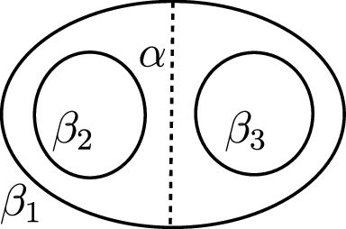
 $\alpha$
in Figure 2. The arc
 $\alpha$
cuts the boundary component
 $\beta_1$
into two arcs, the shortest one of which has length at most
 $({\ell(\beta_1)})/{2}\leq (({1+\delta})/{2})\ell(\beta_2)$
. If we suppose this shortest arc lies on the side of
 $\beta_2$
, we obtain
 $$\ell(\alpha) + \frac{1+\delta}{2}\ell(\beta_2) \geq \ell(\beta_2),$$
which gives us
 $\ell(\alpha) \geq (({1-\delta})/{2})\ell(\beta_2)\geq (({1-\delta})/{2})L $
and hence
 $$\mathrm{sys}(T_\phi) \geq (1-\delta)\cdot L \gt \ell.$$
A pair of pants.

We prove item (2) using essentially the same argument. Indeed, if a collar of width u around one of the pants curves is not standard, then this yields a simple arc of length at most 2u between two points on the corresponding pants curve. This arc must be essential relative to its endpoints and, by the same argument as above, such an arc has length at least
 $\ell/2$
. So, the collars of width
 $\ell/4\gt w$
(by assumption C3) are standard.
Finally, item (3) follows from the first part of the same assumption C3, combined with Proposition 4.2.
6.3 Strong convergence
To obtain covers of
 $X_B$
whose spectral gap is nearly optimal we will rely on the techniques developed by Hide and Magee [Reference Hide and MageeHM23, Reference Louder, Magee and HideLMH25] based on strong convergence of permutation representations.
Let
 $\Gamma$
be a finitely generated group and suppose
 $(\mathcal{H}_n)_n$
is a sequence of Hilbert spaces. Given a sequence of unitary representations
 $\rho_n:\Gamma \to U(\mathcal{H}_n)$
, where
 $U(\mathcal{H}_n)$
denotes the unitary group of
 $\mathcal{H}_n$
, we say that this sequence strongly converges to
 $\rho_{\infty}:\Gamma \to U(\mathcal{H}_\infty)$
if
 $$\lim_{n\to\infty} \| \rho_n(z) \| = \| \rho_\infty(z) \|$$
for all
 $z\in\mathbb{C}[\Gamma]$
.
We will need the following result which is a version of the results in [Reference MageeMag24b], specialized to our set-up.
Theorem 6.2.
Let
 $\Gamma\lt\textrm{PSL}(2,\mathbb{R})$
be a uniform lattice and let
 $\Lambda$
be a group. Moreover, suppose that:
-
–
$p:\Gamma \to \Lambda$
is an epimorphism and write
$K=\ker(p) \triangleleft \Gamma$
; -
–
$ (\rho_n\in \mathrm{Hom}(\Lambda,\mathfrak{S}_n) )_{n\geq 1}$
is a sequence of permutation representations such that where
$$\mathrm{std}_n\circ \rho_n \stackrel{\mathrm{strong}}{\longrightarrow} \rho_{\mathrm{reg}} \quad \text{as }n\to\infty,$$
$\mathrm{std}_n:\mathfrak{S}_n \to U(\mathbb{C}^{n-1})$
denotes the
$(n-1)$
-dimensional irreducible representation and
$\rho_{\mathrm{reg}}:\Lambda\to \mathcal{B}(\ell^2(\Lambda))$
denotes the left regular representation; and
-
– we can write
$\Gamma_n = \mathrm{Stab}_{\rho_n\circ p}(\{1\}) \lt \Gamma$
.


Then
 $$\lim_{n\to\infty}\lambda_1(\Gamma_n\backslash\mathbb{H}^2) = \min \{\lambda_1(K\backslash\mathbb{H}^2),\lambda_1(\Gamma\backslash \mathbb{H}^2) \}.$$
Proof sketch. This statement can be derived using small modifications of the arguments in [Reference Hide and MageeHM23, Reference Louder, Magee and HideLMH25, Reference Magee and ThomasMT26]. A representation-theoretic argument due to Magee [Reference MageeMag24b] is perhaps the fastest way to obtain it. Indeed, our statement is a special case of [Reference MageeMag24b, Theorem 3.1], which is phrased in a different language. We will very briefly describe how this works here.
The fact that
 $\mathrm{std}\circ \rho_n \stackrel{\text{strong}}{\longrightarrow} \rho_{\mathrm{reg}}$
, implies that
 $$\mathrm{std}_n\circ \rho_n \circ p \stackrel{\text{strong}}{\longrightarrow} \rho_{\mathrm{reg}}\circ p : \Gamma \to \mathcal{B}(\ell^2(\Lambda)).$$
Magee [Reference MageeMag24b, Theorem 3.1] proves that this implies that
 $$\mathrm{Ind}_\Gamma^{\textrm{PSL}(2,\mathbb{R})} (\mathrm{std}_n\circ \rho_n \circ p ) \stackrel{\text{strong}}{\longrightarrow} \mathrm{Ind}_\Gamma^{\textrm{PSL}(2,\mathbb{R})} (\rho_{\mathrm{reg}}\circ p ) .$$
By [Reference MageeMag24b, Proposition 2.9], this implies our statement.
Strongly convergent sequences of representations are notoriously hard to find. However, the following theorem by Bordenave and Collins [Reference Bordenave and CollinsBC19] gives us what we need.
Theorem 6.3 (Bordenave–Collins). Let F be a finitely generated non-abelian free group and let
 $\rho_n \in \mathrm{Hom}(F,\mathfrak{S}_n)$
be chosen uniformly at random. Then
 $$\mathrm{std}_n\circ \rho_n \stackrel{\mathrm{strong}}{\longrightarrow} \rho_{\mathrm{reg}} \quad \text{as }n\to\infty$$
in probability.
6.4 Covers of degree 2 and Hamming distance
Using good tree covers, combined with the existence of strongly convergent sequences of permutation representations of
 $F_2$
and Theorem 6.2 above, we can already use our construction to build sequences of finite covers of
 $X_B$
whose spectral gaps are arbitrarily close to
 $\frac{1}{4}$
. As such, we need to explain how to get intermediate spectral gaps.
As mentioned in § 1.1 of the proof strategy in the introduction, we will use a variation of the switching argument of Magee in order to do this. We will fix a homeomorphism
 $\phi:X_B\to X_B$
such that
 $T_\phi$
has satisfies the result from Proposition 6.1. This gives us a sequence
 $(Y_\phi^{(n)}\to X_B)_{n\geq 1}$
of random degree n covers (see § 2.3). The spectral gaps of
 $Y_\phi^{(n)}$
converge to that of
 $T_\phi$
in probability. We will further condition on
 $Y_\phi^{(n)}$
not having any short (to be quantified below) curves. We claim that this suffices for the set of spectral gaps of the degree 2 coversFootnote
4
 $\widehat{Y}\to Y_\phi^{(n)}$
to become arbitrarily dense in
 $[0,\lambda_0(T_\phi)]$
. The rest of this text is devoted to working this out.
First of all, we will restrict to covers that factor through the handlebody attachment. That is, the groups defined in § 2.3 fit in the commutative diagram

which allows us to define the set
 $$\mathcal{H}_\phi^{(n)} = \{ \rho\circ(\iota\circ\phi)_* : \rho\in\textrm{Hom}(H^{(n)},\mathbb{Z}/2\mathbb{Z})\}.$$
Given a free generating set
 $S=(s_1,\ldots,s_k)$
of
 $H^{(n)}$
, we can identify the set of maps
 $\mathcal{H}_\phi^{(n)}$
with
 $(\mathbb{Z}/2\mathbb{Z})^k$
through the map that associates
 $(\rho(s_1),\ldots,\rho(s_k))$
to
 $\rho\circ (\iota \circ\phi)_* \in \mathcal{H}^{(n)}_\phi$
. This in turn allows us to define a Hamming distance
 $\mathrm{d}_S:\mathcal{H}_\phi^{(n)} \times \mathcal{H}_\phi^{(n)} \to \mathbb{N}$
by
 $$\mathrm{d}_S (\rho_1\circ(\iota\circ\phi)_*,\;\rho_2\circ(\iota\circ\phi)_* ) = | \{ j : \rho_1(s_j)\neq \rho_2(s_j)\} |.$$
We note that every element
 $\rho\in\mathcal{H}_\phi^{(n)}$
corresponds to a cover of
 $Y_\phi^{(n)}$
. If the image of
 $\rho$
is trivial, we will let this cover be the cover of
 $Y_\phi^{(n)}$
by two disjoint copies of itself. This way, all the corresponding covers are of degree 2.
6.5 Switching
In this section we describe how two covers of degree 2 of
 $Y_\phi^{(n)}$
whose Hamming distance is 1 differ from each other.
To make this precise, we need to first describe a free generating set of
 $H^{(n)}$
. One way to do this is to identify
 $F_2$
with the fundamental group of a graph
 $W^{(1)}$
. We will let
 $W^{(1)}$
be a wedge of two circles. Because the pants curves in
 $\mathcal{P}_0$
are meridians, we can set everything up in such a way that the two edges of
 $W^{(1)}$
are dual to two of the pants curves in the pants decomposition
 $\mathcal{P}_0$
we have fixed. If we change the handlebody attachment by a homeomorphism
 $\phi:X_B\to X_B$
, this changes the identification. That is, we can think of the edges of
 $W^{(1)}$
as corresponding to two of the three pants curves in
 $\phi^{-1}(\mathcal{P}_0)$
. Here
 $H^{(n)}$
is the fundamental group of a graph
 $W^{(n)}$
that covers
 $W^{(1)}$
. The edges in this graph are dual to the canonical pants decomposition of
 $Y_\phi^{(n)}$
.
In order to obtain a preferred free generating set of
 $H^{(n)}$
, we pick an arbitrary spanning tree in
 $W^{(n)}$
and contract it. The edges that do not appear in the tree yield a generating set
 $S^{(n)}=(s_1,\ldots,s_k)$
of
 $H^{(n)}$
. Because of the correspondence between edges and pants curves described above, each of these generators is dual to a pants curve in the canonical pants decomposition of
 $Y_\phi^{(n)}$
. We will denote these preferred pants curves by
 $(\alpha_1^{(n)},\ldots,\alpha_k^{(n)})$
.
Given a map
 $\rho:H^{(n)}\to \mathbb{Z}/2\mathbb{Z}$
, the corresponding cover of degree 2 of
 $Y_\phi^{(n)}$
can be built as follows.
-
– Write
$Z_\phi^{(n)} = \overline{Y_\phi^{(n)} - \bigcup_{i=1}^k\alpha_i}$
, where
$\overline{X}$
denotes the completion of a hyperbolic surface X, so
$Z_\phi^{(n)}$
is a surface with boundary. -
– Take two disjoint copies
$Z_1$
and
$Z_2$
of
$Z_\phi^{(n)}$
. -
– Then, for each pants curve
$\alpha_i$
:-
* if
$\rho(s_i) = [0]$
, glue the two boundary components of
$Z_1$
corresponding to
$\alpha_i$
back together and do the same for those in
$Z_2$
; -
* if
$\rho(s_i) = [1]$
, glue the ‘left’ boundary component of
$Z_1$
corresponding to
$\alpha_i$
to the ‘right’ boundary component of
$Z_2$
and, likewise, glue the corresponding right boundary component of
$Z_1$
to the left boundary component of
$Z_2$
.
-


All these gluings above should be performed with the correct twist, so as to guarantee that the resulting surface covers
 $Y_\phi^{(n)}$
.
It follows from this description that if
 $$\mathrm{d}_{S^{(n)}} ( \rho_1 \circ (i\circ \phi)_*,\; \rho_2 \circ (i\circ \phi)_* ) =1,$$
then the two corresponding covers can be obtained from each other by opening up the lifts corresponding to one of the preferred pants curves
 $\alpha_i^{(n)}\subset Y_\phi^{(n)}$
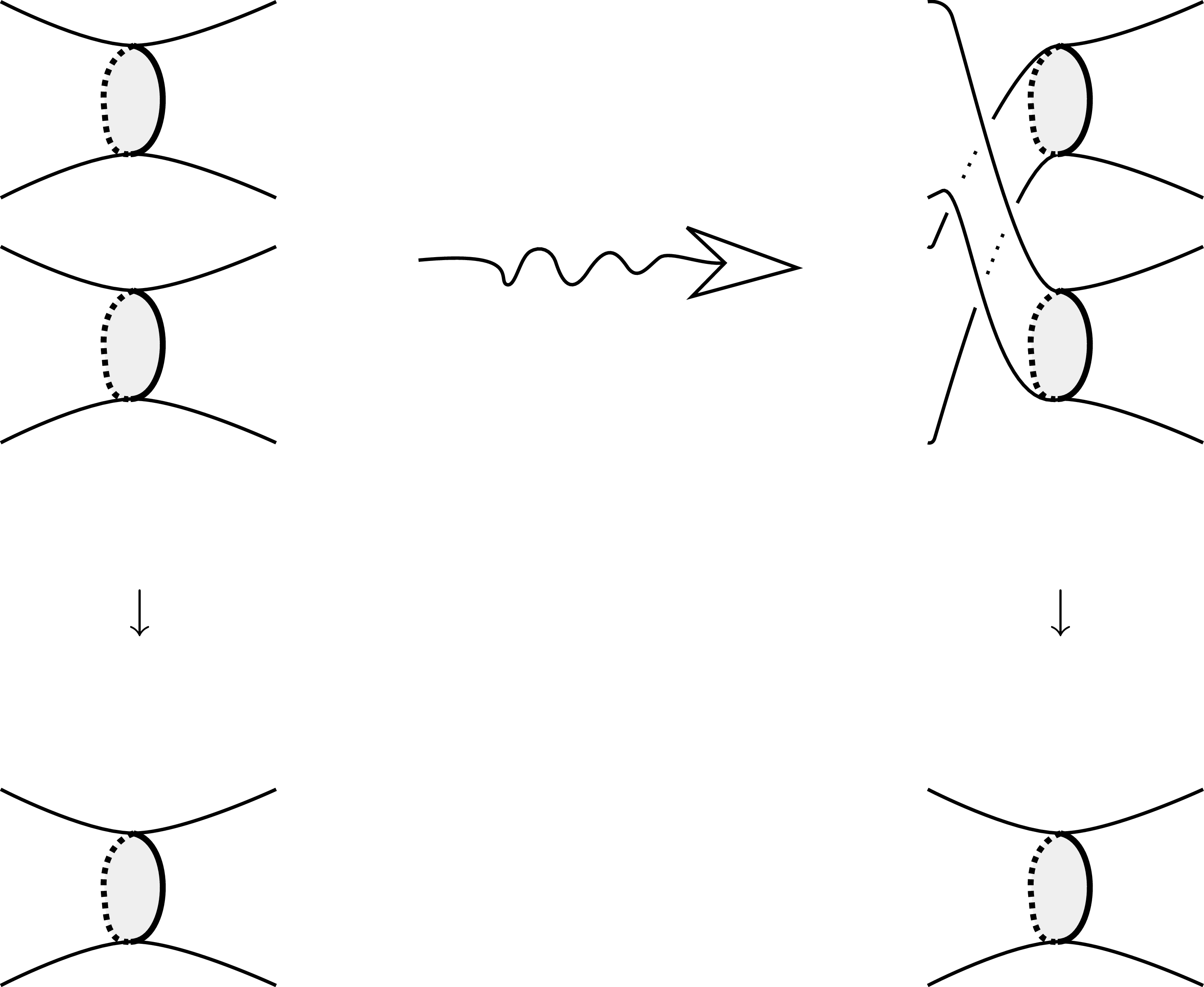
and gluing them back together with the opposite pattern. We will call this operation a switch; this same terminology is used in graph theory for what happens at the level of the 2-covers of the graph
 $W^{(n)}$
. Figure 3 shows a local picture of this move.
A local picture of a switch. The surface at the bottom represents a neighbourhood of one of the preferred pants curves
 $\alpha_i^{(n)}$
of
 $Y^{(n)}_\phi$
. The surfaces at the top (one on the left and one on the right) are the neighbourhoods of the lifts of
 $\alpha_i^{(n)}$
in two distinct covers of degree 2. The shading is there to indicate that the curves that are involved are meridians.

6.6 Finishing the proof
We now have everything we need in place to finish the proof of our main theorem. Indeed, Theorem 1 is implied directly by the following result.
Theorem 6.4.
For all
 $n\in\mathbb{N}$
large enough, the probability that the set
 $$\{ \lambda_1(\widehat{Y}) : \widehat{Y} \text{ is a connected cover of }Y_\phi^{(n)} \text{ of degree 2}\}$$
is
 $\eta$
-dense in
 $[0,\frac{1}{4}]$
, is strictly positive.
Proof. First of all, we use Proposition 6.1 to choose a homeomorphism
 $\phi:X_B\to X_B$
that gives us a tree cover with the properties in that same proposition.
It now follows from Theorems 6.2 and 6.3 that
 $\lambda_1(Y_\phi^{(n)}) \gt \frac{1}{4}-\eta$
with high probability. In fact, using the same argument as in [Reference MageeMag24a, § 4],
 $$\theta\otimes\rho_n \stackrel{\text{strong}}{\longrightarrow} \rho_{\mathrm{reg}}$$
in probability as
 $n\to\infty$
, for any
 $\theta\in\textrm{Hom}(F_2,\mathbb{Z}/2\mathbb{Z})$
. For us this means that, again using Theorem 6.2, we obtain covers of degree 2, corresponding to some element in
 $\mathcal{H}^{(n)}_\phi$
, of
 $Y_\phi^{(n)}$
whose spectral gap is at least
 $$\lambda_1(T_\phi) - \eta/2 \gt \tfrac{1}{4}-\eta$$
for n large enough.
The set
 $\mathcal{H}^{(n)}_\phi$
also contains the trivial homomorphism, the corresponding degree 2 cover of which has
 $\lambda_1(\widehat{Y})=0$
.
We can go between these covers using a finite number of switches, so as soon as we prove that a single switch does not change the spectral gap by more than
 $\eta$
, we are done.
In order to do this, we need to make one further assumption on the surfaces
 $Y^{(n)}$
: the preferred pants curves in
 $Y^{(n)}$
need to have collar width at least w and the systole of
 $Y^{(n)}$
needs to be at least
 $\ell$
.
Both of these statements are true in the tree cover
 $T_\phi$
. This means, that if they are not true in
 $Y^{(n)}$
, there needs to be a closed geodesic
 $\gamma\subset X_B$
of uniformly bounded length
 $L=L(w,\ell)$
such that
 \begin{equation}\iota_*(\gamma) \neq e \quad \text{but} \quad \rho_n\circ (\iota\circ\phi)_*(\gamma) \cdot 1 = 1.\end{equation}
It follows from Nica’s work [Reference NicaNic94] that, with asymptotically strictly positive probability,
 $\rho_n(g)$
is fixed-point-free for all g in any fixed finite set of non-trivial conjugacy classes in
 $F_2$
. The statement we use here is as follows. First of all, let
 $K_1,\ldots K_m\subset F_2$
be a finite collection of distinct non-trivial conjugacy classes, none of which contain a power of a non-trivial element of
 $F_2$
. Moreover, let
 $(c_1,\ldots,c_k)$
be a finite set of cycle lengths. Then the vector of random variables
 $ (X_{c_i}(K_j) )_{1\leq i \leq m,\; 1\leq j\leq k}$
, where
 $X_{c_i}(K_j)$
denotes the number of
 $c_i$
-cycles in the image of an element of
 $K_j$
under a uniformly random homomorphism
 $\rho \in \textrm{Hom}(F_2,\mathfrak{S}_n)$
, converges in distribution to a vector of independent random variables. Furthermore, the limit of
 $X_{c_i}(K_j)$
is
 $\mathrm{Poisson}(1/c_i)$
-distributed. This statement is not literally contained in Nica’s paper, but it can be proven using similar methods. Versions of this statement are also available in [Reference Linial and PuderLP10, § 4], [Reference Baker and PetriBP23, Theorem 1.4] and [Reference Puder and ZimhoniPZ24, Corollary 1.7 and Theorem 1.14]. The only consequence we need is that there exists a uniform
 $a\gt0$
such that for all n large enough,
 $$\mathbb{P} (X_{c_i}(K_j) = 0\text{ for }i=1,\ldots,k \text{ and } j=1,\ldots,m ) \gt a.$$
Also observe that if
 $g = u^k\in F_2$
and if, under a permutation representation of
 $F_2$
, u has no d-cycles for any divisor d of k, then g has no fixed points.
Since
 $\Gamma_B$
contains a finite number of conjugacy classes of elements of bounded translation length, we can avoid the existence of a closed geodesic
 $\gamma\subset X_B$
as in (6.1) with strictly positive probability. Moreover, the existence of a 2-cover with spectral gap above
 $\frac{1}{4}-\eta$
has probability tending to 1 as
 $n\to \infty$
, so this property is preserved when we restrict to covers without short geodesics that do not lift to
 $T_\phi$
. In other words, the probability that
 $Y^{(n)}_\phi$
has systole at least
 $\ell$
, all the curves in the canonical pants decomposition have standard collars of width w and
 $Y^{(n)}_\phi$
has a 2-cover with spectral gap at least
 $\frac{1}{4}-\eta$
is asymptotically strictly positive.
So now suppose
 $\widehat{Y}_1$
and
 $\widehat{Y}_2$
are two covers of degree 2 of
 $Y_\phi^{(n)}$
that differ by a switch move. Moreover, let f be a
 $\lambda_1(\widehat{Y}_1)$
-eigenfunction on
 $\widehat{Y}_1$
and let
 $\alpha_i$
be the curve in which we need to switch to obtain
 $\widehat{Y}_2$
. Using Proposition 5.3, there exists a smooth function
 $f_1$
on
 $\widehat{Y}_1$
of zero average that is constant on a neighbourhood of both lifts of
 $\alpha_i$
and
 $$\frac{\langle \Delta f_1,f_1\rangle}{\langle f_1,f_1\rangle}-\lambda_1(\widehat{Y}_1) \leq 2B\ell \|f\|^2_{\infty}\leq 2AB\ell e^{-\ell\sqrt{\eta}} \leq \eta.$$
Here we have used Theorem 5.1 together with the assumption on the collar widths and the systole of
 $Y_\phi^{(n)}$
and the relations between our constants (§ 6.1). Because
 $f_1$
attains the same constant value on neighbourhoods of the lifts of
 $\alpha_i$
, it defines a function of zero average on the cover
 $\widehat{Y}_2$
and hence
 $$\lambda_1(\widehat{Y}_2) \leq \lambda_1(\widehat{Y}_1) + \eta,$$
by the variational characterization of
 $\lambda_1$
, which concludes the proof.
Acknowledgements
We are very grateful to Maxime Fortier Bourque for his part in developing the code that we use in § 3. We also thank the SageMath [Sag21], Arb [Reference JohanssonJoh17] and GAP [GAP22] developers for making the calculations using that same code possible.
We thank the CIRM for hosting the workshop Random Hyperbolic Surfaces and Random Graphs, part of the Jean-Morlet Chair semester Random Matrices, Representation Theory and Quantum Information, during which this project started.
We thank Michael Magee and Frédéric Naud for useful conversations surrounding this project. Finally, we thank the anonymous referee for helpful suggestions.
Conflicts of interest
None.
Financial support
BP was partially supported by the grant ANR-23-CE40-0020-02 ‘MOST’.
Data availability
The code for this article, which is used in the proof of Proposition 3.2, is available as supplementary material.
Journal information
Compositio Mathematica is owned by the Foundation Compositio Mathematica and published by the London Mathematical Society in partnership with Cambridge University Press. All surplus income from the publication of Compositio Mathematica is returned to mathematics and higher education through the charitable activities of the Foundation, the London Mathematical Society and Cambridge University Press.
Supplementary material
Supplementary material for this article is available at: https://doi.org/10.1017/S0010437X26103340.


 αi(n)
 Yϕ(n)
 αi(n)


 Open access

