


1. INTRODUCTION
When a plasma wakefield is driven to nonlinear amplitudes, it takes the form of an electronic cavity that is called “bubble” in the case of a short pulse laser driver (Pukhov & ter Vehn, Reference Pukhov and ter Vehn2002) or “blowout regime” in the case of dense highly energetic particle bunches (Rosenzweig et al., Reference Rosenzweig, Breizman, Katsouleas and Su1991; Lotov, Reference Lotov2004). For the laser driven case, the pulse is shorter than the plasma wavelength and fits perfectly into the first half of the plasma period. The laser intensity is thought to be high enough that the created wakefield breaks after its first oscillation. In this regime, the wakefield takes the form of a distorted spherical cavity from which all electrons are banished and that moves with nearly the speed of light through the plasma. In the following, we refer this wakefield as “the bubble”.
The physics of electron self-injection in a bubble is very complex. The modern theory of self-injection is still in an early stage as it cannot predict accurately quantities observed in experiments. In the last years, recent bubble models have been invented and most of them suggest their own criteria of electron trapping (Kostyukov et al., Reference Kostyukov, Nerush, Pukhov and Seredov2009; Reference Kostyukov, Nerush, Pukhov and Seredov2010; kalmykov et al., Reference Kalmykov, Beck, Yi, Khudik, Downer, Lefebvre, Shadwick and Umstadter2011; Reference Kalmykov, Beck, Davoine, Lefebvre and Shadwick2012; Yi et al., Reference Yi, Khudik, Kalmykov and Shvets2011; Reference Yi, Khudik, Siemon and Shvetsa2013; Lu et al., Reference Lu, Tzoufras, Joshi, Tsung, Mori, Vieira, Fonseca and Silva2007; Pak et al., Reference Pak, Marsh, Martins, Lu, Mori and Joshi2010; Zeng et al., Reference Zeng, Davidson, Lu, An, Sheng and Mori2012). The models in Kostyukov et al. (Reference Kostyukov, Nerush, Pukhov and Seredov2009; Reference Kostyukov, Nerush, Pukhov and Seredov2010) e.g., suggest that plasma electrons are self-injected in the bubble when the normalized bubble radius is approximately more than the Lorentz gamma-factor of the bubble rear. A modification of this criterion is proposed in Thomas (Reference Thomas2010). However, this modification has been seriously criticized in the comment of Corde et al. (Reference Corde, Stordeur and Malka2011) where mathematical correctness of the model presented in Kostyukov et al. (Reference Kostyukov, Nerush, Pukhov and Seredov2009; Reference Kostyukov, Nerush, Pukhov and Seredov2010) has been demonstrated. The semi-analytical model in Kalmykov et al. (Reference Kalmykov, Yi, Khudik and Shvets2009) suggest that electron self-injection occurs in the evolving bubble when the effective Hamiltonian becomes negative. This implies that the untrapped electrons cross the separatrix in the phase space, get into the bucket and become trapped. However, further analysis has shown (Yi et al., Reference Yi, Khudik, Kalmykov and Shvets2011) that the plasma electrons can also efficiently accelerated outside of the bucket. In recent advanced versions, the effect of the laser pulse evolution (Kalmykov et al., Reference Kalmykov, Beck, Davoine, Lefebvre and Shadwick2012) and the effect of the plasma sheath surrounding bubble (Yi et al., Reference Yi, Khudik, Siemon and Shvetsa2013) are included. Lu et al. have deduced from PIC simulations a simple criterion that electron self-injection can occur for the bubble above a threshold radius (laser intensity) that has a weak dependence on the bubble velocity (Lu et al., Reference Lu, Tzoufras, Joshi, Tsung, Mori, Vieira, Fonseca and Silva2007). In recent papers (Pak et al., Reference Pak, Marsh, Martins, Lu, Mori and Joshi2010; Zeng et al., Reference Zeng, Davidson, Lu, An, Sheng and Mori2012) the trapping condition is expressed through a wake pseudo-potential. The models we present in this paper are advanced versions of Kostyukov et al. (Reference Kostyukov, Nerush, Pukhov and Seredov2010) that unify analytical descriptiveness and self-consistent treatment of self-injection physics.
In a pure analytical model, we can calculate the fields inside the bubble from Maxwell's equations for an empty sphere (Kostyukov et al., Reference Kostyukov, Pukhov and Kiselev2004) and a sphere that takes into account the field enhancement at the bubble back due to electron sheet crossing (Bulanov et al., Reference Bulanov, Pegoraro, Pukhov and Sakharov1997; Lu et al., Reference Lu, Tzoufras, Joshi, Tsung, Mori, Vieira, Fonseca and Silva2007). An even simpler model for the fields inside the bubble has been proposed recently: a static piecewise model (PWM) (Kostyukov et al., Reference Kostyukov, Nerush, Pukhov and Seredov2010). This simplified model neglects any spatial or temporal field dependence, but due to its simplicity it is possible to calculate amplitude envelope functions to the transverse particle coordinates and momenta, and to analyze some self-injection physics. In contrast to recent experiments (Lu et al., Reference Lu, Tzoufras, Joshi, Tsung, Mori, Vieira, Fonseca and Silva2007; Wang et al., Reference Wang, Zgadzaj, Fazel, Li, Yi, Zhang, Henderson, Chang, Korzekwa, Tsai, Andn Pal, Quevedo, Dyer, Gaul, Martinez, Bernstein, Borger, Spinks, Donovan, Khudik, Shvets, Ditmire and Downer2013), the PWM misses the production of mono energetic electron beams. Thus, we are forced to modify the PWM to a more general case that remains analytically treatable and improves the self-injection physics found in the PWM.
Our first approach is to consider fields that are time dependent, but piecewise constant in space. In this case, our model is a sphere with an adiabatically growing radius R(t) and a growing trapping cross-section. A physical justification for this approach is that now the interaction of the electron bunch with the bubble border is taken into account. Since the fields remain constant we still miss the production of mono energetic electron beams. Thus, in a second step we introduce a model that treats the right field gradient in the longitudinal direction. For this case indeed, we find energy spectra that are comparable to PIC simulations and a full gradient model.
Our work is based on the PWM. Thus, similar to Kostyukov et al. (Reference Kostyukov, Nerush, Pukhov and Seredov2010), our bubble models neglect the interaction between the accelerated electrons and the laser pulse at the bubble front. We also assume a continuous plasma background density, and a reduced electron dynamics in the z-ρ-plane, where ρ is the perpendicular distance of an electron to the z-axis and z the propagation direction of the laser pulse. The motivation for all these assumptions are several observations in the phenomenological model of the bubble regime (Kostyukov et al., Reference Kostyukov, Pukhov and Kiselev2004; Reference Kostyukov, Nerush, Pukhov and Seredov2009).
The full gradient potentials inside a bubble are given in Kostyukov et al. (Reference Kostyukov, Pukhov and Kiselev2004) and Lu et al. (Reference Lu, Huang, Zhou, Tzoufras, Tsung, Morl and Kat- Souleas2006) In normalized variables, they are A ‖ = −φ = Φ/2, and A⊥ = 0, where Φ(r) = |r|2/4 is the bubble potential. The normalization is done by r → rωpe/c for length, t → tωpe for time, v → v/c for velocity, p → p/(m ec) for the kinetic momentum, and Φ → eΦ/(m ec 2) for potentials. Here ωpe = (4πe 2n 0/m e)1/2 is the electron plasma frequency, m e is the electron mass, c is the velocity of light, and n 0 is the plasma background density. The equations of motion of the full gradient model in a co-moving frame of reference are Eq.(1)–(2) in Kostyukov et al. (Reference Kostyukov, Nerush, Pukhov and Seredov2009). In the PWM, ξ = z − Vt and ρ are replaced by
 $${\rm \xi} = {\rm sgn}\lpar {\rm \xi} \rpar F\comma \; \quad {\rm \rho} = {\rm sgn}\lpar {\rm \rho} \rpar F\comma \;$$
where F is the field-strength parameter of the PWM and V the group velocity of the laser pulse.
2. THE TIME-DEPENDENT PWM (TPWM)
One possibility to examine the interaction between the electron bunch and the bubble border is to consider an adiabatically slow bubble growth. This growth significantly affects the electron self-injection physics because the bubble moves back slower than the bubble (Kostyukov et al., Reference Kostyukov, Pukhov and Kiselev2004; Reference Kostyukov, Nerush, Pukhov and Seredov2009; Whittum, Reference Whittum1992; Lu et al., Reference Lu, Tzoufras, Joshi, Tsung, Mori, Vieira, Fonseca and Silva2007; Kalmykov et al., Reference Kalmykov, Yi, Khudik and Shvets2009; Yi et al., Reference Yi, Khudik, Kalmykov and Shvets2011; Kalmykov et al., Reference Kalmykov, Beck, Yi, Khudik, Downer, Lefebvre, Shadwick and Umstadter2011).
To adopt the idea of a growing bubble to the tPWM we make the same consideration as in Kalmykov et al. (Reference Kalmykov, Yi, Khudik and Shvets2009) and Yi et al. (Reference Yi, Khudik, Kalmykov and Shvets2011). Applied to the full gradient model (Kostyukov et al., Reference Kostyukov, Pukhov and Kiselev2004), we find the sufficient trapping condition limt→∞Φ(t) = −∞. Thus, a new approach for our wakefield potential in the tPWM is
 $$\Phi \lpar {\bf r}\comma \; t\rpar = \displaystyle{F \over 2}\lpar \vert {\rm \xi} ^ - \vert + \vert {\rm \rho} \vert \rpar - \displaystyle{{R\lpar t\rpar ^2 } \over 4}\comma \;$$
with R(t) = (1 + ϵt)R 0, ξ− = z − V −t, V − = V − ϵR 0, 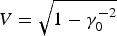 $V = \sqrt {1 - {\rm \gamma}_0^{ - 2} }$, and the gamma-factor of the bubble front γ0. In these coordinates, the bubble center rests and the equations of motion for the tPWM are
 $$\displaystyle{{dp_{\vert \vert } } \over {dt}} = - \displaystyle{1 \over 4}\Omega ^ - + \displaystyle{{{\rm sgn}\lpar {\rm \rho} \rpar Fp_ \bot } \over {4{\rm \gamma}}}\comma \;$$
 $$\displaystyle{{dp_ \bot } \over {dt}} = - \left({1 + \displaystyle{{\,p_{\vert \vert } } \over {\rm \gamma}}} \right)\displaystyle{{{\rm sgn}\lpar {\rm \rho} \rpar F} \over 4}\comma \;$$
 $$\displaystyle{{d{\rm \xi} ^ - } \over {dt}} = \displaystyle{{\,p_{\vert \vert } } \over {\rm \gamma}} - V^ - \comma \; \quad \displaystyle{{d{\rm \rho} } \over {dt}} = \displaystyle{{\,p_ \bot } \over {\rm \gamma}}\comma \;$$
with Ω− = (1 + V −)sgn(ξ−)F + (1 + ϵt)R 02ϵ.
Based on the tPWM we perform two kinds of simulation. In the first part, we solve the equations of motion (3)–(5) for a single electron and discuss its trajectory, while we always assume the initial conditions (ξ0−)2 + ρ02 = R 02, p0 = 0, and ϵ, ξ0−, ρ0 > 0. In the second part we place a grid of particles with zero momentum in front of the bubble as shown in Figure 1c and solve the equations of motion for every individual particle. The resulting energy spectra of trapped particles then give us a better insight in the self injection dynamics and acceleration mechanism in the tPWM.
(Color online) (a) Trajectory in the PWM, particle is not trapped. (b) Trajectory in the tPWM, particle is trapped. Both simulations are done with R 0 = 5, F = 4, ρ0 = 4.92, and γ0 = 10. The black solid circle has radius R 0. The blue dotted circle is the bubble after the simulation ends. (c): Simulation configuration: Bubble running into a grid of electrons.

If we compare a particle's trajectory in both the PWM (Figure 1a) and the tPWM (Figure 1b), we discover a new kind of trapping dynamic. The particle in the static model is lost because its trajectory crossed the bubble border. In the time-dependent model, this situation can be prevented as the border moves out. The amplitude function of the oscillation in the trajectory determines whether the electron will be trapped. So, Kostyukov et al. (Reference Kostyukov, Nerush, Pukhov and Seredov2010) describe a way to calculate the envelope approximation functions  $\tilde {\rm \rho} \lpar t\rpar $ and
 $\mathop {\tilde p}\nolimits_ \bot \lpar t\rpar $ to the amplitude functions of ρ(t) and p ⊥(t). We follow their steps in the limit ϵR 02≪2F and introduce the times t n by ρ(t n) = 0 for all n ≥ 1. Then, with n≫1 and a guiding center approximation to p ‖(t), we obtain the equation system
 $$\mathop {\tilde p}\nolimits_{\vert \vert } \lpar t\rpar = \displaystyle{1 \over 4}[ \lpar 1 + V^ - \rpar F - R_0^2 {\rm \epsilon}] t\comma \;$$
 $$\mathop {\tilde p}\nolimits_ \bot \lpar t\rpar = 1.00\tilde cy_0^{2/3} \displaystyle{{F^{5/3} } \over {\vert \Omega ^ - \lpar t\rpar \vert }}[ \lpar 1 + V^ - \rpar F - R_0^2 {\rm \epsilon}] ^{1/3} t^{1/3}\comma \;$$
 $$\tilde {\rm \rho} \lpar t\rpar = 4.01\displaystyle{{\mathop {\tilde c}\nolimits^2 {\rm \rho} _0^{4/3} F^{7/3} } \over {\Omega ^ - \lpar t\rpar ^2 [ \lpar 1 + V^ - \rpar F - R_0^2 {\rm \epsilon}] ^{1/3} }}t^{ - 1/3}\comma \;$$
while we use the constant  $\tilde c = \tilde c\lpar F\comma \; R_0 \comma \; {\rm \gamma} _0 \comma \; {\rm \epsilon}\comma \; {\rm \xi} _0^ - \rpar $ to fit the curves to our simulations.
Two exemplary plots of the envelope functions  $\mathop {\tilde p}\nolimits_ \bot \!\!\lpar t\rpar $ and
 $\mathop {\tilde p}\nolimits_ \bot \!\!\lpar t\rpar $ (red dotted lines) together with the simulated coordinate and momenta of a particle (blue solid lines) are shown in Figure 2. The analytical predictions are in good agreement with the simulations and converge very close to the actual enveloping functions.
(Color online) (a, b): Envelope approximation functions (red dotted lines) and numerical solutions (blue solid lines) to ρ(t) and p ⊥(t) in the tPWM. The simulation parameters are F = 4, R 0 = 6, γ0 = 10, and ε = 0.0004. (c): Trapping cross-sections from analytical prediction (blue line) and numerical simulations (red circles) for γ0 = 10, ε = 0.0002, and F = 6 in the tPWM.
To calculate the trapping conditions, we demand |r|2 = (ξ−)2 + ρ2 < R 2 and show that for n≫1
 $${\rm \xi} _0^ - \lt - \displaystyle{2 \over F} + \displaystyle{{R_0 F^{3/4} \mathop {\tilde c}\nolimits^{3/2} } \over {\lpar F - R_0^2 {\rm \epsilon}\rpar ^{3/4} {\rm \gamma} _0^{1/2} }}\left({1.48 + 0.72\displaystyle{{R_0 {\rm \epsilon}{\rm \gamma} _0^2 F} \over {2F - R_0^2 {\rm \epsilon}}}} \right)\comma \;$$
is the condition that must hold to trap electrons. From Eq.(9) and ρ02 = R(t)2 − (ξ0−)2 we calculate the trapping cross section σ = π(R 2 − ρmin2) with ρmin = min ρ0. If we assume ΔR = R − ρmin = const, we find that σ(t) is linearly time-dependent. To confirm our estimation, we plot log(σ) and log(R 0) into one diagram (see Figure 2c). As we observe, the analytical prediction (blue line) follows the numerically found trapping cross sections (red circles) and stays especially for large R 0 in a 5% error range.
To analyze the energy spectra in the tPWM a grid of electrons with zero momentum is placed in front of the bubble (see Figure 1c). Afterward, we solve the equations of motion for every individual particle, i.e., we neglect the interaction of the test electrons. The electron spectra we receive after the electron bunch of trapped electrons has passed its acceleration length look like that in Figure 3a. Here, we don't observe any mono energetic electron beams but a quasi equal distribution of the particles' energy. Apparently, this contradicts pic simulations results as shown in Figure 3b and experiments (Hidding et al., Reference Hidding, Amthor, Liesfeld, Schwoerer, Karsch, Geissler, Veisz, Schmid, Gallacher, Jamison, Jaroszynski, Pretzler and Sauerbrey2006; Mangles et al., Reference Mangles, Murphy, Najmudin, Thomas, Coller, Dangor, Divall, Foster, Gallacher, Hooker, Jaroszynski, Langley, Mori, Norreys, Tsung, Viskup, Walton and Krushelnick2004; Faure et al., Reference Faure, Glinec, Pukhov, Kiselev, Gordienko, Lefebvre, Rousseau, Burgy and Malka2004; Lu et al., Reference Lu, Tzoufras, Joshi, Tsung, Mori, Vieira, Fonseca and Silva2007; Wang et al., Reference Wang, Zgadzaj, Fazel, Li, Yi, Zhang, Henderson, Chang, Korzekwa, Tsai, Andn Pal, Quevedo, Dyer, Gaul, Martinez, Bernstein, Borger, Spinks, Donovan, Khudik, Shvets, Ditmire and Downer2013).
(Color online) (a) Energy distribution for F = 4, R 0 = 4, ε = 0.004, and γ0 = 5 in the tPWM. (b) PIC energy spectra taken from Figure 2 in Pukhov and Gordienko (Reference Pukhov and Gordienko2006). (c) Energy spectra in the hPWM for γ0 = 15, R 0 = 8, and F = 4.
The monoenergetic spectra can be recovered in the full gradient model. Thus, in the following section we introduce another extension of the PWM that is still analytically treatable and preserves a production of mono energetic electron beams.
3. THE HALF-GRADIENT PWM (HPWM)
In the hPWM, we still replace the perpendicular field E ⊥ by the constant field-strength parameter F. In longitudinal direction, however, we take the full field gradient. The resulting wakefield potential is
 $$\Phi \lpar {\bf r}\rpar = \displaystyle{{{\rm \xi} ^2 + 2F\vert {\rm \rho} \vert } \over 4} - \displaystyle{{R_0^2 } \over 4}.$$
Here, the coordinate ξ = z − Vt always contains the group velocity of the generating laser pulse at the bubble front because the bubble radius is fixed.
If we repeat the simulations of the electron grid in the the hPWM, we get energy spectra similar to those shown in Figure 3. As we see, both PIC-simulated spectra in Figure 3b and our spectrum from a simulation with F = 4, R 0 = 8, and γ0 = 15 exhibit the same structure. Since the hPWM is able to describe the production of monoenergetic electron beams, we calculate the equations of motion
 $$\displaystyle{{dp_{\vert \vert } } \over {dt}} = - \Omega + \displaystyle{{\,p_ \bot } \over {\rm \gamma}}\displaystyle{{{\rm sgn}\lpar {\rm \rho} \rpar } \over F}4\comma \;$$
 $$\displaystyle{{dp_ \bot } \over {dt}} = - \left({1 + \displaystyle{{\,p_{\vert \vert } } \over {\rm \gamma}}} \right)\displaystyle{{{\rm sgn}\lpar {\rm \rho} \rpar F} \over 4}\comma \;$$
 $$\displaystyle{{d{\rm \xi} } \over {dt}} = \displaystyle{{\,p_{\vert \vert } } \over {\rm \gamma}} - V\comma \; \quad \displaystyle{{d{\rm \rho} } \over {dt}} = \displaystyle{{\,p_ \bot } \over {\rm \gamma}}\comma \;$$
with Ω = (1 + V)ξ/4. A simple form for the envelope approximation functions to ρ(t) and p⊥(t) can be found, if we express them in terms of τ = t − t max, where ξ(t max) = 0. For the calculation, we follow Kostyukov et al. (Reference Kostyukov, Nerush, Pukhov and Seredov2010) again and assume γ(t) ≪ 2(n cr/n 0)2 for all t for the electron energy. Then we have
 $$\mathop {\tilde p}\nolimits_{\vert \vert } \lpar {\rm \tau} \rpar \approx p_{max} - \displaystyle{{\lpar 1 + V\rpar } \over {16{\rm \gamma}_0^2 }}{\rm \tau} ^2\comma \;$$
 $$\mathop {\tilde p}\nolimits_ \bot \lpar {\rm \tau} \rpar = \sqrt \Lambda \lpar F\mathop {\tilde p}\nolimits_{\vert \vert } \lpar {\rm \tau} \rpar \rpar ^{1/3}\comma \;$$
 $$\tilde {\rm \rho} \lpar {\rm \tau} \rpar = \Lambda \lpar F\mathop {\tilde p}\nolimits_{\vert \vert } \lpar {\rm \tau} \rpar \rpar ^{ - 1/3}\comma \;$$
with Λ = 21/3C(t n)2/8Ω(t n)2. As in the previous section, the constant C(t n) is used to fit our approximations to numerical simulations.
To compare the approximated functions to the actual amplitude envelope functions, we solve the equations of motion for a single electron with initial conditions ξ02 + ρ02 = R 02, p0 = 0, and ξ0, ρ0 > 0. An exemplary plot of Eqs.(15)–(16) together with numerical solutions is shown in Figure 4. The analytical predictions (red dotted lines) are in good agreement to the simulations (black solid lines) and converge very close to the actual enveloping functions.
(Color online) Envelope approximation functions (red dotted lines) and numerical solutions (blue solid lines) to ρ(t) and p ⊥(t) in the hPWM. The simulation parameters are F = 5, R 0 = 10, and γ0 = 20.
Similar to Eqs.(9) the self-injection physics is described by the limiting condition
 $${\rm \rho} _{{\rm min}} = F + \mathop {\left({4 + F^2 - \displaystyle{{2P_0 } \over {{\rm \gamma} _0^2 }} - \displaystyle{{2\Lambda F^{2/3} } \over {P_0^{1/3} }} + \displaystyle{{\Lambda ^2 } \over {\lpar FP_0 \rpar ^{2/3} }}} \right)}\nolimits^{1/2}\comma \;$$
together with
 $$P_0^{5/3} - \displaystyle{{{\rm \gamma}_0^2 \Lambda F^{2/3} } \over 3}P_0^{1/3} + \displaystyle{{{\rm \gamma}_0^2 \Lambda ^2 F^{ - 2/3} } \over 3} = 0.$$
The trapping cross-section σ = π(R 02 − ρmin2) is constant in time since R 0 and ρmin are. If we plot σ and R 0 into one diagram (see Figure 5a), we observe that for a large range of parameters the accuracy remains in a 1% range.
(Color online) (a) Trapping cross-section for F = R 0/2. (b) Maximal applicable F. Both figures are simulated with γ0 = 15 and belong to the hPWM.
To get some analytical expressions for the limits of the bubble parameters, the so called trapping conditions, we start again with Eq.(17) and demand ρmin < R 0. Then we find after some algebraic transformations
 $$\eqalign{{\rm \gamma}_0^2 \lt 2P_0 \lpar 2FR_0 - R_0^2 + 4 - 2\Lambda F^{2/3} P_0^{ - 1/3} + \Lambda ^2 F^{ - 2/3} P_0^{ - 2/3} \rpar ^{ - 1}\comma \;}$$
as well as
 $$F^{5/3} - \displaystyle{\Lambda \over {R_0 P_0^{1/3} }}F^{4/3} + \left({\displaystyle{2 \over {R_0 }} - \displaystyle{{R_0 } \over 2} - \displaystyle{{P_0 } \over {R_0 {\rm \gamma} _0^2 }}} \right)F^{2/3} - \displaystyle{{\Lambda ^2 } \over {P_0^{2/3} }} \lt 0.$$
These two equations give us all parameter limits for the hPWM. To demonstrate that these complicated-looking limits are indeed well calculated we plot the largest F for which still an electron is trapped against R 0 in a simulation with one electron (compare former sections) in Figure 5b. As we see the analytical found F max (blue line) fits perfect to our simulations (red dots).
4. CONCLUSION
Summarizing our expansions of the original PWM we note two things. First, we see that it is possible to treat an enhanced interaction between the electron bunch and the bubble potentials. This in turn leads to a growing trapping cross-section and thus to a more efficient self-injection.
Energy spectra in our simulations show that no mono energetic electron beams are generated, if all field gradients are neglected. To fix this problem, we invent a hybrid model that includes the right fields in moving direction and replaces the transverse field gradients by a field strength parameter. In this modification, we observe the generation of mono energetic electron beams and are able to calculate trapping conditions analytically.
The next steps of our work will be to go back to the original full gradient model and to try to find the envelope approximation functions by other means than the introduction of a field strength parameter. If we succeed, we will have a fully-analytical model at hand that predicts trapping cross-sections and trapping conditions and that is directly comparable to computer simulations and experiments.
ACKNOWLEDGMENTS
This work has been supported by the Deutsche Forschungsgemeinschaft via GRK 1203 and SFB TR 18. This work has been supported by EU EuCARD-2 and ANAC2 -projects. This work has been supported by the Ministry of Education and Science of the Russian Federation No 14.B25.31.0008, by RFBR No 13-02-00886, by the Ministry of Science and Education of the Russian Federation, the Russian Federal Program “Scientific and scientific-pedagogical personnel of innovative Russia” (Agreement No 8835).



