I. INTRODUCTION
Determining the mechanical properties of soft materials (e.g., biological soft tissues and soft elastomers) is of great importance and has received considerable attention of scientists and engineers from various disciplines. For instance, the knowledge on the mechanical properties of soft biomaterials is crucial for tissue engineering and for understanding the responses of cells or tissues to mechanical stimuli.Reference Fung1 Within the framework of continuum mechanics, soft materials may be modeled by linear elastic, hyperelastic elastic, linear viscoelastic, nonlinear viscoelastic, poroelastic, or other sophisticated biphasic/multiphasic constitutive relations, depending on the parameters and deformation behavior that are concerned.Reference Taber2–Reference Crosby and Macmanus6 Although quite a few methods have been proposed to determine the mechanical properties of soft materials, it remains a challenge to perform regional mechanical tests, especially at small scales.Reference Crosby and Macmanus6 Recent studies have demonstrated that instrumented indentation is a powerful tool for mechanical characterization of soft materials. For example, Shimizu et al.Reference Shimizu, Yanagimoto and Sakai7 and Lu et al.Reference Lu, Wang, Ma, Huang and Viswanathan8 have established the methods to analyze the indentation of linear viscoelastic materials based on the viscoelastic contact theory. Their method can be applied to the mechanical characterization of polymeric materials. Fischer-CrippsReference Fischer-Cripps9 discussed the possibility to use the multiple frequency responses in dynamic indentation for the mechanical characterization of viscoelastic materials. Tang and NganReference Ngan and Tang10 explored the indentation of power law viscoelastic materials, and recently, they reported a rate-jump method for characterization of soft tissues using nanoindentation.Reference Tang and Ngan11 Oyen and CookReference Oyen and Cook12 studied the correlation between the indentation responses and material properties for the indentation of viscous–elastic–plastic materials. OyenReference Oyen13 investigated indentation creep tests and proposed a method to reduce the errors caused by the rising time. In their excellent review paper, Cheng and ChengReference Cheng and Cheng14 showed how the dimensional analysis method could be used to deal with the indentation of linear viscoelastic materials, and they proposed a number of analytical relations correlating the indentation responses with the material properties in different loading procedures. For flat punch indentation of linear viscoelastic materials in both time and frequency domains, Herbert et al.Reference Herbert, Oliver, Lumsdaine and Pharr15 and Cao et al.Reference Cao, Ma and Raabe16 performed systematic experimental and theoretical studies, respectively. Their results demonstrated to what extent the material properties can be extracted from indentation responses. The above studies focus on the conical, spherical, or flat punch indentation. Cheng and YangReference Cheng and Yang17 recently analyzed the indentation of viscoelastic materials using an axisymmetric indenter and their results could be useful for the indenter with a power law profile. Recognizing that the poroelastic model has merits over the linear viscoelastic model for characterizing some biological tissues and hydrogels, a number of authorsReference Galli and Oyen18, Reference Kalcioglu, Mahmoodian, Hu, Suo and Van Vliet19 have developed methods to deduce poroelastic properties of soft materials from indentation responses. From previous studies, it can be seen that indentation tests are relatively easy to perform and have advantages for evaluating local mechanical properties of materials at different length scales. However, interpreting the indentation data to deduce material properties usually remains a difficult issue because geometric, material, and boundary nonlinearities may be involved simultaneously in a single test.
Many soft materials are typically time-dependent systems and often exposed to sufficiently large deformation to elicit a nonlinear viscoelastic response.Reference Li, Cao, Feng and Gao20 Therefore, this paper is concerned with the mechanical characterization of nonlinear viscoelastic soft materials using indentation tests. Along this line, some efforts have been made in recent years. For instance, Goh et al.Reference Goh, Charalambides and Williams21 presented a method to determine the nonlinear viscoelastic constitutive constants from a spherical indentation load–depth curve. They used the indentation responses under different loading speeds to deduce the material parameters. Rauchs et al.Reference Rauchs, Bardon and Georges22 proposed an inverse method based on finite element simulations and gradient-based optimization to identify the material parameters of a viscous hyperelastic constitutive law from spherical indentation tests. They described the deformation behavior of the material via the Zener model. In the present paper, we study the determination of the viscoelastic kernel functions of nonlinear viscoelastic materials using indentation. Our recent theoretical analysis on the indentation of linear viscoelastic materials led to a simple relation correlating the viscoelastic kernel function with the indentation load in an indentation relaxation test, which is independent of the geometry of both the indenter and the indented solid.Reference Cao, Ji and Feng23 The objective of this paper is to explore whether such a relation can be generalized to the indentation of a nonlinear viscoelastic material with the viscous response characterized by a linear rate constitutive equation. To this end, both numerical simulations and experiments will be carried out.
The paper is organized as follows. Section II represents the computational model for the indentation method of nonlinear viscoelastic materials. We focus on the finite strain viscoelastic models with the viscous response characterized by a linear rate constitutive equation. Particularly, a widely used model included in the commercial software ABAQUS24 and ANASYS25 following SimoReference Simo26 is adopted. First, the spherical indentation of a soft layer bonded to a rigid substrate is investigated. Then, two critical cases are analyzed, including the conical indentation of a solid with irregular surface profile and the flat punch indentation of a soft layer bonded to a hard substrate. In Sec. III, experiments are conducted. Polydimethylsiloxane (PDMS) is used in the preparation of experimental specimens. Tensile tests are performed first to characterize the viscoelastic kernel function of the material. Then, indentation tests are carried out on specimens with an inclined surface or with irregular surface profiles to verify the scaling relation between the viscoelastic kernel function and the normalized relaxation load. Section IV gives the concluding remarks.
II. COMPUTATIONAL STUDIES
Our recent theoretical analysisReference Cao, Ji and Feng23 on the indentation of linear viscoelastic materials with time-independent Poisson’s ratio showed that the reduced relaxation function  $\bar E$ has a simple relation with the normalized relaxation load
 $\bar P$, i.e.:
 $$\bar E = \bar P\quad.$$
Here,
 $$\bar E = E(t)/E_0 \quad,$$
where E(t) is the relaxation modulus of the indented linear viscoelastic material and E 0 represents the instantaneous modulus.  $\bar P = P(t)/P_0 $, where P(t) is the relaxation load and P 0 the indentation load at the starting point of relaxation. Equation (1) has been verified through finite element simulations to be applicable when the indented solid undergoes finite deformation. In our previous study, however, the indented material was assumed to be linear viscoelastic.Reference Cao, Ji and Feng23 In this paper, we first perform a computational study to examine whether the simple relation given in Eq. (1) can be generalized to the indentation of nonlinear viscoelastic materials.
A. Material model
Many finite deformation viscoelastic models have been reported in the literature to date.Reference Fung1, Reference Simo26–Reference Shim, Yang, Lim and Law31 Most of them adopt a linear rate constitutive equation to characterize the viscous response, which is the main concern of this study. We here focus on a model developed by Simo,Reference Simo26 which has been slightly amended and included in some widely used commercial softwares, e.g., ABAQUS24 and ANASYS.25
The constitutive equation in Simo’s finite strain viscoelastic model is derived from the following uncoupled free energy functionReference Simo26:
 $${{\Psi }}({\bi E,Q}) = U^0 (J) + {{\overline \Psi }}^{\,0} (\bar {\bi E}) -{ \bi Q}: \bar {\bi E} + {\rm{\Psi }}_{I} ({\bi Q})\quad,$$
where U 0 and  ${{\overline \Psi }}^0 $ are the volumetric and deviatoric parts of the initial elastic stored energy function Ψ0. ΨI is determined from the conditions of thermodynamic equilibrium. J = detF is the Jacobian of the deformation gradient. Q is an internal variable. The Lagrangian strain tensors are given by:
 $${\bi E} = {1 \over 2}({\bi C - G}),\,\bar {\bi E} = {1 \over 2}(\bar {\bi C} - {\bi G})\quad,$$
where G is the second-order metric tensor in the reference configuration. The right Cauchy–Green tensors are related to the deformation gradient F and the isochoric part of the deformation gradient  $\bar {\bi F}$by:
 $${\bi C = F}^{\rm T} {\bi F},\,\,\bar {\bi C} = \bar {\bi F}^{\rm T} \bar {\bi F}\quad,$$
where  $\bar {\bi F} = {\bi F}/J^{1/3} $. Equation (3) gives the following constitutive model for the second Piola–Kirchhoff stress tensor:
 $${\bi S} = Jp{\bi C}^{ - 1} + J^{ - 2/3} {\rm DEV}[\partial {\rm{\bar \Psi }}^0 (\bar {\bi E})\partial \bar {\bi E} - {\bi Q}]\quad,$$
where p is the hydrostatic pressure. The operator  ${\rm DEV}[·] = (·) - {1 \over 3}[{\bi C}:(·)]{\bi C}^{ - 1} $denotes the deviator of the indicated argument in the reference configuration. The Kirchhoff stress in the spatial configuration is:
 $${\rm{\bolditau }} = {\bi FSF}^{\rm T} = Jp{\bi I} + {\rm dev}\left[ {\bar {\bi F}(\partial {{\overline \Psi }}^{\,0} (\bar {\bi E})\partial \bar {\bi E} - Q)\bar {\bi F}^{\rm T} } \right]\quad,$$
where I is the second-order unit tensor in the spatial configuration. 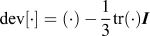 ${\rm dev}[·] = (·) - {1 \over 3}{\rm tr}(·){\bi I}$ is the deviator in the spatial configuration of the indicated argument. The internal variable Q is determined from the following linear rate equation of evolution:
 $$\dot {\bi Q} + {1 \over {t_0 }}{\bi Q} = {{1 - {\rm{\gamma }}} \over {t_0 }}{\rm DEV}\left[ {{{\partial {{\overline \Psi }}^{\,0} (\bar {\bi E})} \over {\partial \bar {\bi E}}}} \right],\,{\bi Q}\left| {_{\rm t = 0} } \right. = 0\quad,$$
where γ is a given parameter and t 0 is the characteristic relaxation time of the material. Equations (7) and (8) give the Kirchhoff stress in the following formReference Simo26:
 $${\rm{\bolditau }} = {\bi FSF}^{\rm T} = Jp{\bi I} + {\rm dev}[\bar {\bi F}{\bi H}\bar {\bi F}^{\rm T} ]\quad,$$
where
 $${\bi H} = \int\limits_0^t {\left( {{\rm{\gamma }} + (1 - {\rm{\gamma }})e^{( - (t - s)/t_0 )} } \right)} {d \over {ds}}\left[ {{{\partial {{\overline \Psi }}^{\,0} (\bar {\bi E})} \over {\partial \bar {\bi E}}}} \right]ds\quad\!,$$
Here, 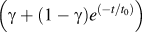 $\left( {{\rm{\gamma }} + (1 - {\rm{\gamma }})e^{( - t/t_0 )} } \right)$ is the viscoelastic kernel function, representing the relaxation behavior of the material. For more general cases, this kernel function can be defined as Prony series with several relaxation times, e.g.,
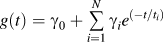 $g(t) = {\rm{\gamma }}_0 + \mathop\sum\limits_{i = 1}^N {{\rm{\gamma }}_i } e^{( - t/t_i )} $. The initial elastic stored energy function Ψ0 could have many choices as well. For example, when the strain energy function for the classical neo-Hookean model is adopted,
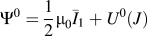 ${\rm{\Psi }}^0 = {1 \over 2}{\rm{\mu }}_0 \bar I_1 + U^0 (J)$, where μ0 is the initial shear modulus and
 $\bar I_1 $is the first deviatoric strain invariant.
ABAQUS24 amends the above model by taking into account the viscous volumetric response and gives the following set of equations in the spatial configuration for the Kirchhoff stress:
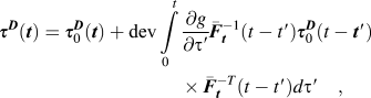 $${\rm{\bolditau }}^{\bi D} ({\bi t}) = {\rm{\bolditau }}_{0}^{\bi D} ({\bi t}) + {\rm dev}\int\limits_0^t \,{{{\partial g} \over {\partial {\rm{\tau \prime}}}}} \bar {\bi F}_{\bi t} ^{ - 1} (t - t\prime){\rm{\bolditau }}_{0}^{\bi D} (t - {\bi t\prime})\bar {\bi F}_{\bi t} ^{ - T} (t - t\prime)d{\rm{\tau \prime}}\quad,$$
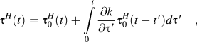 $${\rm{\boldtau }}^H (t) = {\rm{\boldtau }}_0^H (t) + \int\limits_0^t {{{\partial k} \over {\partial {\rm{\tau \prime}}}}{\rm{\boldtau }}_0^H (t - t\prime)d{\rm{\tau \prime}}} \quad,$$
where τD and τH are the deviatoric and the hydrostatic parts of the Kirchhoff stress. 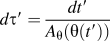 $d{\rm{\tau \prime}} = {{dt\prime} \over {A_{\rm{\theta }} ({\rm{\theta }}(t\prime))}}$, where θ is the temperature and A θ the shift function.24
 $\bar {\bi F}_t (t - t\prime)$ represents the isochoric part of the deformation gradient of the state at t − t′ relative to the state at t. g and k are the shear and bulk viscoelastic kernel functions, respectively. In this paper, we focus on the case where the Poisson’s ratio is time independent, and hence, g = k.
 ${\rm{\bolditau }}_{0}^{\bi D} $ and
 ${\rm{\bolditau }}_{0}^{\bi H} $ are determined from the initial elastic stored energy function Ψ0. In this study, Ψ0 corresponding to the Arruda–Boyce hyperelastic modelReference Arruda and Boyce32 is used, which is given by:
 $$\eqalign{ {\rm{\Psi }}^0 & = {\rm{\mu }}\left\{ {{1 \over 2}(\bar I_1 - 3) + {1 \over {20{\rm{\lambda }}_m^2 }}(\bar I_1^2 - 9) + {{11} \over {1050{\rm{\lambda }}_m^4 }}(\bar I_1^3 - 27) \cr + {{19} \over {7000{\rm{\lambda }}_m^6 }}(\bar I_1^4 - 81) + {{519} \over {673,75{\rm{0}}\lambda _m^8 }}(\bar I_1^5 - 243)} \right\} \cr & + {1 \over D}\left( {{{J_{{\rm{el}}}^2 - 1} \over 2} - \ln J_{{\rm{el}}} } \right)\quad, \cr} $$
where μ, λm, and D are material parameters and λm is the locking stretch at which upturn of the stress–strain curve would rise significantly. J el is the elastic volume ratio. The initial shear modulus μ0 is related to the shear modulus μ by:
 $${\rm{\mu }}_0 = {\rm{\mu }}\left( {1 + {3 \over {5{\rm{\lambda }}_m^2 }} + {{99} \over {175{\rm{\lambda }}_m^4 }} + {{513} \over {875{\rm{\lambda }}_m^6 }} + {{42,039} \over {67,375{\rm{\lambda }}_m^8 }}} \right)\quad.$$
The initial bulk modulus K 0 is related to D with the expression  $K_0 = {2 \over D}$, where D is zero for incompressible materials. A typical value of λm is in the range of 3–7 for common rubbers and it is usually in the range of 1–2 for some soft elastomers and many biological soft tissues.
The viscoelastic kernel function g can be defined in the following form:
 $$g = 1 - {\rm{\chi }}(t)\quad,$$
where  ${\rm{\chi }}(t)$ is a function with
 ${\rm{\chi }}(0) = 0$ and
 $0\, \le\, {\rm{\chi }}(t) \,\lt\, 1$. Prony series is usually used to define
 ${\rm{\chi }}(t)$as:
 $${\rm{\chi }}(t) = \mathop\sum\limits_{{\rm{\alpha }} = 1}^M {g_{\rm{\alpha }} [1 - \exp ( - t/{\rm{\tau }}_{\rm{\alpha }} )]} \quad,$$
where g α is a positive real number defining the extent of the relaxation of the material, τα represents the characteristic relaxation time, and M is an integer.
B. Finite element analysis
The scaling relation in Eq. (1) can be generalized to the indentation of nonlinear viscoelastic materials with the constitutive model described in Sec. II. A as:
 $$g = \bar P\quad .$$
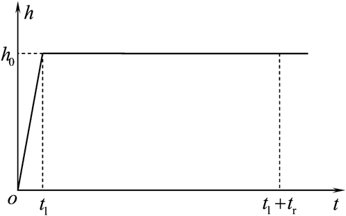
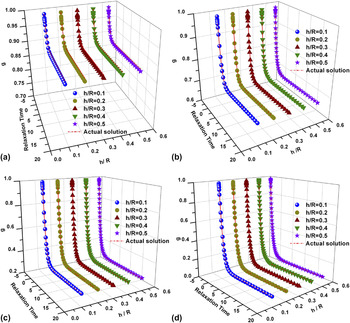
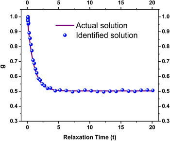
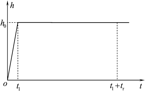
An analytical proof of Eq. (16) is difficult because of the highly nonlinear feature of the problem. So in this section, a series of finite element simulations are performed to examine the applicability of Eq. (16). The displacement-controlled loading procedure adopted in the numerical experiments is given by Fig. 1. In the analysis, the time t 1 at which the indenter reaches the maximum depth is taken to be smaller than 10% of the minimum characteristic relaxation time, and the relaxation time t r is 10 times the maximum characteristic relaxation time of the material. We first investigate an example of a spherical indenter indenting into a soft layer bonded to a rigid substrate (Fig. 2). A total of 200 cases have been simulated by considering different indentation depths and a wide range of material properties. The ratios of the indentation depth to the thickness of the soft layer vary from 0.1 to 0.5 and λm changes from 1 to 10. First-order Prony series is used to describe the viscoelastic kernel function, g(t), and its value at the time of t = ∞, g(t = ∞), is in the range of 0.1–0.9. Figure 3 compares the identified viscoelastic kernel functions with the actual solutions. Our simulations show that the value of λm has no effect on the identified solution; therefore, λm = 1 is taken for illustration. It can be found from Fig. 3 that for different extents of relaxation, the viscoelastic kernel functions identified from Eq. (16) and the indentation relaxation loads at different indentation depths match the actual solutions remarkably well. Since the viscoelastic kernel function scales with the normalized relaxation load according to Eq. (16), the condition numberReference Cao and Lu33 for the present problem is 1. This indicates that the error level in the identified solution is basically the same as that in the input data as illustrated in Fig. 4.
Loading procedure used in the simulation of indentation relaxation tests.
A spherical indenter indenting into a soft layer bonded to a rigid substrate.

Comparison of the viscoelastic kernel function identified by using Eq. (16) with the actual solutions, λm = 1. (a) g(∞) = 0.9; (b) g(∞) = 0.7; (c) g(∞) = 0.3; and (d) g(∞) = 0.1.

Comparison of the viscoelastic kernel function identified by using Eq. (16) with the actual solutions; 3% random error was introduced to the input data to illustrate the sensitivity of the identified solution to data noise.

We further explore two examples of practical interest. For each example below, we investigate three kinds of nonlinear viscoelastic materials with different viscoelastic kernel functions, referred to as NVM1, NVM2, and PDMS, respectively, as listed in Table I. The material parameters of PDMS are obtained from tensile tests, as described in detail below.
Material parameters of three representative materials used in the computational study in Sec. III.

Here, 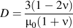 $D = {{3(1 - 2\nu )} \over {{\rm{\mu }}_0 (1 + \nu )}}$.
1. Conical indentation of a substrate with irregular surface profile
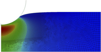
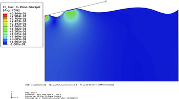
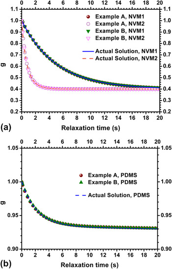
First, we consider the conical indentation of a nonlinear viscoelastic substrate. This example dedicates to verify the applicability of Eq. (16) to the circumstances under which the indented solid has irregular geometry. A total of 12,272 four-node axisymmetric elements are used to model the indented solid. The maximum indentation depth at which the relaxation starts is h 0 = 2 μm, and the corresponding deformed mesh is presented in Fig. 5. The indentation-induced maximum principal logarithmic strain is around 33%. We explore the effects of the locking stretch and the compressibility of the indented material by investigating different values of λm and D in Eq. (13). When D = 0, the material is incompressible, and in the simulations, we use the hybrid element (CPE8H) in ABAQUS instead of the reduced integration element with hourglass control. Using the indentation responses given by finite element computations and Eq. (16), the viscoelastic kernel function g is determined. The results are given by the circle points in Fig. 6, which find a good agreement with the actual solutions (lines).
Contours of the maximum in-plane principal strain for the conical indenter indenting into a solid with irregular surface profile.

Comparison of the viscoelastic kernel function identified by using Eq. (16) with the actual solutions: (a) the results for NVM1 and NVM2 and (b) the results for PDMS.

2. Flat punch indentation of a soft layer bonded to a rigid substrate
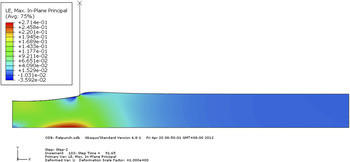
Then, we consider a flat punch indenter indenting into a viscoelastic soft layer bonded to a rigid substrate. This example aims at examining the applicability of Eq. (16) to the cases where the indenter tip has defects and the effects of rigid substrate come into play as well. A total of 10,001 four-node axisymmetric elements are used. The deformation of the indented solid and the contour of the maximum principal logarithmic strain at the maximum indentation depth of 1.5 μm are shown in Fig. 7. Based on the load time relation given by finite element simulations, the viscoelastic kernel function of the indented solid is identified using Eq. (16) and given by the triangle points in Fig. 6. The consistency between the identified results and the actual solutions indicates that Eq. (16) is applicable to this kind of problems.
A flat punch indenter with tip defects indenting into a soft layer.

III. EXPERIMENTS
A. Materials
The material used in the experiments is PDMS. It was prepared by mixing a degassed elastomer base and a cross-linker in a ratio of 10:1 w/w. The prepolymerized mixture was filled in a mold and cured at 60 °C for 8 h. When the PDMS had become a solid state, it was taken out to prepare the specimens.
B. Tensile tests
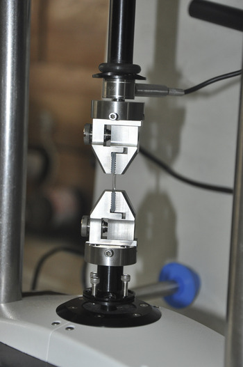
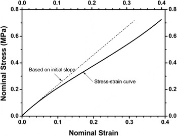
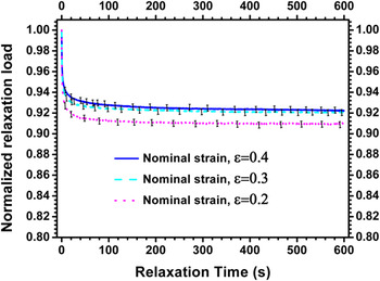
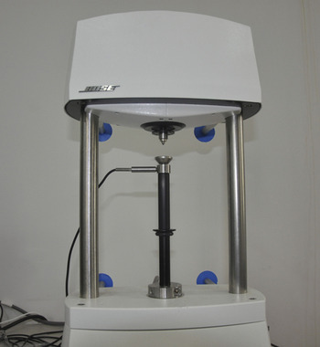
Tensile relaxation tests are performed to determine the viscoelastic kernel functions of the materials, and the results are compared with those identified from indentation tests. The ElectroForce® 3100 test instrument (Bose, Eden Prairie, MN; Fig. 8) is used for the measurements. The specimens have a width of 5 mm, a thickness of 1.8 mm, and a gauge length of 11 mm. Displacement-controlled loading procedure is applied, and the measurements conducted at ambient temperature (23 °C) and the humidity is about 50%. The specimen is first stretched to a given stretch ratio, and then, the tensile relaxation test is performed by keeping this stretching ratio to be constant. The time at which the specimen is stretched to the given stretch ratio is taken as 1 s, which is much shorter than the characteristic relaxation time. A number of different stretch ratios are adopted in the experiments to examine the extent to which the relaxation behavior of the material depends on the deformation. Figure 9 represents a typical tensile curve with the maximum nominal strain up to 40%. It can be found that the tensile curve exhibits nonlinearity when the tensile strain is beyond 20%, which is basically consistent with result reported in the literature (e.g., Fig. 2 in Ref. Reference Zang, Zhao, Cao and Hutchinson34). Figure 10 shows an example for the variation of the relaxation load with time.
Tensile test of PDMS strip performed using the ElectroForce® 3100 test instrument.

Tensile curve of PDMS (1:10), when the nominal strain is beyond 20%, pronounced nonlinearity occurs.

Variation of the relaxation load normalized by the load at the starting point of the tensile relaxation test with time for three different stretch ratios.

C. Indentation tests
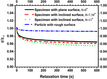
In the measurements, we use the ElectroForce® 3100 test instrument with a spherical indenter of 2.5 mm in radius (Fig. 11). The machine can reach a maximum load of 22 N. The displacement resolution is 1 μm and the load resolution is 0.5 mN. The measurements are performed at room temperature. The displacement-controlled loading procedure shown in Fig. 1 is adopted. Different loading rates are adopted. The results show that when the loading time at which the indenter reaches the maximum indentation depth is smaller than 1 s, the loading curve basically does not depend on the loading rate. Our computational results have demonstrated that the geometry of the indented solid has no effect on the relation given by Eq. (16). This issue has been further examined in our experiments by investigating two critical cases. In the first example, the indentation tests are performed on the specimens with different inclined surface. In the second case, the specimen is a particle with rough surface. For each specimen, at least, five measurements are conducted. The ratio of the indentation depth to the indenter radius is taken as 0.8. The variation of the indentation load with time is recorded and used to determine the viscoelastic kernel functions of the indented material.
Indentation tests performed using the ElectroForce® 3100 test instrument.

D. Results and analysis
To analyze the tensile relaxation test, we need the correlation between the relaxation load and the viscoelastic kernel function involved in the finite strain viscoelastic model in Sec. II. Referring to Findley et al.,Reference Findley, Lai and Onaran35 the derivation of such a relation is given in Appendix. Using Eq. (A11) in Appendix and the tensile loads in the relaxation tests, the viscoelastic kernel function of the material is obtained and plotted in Fig. 12. The errors as illustrated by the error bar are mainly attributed to the difference in the stretch amount in the tensile relaxation tests.
Viscoelastic kernel functions identified using tensile loads and Eq. (A11). The errors (shown as the error bar in the figure) are mainly attributed to the difference in the stretch ratios.

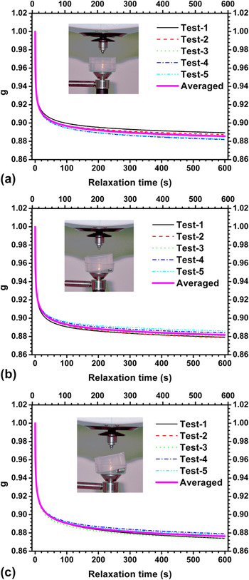
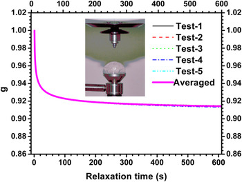
Using Eq. (16), the viscoelastic kernel function g of the material is evaluated from the indentation load–time curves, and the results are depicted in Figs. 13 and 14. Figure 15 shows the relative difference between the indentation results and the tensile results. It can be drawn from Figs. 13 and 14 that indeed, the effects of the geometry of the indented solid on the determination of the viscoelastic kernel function using Eq. (16) are negligible, which is consistent with the computational results. Figure 15 indicates that the viscoelastic kernel function determined using indentation relaxation tests and Eq. (16) matches the result given by tensile relaxation tests well (the relative difference is smaller than 5%). Therefore, Eq. (16) may serve as a fundamental relation to extract the viscoelastic kernel function of nonlinear viscoelastic materials from the responses of indentation relaxation tests. It is of interest to note that Eqs. (16) and (A11) are in the same form though tension and indentation are two fundamentally different types of loading.
Viscoelastic kernel functions identified from indentation relaxation tests and Eq. (16) for the specimens with inclined surfaces: (a) inclined angle θ = 0° ; (b) θ = 7.35° ; and (c) θ = 11° .

Viscoelastic kernel functions identified from indentation relaxation tests and Eq. (16) for the indentation of the particle with rough surface.

Relative difference between the viscoelastic kernel functions given by tensile tests and those given by indentation tests.

IV. CONCLUDING REMARKS
We have explored the indentation of nonlinear viscoelastic materials with focus on the determination of the viscoelastic kernel function, which represents the relaxation behavior of the material. Our finite element simulations based on a typical finite strain viscoelastic model illustrate that the viscoelastic kernel function scales with the normalized indentation relaxation load, i.e.,  $g = \overline P $. Similar to the indentation of linear viscoelastic solids, this relation is independent of the indenter as well as the profile of the indented solid. Therefore, it should be especially useful in the case where the indenter has tip defects or the indented solid has irregular geometry. Experiments have been conducted on PDMS to confirm our computational results and validate the applicability of the relation in practical measurements.
It is emphasized that the present study focuses on the finite strain viscoelastic model with the viscous response characterized by a linear rate constitutive equation, which has been widely used in the literature to characterize the nonlinear viscoelastic solids whose relaxation behavior is basically independent of the deformation. However, some biological soft tissues exhibit strong deformation-dependent relaxation behavior, especially in the case of large deformation.Reference Duenwald, Vanderby and Lakes36 In this case, the deformation behavior cannot be well captured by the single integral hereditary modelReference Ciambella, Paolone and Vidoli37 involved here. Instead, such fully nonlinear models as developed by Reese and GovindjeeReference Reese and Govindjee29 should be used, for which the correlation between the indentation responses and the material properties has not been established and deserves further effort.
ACKNOWLEDGMENTS
Supports from the National Natural Science Foundation of China (Grant Nos. 10972112 and 11210401062), Tsinghua University (Grant Nos. 2012Z02103 and 20121087991), and 973 Program of MOST (Grant No. 2010CB631005) are gratefully acknowledged.
APPENDIX
In the uniaxial tension test of a homogeneous solid, the motion is described by:
 $$x_1 = {\rm{\lambda }}(t)X_1 ,x_2 = J^{1/2} {\rm{\lambda }}(t)^{ - 1/2} X_2 ,x_3 = J^{1/2} {\rm{\lambda }}(t)^{ - 1/2} X_3 \quad,$$
where xi (i = 1, 2, 3) and XI (I = 1, 2, 3) represent the coordinates in the spatial and reference configuration, respectively, λ(t) is the stretch ratio in the direction of the uniaxial tension, and J is the determinant of the deformation gradient. The deformation gradient has the diagonal form:
 $${\bi F}(t) = {\rm{Diag}}\Big[{\rm{\lambda }}(t),J^{1/2} {\rm{\lambda }}(t)^{ - 1/2} ,J^{1/2} {\rm{\lambda }}(t)^{ - 1/2} \Big]\quad.$$
We consider a tensile relaxation test, where the stretch ratio is described via a Heaviside step function:
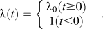 $${\rm{\lambda }}(t) = \left\{ {\matrix{ {{\rm{\lambda }}_0 (t \ge 0)} \cr {1(t \lt 0)} \cr } } \right.\quad.$$
The instantaneous Kirchhoff stress τ0(t) is the function of the material parameters, the stretch ratio, and the determinant of the deformation gradient J. When t ≥ 0, the stretch ratio λ(t) in a tensile relaxation test and J are constant, and hence, the Kirchhoff stress τ0(t) also does not change, which is written as τ0 here. In this case, it is obvious that  $\bar {\rm F}_t (t - t\prime)$ is a second-order unit tensor. Therefore, from Eq. (9), we have:
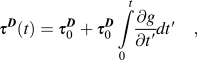 $${\rm{\bolditau }}^{\bi D} ({t}) = {\rm{\bolditau }}_{0}^{\bi D} + {\rm{\bolditau }}_{0}^{\bi D} \int\limits_0^t {{{\partial g} \over {\partial t\prime}}} dt\prime\quad,$$
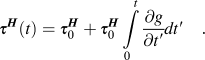 $${\rm{\bolditau }}^{\bi H} ({ t}) = {\rm{\bolditau }}_{0}^{\bi H} + {\rm{\bolditau }}_{ 0}^{\bi H} \int\limits_0^t {{{\partial g} \over {\partial t\prime}}} dt\prime\quad.$$
Further, the Kirchhoff stress τ(t) is:
 $${\rm{\bolditau }}({\bi t}) = {\rm{\bolditau }}^{\bi D} ({ t}) + {\rm{\bolditau }}^{\bi H} ({t}) = {\rm{\bolditau }}_{0} \left( {1 + \int\limits_0^t {{{\partial g} \over {\partial t\prime}}} dt\prime} \right)\quad.$$
Recall that g(0) = 1, Eq. (A6) can be further reduced to:
 $${\rm{\bolditau }}({\bi t}) = {\rm{\bolditau }}_{0} g(t)\quad.$$
In the current configuration, the Cauchy stress can be expressed as:
 $${\rm{\boldisigma }}({\bi t}) = J{\rm{\bolditau }}({\bi t})\quad.$$
Then, the uniaxial tensile load may be written as:
 $$P_u (t) = {\rm{\sigma }}_{11} (t)A(0)/{\rm{\lambda }}_0 \quad,$$
where A(0) represents the area of the initial cross section. σ 11 is the Cauchy stress in the tensile direction. Equations (A7)−(A9) give:
 $$P_u (t) = J{\rm{\tau }}_{011} g(t)A(0)/{\rm{\lambda }}_0 \quad,$$
where τ011 is the instantaneous Kirchhoff stress in the tensile direction. It is of notice that g(0) = 1 and  $P_u (0) = J{\rm{\tau }}_{011} A(0)/{\rm{\lambda }}_0 $, from Eq. (A10), we get the following correlation between the viscoelastic kernel function g(t) and the relaxation load:
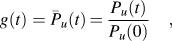 $$g(t) = \bar P_u (t){\rm{ \,=\, }}{{P_u (t)} \over {P_u (0)}}\quad,$$
where Pu(0) is the tension load at the starting point of relaxation.