3.1 Asymptotic analysis

The inviscid linear stability of Batchelor vortices is analysed in cylindrical polar coordinates. Each flow variable is assumed to consist of its mean part ($\!~^{\overline{\quad }}$) and a small amplitude disturbance ($\widetilde{\quad }$). These flow variables are written as

(3.1)$$\begin{eqnarray}\left\{\begin{array}{@{}c@{}}\unicode[STIX]{x1D70C}(r,\unicode[STIX]{x1D703},x,t)\\ u_{r}(r,\unicode[STIX]{x1D703},x,t)\\ u_{\unicode[STIX]{x1D703}}(r,\unicode[STIX]{x1D703},x,t)\\ u_{x}(r,\unicode[STIX]{x1D703},x,t)\\ p(r,\unicode[STIX]{x1D703},x,t)\end{array}\right\}=\left\{\begin{array}{@{}c@{}}\overline{\unicode[STIX]{x1D70C}}(r)\\ \overline{u}_{r}(r)\\ \overline{u}_{\unicode[STIX]{x1D703}}(r)\\ \overline{u}_{x}(r)\\ \overline{p}(r)\end{array}\right\}+\left\{\begin{array}{@{}c@{}}\widetilde{\unicode[STIX]{x1D70C}}(r,\unicode[STIX]{x1D703},x,t)\\ \widetilde{u}_{r}(r,\unicode[STIX]{x1D703},x,t)\\ \widetilde{u}_{\unicode[STIX]{x1D703}}(r,\unicode[STIX]{x1D703},x,t)\\ \widetilde{u}_{x}(r,\unicode[STIX]{x1D703},x,t)\\ \widetilde{p}(r,\unicode[STIX]{x1D703},x,t)\end{array}\right\}.\end{eqnarray}$$

In terms of the normal modes, the linear disturbances are expressed as

(3.2)$$\begin{eqnarray}\{\widetilde{\unicode[STIX]{x1D70C}},\widetilde{u}_{r},\widetilde{u}_{\unicode[STIX]{x1D703}},\widetilde{u}_{x},\widetilde{p}\}=\{R(r),U(r),V(r),W(r),P(r)\}\exp [\boldsymbol{i}(\unicode[STIX]{x1D6FC}x+m\unicode[STIX]{x1D703}-\unicode[STIX]{x1D714}t)],\end{eqnarray}$$

where $m$ is the azimuthal wavenumber (integer), $\unicode[STIX]{x1D6FC}$ is the axial wavenumber (real) and $\unicode[STIX]{x1D714}=\unicode[STIX]{x1D714}_{r}+\boldsymbol{i}\,\unicode[STIX]{x1D714}_{i}$ (complex), where $\unicode[STIX]{x1D714}_{r}$ is the angular frequency and $\unicode[STIX]{x1D714}_{i}$ is the temporal growth rate. The inviscid linearized disturbance equations are written as

(3.3a,b)$$\begin{eqnarray}\frac{\text{d}P}{\text{d}r}=A(r)P+B(r)U,\quad \frac{\text{d}U}{\text{d}r}=C(r)P+D(r)U,\end{eqnarray}$$

(3.4)$$\begin{eqnarray}\left.\begin{array}{@{}c@{}}A(r)=\displaystyle {\displaystyle \frac{{\overline{u}_{\unicode[STIX]{x1D703}}}^{2}}{r\overline{c}^{2}}}-\displaystyle {\displaystyle \frac{2m\overline{u}_{\unicode[STIX]{x1D703}}}{r^{2}\overline{\unicode[STIX]{x1D719}}}},\quad B(r)=\displaystyle {\displaystyle \frac{\boldsymbol{i}\overline{\unicode[STIX]{x1D70C}}}{\overline{\unicode[STIX]{x1D719}}}}\left(N^{2}+\displaystyle {\displaystyle \frac{2\overline{u}_{\unicode[STIX]{x1D703}}\overline{\unicode[STIX]{x1D714}}_{x}}{r}}-\overline{\unicode[STIX]{x1D719}}^{2}\right),\\ C(r)=\displaystyle {\displaystyle \frac{\boldsymbol{i}}{\overline{\unicode[STIX]{x1D70C}}\overline{\unicode[STIX]{x1D719}}}}\left(\unicode[STIX]{x1D6FC}^{2}+\displaystyle {\displaystyle \frac{m^{2}}{r^{2}}}-\displaystyle {\displaystyle \frac{\overline{\unicode[STIX]{x1D719}}^{2}}{\overline{c}^{2}}}\right),\quad D(r)=\displaystyle {\displaystyle \frac{1}{\overline{\unicode[STIX]{x1D719}}}}\left(\frac{m}{r}\overline{\unicode[STIX]{x1D714}}_{x}-\unicode[STIX]{x1D6FC}\overline{\unicode[STIX]{x1D714}}_{\unicode[STIX]{x1D703}}\right)-\displaystyle {\displaystyle \frac{{\overline{u}_{\unicode[STIX]{x1D703}}}^{2}}{r\overline{c}^{2}}}-\displaystyle {\displaystyle \frac{1}{r}},\!\end{array}\right\}\end{eqnarray}$$

where

(3.5a-d)$$\begin{eqnarray}\overline{\unicode[STIX]{x1D719}}=-\unicode[STIX]{x1D714}+m\frac{\overline{u}_{\unicode[STIX]{x1D703}}}{r}+\unicode[STIX]{x1D6FC}\overline{u}_{x},\quad N^{2}=-\frac{{\overline{u}_{\unicode[STIX]{x1D703}}}^{2}}{\unicode[STIX]{x1D6FE}r}\frac{\text{d}\overline{s}}{\text{d}r},\quad \overline{\unicode[STIX]{x1D714}}_{x}=\frac{\text{d}\overline{u}_{\unicode[STIX]{x1D703}}}{\text{d}r}+\frac{\overline{u}_{\unicode[STIX]{x1D703}}}{r},\quad \overline{\unicode[STIX]{x1D714}}_{\unicode[STIX]{x1D703}}=-\frac{\text{d}\overline{u}_{x}}{\text{d}r}.\end{eqnarray}$$

Here, $\overline{\unicode[STIX]{x1D719}}$ is the Doppler frequency and $N$ is the Brunt–Väisälä frequency.

Introducing a small parameter $\unicode[STIX]{x1D700}$ ($0<\unicode[STIX]{x1D700}\ll 1$) to define the rescaled wavenumbers; $\tilde{m}=\unicode[STIX]{x1D700}m$, $\tilde{\unicode[STIX]{x1D6FC}}=\unicode[STIX]{x1D700}\unicode[STIX]{x1D6FC}$ (Leblanc & Le Duc Reference Leblanc and Le Duc2005; Di Pierro & Abid Reference Di Pierro and Abid2010) and obtaining $\unicode[STIX]{x1D714}\simeq \unicode[STIX]{x1D6E5}/\unicode[STIX]{x1D700}+\boldsymbol{i}\unicode[STIX]{x1D712}$ as the asymptotic solution of (3.3) at large wavenumbers ($|m|\gg 1$, $|\unicode[STIX]{x1D6FC}|\gg 1$), we can estimate the temporal growth rate $\unicode[STIX]{x1D712}$ whose modes are part of a continuum spectrum. In compressible swirling flows, Hiejima (Reference Hiejima2015b) determined the squared growth rate $\unicode[STIX]{x1D712}^{2}$ as

(3.6)$$\begin{eqnarray}\displaystyle & \displaystyle \unicode[STIX]{x1D712}^{2}(r)=\unicode[STIX]{x1D712}_{\text{I}}^{2}+\unicode[STIX]{x1D712}_{\text{II}}^{2}+\unicode[STIX]{x1D712}_{\text{III}}^{2}+\unicode[STIX]{x1D712}_{\text{IV}}^{2}, & \displaystyle\end{eqnarray}$$

(3.7)$$\begin{eqnarray}\displaystyle & \displaystyle \unicode[STIX]{x1D712}_{\text{I}}^{2}=-N^{2}, & \displaystyle\end{eqnarray}$$

(3.8)$$\begin{eqnarray}\displaystyle & \displaystyle \unicode[STIX]{x1D712}_{\text{II}}^{2}=\unicode[STIX]{x1D6F6}(r)\frac{r}{\tilde{\unicode[STIX]{x1D6FC}}}\left[\left(\overline{\mathscr{U}}_{i}\times \widetilde{\mathscr{K}}_{i}\;\right)\cdot \overline{\unicode[STIX]{x1D714}}_{x}\right], & \displaystyle\end{eqnarray}$$

(3.9)$$\begin{eqnarray}\displaystyle & \displaystyle \unicode[STIX]{x1D712}_{\text{III}}^{2}=\unicode[STIX]{x1D6F6}(r)\left(\frac{\tilde{m}}{\tilde{\unicode[STIX]{x1D6FC}}}\right)(-\overline{h}), & \displaystyle\end{eqnarray}$$

(3.10)$$\begin{eqnarray}\displaystyle & \displaystyle \unicode[STIX]{x1D712}_{\text{IV}}^{2}=\frac{2\left(\displaystyle \frac{c_{ph}}{\overline{c}}\right)^{2}}{1-\left(\displaystyle \frac{c_{ph}}{\overline{c}}\right)^{2}}\frac{\overline{M}_{\unicode[STIX]{x1D703}}}{r}\overline{c}\overline{\unicode[STIX]{x1D714}}_{x}, & \displaystyle\end{eqnarray}$$

where

(3.11a-c)$$\begin{eqnarray}\unicode[STIX]{x1D6E5}=\tilde{m}\frac{\overline{u}_{\unicode[STIX]{x1D703}}}{r}+\tilde{\unicode[STIX]{x1D6FC}}\overline{u}_{x},\quad \overline{M}_{\unicode[STIX]{x1D703}}=\frac{\overline{u}_{\unicode[STIX]{x1D703}}}{\overline{c}},\quad c_{ph}=\frac{\unicode[STIX]{x1D714}_{r}}{\sqrt{\unicode[STIX]{x1D6FC}^{2}+\left(\displaystyle \frac{m}{r}\right)^{2}}}\simeq \frac{\unicode[STIX]{x1D6E5}}{\sqrt{\tilde{\unicode[STIX]{x1D6FC}}^{2}+\left(\displaystyle \frac{\tilde{m}}{r}\right)^{2}}},\end{eqnarray}$$

(3.12)$$\begin{eqnarray}\unicode[STIX]{x1D6F6}(r)=\frac{2}{\left[r^{2}+\left(\displaystyle \frac{\tilde{m}}{\tilde{\unicode[STIX]{x1D6FC}}}\right)^{2}\right]\left[1-\left(\displaystyle \frac{c_{ph}}{\overline{c}}\right)^{2}\right]}.\end{eqnarray}$$

We define the vector of velocity $\overline{\mathscr{U}}_{i}$ and the vector of disturbance wavenumbers $\widetilde{\mathscr{K}}_{i}$ as

(3.13a,b)$$\begin{eqnarray}\overline{\mathscr{U}}_{i}=\left(\begin{array}{@{}c@{}}\overline{u}_{x}\\ \overline{u}_{\unicode[STIX]{x1D703}}\end{array}\right)\quad \widetilde{\mathscr{K}}_{i}=\left(\begin{array}{@{}c@{}}\tilde{\unicode[STIX]{x1D6FC}}\\ \tilde{m}/r\end{array}\right).\end{eqnarray}$$

The term $\text{II}$ in (3.6) is expressed as the variable depending on the cross product of the two vectors. In addition, the vorticity vector $\overline{\mathscr{W}}_{i}$ is defined as

(3.14)$$\begin{eqnarray}\overline{\mathscr{W}}_{i}=\left(\begin{array}{@{}c@{}}\overline{\unicode[STIX]{x1D714}}_{x}\\ \overline{\unicode[STIX]{x1D714}}_{\unicode[STIX]{x1D703}}\end{array}\right).\end{eqnarray}$$

The term $\text{III}$ in (3.6) includes the helicity density $\overline{h}$, given by

(3.15)$$\begin{eqnarray}\overline{h}=\overline{\mathscr{U}}_{i}\,\overline{\mathscr{W}}_{i}.\end{eqnarray}$$

Moreover, $\unicode[STIX]{x1D714}_{r}\simeq \unicode[STIX]{x1D6E5}/\unicode[STIX]{x1D700}$ denotes the angular frequency and the term $\text{IV}$ in (3.6) is related to $\unicode[STIX]{x1D6E5}$, which can be rewritten as

(3.16)$$\begin{eqnarray}\unicode[STIX]{x1D6E5}=\overline{\mathscr{U}}_{i}\,\overline{\mathscr{K}}_{i}.\end{eqnarray}$$

Furthermore, taking the derivative of $\unicode[STIX]{x1D6E5}$ in (3.11), we derive the relation

(3.17)$$\begin{eqnarray}\unicode[STIX]{x1D6E5}^{\prime }+\frac{2\,\tilde{m}\,\overline{u}_{\unicode[STIX]{x1D703}}}{r^{2}}=\overline{\mathscr{W}}_{i}\times \widetilde{\mathscr{K}}_{i},\end{eqnarray}$$

where the prime denotes differentiation with respect to $r$. Thus, the three vectors influence each other on stability conditions.

The terms in (3.6) describe four types of destabilizing elements in swirling wake flows. Term $\text{I}$ expresses the entropy gradient related to compressibility effects (Hiejima Reference Hiejima2019). Note that when the stagnation temperature is uniform in the thermodynamic profile, $\unicode[STIX]{x1D712}_{\text{I}}^{2}$ can be rewritten as

(3.18)$$\begin{eqnarray}\unicode[STIX]{x1D712}_{\text{I}}^{2}=-\frac{\overline{M}_{\unicode[STIX]{x1D703}}}{r}\left(\overline{\mathscr{U}}_{i}\times \overline{\mathscr{W}}_{i}\right)\!.\end{eqnarray}$$

Here, we have used (2.11), (3.5) and (3.11). Equation (3.18) indicates that when $q$ is large, the vortex becomes stabilised because term $\text{I}$ becomes large and negative. Term $\text{II}$ includes the sources of helical-shear effects that occur in the vortex core, i.e. the spiral instability. Term $\text{III}$ describes the negative helicity density on the swirling wake flows. Defining the angle between $\overline{\mathscr{U}}_{i}$ and $\overline{\mathscr{W}}_{i}$ as $\unicode[STIX]{x1D713}$, the instability caused by this term (the name ‘helicity instability’) exists over $\unicode[STIX]{x03C0}/2<\unicode[STIX]{x1D713}<3/2\unicode[STIX]{x03C0}$ if the angle is a blunt angle. Note that helicity instability is qualified for the case of axial flow with wake. Term $\text{IV}$ includes the phase velocity $c_{ph}$ and the local speed of sound $\overline{c}$, which are related to the acoustic unstable wave, and is very weak in wake-type flows. Evidently, term $\text{I}$ is determined only by the velocity profiles in the base flow, while terms $\text{II}$, $\text{III}$ and $\text{IV}$ are included in the disturbance wavenumbers. The growth rate of the asymptotic analysis is thus obtained from (3.6), but $(\tilde{m}/\tilde{\unicode[STIX]{x1D6FC}})$ is unknown.

Eckhoff & Storesletten (Reference Eckhoff and Storesletten1978) and Leblanc & Le Duc (Reference Leblanc and Le Duc2005) assumed that, for some $r_{0}$ in compressible swirling flows,

(3.19)$$\begin{eqnarray}\unicode[STIX]{x1D6E5}^{\prime }(r_{0})=0.\end{eqnarray}$$

From (3.19), $(\tilde{m}/\tilde{\unicode[STIX]{x1D6FC}})$ is obtained. In compressible cases, the two conditions (3.6) and (3.19) are comparable to those of incompressible homogenous flows found by Leibovich & Stewartson (Reference Leibovich and Stewartson1983). Therefore, $\unicode[STIX]{x1D712}_{0}=\sqrt{\unicode[STIX]{x1D712}^{2}(r_{0})}$ is uniquely determined from the base flows alone.

Although the Lamb–Oseen vortex is always stable, the Batchelor vortex becomes unstable depending on the axial velocity deficit in incompressible flows (Alekseenko et al. Reference Alekseenko, Kuibin and Okulov2007). 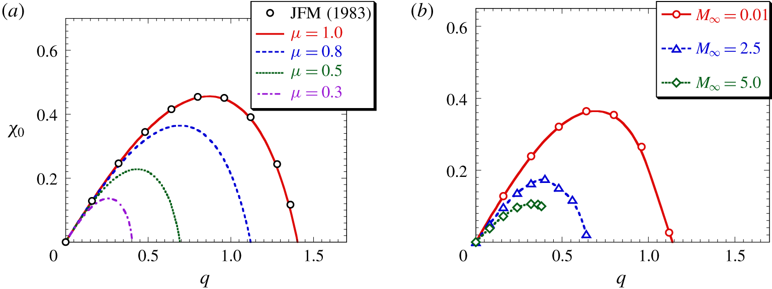To verify the effect of the axial velocity deficit in conventional Batchelor vortices ($D=1.0$ and $M_{\infty }=0.01$), the relations between the growth rate $\unicode[STIX]{x1D712}_{0}$ in (3.6) and the swirl number $q$ at deficit $\unicode[STIX]{x1D707}$ are shown in figure 1(a). When $\unicode[STIX]{x1D707}=1.0$, the maximum $q$ approximated $\sqrt{2}$, consistent with the very strong inviscid mode of the incompressible Batchelor vortex for $q<1.5$ (Heaton & Peake Reference Heaton and Peake2007). The growth rates $\unicode[STIX]{x1D712}_{0}$ were also in good agreement with that of Leibovich & Stewartson (Reference Leibovich and Stewartson1983). Note that the asymptotic growth rate of Billant & Gallaire (Reference Billant and Gallaire2013) is more accurate than that of Leibovich & Stewartson (Reference Leibovich and Stewartson1983) over a wider range of axial wavenumbers in the Batchelor vortex. The growth rate and existence range of the unstable mode decreased with decreasing deficit $\unicode[STIX]{x1D707}$. The $\unicode[STIX]{x1D707}$ exerted a large effect on growth rate, as evidenced by dividing the growth rate $\unicode[STIX]{x1D712}_{0}$ for $\unicode[STIX]{x1D707}=0.3$ by that for $\unicode[STIX]{x1D707}=1.0$. To understand the effect of the Mach number $M_{\infty }$ on the growth rate $\unicode[STIX]{x1D712}_{0}$, we plotted the relations between the growth rate $\unicode[STIX]{x1D712}_{0}$ and the circulation $q$ for three Mach numbers at $\unicode[STIX]{x1D707}=0.8$ (see figure 1b). Both $\unicode[STIX]{x1D712}_{0}$ and $q$ at the maximum growth rate decreased with increasing $M_{\infty }$. For instance, the maximum growth rate was smaller at $M_{\infty }=2.5$ and $\unicode[STIX]{x1D707}=0.8$ than at $M_{\infty }=0.01$ and $\unicode[STIX]{x1D707}=0.8$, and corresponded to that between $\unicode[STIX]{x1D707}=0.3$ and 0.5 at $M_{\infty }=0.01$. In figure 1(b), note the end point of the line at $M_{\infty }=5.0$. This point marks the limit of $q$ because the static pressure at the vortex centre of a compressible flow must be positive.

Figure 1.

Temporal growth rates $\unicode[STIX]{x1D712}_{0}$ in (3.6) as functions of circulation $q$ for $D=1.0$: (a) various $\unicode[STIX]{x1D707}$ at $M_{\infty }=0.01$; ○, the growth rate obtained from the formula given by Leibovich & Stewartson (Reference Leibovich and Stewartson1983); (b) three Mach numbers $M_{\infty }$ at $\unicode[STIX]{x1D707}=0.8$.

Figure 2.

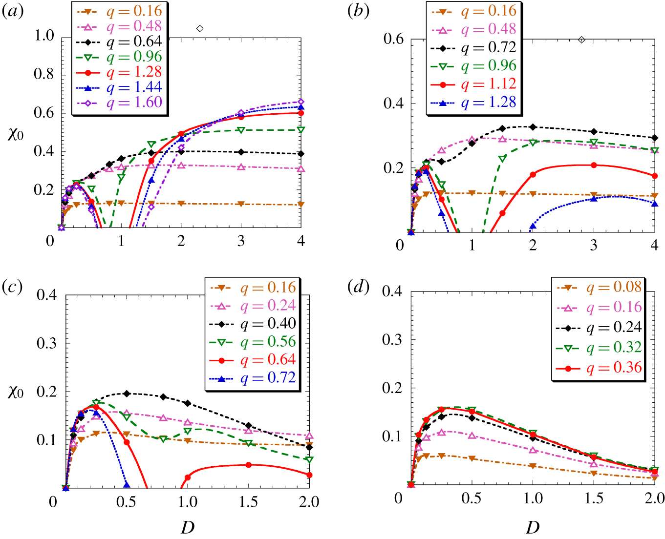
Temporal growth rates $\unicode[STIX]{x1D712}_{0}$ as functions of the parameter $D$ in the asymptotic analysis (3.6) for various $q$ and $\unicode[STIX]{x1D707}=0.8$: (a) $M_{\infty }=0.01$, (b) $M_{\infty }=1.0$, (c) $M_{\infty }=2.5$ and (d) $M_{\infty }=5.0$.

3.2 Helicity instability in the case of axial flow with wake

Figure 2 plots the temporal growth rate $\unicode[STIX]{x1D712}_{0}$ in (3.6) as a function $D$ for $\unicode[STIX]{x1D707}=0.8$ at $M_{\infty }=0.01$, 1.0, 2.5 and 5.0. Note that when $D=0$, the vortex (2.8) corresponds to the Lamb–Oseen vortex (stable vortex). When $M_{\infty }=0.01$, the effect of $D$ on small $q$ is weak. As $q$ increases, the $\unicode[STIX]{x1D712}_{0}$ divides dichotomously. Note that the vortex with large $q$ is stable at $D=1.0$, while it becomes unstable with decreasing and increasing $D$. The results are important in that the stability characteristic has not been investigated in a conventional Batchelor vortex. Although the growth rate of the vortex with large $q$ divides between $D<1.0$ and $D>1.0$ even at $M_{\infty }=1.0$, it decreases at $D>1.0$ in contrast to the case of $M_{\infty }=0.01$. When $M_{\infty }=2.5$ and $D=1.0$, the growth rate was very small at $q=0.64$, and was not observed at $q=0.72$, consistent with the results of figure 1(b). Interestingly, when $q$ was large, the growth rate $\unicode[STIX]{x1D712}_{0}$ rose with decreasing $D$ and the vortices become unstable. When $M_{\infty }=5.0$, all $\unicode[STIX]{x1D712}_{0}$–$D$ curves exhibited a similar feature, that is, the maximum growth rate $\unicode[STIX]{x1D712}_{0}$ for each $q$ occurred at small $D$; moreover, the maximum growth rates at $M_{\infty }=2.5$ and 5.0 were quantitatively similar. In previous works (Hiejima Reference Hiejima2014, Reference Hiejima2019), the Mach-number-dependent stabilisation effect was attributed to term $\text{I}$ in the entropy profile. However, the present result suggests that some other factor associated with the small $D$ explains the destabilisation effect. Elucidating this factor would be helpful for defeating the compressible effects.

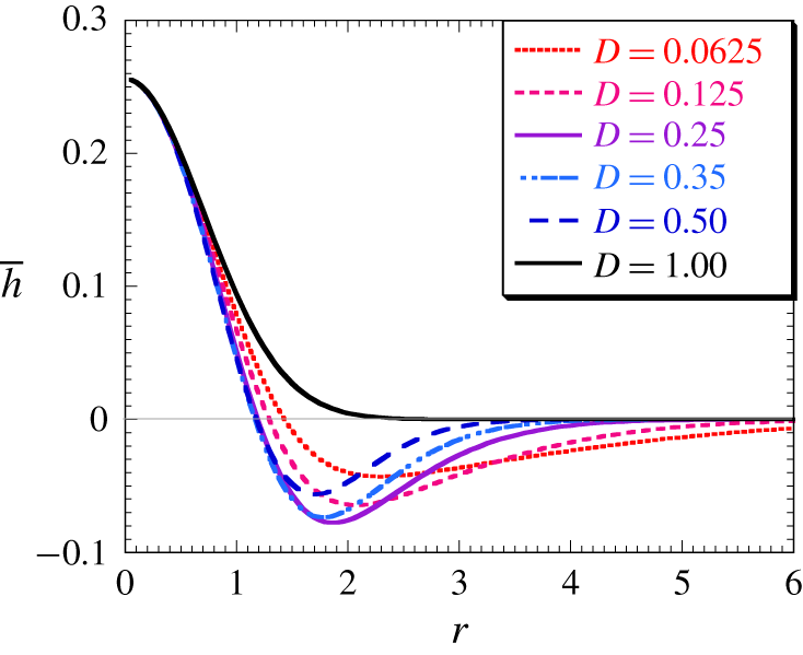
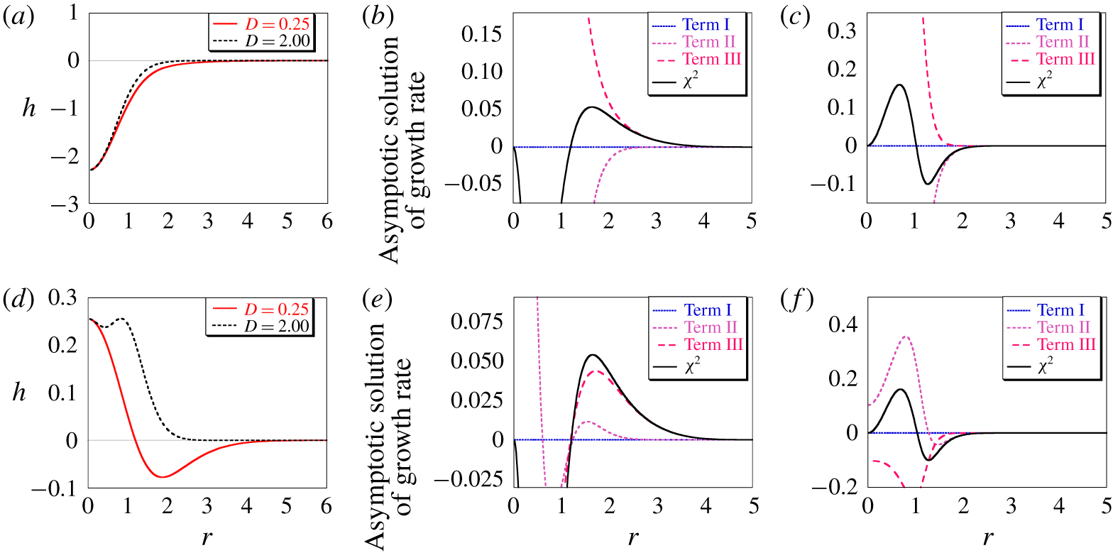
Figure 3 plots the helicity density profiled $\overline{h}$ calculated by (3.15) for various $D$ at $q=0.64$ and $\unicode[STIX]{x1D707}=0.8$. Note that the figure does not depend on the magnitude of $q$ and the helicity density profile varies on the parameter $D$. According to term $\text{III}$ in (3.9), the vortex becomes unstable when the helicity becomes negative (i.e. $\overline{h}<0$) under the axial velocity profiles without reverse flow: $0<\unicode[STIX]{x1D707}\leqslant 1$. Because helicity instability is expressed as term $\text{III}>0$, the degree of helicity instability increases as $D$ reduces. In the case of $D=0.25$, the helicity presented a local minimum at $r=1.85$; this condition is the most effective condition for helicity instability.

Figure 3.

Helicity density profiles $\overline{h}$ for various $D$ at $q=0.64$ and $\unicode[STIX]{x1D707}=0.8$.

Figure 4.

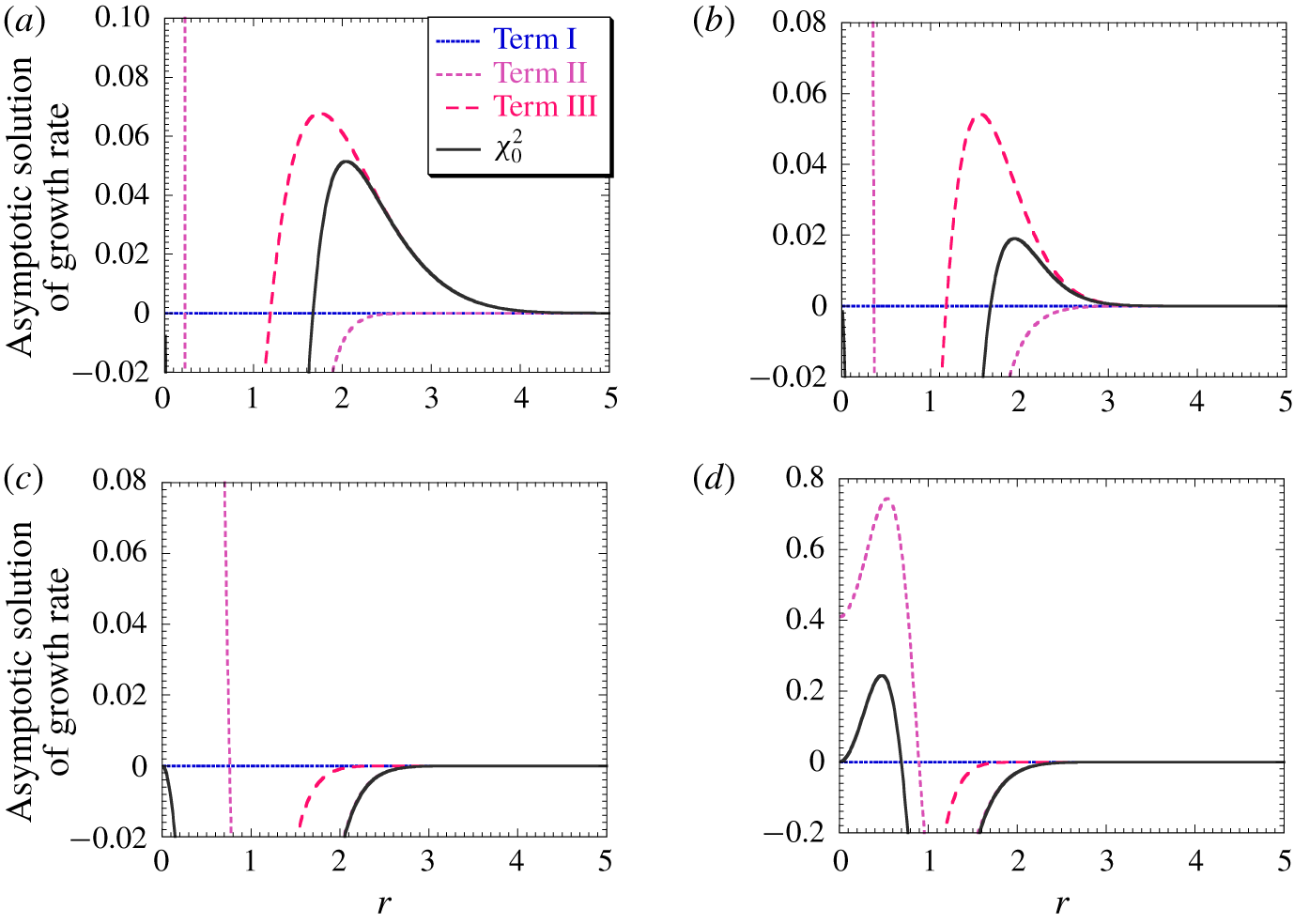
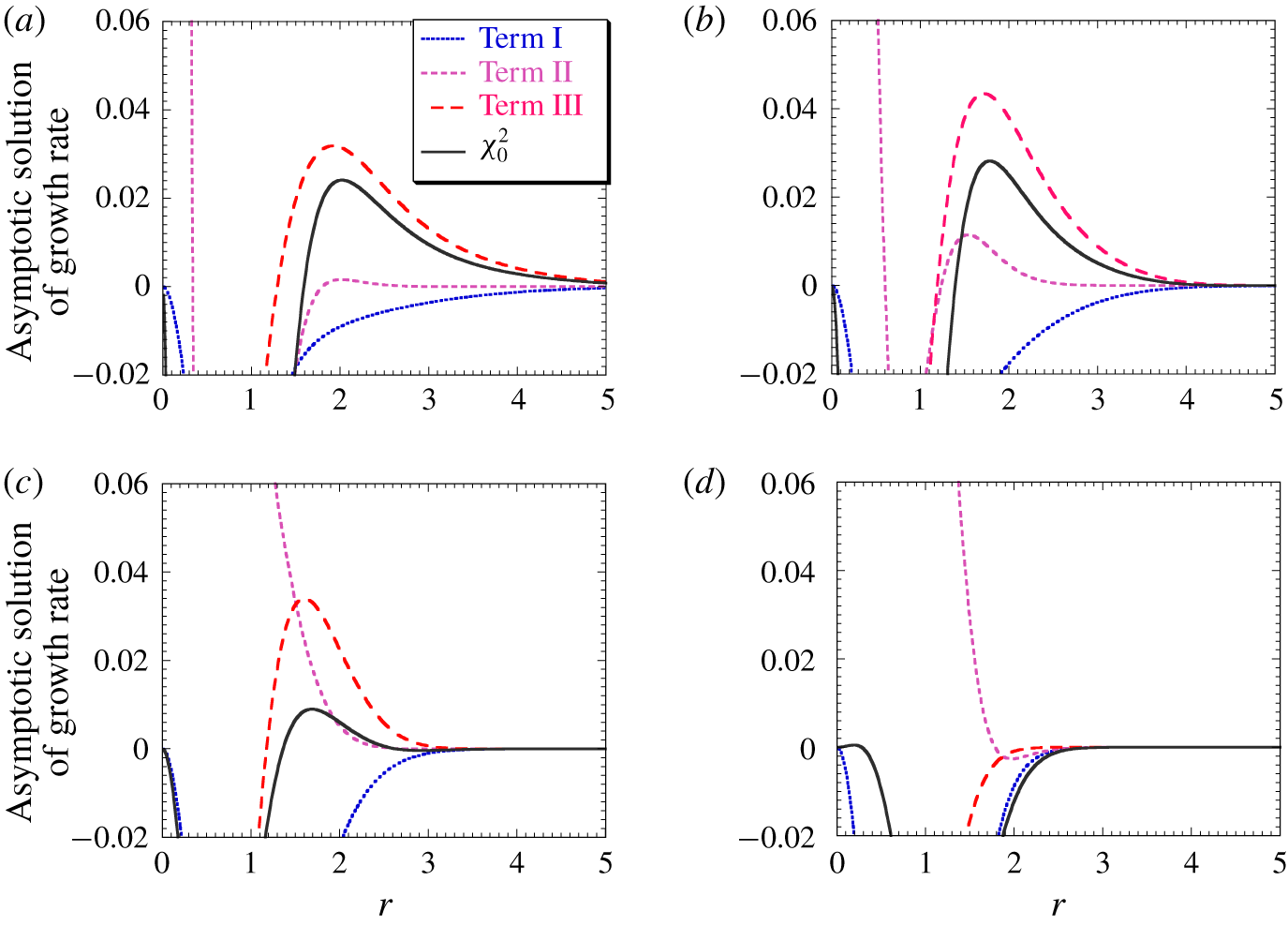
Profiles of squared temporal growth rates $\unicode[STIX]{x1D712}_{0}^{2}$ for each term in (3.6), obtained for a Batchelor vortex with $q=1.28$ and $\unicode[STIX]{x1D707}=0.8$ at $M_{\infty }=0.01$: (a) $D=0.25$, (b) $D=0.50$, (c) $D=1.0$ and (d) $D=2.0$.

Figure 5.

Profiles of squared temporal growth rates $\unicode[STIX]{x1D712}_{0}^{2}$ for each term in (3.6), obtained for a Batchelor vortex with $q=0.64$ and $\unicode[STIX]{x1D707}=0.8$ at $M_{\infty }=2.5$: (a) $D=0.125$, (b) $D=0.25$, (c) $D=0.50$ and (d) $D=1.0$.

Why does a Batchelor vortex with large $q$ stabilise? The mechanism of this phenomenon has not been clarified. As shown in figure 2, the vortices with large $q$ were excitedly destabilised by the parameter $D$, which is related to helicity instability on the condition of $0<\unicode[STIX]{x1D707}\leqslant 1$. Previously, terms $\text{II}$ and $\text{III}$ in (3.6) were considered together, but their individual analyses provide glimpses into new unstable structures in swirling wake flows. In term $\text{II}$, enlarging $q$ also enlarges $-\overline{u}_{\unicode[STIX]{x1D703}}$ and stabilises the vortex because $\unicode[STIX]{x1D712}_{\text{II}}^{2}\propto (\tilde{m}/\tilde{\unicode[STIX]{x1D6FC}})(\overline{u}_{x}/r)-\overline{u}_{\unicode[STIX]{x1D703}}$. In term $\text{III}$, enlarging $D$ stabilises the vortex because $-\overline{h}<0$.

To clarify the dominant instability property, figures 4 and 5 show the distributions of the squared growth rate $\unicode[STIX]{x1D712}_{0}^{2}$ of terms $\text{I}$–$\text{III}$ in (3.6) for various $D$. For an incompressible vortex with $q=1.28$ and $\unicode[STIX]{x1D707}=0.8$, the effect of $D$ on growth rate is shown in figure 4. In all cases, term $\text{I}$ was almost nothing because $M_{\infty }=0.01$. When $D$ was small, the helicity instability that was caused by term $\text{III}$ was strong. When $D=1.0$, the vortex was stable and when $D=2.0$, the strong unstable due to term $\text{II}$ occurred in the vortex core. Note that the feature is close to that of a conventional Batchelor vortex. The effect of term $\text{II}$ decreases as the Mach number increases (see figure 2). In the vicinity of $D=1.0$, the parameter $D$ changes an instability effect from helicity instability (term $\text{III}$) to spiral instability (term $\text{II}$). The results definitely demonstrate the significance of separating terms $\text{II}$ and $\text{III}$ in (3.6). In figure 5 the parameters were fixed as $M_{\infty }=2.5$, $q=0.64$ and $\unicode[STIX]{x1D707}=0.8$ in varying $D$. In all cases, term $\text{I}$ went negative because $M_{\infty }=2.5$. Term $\text{II}$ made a slight contribution around $r=1.5$ only when $D=0.25$. When $D$ was 0.125, 0.25 and 0.50, the helicity effect was large because $\unicode[STIX]{x1D712}_{0}^{2}$ was largely contributed by term $\text{III}$. As seen in (3.18), the stabilisation effect of term $\text{I}$ was high at large $q$, but was largely surpassed by the unstable effect of term $\text{III}$, as shown by $\unicode[STIX]{x1D712}_{0}>0$. As the parameter $D$ decreased, the impacted area spread in the radial direction and the growth rate in all cases was large outside the vortex core. The extension of the instability region beyond the vortex core is likely to be an important feature as will be describe later. When $D=1.0$, term $\text{III}$ almost vanished. In conventional Batchelor vortices ($D=1.0$) with high swirl intensity $q$, the helicity profile participates in the stabilisation. The mechanism is clearly explained by the helicity effect (term $\text{III}$). Therefore, the asymptotic solution distributions in these figures show the features of helicity instability. Further analysis will investigate the instability caused by term $\text{III}$, which relates to the helicity profile. Based on the perspective that the uniform axial velocity component $U_{\infty }^{\ast }$ in (2.2) should not matter in temporal stability, the case of axial flow with jet is described in appendix A.

Figure 6.

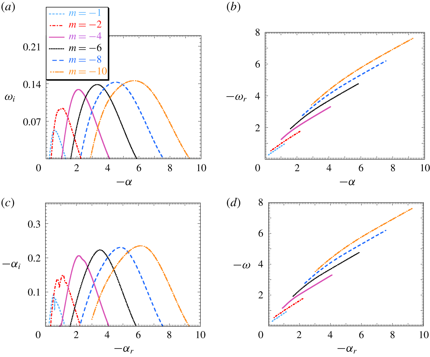
Growth rate (a,c) and frequency (b,d) as functions of axial wavenumber for $q=0.64$, $\unicode[STIX]{x1D707}=0.8$ and $D=0.25$ at $M_{\infty }=2.5$: (a,b) temporal growth and (c,d) spatial growth.

3.3 Temporal and spatial growth rates

Applying linear stability theory, this subsection describes a classical convectively unstable feature of a Batchelor vortex with large $q$. The eigenvalues and eigenfunctions of the inviscid linearized disturbance equations (3.3) were solved by a shooting method. The solution is detailed in the reference (Hiejima Reference Hiejima2013). Increasing the parameter $D$ decreased the growth rate and narrowed the band (data not shown). All modes of $D=1.0$ were stable owing to their small growth rates in the stability analysis. Based on the results of figure 5, the helicity effects were investigated at $D=0.25$, $M_{\infty }=2.5$, $q=0.64$ and $\unicode[STIX]{x1D707}=0.8$.

First, consider the temporal evolution of the vortex. Figure 6(a,b) plots the growth rate $\unicode[STIX]{x1D714}_{i}$ and frequency $\unicode[STIX]{x1D714}_{r}$ as functions of axial wavenumber $\unicode[STIX]{x1D6FC}$. As the $q$ was relatively large, the modes of the low azimuthal wavenumbers were weak. However, the growth rate increased with increasing $m$ and the band of the unstable mode broadened. Part of the phase velocities $\unicode[STIX]{x1D714}_{r}/\unicode[STIX]{x1D6FC}$ were nearly identical without depending on $m$. Here, it is important to compare the present result with the asymptotic analysis (3.6). The ratio of the maximum growth rates $\unicode[STIX]{x1D714}_{i}/\unicode[STIX]{x1D712}_{0}=0.86$ at $m=-10$ and the $\unicode[STIX]{x1D712}_{0}$ overestimates the growth rate, similar to the results of Hiejima (Reference Hiejima2015b). Note that (3.17) satisfies (3.19) when $q$ is small (spiral instability) or $r_{0}$ is large (helicity instability). The present discrepancy possibly arises through the moderate wavenumber, not be enough as an asymptotic solution of (3.3) at large wavenumbers.

Secondly, consider the spatial evolution of the vortex. Setting $\unicode[STIX]{x1D6FC}=\unicode[STIX]{x1D6FC}_{r}+\boldsymbol{i}\,\unicode[STIX]{x1D6FC}_{i}$ (complex), where $\unicode[STIX]{x1D6FC}_{r}$ is the axial wavenumber, $-\unicode[STIX]{x1D6FC}_{i}$ is the spatial growth rate and $\unicode[STIX]{x1D714}$ is the angular frequency (real) in (3.2); the spatial growth rate was obtained by solving (3.3). Figure 6(c,d) plots the growth rate $-\unicode[STIX]{x1D6FC}_{i}$ and frequency $\unicode[STIX]{x1D714}$ as functions of the axial wavenumber $\unicode[STIX]{x1D6FC}_{r}$. Although the features are similar to those of the temporal cases in figure 6(a,b), the profiles for $m=-1$ and $-2$ differ near the maximum growth rate. At the low wavenumbers, because the growth rates were small, crossing modes might occur in spatial growth.

Figure 7.

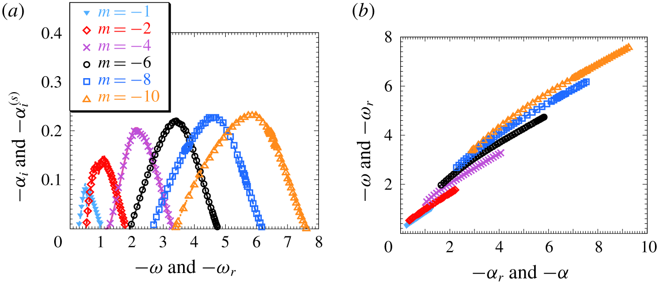
Comparisons of temporal growths and the spatial growth modes for various azimuthal wavenumbers, obtained by the Gaster transformation in (3.20): (a) growth rate versus frequency and (b) frequency versus axial wavenumber.

Thirdly, to better understand the linear unstable property of vortices with helicity instability, we compared their temporal and spatial evolutions. If the local base flows are equal in both growth processes, the group velocity $c_{g}$ of the spatial growth nearly matches that of the temporal growth. The following relation, called the Gaster transformation (Gaster Reference Gaster1968), then holds:

(3.20a-d)$$\begin{eqnarray}\unicode[STIX]{x1D714}^{(s)}=\unicode[STIX]{x1D714}_{r},\quad \unicode[STIX]{x1D6FC}_{r}^{(s)}=\unicode[STIX]{x1D6FC},\quad -\unicode[STIX]{x1D6FC}_{i}^{(s)}=\frac{\unicode[STIX]{x1D714}_{i}}{c_{g}},\quad c_{g}=\frac{\text{d}\unicode[STIX]{x1D714}}{\text{d}\unicode[STIX]{x1D6FC}}.\end{eqnarray}$$

Here the spatial growth property (superscripted by $s$) is transformed from the temporal growth property. Figure 7 plots the growth rate versus frequency and the frequency versus axial wavenumber for various azimuthal wavenumbers. The symbols represent the eigenvalues of the spatial growth transformed from those of temporal growth by (3.20), and the curves are the spatial growth properties. The spatial growth ones were consistent with their transformed values except at some low wavenumbers. This result suggests that the initial spatial growth stage can be understood by obtaining the disturbance features of Batchelor vortices during temporal growth.

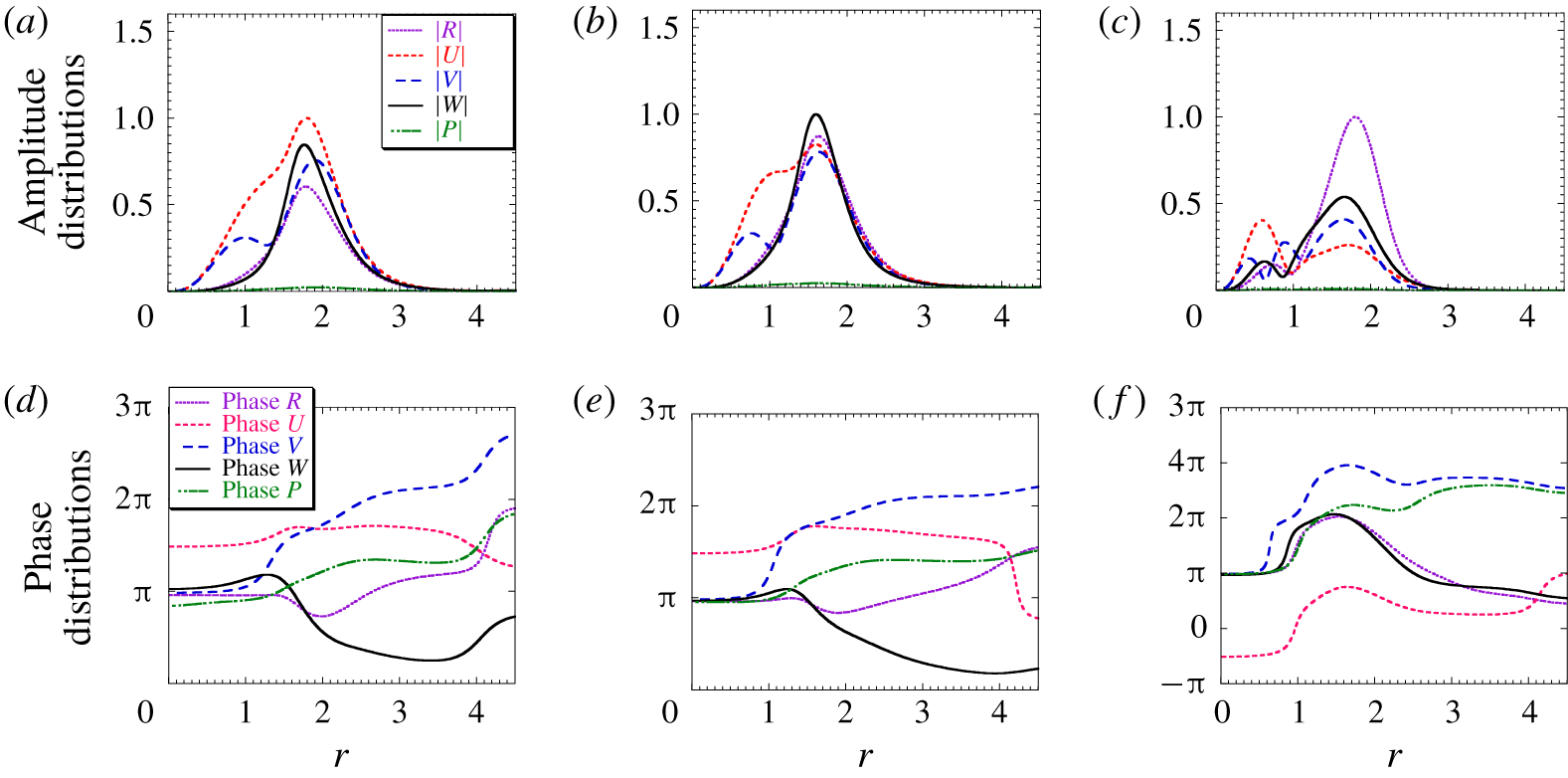
To investigate the disturbance structure associated with helicity instability at $q=0.64$, $\unicode[STIX]{x1D707}=0.8$ and $M_{\infty }=2.5$, the eigenfunction profiles of the disturbance for $m=-4$ are plotted in figure 8. When $D=0.125$ and 0.25, the base flows caused a competition among the velocity disturbances $U$, $V$ and $W$ at the outer edge of the vortex ($r\sim 1.8$). The radial velocity disturbance $U$ was very much larger at $D=0.125$ than in the conventional Batchelor vortex where the amplitude of the axial velocity disturbance is the largest (Delbende & Rossi Reference Delbende and Rossi2005), strongly promoting spreading in the radial direction. When $D=0.50$, although the velocity disturbances also existed at the outer edge of the vortex, the density disturbance was large and repressed the disturbance growth (Hiejima Reference Hiejima2019). Accordingly, terms $\text{I}$ and $\text{III}$ exerted opposing effects on the growth property at $D=0.50$. The phase profiles at $D\leqslant 0.25$ and $D=0.50$ clearly differ in figure 8, and the phase change within $1.5<r<3.5$ depends on the helicity instability effect.

Figure 8.

Eigenfunction profiles of the disturbance for $m=-4$, $q=0.64$ and $\unicode[STIX]{x1D707}=0.8$ at $M_{\infty }=2.5$. Shown are the amplitudes (a–c) and phases (d–f) at (a,d) $D=0.125$, (b,e) $D=0.25$ and (c,f) $D=0.50$.

4.1 Governing equations

From a natural transition perspective, the helicity effect on the spatial evolution of Batchelor vortices subjected to small random noise is investigated using three-dimensional numerical simulations. Note that the simulated velocities and pressure were normalised by using the free stream sonic velocity $c_{\infty }^{\ast }(=\sqrt{\unicode[STIX]{x1D6FE}\,R^{\ast }\,T_{\infty }^{\ast }})$ rather than $U_{\infty }^{\ast }$. The normalised governing equations were the three-dimensional, unsteady, compressible Navier–Stokes equations in general coordinates $\unicode[STIX]{x1D709}_{i}$ ($i=1{-}3$), which are given as

(4.1)$$\begin{eqnarray}\frac{\unicode[STIX]{x2202}}{\unicode[STIX]{x2202}t}\left(\frac{\boldsymbol{Q}}{J}\right)+\frac{\unicode[STIX]{x2202}\boldsymbol{F}_{i}}{\unicode[STIX]{x2202}\unicode[STIX]{x1D709}_{i}}=\frac{\unicode[STIX]{x2202}\boldsymbol{F}_{vi}}{\unicode[STIX]{x2202}\unicode[STIX]{x1D709}_{i}},\end{eqnarray}$$

$$\begin{eqnarray}\boldsymbol{Q}=\left[\begin{array}{@{}c@{}}\unicode[STIX]{x1D70C}\\ \unicode[STIX]{x1D70C}u_{1}\\ \unicode[STIX]{x1D70C}u_{2}\\ \unicode[STIX]{x1D70C}u_{3}\\ e\end{array}\right],\quad \boldsymbol{F}_{i}=\left[\begin{array}{@{}c@{}}\unicode[STIX]{x1D70C}U_{i}\\ \unicode[STIX]{x1D70C}u_{1}U_{i}+p(J^{-1}\unicode[STIX]{x2202}\unicode[STIX]{x1D709}_{i}/\unicode[STIX]{x2202}x_{1})\\ \unicode[STIX]{x1D70C}u_{2}U_{i}+p(J^{-1}\unicode[STIX]{x2202}\unicode[STIX]{x1D709}_{i}/\unicode[STIX]{x2202}x_{2})\\ \unicode[STIX]{x1D70C}u_{3}U_{i}+p(J^{-1}\unicode[STIX]{x2202}\unicode[STIX]{x1D709}_{i}/\unicode[STIX]{x2202}x_{3})\\ (e+p)U_{i}\end{array}\right],\quad \boldsymbol{F}_{vi}=\left[\begin{array}{@{}c@{}}0\\ \unicode[STIX]{x1D70F}_{1k}(J^{-1}\unicode[STIX]{x2202}\unicode[STIX]{x1D709}_{i}/\unicode[STIX]{x2202}x_{k})\\ \unicode[STIX]{x1D70F}_{2k}(J^{-1}\unicode[STIX]{x2202}\unicode[STIX]{x1D709}_{i}/\unicode[STIX]{x2202}x_{k})\\ \unicode[STIX]{x1D70F}_{3k}(J^{-1}\unicode[STIX]{x2202}\unicode[STIX]{x1D709}_{i}/\unicode[STIX]{x2202}x_{k})\\ \unicode[STIX]{x1D6FD}_{k}(J^{-1}\unicode[STIX]{x2202}\unicode[STIX]{x1D709}_{i}/\unicode[STIX]{x2202}x_{k})\\ \end{array}\right],\end{eqnarray}$$

$$\begin{eqnarray}\displaystyle J^{-1} & = & \displaystyle \frac{\unicode[STIX]{x2202}x_{1}}{\unicode[STIX]{x2202}\unicode[STIX]{x1D709}_{1}}\left(\frac{\unicode[STIX]{x2202}x_{2}}{\unicode[STIX]{x2202}\unicode[STIX]{x1D709}_{2}}\frac{\unicode[STIX]{x2202}x_{3}}{\unicode[STIX]{x2202}\unicode[STIX]{x1D709}_{3}}-\frac{\unicode[STIX]{x2202}x_{2}}{\unicode[STIX]{x2202}\unicode[STIX]{x1D709}_{3}}\frac{\unicode[STIX]{x2202}x_{3}}{\unicode[STIX]{x2202}\unicode[STIX]{x1D709}_{2}}\right)+\frac{\unicode[STIX]{x2202}x_{1}}{\unicode[STIX]{x2202}\unicode[STIX]{x1D709}_{2}}\left(\frac{\unicode[STIX]{x2202}x_{2}}{\unicode[STIX]{x2202}\unicode[STIX]{x1D709}_{3}}\frac{\unicode[STIX]{x2202}x_{3}}{\unicode[STIX]{x2202}\unicode[STIX]{x1D709}_{1}}-\frac{\unicode[STIX]{x2202}x_{2}}{\unicode[STIX]{x2202}\unicode[STIX]{x1D709}_{1}}\frac{\unicode[STIX]{x2202}x_{3}}{\unicode[STIX]{x2202}\unicode[STIX]{x1D709}_{3}}\right)\nonumber\\ \displaystyle & & \displaystyle +\,\frac{\unicode[STIX]{x2202}x_{1}}{\unicode[STIX]{x2202}\unicode[STIX]{x1D709}_{3}}\left(\frac{\unicode[STIX]{x2202}x_{2}}{\unicode[STIX]{x2202}\unicode[STIX]{x1D709}_{1}}\frac{\unicode[STIX]{x2202}x_{3}}{\unicode[STIX]{x2202}\unicode[STIX]{x1D709}_{2}}-\frac{\unicode[STIX]{x2202}x_{2}}{\unicode[STIX]{x2202}\unicode[STIX]{x1D709}_{2}}\frac{\unicode[STIX]{x2202}x_{3}}{\unicode[STIX]{x2202}\unicode[STIX]{x1D709}_{1}}\right),\nonumber\end{eqnarray}$$

$$\begin{eqnarray}U_{i}=\left(J^{-1}\frac{\unicode[STIX]{x2202}\unicode[STIX]{x1D709}_{i}}{\unicode[STIX]{x2202}x_{k}}\right)u_{k},\quad \unicode[STIX]{x1D6FD}_{i}=u_{k}\unicode[STIX]{x1D70F}_{ik}+q_{i},\end{eqnarray}$$

where $\boldsymbol{Q}$ is a vector of conservative variables, and $\boldsymbol{F}_{i}$ and $\boldsymbol{F}_{vi}$ contain the convective and viscous fluxes, respectively. The Jacobian $J$ transforms the coordinate system from the physical space to the computational space, $J^{-1}\unicode[STIX]{x2202}\unicode[STIX]{x1D709}_{i}/\unicode[STIX]{x2202}x_{k}$ are the derivatives of the coordinate conversion, i.e. the metrics, and $U_{i}$ are the velocity components at the grid interface. The thermodynamics relation, the normalised equation of state and the transport coefficients are given as

(4.2)$$\begin{eqnarray}\displaystyle & \displaystyle e=\frac{p}{\unicode[STIX]{x1D6FE}-1}+\frac{1}{2}\unicode[STIX]{x1D70C}u_{k}u_{k},\quad p=\unicode[STIX]{x1D70C}T, & \displaystyle \nonumber\\ \displaystyle & \displaystyle \unicode[STIX]{x1D70F}_{ij}=\frac{\unicode[STIX]{x1D702}(T)}{Re_{M}}\left(\frac{\unicode[STIX]{x2202}u_{i}}{\unicode[STIX]{x2202}x_{j}}+\frac{\unicode[STIX]{x2202}u_{j}}{\unicode[STIX]{x2202}x_{i}}-\frac{2}{3}\unicode[STIX]{x1D6FF}_{ij}\frac{\unicode[STIX]{x2202}u_{k}}{\unicode[STIX]{x2202}x_{k}}\right), & \displaystyle\end{eqnarray}$$

(4.3)$$\begin{eqnarray}\displaystyle & \displaystyle q_{i}=-\frac{\unicode[STIX]{x1D6FE}}{(\unicode[STIX]{x1D6FE}-1)}\frac{\unicode[STIX]{x1D702}(T)}{Re_{M}Pr}\frac{\unicode[STIX]{x2202}T}{\unicode[STIX]{x2202}x_{i}}, & \displaystyle\end{eqnarray}$$

where $e$ is the total energy, $\unicode[STIX]{x1D70F}_{ij}$ is the viscous stress tensor, $q_{i}$ is the conductive heat flux and $u_{i}$ are the velocity components in Cartesian coordinates. The Reynolds number based on the sonic velocity is defined as $Re_{M}=(\unicode[STIX]{x1D70C}_{\infty }^{\ast }\,c_{\infty }^{\ast }\,\unicode[STIX]{x1D6FF}_{s}^{\ast })/\unicode[STIX]{x1D702}_{\infty }^{\ast }$ ($=Re/M_{\infty }$), and the Prandtl number $Pr$ is 0.72. The viscosity $\unicode[STIX]{x1D702}(T)$ is calculated from Sutherland’s law, i.e.

(4.4)$$\begin{eqnarray}\unicode[STIX]{x1D702}(T)=T^{3/2}\frac{1+\unicode[STIX]{x1D717}}{T+\unicode[STIX]{x1D717}},\end{eqnarray}$$

where $\unicode[STIX]{x1D717}=110.4/(\unicode[STIX]{x1D6FE}T_{\infty }^{\ast })$ is normalised by the free stream temperature.

4.2 Numerical methods and computational conditions

To investigate the helicity instability effects of Batchelor vortices, the small disturbances that evolve in supersonic flows must be simulated with sufficient accuracy. The convective flux was evaluated by a flux-splitting technique called the AUSMDV scheme (Wada & Liou Reference Wada and Liou1994) and the weighted compact nonlinear scheme (Deng & Zhang Reference Deng and Zhang2000). The primitive variables at the grid interfaces were interpolated to ninth-order accuracy (Nonomura & Fujii Reference Nonomura and Fujii2013). Note that strong discontinuities such as shockwaves were absent in this system. The viscous flux terms were calculated to eighth-order accuracy by a central difference method. The temporal integration adopted a four-step, fourth-order accuracy scheme (Jameson, Schmidt & Turkel Reference Jameson, Schmidt and Turkel1981).

The purpose of the simulations was to prove that the stability of Batchelor vortices with large $q$ is linked to helicity effects, as demonstrated in the stability analysis in § 3. The physical domain was a rectangular box with sides $L_{x}=300$, $L_{y}=40$ and $L_{z}=40$ at resolutions of $N_{x}=901$, $N_{y}=281$ and $N_{z}=281$, respectively. The grid spacing was uniform in the $x$ direction. To capture the helicity effect by which the evolution spreads in the radial direction, the grid spacing in the $y$ and $z$ directions was uniform over a space that extended symmetrically from the vortex axis to six times the radius of the vortex core. Beyond this region, the grid splayed out at irregular intervals. Note that the vortex core radius was close to the radial distance of the maximum azimuthal velocity. The inflows, introduced from the left boundary in the $x$ direction, were fixed Batchelor vortices with added random disturbances (white noise). The amplitude of the random noise was 3 % of the mainstream flow amplitude. The nonlinear evolutions of the Batchelor vortex with large $q$ were numerically simulated from a natural transition perspective under two conditions: $M_{\infty }=2.5$ ($q=0.64$, $\unicode[STIX]{x1D707}=0.8$) and $M_{\infty }=5.0$ ($q=0.36$, $\unicode[STIX]{x1D707}=0.8$). The Reynolds number $Re_{M}$ was fixed at 9000, and the helicity parameter $D$ was varied as 0.125, 0.25, 0.50 and 1.0. The outflow condition at $x=L_{x}$ was extrapolated to the zeroth order. To simulate an isolated vortex without a contaminated centre, symmetry conditions were imposed on the boundary surfaces composing the $x$–$y$ and $x$–$z$ planes because the mirror effect of the symmetry boundary condition was diminished at $L_{y}=L_{z}=40$. This numerical approach was validated in the appendix of reference (Hiejima Reference Hiejima2019).

Figure 9.

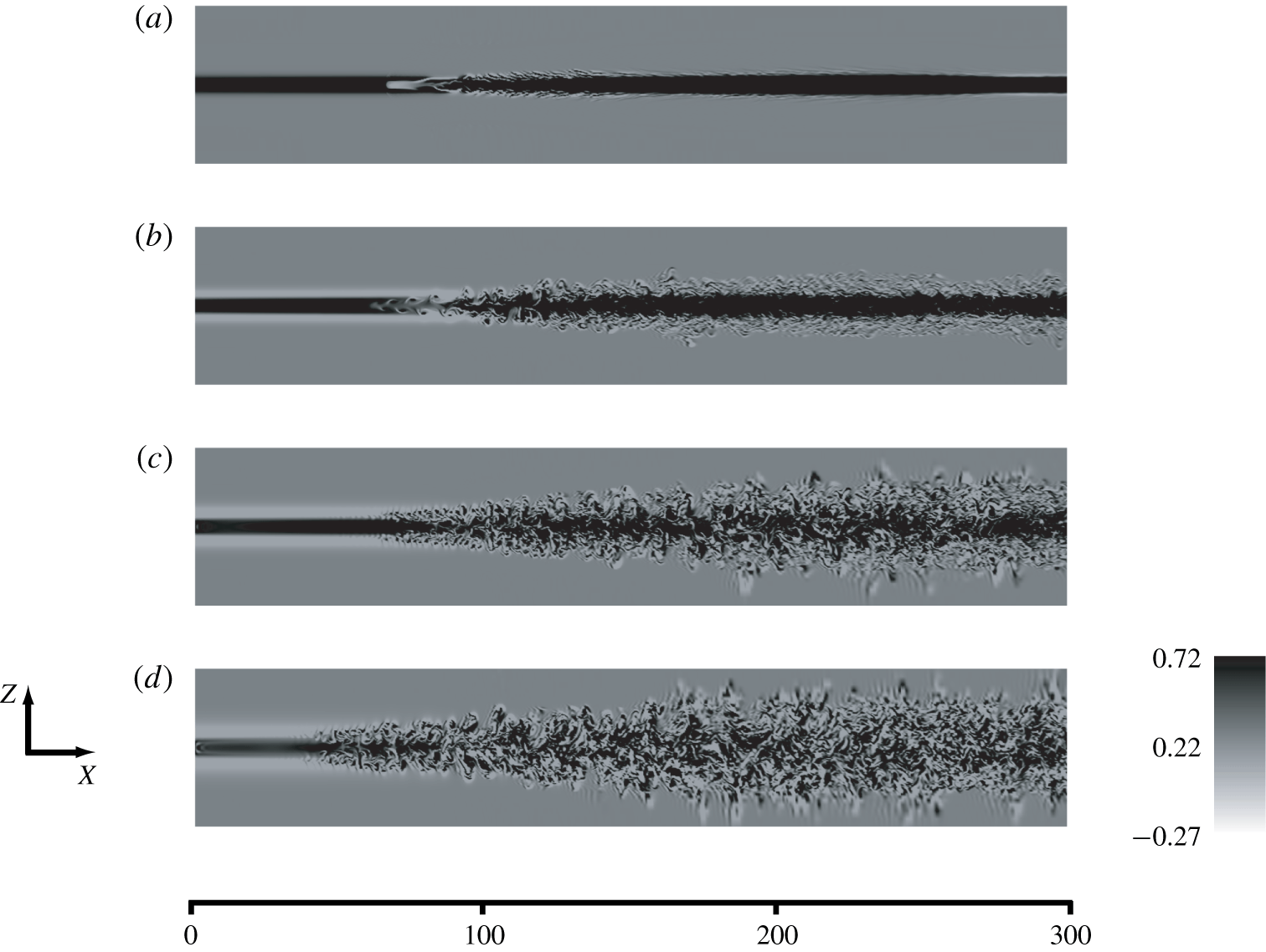
Evolutions of Batchelor vortices ($M_{\infty }=2.5$, $q=0.64,\unicode[STIX]{x1D707}=0.8$) under random disturbance, showing the cross-sections of the helicity density contours along the vortex axis: (a) $D=1.0$, (b) $D=0.5$, (c) $D=0.25$ and (d) $D=0.125$. Positive and negative helicities are rendered in black and white, respectively.

Figure 10.

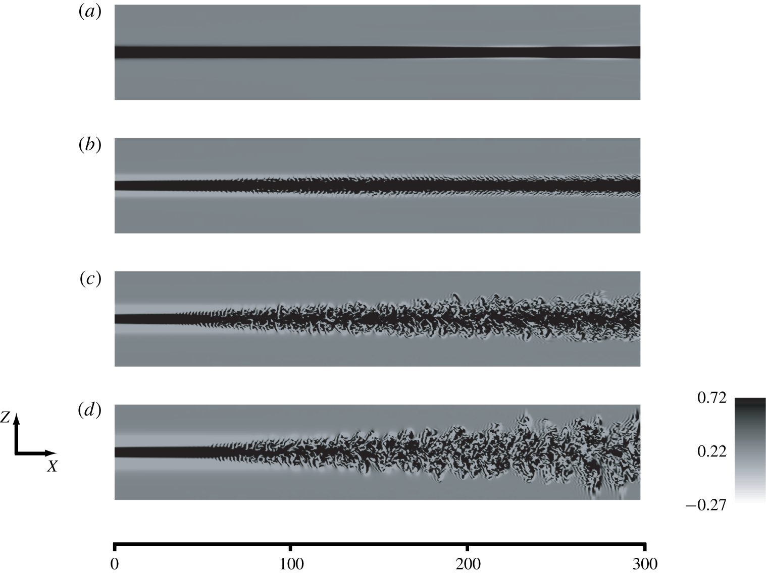
Evolutions of Batchelor vortices ($M_{\infty }=5.0$, $q=0.36,\unicode[STIX]{x1D707}=0.8$) under random disturbance, showing the cross-sections of the helicity density contours along the vortex axis: (a) $D=1.0$, (b) $D=0.5$, (c) $D=0.25$ and (d) $D=0.125$. Positive and negative helicities are rendered in black and white, respectively.

5.1 Effect of helicity instability

This subsection describes the nonlinear evolutions of Batchelor vortices associated with helicity instability. Helicity contours provide useful information about the transition processes of vortices. The spatial developments of a Batchelor vortex with large $q$ are revealed in figures 9 and 10, which show the helicity density contours in the $x$–$z$ cross-sections along the vortex axis at $M_{\infty }=2.5$ ($q=0.64$, $\unicode[STIX]{x1D707}=0.8$) and $M_{\infty }=5.0$ ($q=0.36$, $\unicode[STIX]{x1D707}=0.8$), respectively. Evidently, helicity has a great effect on vortex structure (Moffatt & Tsinober Reference Moffatt and Tsinober1992).

In the $M_{\infty }=2.5$ case with $D=1.0$, weak instability developed inside the vortex core and along the outer edge of the vortex, but the system was stabilised downstream. Note that a conventional Batchelor vortex with $D=1.0$ is exposed to disturbances that grow near the vortex centre (Delbende & Rossi Reference Delbende and Rossi2005). When $D$ reduced to 0.50, spiral fluctuations developed inside the vortex core, followed by a fluctuation growth near the negative helicity region (see figure 3). Observing the pronounced internal growth in conventional Batchelor vortices and the external growth induced by helicity effects in the evolution is a valuable outcome of this approach. At $D=0.25$, fluctuations developed at the interface between the positive and negative helicity profiles. In the initial development stage, these fluctuations consisted of high wavenumber modes (higher than those obtained from $q=0.16$ (Hiejima Reference Hiejima2015a)). In addition, many small-scale developments (such as incompressible evolutions) occurred downstream. At $D=0.125$, the structure was dominated by small scales on the outer edge of the vortex, and the considerable radial spreading of the fluctuation suggested a growth beyond evolutions due to entropy instability (Hiejima Reference Hiejima2019). This demonstrates a tremendous development as a natural transition in supersonic flows. Thus, the observed vortex evolutions for different values of the parameter $D$ were consistent with the helicity instability features determined in the stability analysis (§ 3.2).

Let us discuss the case of $M_{\infty }=5.0$. In contrast to the case of $M_{\infty }=2.5$, no disturbance growth was seeded from the vortex core, and each vortex was disrupted by helicity instability. At $D=1.0$, the vortex flow was stable with some fluctuations (white regions) at the outer vortex. However, this feature differed from that of asymptotic analysis at high wavenumbers in figure 2(d). At $D=0.50$, clear disturbance growths were induced by the helicity profile. In the early development stage, spiral structures appeared as a wrinkled rim in the cross-sections (see also figure 12). Although the evolution was dominated by helicity instability, the radial spreading fluctuation was weak. At $D=0.25$, the small fluctuations generated from the outer edge of the vortex did not extend to the neighbourhood of the vortex axis, and the spreading rate was weaker than at $D=0.25$ in the $M_{\infty }=2.5$ case. This case showed the earliest transition, consistent with the result in figure 3. When $D$ was further reduced to 0.125, small downstream scales appeared despite the high $M_{\infty }=5.0$. Jacquin & Pantano (Reference Jacquin and Pantano2002) showed that turbulence produced within the Batchelor vortex core must overcome the dispersion buffer adjacent to the vortex core before the turbulent fluctuations can reach the vortex periphery. The $D$-dependent helicity instability originally grew at the outer edge of the vortex, suggesting that helicity instability might overcome the rotational stabilization in conventional Batchelor vortices with large $q$.

Figure 11.

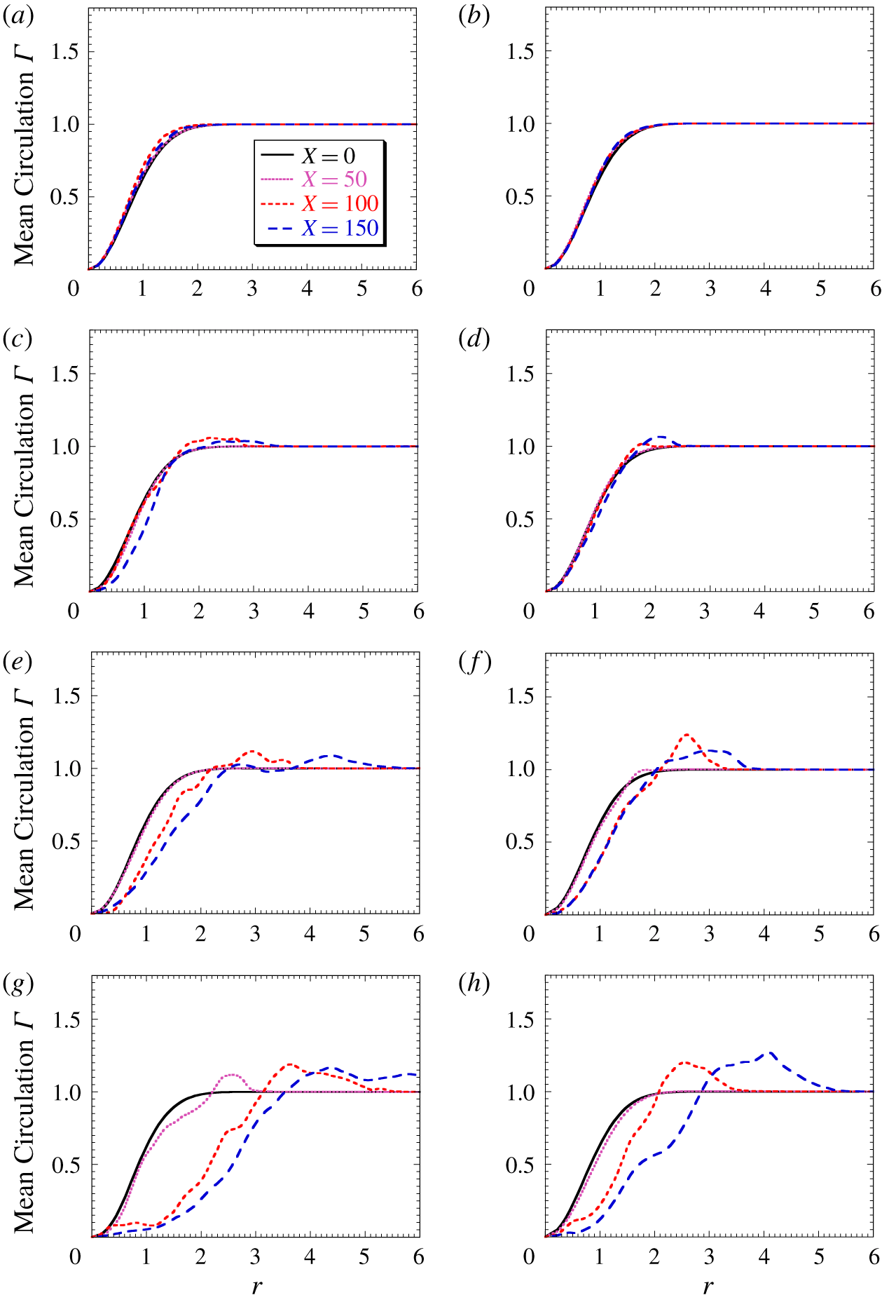
Mean circulation profiles $\overline{\unicode[STIX]{x1D6E4}}/M_{\infty }$: (a,c,e,g) $M_{\infty }=2.5$, $q=0.64$, $\unicode[STIX]{x1D707}=0.8$ and (b,d,f,h) $M_{\infty }=5.0$, $q=0.36$, $\unicode[STIX]{x1D707}=0.8$, and (a,b) $D=1.0$, (c,d) $D=0.50$, (e,f) $D=0.25$, (g,h) $D=0.125$.

5.2 Evolution of circulation profiles and vortical structures

This subsection investigates the difference between helicity instability and the centrifugal instability associated with conventional Batchelor vortices. A centrifugal instability derived by Rayleigh (Reference Rayleigh1917) develops on the circulation profiles of rotational flows (Drazin & Reid Reference Drazin and Reid1981). This instability arises when the mean circulation reduces in the radial direction (Uberoi Reference Uberoi1979) owing to circulation overshoot (Govindaraju & Saffman Reference Govindaraju and Saffman1971) in a turbulent line vortex. Figure 11 shows the mean circulation profiles $\overline{\unicode[STIX]{x1D6E4}}/M_{\infty }$ for various $D$ at $M_{\infty }=2.5$ and 5.0. The circulation profiles were more affected by $D$ than by the Mach number effect. At $D=1.0$, the vortices were stable throughout the spatial evolution. When $D$ reduced to 0.50, weak circulation overshoots indicating centrifugal instability appeared near the vortex core. At $D=0.25$ and 0.125, the circulation overshoot appeared at the outer side of the vortex core, where fluctuations resulted from the helicity profiles. Note that these fluctuations ranged over the regions of phase change ($0<r<4$) in figure 8. In conventional Batchelor vortices, the circulation overshoot decreases with increasing $q$ because the outward spread of fluctuations is suppressed, thereby enhancing the rotational stabilisation (Jacquin & Pantano Reference Jacquin and Pantano2002; Delbende & Rossi Reference Delbende and Rossi2005). However, despite the large $q$, moderate circulation overshoots that characterise small $q$ (Hiejima Reference Hiejima2015a) appear at a point distant from the core. These profiles also differ from the circulation profile of the isentropic vortex at $q=0.16$, which strengthens the centrifugal instability (Hiejima Reference Hiejima2014). It follows that the features of helicity instability differ from those of centrifugal instability.

Figure 12.

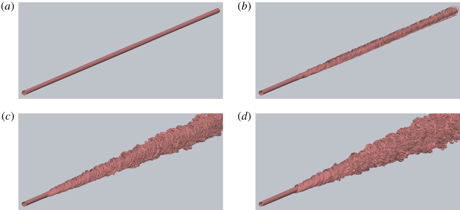
Isosurfaces of the second invariant of the velocity gradient tensor ${\mathcal{Q}}$ at $M_{\infty }=5.0$, $q=0.36$ and $\unicode[STIX]{x1D707}=0.8$: (a) $D=1.0$, (b) $D=0.50$, (c) $D=0.25$ and (d) $D=0.125$.

As described in § 5.1, the spatial evolutions of the vortices at $M_{\infty }=5.0$ and large $D$ apparently differed from those of the linear stability analysis. Figure 12 shows the isosurfaces of the second invariant of the velocity gradient tensor ${\mathcal{Q}}$$(=-0.01)$, which are useful for quantitatively visualising the vortical structures, at $M_{\infty }=5.0$, $q=0.36$, $\unicode[STIX]{x1D707}=0.8$, and four values of $D$. The ${\mathcal{Q}}$ is calculated by

(5.1)$$\begin{eqnarray}{\mathcal{Q}}={\textstyle \frac{1}{2}}(-\unicode[STIX]{x1D61A}_{ij}\unicode[STIX]{x1D61A}_{ij}+\unicode[STIX]{x1D619}_{ij}\unicode[STIX]{x1D619}_{ij}+{\mathcal{P}}^{2}),\end{eqnarray}$$

$$\begin{eqnarray}\unicode[STIX]{x1D61A}_{ij}=\frac{1}{2}\left(\frac{\unicode[STIX]{x2202}u_{j}}{\unicode[STIX]{x2202}x_{i}}+\frac{\unicode[STIX]{x2202}u_{i}}{\unicode[STIX]{x2202}x_{j}}\right),\quad \unicode[STIX]{x1D619}_{ij}=\frac{1}{2}\left(\frac{\unicode[STIX]{x2202}u_{j}}{\unicode[STIX]{x2202}x_{i}}-\frac{\unicode[STIX]{x2202}u_{i}}{\unicode[STIX]{x2202}x_{j}}\right),\quad {\mathcal{P}}=\frac{\unicode[STIX]{x2202}u_{k}}{\unicode[STIX]{x2202}x_{k}},\end{eqnarray}$$

where$\unicode[STIX]{x1D61A}_{ij}$ and $\unicode[STIX]{x1D619}_{ij}$ are the strain rates and vorticity tensors, respectively, which respectively contain the symmetric and asymmetric components of the velocity gradient tensor $\unicode[STIX]{x2202}u_{i}/\unicode[STIX]{x2202}x_{j}$ and ${\mathcal{P}}$ is the divergence of the velocity vectors (Jeong & Hussain Reference Jeong and Hussain1995). As seen in figure 12, the parameter $D$ clearly affected the evolution. At $D=1.0$, the vortex was completely stable, but at $D=0.50$, weak spiral structures appeared after the transition with little outward extension in the radial direction. When $D$ was reduced to 0.25 and 0.125, the vortical structures largely differed from those at $D=0.50$ because strong fluctuation growths were induced by the helicity instability. In the early stage of the evolutions, random disturbances generated spiral structures with a high wavenumber due to the large $q$. At $D=0.125$, the outward spreading was considerably enlarged and the downstream scales were much smaller than in the case of $D=0.25$ (see also figure 10c,d). The eddy generation (in terms of number of eddies) was vastly superior to that of isentropic-vortex effects under uniform stagnation-temperature conditions at $M_{\infty }=5.0$ (Hiejima Reference Hiejima2019). Therefore, these evolution results at small $D$ demonstrate the great effect of helicity instability (term $\text{III}$ in (3.6)).

5.3 Unstable modes selected by random disturbance

From a transition perspective, it is important to understand how modes evolve from random disturbances. This subsection focuses on the growth modes during the vortex development and, hence, elucidates the specific property of Batchelor vortices associated with helicity instability. As shown in figure 6, the axial wavenumber $\unicode[STIX]{x1D6FC}_{r}$ increases with azimuthal wavenumber $m$, implying that the discrimination of the modes in swirling flows is $m$ rather than $\unicode[STIX]{x1D6FC}_{r}$. Thus, the mode decomposition of $m$ was investigated in the spatially developing flows. The flow fluctuations were decomposed by taking the Fourier transform of $m$,

(5.2)$$\begin{eqnarray}\mathscr{F}_{m}(\unicode[STIX]{x1D6F7},x,r,t)=\frac{1}{2\unicode[STIX]{x03C0}}\int _{0}^{2\unicode[STIX]{x03C0}}\unicode[STIX]{x1D6F7}(x,r,t,\unicode[STIX]{x1D703})\text{e}^{\boldsymbol{i}m\unicode[STIX]{x1D703}}\,\text{d}\unicode[STIX]{x1D703},\end{eqnarray}$$

where $\unicode[STIX]{x1D6F7}(x,r,\unicode[STIX]{x1D703})$ represents a physical variable. For the axial vorticity $\unicode[STIX]{x1D6F7}(x,r,\unicode[STIX]{x1D703})=\unicode[STIX]{x1D714}_{x}$, the amplitude of the axial vorticity fluctuation $\unicode[STIX]{x1D6FA}_{x}$ is determined as

(5.3)$$\begin{eqnarray}|\unicode[STIX]{x1D6FA}_{x}|=|\mathscr{F}_{m}(\unicode[STIX]{x1D714}_{x},x,r,t)|.\end{eqnarray}$$

Figure 13.

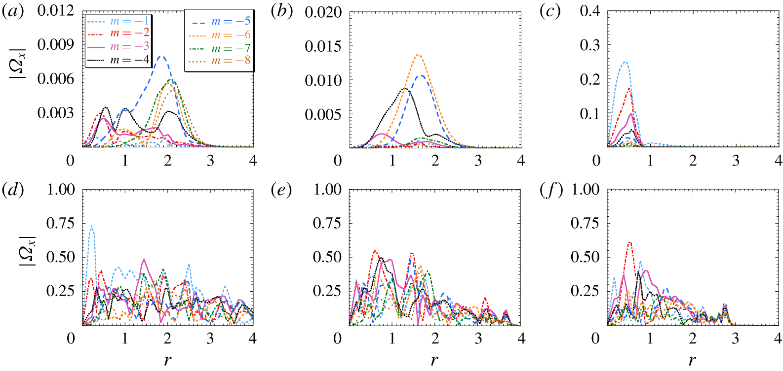
Amplitude profiles of the axial vorticity fluctuations obtained in the mode analysis for various azimuthal wavenumbers at $M_{\infty }=2.5$, $q=0.64$ and $\unicode[STIX]{x1D707}=0.8$: (a) $D=0.125$, $x=30$; (b) $D=0.25$, $x=50$; (c) $D=0.50$, $x=65$; (d) $D=0.125$, $x=100$; (e) $D=0.25$, $x=100$; and (f) $D=0.50$, $x=100$.

Figure 14.

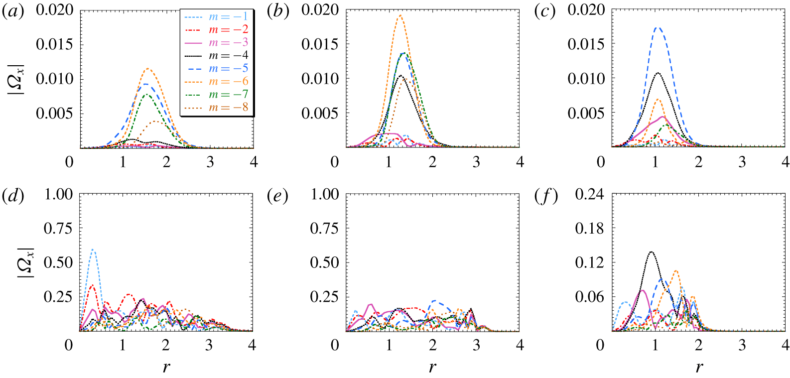
Amplitude profiles of the axial vorticity fluctuations obtained in the mode analysis for various azimuthal wavenumbers at $M_{\infty }=5.0$, $q=0.36$ and $\unicode[STIX]{x1D707}=0.8$: (a) $D=0.125$, $x=50$; (b) $D=0.25$, $x=35$; (c) $D=0.50$, $x=50$; (d) $D=0.125$, $x=100$; (e) $D=0.25$, $x=100$; and (f) $D=0.50$, $x=100$.

Figures 13 and 14 show the amplitude profiles of the axial vorticity fluctuations calculated by (5.3) for eight azimuthal wavenumbers at $M_{\infty }=2.5$ ($q=0.64$, $\unicode[STIX]{x1D707}=0.8$) and $M_{\infty }=5.0$ ($q=0.36$, $\unicode[STIX]{x1D707}=0.8$). In the $M_{\infty }=2.5$ case with $D=0.125$ at $x=30$, some high azimuthal wavenumbers competed around $r=2$. When $D=0.25$ at $x=50$, the peak value of the most unstable mode ($m=-6$) coincided with the extremum of the negative helicity profile in figure 3. These two cases robustly express the feature of helicity instability. In contrast, when $D=0.50$ at $x=65$, the fluctuation growth appeared inside the vortex core ($r<1$; see figure 9b). In addition, the linear unstable mode (exponential growth) was suppressed because low azimuthal wavenumbers dominated in this case; growth of the $m=-1$ mode, which is strongly related to vortex breakdown (Qadri, Mistry & Juniper Reference Qadri, Mistry and Juniper2013), was observed. Abid (Reference Abid2008) suggested that transient growth can trigger nonlinearities near the vortex axis. Thus, this development is not caused by the helicity instability found in § 3. In the cases of $D=0.125$ and 0.25 at $x=100$, fluctuations spread to approximately four times the vortex core. In Batchelor vortices, a large fluctuation on the outer edge of the vortex is necessary to restrain a stabilising mechanism with large $q$ (Jacquin & Pantano Reference Jacquin and Pantano2002). Helicity instability satisfies this necessary condition. Note that the fluctuation amplitude at $x=100$ in these figures is attributed to the changing mean flow in the downstream (see figure 11). Regardless of $D$, the amplitude profiles at $M_{\infty }=5.0$ display the helicity instability feature, namely, several high-azimuthal-wavenumbers grow at the highly sensitive point (negative helicity region) at which the helicity profiles develop instabilities, as shown in the top panels of figure 14. Moreover, the outward spreading was weak at $D=0.50$ (figure 14f). These results accorded with the helicity contours in figure 10. However, for all values of $D$, the magnitudes of these fluctuations were smaller than for $M_{\infty }=2.5$ at $x=100$. Even though helicity instability is observed, the results suggest that there are compressibility effects due to the Mach number in spatial evolutions.

As discussed above, the mode decompositions (except those of figure 13c,f) were characterised by high azimuthal wavenumbers caused by the large $q$ and the helicity profiles. Although vortex breakdown is characterised by a low-wavenumber mode, no supersonic vortex breakdown (i.e. disappearances of the vortex axes (Hiejima Reference Hiejima2017)) appeared in figures 9 and 10. Note that the two cases considered here do not satisfy the onset condition (Hiejima Reference Hiejima2018) because of $q/\unicode[STIX]{x1D707}=0.8$ at $M_{\infty }=2.5$ and $q/\unicode[STIX]{x1D707}=0.45$ at $M_{\infty }=5.0$. Therefore, the present results also support the previous results of vortex breakdown in supersonic flows.

Figures 13 and 14 reveal a predominance of high azimuthal wavenumbers near the minimum of the helicity profiles during the early evolution stage under random noise. Mode selection mechanisms are connected to the local stability properties of flows (Viola et al. Reference Viola, Arratia and Gallaire2016). Understanding how the growth property is governed by natural selection is essential for elucidating the instability phenomena. The maximum growth rate is related to the fluctuations in kinetic energy $\hat{K}$, obtained by integrating the square of the velocity fluctuation $\hat{u} _{k}$,

(5.4)$$\begin{eqnarray}\hat{K}=\int _{A}\frac{1}{2}\overline{\unicode[STIX]{x1D70C}}\,\hat{u} _{k}\hat{u} _{k}\,\text{d}A,\end{eqnarray}$$

where the ‘—’ and ‘$\wedge$’ symbols denote the mean and fluctuating components, respectively, and $A$ is the cross-sectional area in a plane perpendicular to the axial flow at some $x$. The velocity fluctuation $\hat{u} _{k}$ is approximated by

(5.5)$$\begin{eqnarray}\hat{u} _{k}\sim C\text{e}^{-\unicode[STIX]{x1D6FC}_{i}x}.\end{eqnarray}$$

Note that $C$ depends on $y$ and $z$ in the cross-sectional area. Substituting (5.5) into (5.4), $\hat{K}$ is given by

(5.6)$$\begin{eqnarray}\hat{K}\sim \text{e}^{-2\unicode[STIX]{x1D6FC}_{i}x}F(A),\end{eqnarray}$$

where $F(A)$ is found by integrating (5.4) at the given $x$. Taking the logarithm of both sides of (5.6) gives

(5.7)$$\begin{eqnarray}{\textstyle \frac{1}{2}}\log _{e}\hat{K}\sim -\unicode[STIX]{x1D6FC}_{i}\,x+{\textstyle \frac{1}{2}}\log _{e}[F(A)].\end{eqnarray}$$

Differentiating (5.7) and neglecting the last term, we finally obtain

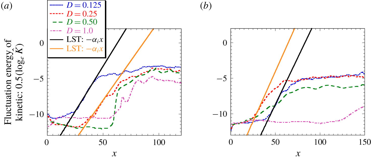
(5.8)$$\begin{eqnarray}{\displaystyle \frac{1}{2}}{\displaystyle \frac{\text{d}}{\text{d}x}}(\log _{e}\hat{K})\sim -\unicode[STIX]{x1D6FC}_{i}.\end{eqnarray}$$

Figure 15.

Streamwise variations in kinetic energy fluctuations ($0.5\log _{e}\hat{K}$) obtained from direct numerical simulations at various $D$ and (a) $M_{\infty }=2.5$, $q=0.64$, $\unicode[STIX]{x1D707}=0.8$ and (b) $M_{\infty }=5.0$, $q=0.36$, $\unicode[STIX]{x1D707}=0.8$. The black ($D=0.125$) and yellow ($D=0.25$) straight lines represent the spatial growth rates $-\unicode[STIX]{x1D6FC}_{i}$ listed in table 1.

Table 1.

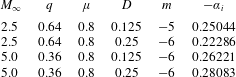
Maximum spatial growth rates $-\unicode[STIX]{x1D6FC}_{i}$ obtained from linear stability analysis in § 3.3.

Figure 15 plots the simulated streamwise variations in the kinetic energy fluctuations ($0.5\log _{e}\hat{K}$) at various $D$ in the $M_{\infty }=2.5$ and $M_{\infty }=5.0$ cases. For comparison, the spatial growth rates $-\unicode[STIX]{x1D6FC}_{i}$ listed in table 1, which are obtained from linear stability analysis in § 3.3, are also plotted as straight lines. Note that the fluctuation magnitude is plotted on the logarithmic scale. In the $M_{\infty }=2.5$ case, the initial energy evolution at $D=0.125$ and 0.25 was dominated by linear unstable modes. However, at $D=0.50$ and 1.0, the energy fluctuations demonstrated the features of nonlinear growth through different transitions. Abid (Reference Abid2008) attributed the discrepancy between the nonlinear evolution and the linear unstable modes to transient growth. As nonlinear effects were negligible at low initial energy, transient growth can be expected in the large energy case ($q=0.64$). In the $M_{\infty }=5.0$ case with $D=0.125$ and 0.25, the linear growth regions were short-lived and the spatial growth rates in the linear stability analysis coincided with the simulation results. At $D=0.50$, the linear growth rate was comparable to that at $D=0.125$ and 0.25 (figure 2b), but the most unstable mode in the linear stability analysis was not contributed to by random noise in the flow (see figure 14c,f). In this case, the helicity instability occurred at the outer side of the vortex core, but was subdued. At $D=1.0$, the growth was slow and weak. Consequently, under the $D\leqslant 0.25$ conditions with a relatively large growth rate, the evolution raised the linear disturbances.