1 Introduction
Consider the following free boundary problem:
 $$ \begin{align} \left\{ \begin{array}{@{}ll} u_t = u_{xx} + u(1-u-k_1v), & 0< x<h(t),\ t>0,\\ v_t = v_{xx} + v(1-v-k_2u), & 0<x<+\infty,\ t>0,\\ v(t,0)=0,\ u(t,0)= u(t,h(t))=0 , & t>0,\\ h'(t) = -u_x (t, h(t)) - \alpha, & t>0,\\ h(0)= h_0,\ \ u(0,x) =u_0 (x),& 0\leq x \leq h_0,\\ v(0,x)=v_0(x),& 0\leq x \leq \infty, \end{array} \right. \end{align} $$
where
 $x=h(t)$
is a moving boundary, and
 $(u(t,x),v(t,x),h(t))$
is to be determined.
 $h_0,\alpha $
and
 $k_i (i=1,2)$
are given positive constants. The initial data
 $v_0$
satisfies

and
 $u_0$
belongs to
 $\mathscr {X}(h_0)$
for some
 $h_0>0$
, where
 $$ \begin{align} \mathscr{X}(h_0)=\left\{ \phi\in C^2([0,h_0]), \phi(0)=\phi(h_0)=0, \ \phi>0 \ in\ [0,h_0)\right \}. \end{align} $$
Ecologically, u is the density of an invasive species and v is the density of a native species density,
 $k_i$
is interspecific competition rate. Free boundary
 ${x=h(t)}$
is the invading front of the invasive species, and it evolves according to the Stefan condition
 $h'(t)=-u_x(t,h(t))-\alpha $
. We use
 $\alpha>0$
to denote the decay rate caused by the bad environment at (or, out of) the boundary such as the food, predators.
When decay rate
 $\alpha =0$
and left boundary condition is Neumann boundary condition, Du and Lin [Reference Du and Lin6] studied the following free boundary problem
 $$ \begin{align} \left\{ \begin{array}{@{}ll} u_t = d_1\Delta u + u(a_1-b_1u-c_1v), & 0< r<h(t),\ t>0,\\ v_t = d_2\Delta v + v(a_2-b_2u-c_2v), & 0<r<+\infty,\ t>0,\\ v_r(t,0)=0,\ u_r(t,0)= u(t,h(t))=0 , & t>0,\\ h'(t) = -u_r (t, h(t)), & t>0,\\ h(0)= h_0,\ \ u(0,r) =u_0 (r),& 0\leq r \leq h_0,\\ v(0,r)=v_0(r),& 0\leq r \leq \infty. \end{array} \right. \end{align} $$
They used this problem to describe the dynamical process of a new competitor u who invades into the habitat of a native species v. The species u spreads through random diffusion in
 $[0,h(t)]$
with spreading front
 $h(t)$
satisfying classical Stefan condition
 $h'(t) = -u_r (t, h(t))$
. They studied the long time behavior of species u and v, and obtained spreading-vanishing dichotomy. In problem (1.1),
 $a_1=b_1=a_2=c_2=1$
,
 $c_1=k_1$
and
 $b_2=k_2$
. For the value of
 $k_i$
, There are the following four cases (for more details, cf. [Reference de Mottoni4, Reference Pao13]):
-
(1)
 $k_i\in (0,1),i=1,2$
;
-
(2)
$0<k_2<1<k_1$
; -
(3)
$0<k_1<1<k_2$
; -
(4)
$k_i\in (1,\infty ),i=1,2$
.


The case (1) is called the weak competition, in this case the competitors co-exist in the future. The case (2) and (3) is usually called weak–strong competition case, while (4) are known as the strong competition cases, but the asymptotic behavior of solutions is difficult to be given clearly. In [Reference Du and Lin6], they considered the case (3) and (4).
There are some other competition systems with free boundaries, such as [Reference Du and Wu8, Reference Wang16, Reference Wang and Zhao18, Reference Wu19]. In [Reference Wu19], they researched the dynamics for a Lotka–Volterra type weak competition system with two free boundaries. Later, [Reference Du and Wu8] investigated the spreading speeds and long time behavior of two invasive species
 $(u,v)$
, where
 $(u,v)$
satisfies
 $$ \begin{align} \left\{ \begin{array}{@{}ll} u_t = u_{xx} + u(1-u-k_1v), & 0< x<h(t),\ t>0,\\ v_t = v_{xx} + v(1-v-k_2u), & 0<x<g(t),\ t>0,\\ v_x(t,0)=0,\ u_x(t,0)= u(t,h(t))=0 , & t>0,\\ h'(t) = -\mu u_x (t, h(t)), \ g'(t)=-\mu v_x(t,g(t)) & t>0,\\ \end{array} \right. \end{align} $$
In [Reference Wang16], they investigated free boundary problems of the prey-predator model with two species living in
 $[0,h(t)]$
, and they satisfy the condition
 $h'(t)=-\mu (u_x(t,x)+\rho v_x(t,x))$
at the same boundary
 $x=h(t)$
. They considered the long time behavior of solution and criteria for spreading and vanishing.
In [Reference Wang and Zhao18], they studied a predator-prey model with double free boundaries, two species satisfy
 $$ \begin{align*}u_t = u_{xx} + u(1-u+av), g(t)< x<h(t) \quad \mbox{and} \quad v_t = dv_{xx} + v(b-v-cu), x \in \mathbb{R}, \end{align*} $$
with free boundary conditions
 $$ \begin{align*}h'(t) = -\mu u_x (t, h(t)), \ g'(t)=-\mu u_x(t,g(t)). \end{align*} $$
They proved a spreading-vanishing dichotomy. Recently, in [Reference Zhang and Wang23], the authors investigated a nonlocal diffusion competition model with seasonal succession and free boundaries. Yang [Reference Yang20] studied a competitive model by considering traveling wave solutions. Besides these, there are also other works concerning free boundary problem of diffusion systems (such as [Reference Haomin, Liu and Wang10, Reference Li and Wang11, Reference Qi, Su and Wang14, Reference Wang and Yao17, Reference Zaw and Wang21]).
If
 $v\equiv 0$
, this means that there are no native species, the systems reduce to the following diffusive problem
 $$ \begin{align} \left\{ \begin{array}{@{}ll} u_t = u_{xx} + u(1-u), & 0< x<h(t),\ t>0,\\ u(t,0)= u(t,h(t))=0 , & t>0,\\ h'(t) = -u_x (t, h(t)) - \alpha, & t>0,\\ h(0)= h_0,\ \ u(0,x) =u_0 (x),& 0\leq x \leq h_0. \end{array} \right. \end{align} $$
Such a similar problem is studied in [Reference Cai, Lou and Zhou3] with decay rate
 $\alpha>0$
. It is more difficult for the solution to spread than the case
 $\alpha =0$
. Since
 $h'(t)>0$
only if
 $u_x(t,h(t))<-\alpha $
. They obtained a different vanishing and a transition case. Also, [Reference Cai1, Reference Cai and Gu2, Reference Ding, Cai and Xu5] studied such problems with
 $\alpha>0$
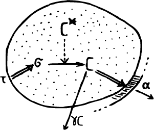
representing the decay rate caused by the bad environment at the boundary, such as food, predators and so on. Moreover, such a boundary condition are often used in the growth of protocell (cf. [Reference Friedman and Hu9, Reference Zhang, Qu and Hu22]), in the process of diffusion and polymerization of building materials, there is a disintegration (denoted by
 $\alpha $
) produced by many factors, such as aging. So the boundary condition satisfies
 $$ \begin{align*}V_n = -\frac{\partial u}{\partial n} - \alpha, \end{align*} $$
where
 $V_n$
is the velocity in the direction n, see Figure 1. In one-dimensional space, this condition is our condition used in the problem (1.1). Such a boundary condition is also used the tumour model.
The growth of the protocell model.

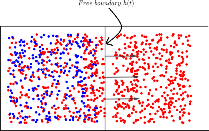
In this article, we will consider the spreading of two species u and v. There is new species u invading into an environment where a native competitor v already exists on the whole space, see Figure 2. The survival interval of the species v is
 $[0,+\infty ]$
, while the survival interval of u is
 $[0,h(t)]$
. Since u is moving depending the food, the density of u and other factors, so the survival boundary of u, i.e.,
 $h(t)$
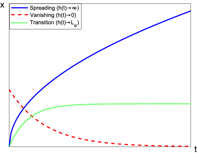
is often depending on time t, there are three situations for the limits of
 $h(t)$
, i.e., 0,
 $+\infty $
or a finite number, see Figure 3.
The spreading of two species u and v.

The limits of free boundary
 $h(t)$
.

The situations of spreading of these two species u and v are complicated, we only consider two cases for interspecific competition rate:
 $0{\kern-0.5pt}<{\kern-0.5pt}k_2{\kern-0.5pt}<{\kern-0.5pt}1{\kern-0.5pt}<{\kern-0.5pt}k_1$
and
 $0{\kern-0.5pt}<{\kern-0.5pt}k_1{\kern-0.5pt}<{\kern-0.5pt}1{\kern-0.5pt}<{\kern-0.5pt}k_2$
; Usually, there is a decay rate at the boundary, we will analysis such decay rate
 $\alpha $
how to affect the spreading of two species. Besides, we will show that the initial data of u plays an crucial role in the asymptotic behavior of two species.
From [Reference Cai and Gu2, Reference Wang16, Reference Wang and Zhao18], the problem (1.1) has a unique solution
 $(u,v,h)$
, with
 $ v(t,x) \in C^{(1+\varrho )/2,1+\varrho }([0,+\infty )\times [0,+\infty ))$
,
 $u(t,x) \in C^{(1+\varrho )/2,1+\varrho }([0,T]\times [0,h(t)])$
,
 $h(t) \in C^{1+\varrho /2}([0,T])$
, where
 $\varrho \in (0,1)$
,
 $T\in (0,+\infty ]$
. In the following, we show that in some cases
 $T<+\infty $
and for other cases
 $T=+\infty $
, this depends on the initial data. However, as in the proof of [Reference Cai, Lou and Zhou3], the limit
 $h_T:=\lim _{t\to T}h(t)\in [0,+\infty ]$
exists. In particular, we also write
 $h_T$
as
 $h_\infty $
when
 $T=+\infty $
.
In this article, we have the following two main results.
Main result 1 (Theorem 3.2)
When
 $0<k_2<1<k_1$
, we have the following results for the spreading of
 $(u,v)$
:
 $$ \begin{align} T<+\infty, \ \lim_{t \to T} h(t)=0, \ \lim_{t \to T}\max _{x\in [0,h(t)]}u(t,x)=0 \end{align} $$
and
 $$ \begin{align} \lim_{t \to +\infty}v(t,x)=\Lambda(x) \quad \mbox{locally uniformly for } x\in [0,+\infty), \end{align} $$
where
 $\Lambda (x)$
satisfies
 $$ \begin{align} \left\{ \begin{array}{@{}ll} \Lambda"+\Lambda(1-\Lambda)=0,& x>0,\\ \Lambda(0)=0, \ \Lambda(+\infty)=1. \end{array} \right. \end{align} $$
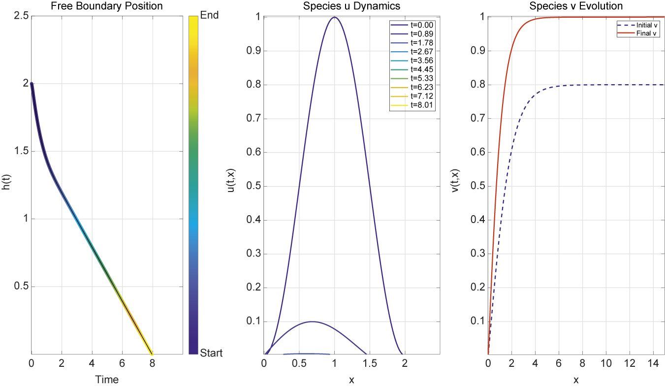
Remark 1.1 To explain the results of main results 1(i.e., Theorem 3.2), we give the numerical results by taking
 $k_1=2, \ k_2=0.3 \ \alpha =0.2$
and
 $h_0=2$
, see Figure 4.
Numerical simulations of
 $(u,v,h)$
are shown, from left to right, they are: the shrinking of free boundary
 $h(t)$
when u vanishes, vanishing of u, the spreading of v.

Main result 2 (Theorem 4.1)
When
 $0<k_1<1<k_2$
and
 $0<\alpha <\alpha _0:=\sqrt {3}/3$
, we have, the solution
 $(u,v,h)$
is either in
-
Case (I): spreading of u and vanishing of v:
$T=+\infty $
,
$\lim _{t \to +\infty }u(t,\cdot )=\Lambda (\cdot )$
and
$\lim _{t \to +\infty }v(t,\cdot )=0$
uniformly in any bounded subset of
$[0,+\infty )$
;or
-
Case (II): vanishing of u and spreading of v: (1.7) and (1.8) hold;
or
-
Case (III): in the transition case:
$h_\infty =L_\alpha $
,
$u (t,\cdot )\to w_\alpha (\cdot )$
locally uniformly in
$(0,h_\infty )$
and
$ v(t,\cdot ) \to \eta _\alpha (\cdot )$
locally uniformly in
$(0, +\infty )$
, where
$(w_\alpha ,\eta _\alpha ,L_\alpha )$
is the solution of (1.10)
$$ \begin{align} \left\{ \begin{array}{@{}ll} -w"=w(1-w-k_1\eta), \quad 0<x<+\infty,\\ -\eta"=\eta(1-\eta-k_2w), \quad 0<x<+\infty,\\ w(0)=w(L_\alpha)=0,\ -w'(L_\alpha)=\alpha,\\ w(x)>0 \ for \ x\in(0,L_\alpha), \\ w(x)\equiv 0 \ for \ x\geq L_\alpha,\\ \eta(0)=0, \eta(+\infty)=1. \end{array} \right. \end{align} $$


Moreover, for the initial data
 $u_0=\sigma \phi $
with
 $\phi \in \mathscr {X}(h_0)$
, we prove that there is a critical data
 $\sigma ^{*}$
such that Case (I) holds when
 $\sigma>\sigma ^{*}$
, Case (II) holds when
 $\sigma < \sigma ^{*}$
, and Case (III) holds when
 $\sigma = \sigma ^{*}$
.
Remark 1.2 The existence of the solution
 $(w_\alpha ,\eta _\alpha ,L_\alpha )$
is given in Lemma 2.7. When
 $\alpha \geq \alpha _0$
, there is no compactly solution.
We organized this article as follows. In Section 2, we give the general existence and uniqueness results, and the comparison principle. In Sections 3 and 4, we study the long time behavior of solutions when
 $0<k_1<k_2$
and
 $0<k_2<k_1$
respectively. In Section 5, we give some sufficient conditions for spreading, vanishing and transition, and complete the proof main results.
2 Preliminary results
In this section, we first prove a local existence and uniqueness result for the problem (1.1). Consider the following general free boundary problem
 $$ \begin{align} \left\{ \begin{array}{@{}ll} u_t = u_{xx} + f(u,v), & 0< x<h(t),\ t>0,\\ v_t = v_{xx} + g(u,v), & 0<x<+\infty,\ t>0,\\ v(t,0)=0,\ u(t,0)= u(t,h(t))=0 , & t>0,\\ h'(t) = -u_x (t, h(t)) - \alpha, & t>0,\\ h(0)= h_0,\ \ u(0,x) =u_0 (x),& 0\leq x \leq h_0,\\ v(0,x)=v_0(x),& 0\leq x \leq \infty, \end{array} \right. \end{align} $$
where
 $f(0,v)=g(u,0)=0$
for any
 $u,v\in \mathbb {R}$
,
 $u_0$
belongs to
 $\mathscr {X}(h_0)$
and
 $v_0$
satisfies (1.2).
Theorem 2.1 Assume that f and g are locally Lipschitz continuous in
 $\mathbb {R}^2_+$
. For any
 $\varrho \in (0,1)$
,
 $u_0 \in \mathscr {X}(h_0)$
and
 $v_0$
satisfies (1.2), there exists
 $T>0$
such that problem (2.1) admits a unique bounded solution defined on
 $[0,T)$
with
 $T\in [0,+\infty ]$
and
 $$ \begin{align} (u,v,h)\in C^{(1+\varrho)/2,1+\varrho}(D_T)\times C^{(1+\varrho)/2,1+\varrho}(D^\infty_T)\times C^{1+\varrho/2}([0,T]), \end{align} $$
moreover,
 $$ \begin{align*}{\Vert u \Vert}_{C^{(1+\varrho)/2,1+\varrho}(D_T)}+{\Vert v \Vert}_{C^{(1+\varrho)/2,1+\varrho}(D_T^\infty)}+{\Vert h\Vert}_{C^{1+\varrho/2,1+\varrho}([0,T])}\leq C,\end{align*} $$
where
 $D_T=\{(t,x)\in \mathbb {R}^2:t\in [0,T], \ x\in [0,h(t)]\}$
,
 $D_T^\infty =\{(t,x)\in \mathbb {R}^2:t\in [0,T], x\in [0,+\infty )\}$
, C and T only depend on
 $h_0,\varrho ,{\Vert u_0 \Vert }_{{C^2}([0,h_0])},{\Vert v_0 \Vert }_{{C^2}([0,\infty ))}$
and the local Lipschitz coefficients of
 $f,g$
.
Theorem 2.2 Under the assumptions of Theorem 2.1, if we assume further that there exists a constant
 $L>0$
such that
 $f(u,v)\leq L(u+v)$
and
 $g(u,v)\leq L(u+v)$
for
 $u,v\geq 0$
, then the unique solution
 $v(t,x)$
obtained in Theorem 2.1 can be extended uniquely to all
 $t>0$
, and if
 $\inf \limits _{0<t<T}h(t)>0$
, then the solution can be extended to a bigger interval
 $(0,T_{*})$
with
 $T_{*}>T$
.
Remark 2.3 We only consider the long time behavior of bounded solutions, so conditions in Theorem 2.2 is used to exclude the possibility that
 $(u,v)$
blows up in finite time. Of course, the problem (1.1) satisfies conditions in Theorem 2.2. Recall that we introduce
 $\alpha>0$
in the free boundary condition. The property
 $h'(t)>0$
in case
 $\alpha =0$
(as shown in [Reference Cai, Lou and Zhou3]) is no longer necessarily to be true. On the contrary, in some cases, the domain
 $[0,h(t)]$
may shrink, even, to a point.
By Theorems 2.1 and 2.2, we have the following estimates.
Theorem 2.4 Problem (1.1) admits a unique and uniformly bounded solution
 $(u,v,h)$
satisfying (2.2). And the solution
 $v(t,x)$
can be extended to all
 $t>0$
and
 $u(t,x)$
is defined on
 $[0,T)$
with
 $T\in (0,+\infty ]$
. Moreover, there exist constants
 $M_1$
and
 $M_2$
such that
 $$ \begin{align*}0<u(t,x)&\leq M_1 \ \ \mathit{for}\ t\in [0, T), \ 0\leq x<h(t),\\0<v(t,x)&\leq M_2 \ \ \mathit{for}\ t\in [0,+\infty), \ 0\leq x<+\infty.\end{align*} $$
And, there exists a constant
 $M_3$
such that
 $$ \begin{align*}-\alpha<h'(t)\leq M_3 \ \ for \ t\in (0,T).\end{align*} $$
Proof From Theorems 2.1 and 2.2, the problem (1.1) admits a unique solution
 $(u,v,h)$
satisfying (2.2), and
 $v(t,x)$
is defined for all
 $t>0$
,
 $u(t,x)$
can be extended to
 $t\in [0,+\infty )$
as long as
 $h(t)>0$
for
 $t>0$
.
It follows from the comparison principle that
 $u(t,x)\leq \bar {u}(t)$
for
 $t\in (0,T)$
and
 $x\in [0,h(t)]$
, where
 $$ \begin{align*}\bar{u}(t):=e^t\left(e^t-1+\frac{1}{{\Vert u_0 \Vert}_\infty}\right)^{-1}\end{align*} $$
which is the solution of the problem
 $$ \begin{align} \left\{ \begin{array}{@{}ll} \displaystyle \frac{d\bar{u}}{dt}=\bar{u}(1-\bar{u}), & t>0,\\ \bar{u}(0)={\Vert u_0 \Vert}_\infty. \end{array} \right. \end{align} $$
Thus we have
 $$ \begin{align*} u(t,x)\leq M_1:= \sup \bar{u}(t), \; t>0. \end{align*} $$
Since
 $v(t,x)$
satisfies
 $$ \begin{align*}\left\{ \begin{array}{@{}ll} v_t-v_{xx}\geq v(1-v),& t>0, \; 0\leq x<+\infty,\\ v(0,x)=v_0(x)\geq 0, & 0\leq x<+\infty. \end{array} \right.\end{align*} $$
We have
 $v(t,x)\leq M_2 := \max\{{\Vert v_0\Vert }_{L^\infty (0,+\infty )},1\}$
.
Using the strong maximum principle to the equation of u we obtain
 $$ \begin{align*}u(t,x)>0 \ for \ \ t\in (0,T), \ 0< x<h(t),\end{align*} $$
and
 $v(t,x)>0$
for
 $t>0,\ 0< x<\infty $
.
Additionally, to estimate the boundness of
 $h(t)$
, we construct the function
 $$ \begin{align} \widetilde{U}(t,x):=M_1[2M(h(t)-x)-M^2(h(t)-x)^2] \end{align} $$
defined on
 $$ \begin{align*}Q:=\{(t,x):0<t<\widetilde{T}, \max\{h(t)-M^{-1},0\}<x<h(t)\},\end{align*} $$
where
 $$ \begin{align*}M:= \max\left \{ \frac{\alpha+\sqrt{\alpha^2+2}}{2}, \frac{4{\Vert u_0 \Vert}_{C^1([-h_0,h_0])}}{3C_1} \right \}.\end{align*} $$
By a direct calculation,
 $0\leq \widetilde {U} \leq M_1$
in Q. The definitions of
 $\widetilde {U}$
and M imply that
 $$ \begin{align*}\widetilde{U}_t-\widetilde{U}_{xx}-\widetilde{U}(1-\widetilde{U})\geq C_1(2M^2-2M\alpha-1)\geq 0 \ \ in \ Q.\end{align*} $$
Additionally, when
 $h(t)\geq M^{-1}$
,
 $$ \begin{align*}\left\{ \begin{array}{@{}ll} \widetilde{U}(t,h(t))=u(t,h(t))=0, \quad t\in(0,\widetilde{T}),\\ u_0(x)\leq \widetilde{U}(0,x),\quad x\in [h_0-M^{-1},h_0]\cap[-h_0,h_0],\\ \widetilde{U}(t,h(t)-M^{-1})=M_1\geq u(t,h(t)-M^{-1}), \end{array} \right.\end{align*} $$
and
 $$ \begin{align*}\widetilde{U}(t,0)>0=u(t,0).\end{align*} $$
Hence, it derives from the comparison principle that
 $u(t,x)\leq \widetilde {U}(t,x)$
in Q. Therefore,
 $$ \begin{align*}h'(t)=-u_x(t,h(t))-\alpha \leq U_x(t,h(t))-\alpha = 2M_1M-\alpha :=M_3\\[-33pt] \end{align*} $$
For given a pair of functions
 $\mathbf {\underline {u}}:=(\underline {u},\underline {v})$
and
 $\mathbf {\overline {u}}:=(\overline {u},\overline {v})$
, denote
 $$ \begin{align*}[\mathbf{\overline{u}},\mathbf{\underline{u}}]=\{ \mathbf{u}:=(u,v)\in[C([0,T]\times [0,+\infty))]^2 : (\underline{u},\underline{v})\leq(u,v)\leq (\overline{u},\overline{v})\}.\end{align*} $$
For
 $(u_1,v_1)\leq (u_2,v_2)$
, we mean
 $u_1\leq u_2$
and
 $v_1\leq v_2$
.
We next give the comparison principle for general case which includes the problem (1.1). That is
 $f(u,v)=u(1-u-k_1v)$
and
 $g(u,v)=v(1-v-k_2u)$
.
Lemma 2.5 (The Comparison Principle)
Let
 $(f,g)$
be quasimonotone nonincreasing and Lipschitz continuous in
 $[\mathbf {\overline {u}},\mathbf {\underline {u}}]$
, with
 $f(0,v)=g(u,0)=0$
. Assume that
 $T\in [0,+\infty )$
,
 $\underline {h}$
,
 $\overline {h}\in C^1([0,T])$
,
 $$ \begin{align*}\underline{u}\in C(\overline{\Sigma_T^1})\cap C^{1,2}(\Sigma_T^1) \ with \ \Sigma_T^1:=\{(t,x)\in \mathbb{R}^2: t\in (0,T], \ x\in (0,\underline{h}(t))\},\end{align*} $$
 $$ \begin{align*}\overline{u}\in C(\overline{\Sigma_T^2})\cap C^{1,2}(\Sigma_T^2) \ with \ \Sigma_T^2:=\{(t,x)\in \mathbb{R}^2: t\in (0,T], \ x\in (0,\overline{h}(t))\},\end{align*} $$
 $$ \begin{align*}\underline{v},\overline{v}\in(L^\infty\cap C)([0,T]\times[0,\infty))\cap C^{1,2}((0,T]\times [0,+\infty)),\end{align*} $$
and
 $\underline {u},\overline {u},\underline {v},\overline {v}\geq 0, \ h(0)>0$
, such that
 $$ \begin{align} \left\{ \begin{array}{@{}ll} \overline{u}_t-\overline{u}_{xx}\geq f(\overline{u},\underline{v}),&0<t\leq T, \ 0\leq x< \overline{h}(t),\\\underline{u}_t-\underline{u}_{xx}\leq f(\underline{u},\overline{v}),&0<t\leq T, \ 0\leq x< \underline{h}(t),\\\overline{v}_t-\overline{v}_{xx}\geq g(\underline{u},\overline{v}),&0<t\leq T, \ 0\leq x< +\infty,\\\underline{v}_t-\underline{v}_{xx}\leq g(\overline{u},\underline{v}),&0<t\leq T, \ 0\leq x< +\infty,\\\overline{u}(t,0)=\underline{v}(t,0)=0, \ \overline{u}(t,x)=0,& 0<t\leq T, \ \overline{h}(t)\leq x<+\infty,\\\underline{u}(t,0)=\overline{v}(t,0)=0, \ \underline{u}(t,x)=0,& 0<t\leq T, \ \underline{h}(t)\leq x<+\infty,\\\underline{h}'(t)\leq -\underline{u}_x(t,h(t))-\alpha,&0<t\leq T,\\\overline{h}'(t)\geq -\overline{u}_x(t,h(t))-\alpha,&0<t\leq T,\\\underline{h}(0)\leq h_0\leq \overline{h}(0),\\\underline{u}_0(x)\leq u_0(x)\leq \overline{u}_0(x),& 0\leq x\leq h_0,\\\underline{v}_0(x)\leq v_0(x)\leq \overline{v}_0(x),& 0\leq x\leq +\infty. \end{array} \right. \end{align} $$
Let
 $(u,v,h)$
be the unique bounded solution of (2.1) with initial data
 $(u_0,v_0)$
. Then
 $\underline {h}(t)\leq h(t))\leq \overline {h}(t)$
in
 $(0,T]$
,
 $\underline {u}(t,x)\leq u(t,x)\leq \overline {u}(t,x)$
for
 $(t,x)\in (0,T]\times [0,h(t))$
and
 $\underline {v}(t,x)\leq v(t,x)\leq \overline {v}(t,x)$
for
 $(t,x)\in (0,T]\times [0,+\infty )$
.
Remark 2.6 If
 $\alpha $
in (2.5)
 $_7$
is replaced by some
 $\beta>\alpha $
, or/and
 $\alpha $
in (2.5)
 $_8$
is replaced by some
 $\gamma < \alpha $
, the conclusions of Lemma 2.5 are also true. We call
 $(\overline {u},\underline {v})$
(resp.
 $(\underline {u},\overline {v})$
) is the upper solution (resp. lower solution).
Lemma 2.7 Assume
 $0<k_1<1<k_2$
and
 $0<\alpha <\alpha _0:=\sqrt {3}/3$
, the problem (1.10) has a solution
 $(w_\alpha ,\eta _\alpha ,L_\alpha )$
.
Proof By the phase plane analysis (cf. [Reference Cai and Gu2]), there exists
 $L^{*}_1$
, for any
 $L>L^{*}_1$
, the problem
 $$ \begin{align} \left\{ \begin{array}{@{}ll} -\bar{w}"=\bar{w}(1-\bar{w}), & 0<x<L,\\ \bar{w}(0)=\bar{w}(L)=0 \end{array} \right. \end{align} $$
has a unique compactly supported solution, denoted by
 $w_c^{(1)}$
, and
 $-w_c^{(1)}(L)>0$
,
 $-w_c^{(1)}(L) < \alpha _0:= -w^{\prime }_\infty (0)$
, where
 $w_\infty $
is the solution of
 $$ \begin{align} \left\{ \begin{array}{@{}ll} -w"=w(1-w), \quad 0<x<+\infty,\\ w(0)=0, \ w(+\infty)=1. \end{array} \right. \end{align} $$
Actually, from [Reference Cai1, Theorem 2.5], we have
 $w^{\prime }_\infty (0) = \sqrt {3}/3$
, for any
 $\alpha \in (0,\alpha _0)$
, there is a
 $l_\alpha $
such that the problem (2.6) has a solution with
 $-\bar {w}'(l_\alpha )=\alpha $
. And there is no compactly solution when
 $\alpha \geq \alpha _0$
.
Also, there exists
 $L^{*}_2$
, for any
 $L>L^{*}_2$
, the problem
 $$ \begin{align} \left\{ \begin{array}{@{}ll} -\underline{w}"=\underline{w}(1-\underline{w}-k_1), & 0<x<L,\\ \underline{w}(0)=\underline{w}(L)=0, \end{array} \right. \end{align} $$
has a unique compactly supported solution, denoted by
 $w_c^{(2)}$
. Denote the solution of
 $$ \begin{align} \left\{ \begin{array}{@{}ll} -\bar{\eta}"=\bar{\eta}(1-\bar{\eta}), & 0<x<+\infty,\\ \bar{\eta}(0), \ \bar{\eta}(+\infty) =1, \end{array} \right. \end{align} $$
as
 $\bar {\eta }(x)$
. By the standard upper and lower solutions method, there is
 $L_0^{*}$
, for
 $l>L_0^{*}$
the problem
 $$ \begin{align} \left\{ \begin{array}{@{}ll} -w"=w(1-w-k_1\eta), \quad x>0,\\ -\eta"=\eta(1-\eta-k_2w), \quad x>0,\\ w(0)=w(l)=\eta(0)=0, \ w(x)>0, \ 0<x<l,\\ w(x) \equiv 0, x \geq l \end{array} \right. \end{align} $$
has at least one positive solution, denoted by
 $(w_l,\eta _l)$
and
 $$ \begin{align*}w_c^{(2)}(x)\leq w_l(x) \leq w_c^{(1)}(x),\quad 0 \leq \eta_l(x)\leq \bar{\eta}(x), \quad 0<x<l.\end{align*} $$
Moreover,
 $w_l^{\prime }(0)>0$
 $-w^{\prime }_l(l)>0$
, and
 $w^{\prime }_l(l) \to 0$
as
 $l \to L_0^{*}$
.
For any small
 $\varepsilon>0$
,
 $(w_l,\eta _l)$
also satisfies
 $$ \begin{align} \left\{ \begin{array}{@{}ll} -w"=w(1-w-k_1\eta), \quad 0<x<l,\\ -\eta"=\eta(1-\eta-k_2w), \quad 0<x<l,\\ w(0)=w(l)=\eta(0)=0, \ w(x)>0, \ 0<x<l,\\ w(x) \equiv 0, x \geq l, \ \eta(l)\leq 1+\varepsilon. \end{array} \right. \end{align} $$
Letting
 $l \to +\infty $
, then
 $(w_l,\eta _l) \to (w_\infty ,0)$
, where
 $w_\infty $
is the solution of (2.7), and
 $w^{\prime }_\infty (0)=\sqrt {3}/3$
.
For any
 $\alpha \in (0,\alpha _0)$
, there is
 $l=L_\alpha $
such that the problem (2.10) has a solution satisfying
 $-w'(L_\alpha ) = \alpha $
. Denote such solution as
 $(w_\alpha ,\eta _\alpha ,L_\alpha )$
, that is, the solution of the problem (1.10).
3 Invasion of an inferior competitor
In this section, we consider the situation that
 $0<k_2<1<k_1$
, namely u is an inferior competitor. In this case, we analyze the asymptotic behavior of
 $(u,v)$
and show that the inferior invader vanishes at last while the superior species always survives the invasion.
Lemma 3.1 Let
 $(u,v,h)$
be a solution of the problem (1.1).
 $(u,h)$
is defined on
 $[0,\widetilde {T})$
with
 $\widetilde {T}\in (0,+\infty ]$
. If
 $\ \lim _{t\to \widetilde {T}}h(t)=0$
, then
 $\widetilde {T} <+\infty $
and
 $$ \begin{align*}\lim_{t\to \widetilde{T}}\mathop{\max}_{0\leq x \leq h(t)}u(t,x)=0.\end{align*} $$
Proof From Theorem 2.4, we have
 $u(t,x) \leq M_1$
for all
 $x\in [0,h(t)]$
and
 $t\in [0,T]$
. Using the upper solution
 $\widetilde {U}(t,x)$
constructed in Theorem 2.4. Note that
 $\lim _{t \to \widetilde {T}}h(t)=0$
, then there exists
 $T_1<\widetilde {T}$
such that
 $h(t)-M^{-1}<0$
for
 $t>T_1$
. Therefore
 $u(t,x)\leq \widetilde {U}(t,x)$
for
 $t>T_1$
and
 $x\in [0,h(t)]$
. Thus we have
 $$ \begin{align*}\widetilde{U}(t,x)\leq C_1[2Mh(t)-M^2h^2(t)]\to 0 \ \ as \ t\to \widetilde{T}.\end{align*} $$
From this and
 $u(t,x)\leq \widetilde {U}(t,x)$
, we have
 $$ \begin{align} {\Vert u(t,\cdot) \Vert}_{L^\infty([0,h(t)])}\to 0 \ \ as \ t\to \widetilde{T}. \end{align} $$
We now prove that
 $\widetilde {T}<+\infty $
and
 $\lim _{t \to +\widetilde {T}}h(t)=0$
. For
 $\varepsilon _{*}\leq \frac {\alpha }{4M}$
, by (3.1), there exists
 $0<T_2<\widetilde {T}$
such that and
 $h(t)-M^{-1}<0$
and
 $u(t,x)\leq \varepsilon _{*}$
. The function
 $$ \begin{align*}\widetilde{U}_2(t,x):=\varepsilon_{*}[2M(h(t)-x)-M^2(h(t)-x)^2],\ x\in [0,h(t)]\end{align*} $$
is also an upper solution for
 $u(t,x)$
. Therefore
 $u(t,h(t))\leq \widetilde {U}_2(t,x)$
for
 $x\in [0,h(t)]$
and
 $t>T_2$
. Hence we have
 $$ \begin{align*}-u_x(t,h(t))\leq- \left(\widetilde{U}_2\right)_x(t,h(t))=2M\varepsilon_{*}\leq\frac{\alpha}{2}.\end{align*} $$
Hence
 $h'(t) = -u_x(t,h(t))-\alpha \leq -\frac {\alpha }{2}$
, this means that
 $ h(t)\to 0$
as
 $t\to \widetilde {T}\leq \frac {2h_0}{\alpha }$
.
Theorem 3.2 Let
 $(u,v,h)$
be the solution of (1.1),
 $(u,h)$
defined on
 $[0,T)$
with
 $T\in [0,+\infty ]$
, if
 $\ 0<k_2<1<k_1$
and
 , then u vanishes:
 $$ \begin{align*}T<+\infty, \ \lim_{t\to T} \mathop{\max}_{x\in[0,h(t)]}u(t,x)=0, \ \lim_{t\to T}h(t)=0,\end{align*} $$
and v spreads:
 $$ \begin{align*}\lim_{t\to +\infty}v(t,x)=\Lambda(x) \ \mathit{locally\ uniformly \ for} \ x\in[0,+\infty), \end{align*} $$
where
 $\Lambda (x)$
satisfies (1.9).
Proof We assume
 $T=+\infty $
. From Theorem 2.4, we have
 $u(t,x)\leq \bar {u}(t)$
for
 $t>0$
and
 $x\in [0,h(t)]$
. Since
 $\lim _{t \to +\infty }\bar {u}(t)=1$
, we deduce that
 $$ \begin{align*}\limsup_{t\to +\infty}u(t,x)\leq 1 \ \mathit{uniformly\ for} \ x\in[0,\infty).\end{align*} $$
Furthermore, consider the parabolic problem
 $$ \begin{align} \left\{ \begin{array}{@{}ll} \varPhi_t-\varPhi_{xx}=\varPhi(1-\varPhi),& t>0, \ x>0,\\ \varPhi(t,0)=0, & t>0,\\ \varPhi(0,x)= u_0(x),& x>0. \end{array} \right. \end{align} $$
Letting
 $t\to +\infty $
we have
 $$ \begin{align} \varPhi(t,\cdot)\to \Lambda(\cdot) \ in \ C^2[0,+\infty], \end{align} $$
where
 $\Lambda (\cdot )$
satisfies (1.9). From the problem (1.1), we get that
 $$ \begin{align*}u_1=u_{xx}+u(1-u-k_1v) \leq u_{xx}+u(1-u), \ \mbox{and} \ u(t,0)=0, u(t,h(t))=0. \end{align*} $$
So
 $\varPhi (t,x)$
is upper solution of
 $u(t,x)$
. Hence
 $u(t,x) \leq \varPhi (t,x)$
for
 $t>0$
and
 $x\in [0,h(t)]$
. Combining this and (3.3), we deduce
 $$ \begin{align*}\limsup_{t\to +\infty}u(t,x)\leq \Lambda(x) \ \mathit{uniformly \ for} \ x\in[0, +\infty).\end{align*} $$
Similarly, we have
 $$ \begin{align} \limsup_{t\to +\infty}v(t,x)\leq\Lambda(x) \leq 1 \ \mathit{uniformly \ for} \ x\in[0,+\infty). \end{align} $$
Therefore for any small
 $\varepsilon _1 < \frac {1}{k_2} - 1$
, there exist
 $t_1>0$
such that
 $u(t,x)\leq 1+\varepsilon _1$
for
 $t\geq t_1,x\in [0,\infty )$
. Then v satisfies
 $$ \begin{align} \left\{ \begin{array}{@{}ll} v_t-v_{xx}\geq v(1-k_2-k_2\varepsilon_{1}-v),& t>t_1,0\leq x< +\infty,\\ v(t,0)=0, & t>t_1,\\ v(t_1,x)>0, & 0\leq x< +\infty. \end{array} \right. \end{align} $$
Let
 $v_{*}$
be the unique solution of
 $$ \begin{align*}\left\{ \begin{array}{@{}ll} (v_{*})_t-(v_{*})_{xx}= v_{*}(1-k_2-k_2\varepsilon_{1}-v_{*}),& t>t_1,0\leq x< +\infty,\\ (v_{*})(t,0)=0, & t>t_1,\\ (v_{*})(t_1,x)=v(t_1,x), & 0\leq x< +\infty. \end{array} \right.\end{align*} $$
By the comparison principle, we have
 $v(t,x)>v_{*}(t,x)$
for all
 $t>t_1$
and
 $x \geq 0$
. From [Reference Du and Ma7], we obtain
 $\lim _{t\to \infty }v_{*}(t,\cdot )=\tilde {v}_{*} (\cdot )$
uniformly in any bounded subset of
 $[0,\infty )$
, where
 $\tilde {v}_{*}$
satisfies
 $$ \begin{align*}\left\{ \begin{array}{@{}ll} \tilde{v}_{*\prime\prime}+\tilde{v}_{*}(1-k_2-k_2\varepsilon_1-\tilde{v}_{*})=0, \ for \ x>0,\\ \tilde{v}_{*}(0)=0,\tilde{v}_{*}(+\infty)=1-k_2-k_2\varepsilon_1,\\ \tilde{v}_{*}(x)>0, \ for \ x>0. \end{array} \right.\end{align*} $$
Therefore, for any large
 $L>0$
, there exists
 $t_L>t_1$
such that
 $$ \begin{align} v(t,x)\geq v_{*}(t,x)\geq \frac{\tilde{v}_{*}(x)}{2} \ for \ t\geq t_L, \ 0\leq x\leq L. \end{align} $$
Then
 $(u,v)$
satisfies
 $$ \begin{align} \left\{ \begin{array}{@{}ll} u_t = u_{xx} + u(1-u-k_1v), & 0< x<h(t),\ t>t_L,\\ v_t = v_{xx} + v(1-v-k_2u), & 0<x<+\infty,\ t>t_L,\\ v(t,0)=0,\ u(t,0)= u(t,h(t))=0 , & t>t_L,\\ u(t,x)\leq 1+\varepsilon_1,v(t,x)\geq \frac{\tilde{v}_{*}(x)}{2}, & 0\leq x \leq L,t>t_L. \end{array} \right. \end{align} $$
Since
 $u\equiv 0$
for
 $t>t_L, \ x\geq h(t)$
, no matter whether or not
 $h(t)\leq L$
, we always have
 $u\leq \bar {u}$
and
 $v\geq \underline {v}$
in
 $[t_L,\infty )\times [0,L]$
, where
 $(\bar {u},\underline {v})$
satisfies
 $$ \begin{align} \left\{ \begin{array}{@{}ll} \bar{u}_t = \bar{u}_{xx} + \bar{u}(1-\bar{u}-k_1\underline{v}), & 0< x<L,\ t>t_L,\\ \underline{v}_t = \underline{v}_{xx} + \underline{v}(1-\underline{v}-k_2\bar{u}), & 0<x<L,\ t>t_L,\\ \underline{v}(t,0)=0,\ \bar{u}(t,0)= \bar{u}(t,h(t))=0 , & t>t_L,\\ \bar{u}(t,x)= 1+\varepsilon_1,\underline{v}(t,x)= \frac{\tilde{v}_{*}(x)}{2}, & 0\leq x \leq L,\ x=L,\ or\ t=t_L. \end{array} \right. \end{align} $$
The system (3.8) is quasimonotone nonincreasing, which generates a monotone dynamical system with respect to the order
 $$ \begin{align*}(u_1,v_1)\leq \varsigma(u_2,v_2)\ \mathit{if\ and\ only\ if}\ u_1\leq u_2\ and \ v_1\geq v_2.\end{align*} $$
Obviously, the initial value
 $(1+\varepsilon _1,\frac {\tilde {v}_{*}}{2})$
is also an upper solution. By the theory of monotone dynamical systems (cf. [Reference Smith15]), we have
 $\lim _{t\to \infty }\bar {u}(t,x)=\bar {u}_L(x)$
and
 $\lim _{t\to \infty }\underline {v}(t,x)=\underline {v}_L(x)$
uniformly in
 $[0,L]$
, where
 $(\bar {u},\underline {v})$
satisfies
 $$ \begin{align} \left\{ \begin{array}{@{}ll} -(\bar{u}_L)_{xx}=\bar{u}_L(1-\bar{u}_L-k_1\underline{v}_L), & 0\leq x<L,\\ -(\underline{v}_L)_{xx}=\underline{v}_L(1-\underline{v}_L-k_2\underline{u}_L),&0\leq x<L,\\ \bar{u}_L(0)=\underline{v}_L(0)=0,\\ \bar{u}_L(L)=1+\varepsilon_1,\underline{v}_L(L)=\frac{\tilde{v}_{*}(L)}{2}, \end{array} \right. \end{align} $$
and
 $(\bar {u}_L, \underline {v}_L)\leq \varsigma (1+\varepsilon _1,\frac {\tilde {v}_{*}}{2})$
.
Assume
 $0<L_1<L_2$
, by comparing the boundary conditions and initial condition in (3.8) with L replaced by
 $L_i$
(
 $i=1,2$
), we have
 $\bar {u}_{L_1}(x)\geq \bar {u}_{L_2}(x)$
and
 $\underline {v}_{L_1}(x)\leq \underline {v}_{L_2}(x)$
for
 $x\in [0,L_1]$
.
Let
 $L\to +\infty $
, then
 $(\bar {u}_L(x),\underline {v}_L(x))\to (\bar {u}_\infty (x),\underline {v}_\infty (x))$
, which satisfies
 $$ \begin{align*}\left\{ \begin{array}{@{}ll} -(\bar{u}_\infty)_{xx}=\bar{u}_\infty(1-\bar{u}_\infty-k_1\underline{v}_\infty), & x \geq 0,\\ -(\underline{v}_\infty)_{xx}=\underline{v}_\infty(1-\underline{v}_\infty-k_2\underline{u}_\infty),& x \geq 0,\\ \bar{u}_\infty(0)=\underline{v}_\infty(0)=0,\\ \bar{u}_\infty(x)\leq 1+\varepsilon_1,\underline{v}_\infty(x)\geq \frac{\tilde{v}_{*}(x)}{2}, & x \geq 0. \end{array} \right. \end{align*} $$
Next we show that
 $\bar {u}_\infty \equiv 0$
and
 $\underline {v}_\infty \equiv \Lambda (x)$
. Let
 $(Z(t,x),W(t,x))$
be the solution of the problem
 $$ \begin{align} \left\{ \begin{array}{@{}ll} Z_t-Z_{xx}=Z(1-Z-k_1W),& t>0,x\geq 0,\\ W_t-W_{xx}=W(1-W-k_2Z),& t>0,x\geq 0,\\ Z(t,0)=W(t,0)=0, & t>0,\\ Z(0,x)=1+\varepsilon_1,W(0,x)=\frac{\tilde{v}_{*}(x)}{2}, & x\geq 0. \end{array} \right. \end{align} $$
From [Reference Morita and Tachibana12], we have
 $(Z,W)\to (0,\Lambda )$
as
 $t\to \infty $
uniformly in
 $[0,\infty )$
. By the comparison principle, we get that
 $\bar {u}_\infty (x)\leq Z(t,x)$
and
 $\underline {v}_\infty (x)\geq W(t,x)$
for
 $t>0$
, which gives that
 $\bar {u}_\infty (x) \equiv 0$
. Combining this with (3.4) we have
 $\underline {v}_\infty =\Lambda $
.
Thus we have
 $\limsup \limits _{t\to +\infty }u(t,\cdot )\leq 0$
and
 $\liminf \limits _{t\to +\infty }v(t,\cdot )\geq \Lambda (\cdot )$
uniformly in
 $[0,L]$
, which implies that
 $\lim \limits _{t\to +\infty }u(t,\cdot )=0$
and
 $\lim \limits _{t\to +\infty }v(t,\cdot )=\Lambda (\cdot )$
uniformly in any bounded subset of
 $[0,+\infty )$
.
However, by the proof of Lemma 3.1,
 $\widetilde {U}_2$
is also an upper solution, we can prove that
 $h(t) \to 0$
as
 $t \to \widehat {T}$
for some
 $\widehat {T}<+\infty $
. This contradicts our assumption
 $T=+\infty $
. Hence there must be
 $T<+\infty $
, combining this and Theorem 2.2 we have
 $h(t) \to 0$
as
 $t \to T$
. Additionally, by Lemma 3.1 we have
 $\lim _{t\to T}\max _{x\in [0,h(t)]}u(t,x)=0$
.
4 Invasion of a superior competitor
In this section, we are devoted to the case that u is a superior competitor, that is
 $0<k_1<1<k_2$
, we will have a trichotomy result (see Main result 2 in the introduction).
Theorem 4.1 Assume
 $0< \alpha < \frac {\sqrt {3}}{3}$
. Let
 $(u,v,h)$
be the unique solution of the problem (1.1),
 $(u,h)$
defined on
 $[0,T)$
with
 $T\in (0,+\infty ]$
. Then the solution is either in Case (I) or Case (II) or Case (III) in the Main results 2 (see them in the introduction).
We prove Theorem 4.1 by several lemmas (see the following Lemmas 4.2–4.4). In the rest of this section, we always assume that
 $(u,v,h)$
is the unique solution of (1.1) with
 $u_0 \in \mathscr {X}(h_0)$
and
 $v_0$
satisfies (1.2).
Lemma 4.2 If
 $h_\infty =+\infty $
, then
 $\lim _{t\to +\infty }u(t,\cdot )=\Lambda (\cdot )$
and
 $\lim _{t\to +\infty }v(t,\cdot )=0$
uniformly in any bounded subset of
 $[0,+\infty )$
, where
 $\Lambda (\cdot )$
satisfies (1.9).
Proof From the proof of Theorem 3.2, we have
 $$ \begin{align} \limsup_{t\to +\infty}u(t,x)\leq \Lambda(x)\leq 1, \quad \limsup_{t\to +\infty}v(t,x)\leq \Lambda(x) \leq 1 \end{align} $$
uniformly for
 $x\in [0,+\infty )$
, where
 $\Lambda (x)$
satisfies (1.9). Therefore, for any small positive
 $\varepsilon _2 < \frac {1-k_1}{k_1}$
, there exists
 $t_2>0$
such that
 $v(t,x)\leq 1+\varepsilon _2$
for
 $t\geq t_2,x\in [0,+\infty )$
.
On the other hand, since
 $h_\infty =+\infty $
, for any large
 $l>\pi \sqrt {\frac {1}{1-k_1-k_1\varepsilon _2}}$
, there exists
 $t_l>t_2$
such that
 $h(t)>l$
for
 $t\geq t_l$
. Then u satisfies
 $$ \begin{align} \left\{ \begin{array}{@{}ll} u_t - u_{xx} \geq u(1-u-k_1(1+\varepsilon_2)), & 0< x<h(t),\ t>t_l,\\ u(t,0)= u(t,h(t))=0 , & t>t_l,\\ h'(t) = -u_x (t, h(t)) - \alpha, & t>t_l. \end{array} \right. \end{align} $$
Consider the following problem,
 $$ \begin{align} \left\{ \begin{array}{@{}ll} \underline{u}_t - \underline{u}_{xx} = \underline{u}(1-\underline{u}-k_1(1+\varepsilon_2)), & 0< x<l,\ t>0,\\ \underline{u}(t,0)= \underline{u}(t,l)=0 , & t>0,\\ \underline{u}(t_l,x) \leq u(t_l,x) , & 0\leq x\leq l. \end{array} \right. \end{align} $$
Denote its solution by
 $u_{l}^{*}(t,x)$
, it follows from the comparison principle that
 $u(t,x) \geq u_{l}^{*}(t,x)$
for all
 $t>t_l$
and
 $x\in [0,l]$
. Thus
 $u(t,x)\geq \frac {u_{l}^{*}(t,x)}{2}$
for
 $x\in [0,l]$
and
 $t>t_l$
. Moreover,
 $$ \begin{align*}\liminf\limits_{t\to +\infty} u(t,x) \geq \lim\limits_{t \to +\infty} \frac{u^{*}_l(t,x)}{2} \geq \frac{\widehat{u}_0(x)}{2}, \end{align*} $$
where
 $\widehat {u}_0(x)$
is the nonegative solution of
 $$ \begin{align} \left\{ \begin{array}{@{}ll} - q" = q(1-q-k_1(1+\varepsilon_2)), \quad 0< x<l,\\ q(0)= q(l)=0. \end{array} \right. \end{align} $$
By the phase plane analysis (cf. [Reference Cai and Gu2]), as
 $l \to +\infty $
,
 $\widehat {u}_0(x)$
tends to
 $\Lambda (x)$
locally uniformly in
 $[0,+\infty )$
. Additionally,
 $(u,v)$
satisfies
 $$ \begin{align} \left\{ \begin{array}{@{}ll} u_t-u_{xx}=u(1-u-k_1v), & 0<x<l, \ t>t_l,\\ v_t-v_{xx}=v(1-v-k_2u), & 0<x<l, \ t>t_l,\\ u(t,0)=v(t,0)=0, & t>0,\\ u(t,x)\geq \frac{u_{l}^{*}(t,x)}{2}, \ v(t,x)\leq \Lambda(x),& 0\leq x\leq l, \ t\geq t_l. \end{array} \right. \end{align} $$
Of course
 $$ \begin{align} \left\{ \begin{array}{@{}ll} u_t-u_{xx}=u(1-u-k_1v), & 0<x<l/2, \ t>t_l,\\ v_t-v_{xx}=v(1-v-k_2u), & 0<x<l/2, \ t>t_l,\\ u(t,0)=v(t,0)=0, & t>0,\\ u(t,x)\geq \frac{u_{l}^{*}(t,x)}{2}, \ v(t,x)\leq \Lambda(x),& 0\leq x\leq l/2, \ t\geq t_l. \end{array} \right. \end{align} $$
As in the proof of Theorem 3.2, from the theory of monotone dynamical systems that
 $$ \begin{align*}\liminf_{t\to +\infty}u(t,x)\geq \underline{u}_l(x)\end{align*} $$
and
 $$ \begin{align*}\limsup_{t\to +\infty} v(t,x) \leq \overline{v}_l(x)\end{align*} $$
in
 $[0,l/2]$
, where
 $(\underline {u}_l,\overline {v}_l)$
satisfies
 $$ \begin{align} \left\{ \begin{array}{@{}ll} -\underline{u}_l^{\prime\prime}=\underline{u}_l(1-\underline{u}_l-k_1\overline{v}_l), \quad 0\leq x<l/2,\\[3pt]-\overline{v}_l^{\prime\prime}=\overline{v}_l(1-\overline{v}_l-k_1\underline{u}_l), \quad 0\leq x<l/2,\\\underline{u}_l(0)=\overline{v}_l(0)=0, \\[3pt]\underline{u}_l(l/2)= \frac{\widehat{u}_0(l/2)}{2}, \ \overline{v}_l (l/2) = 1+\varepsilon_2. \end{array} \right. \end{align} $$
Letting
 $l\to +\infty $
, we have
 $(\underline {u}_l,\overline {v}_l)\to (\underline {u}_\infty ,\overline {v}_\infty )$
, where
 $(\underline {u}_\infty ,\overline {v}_\infty )$
satisfies
 $$ \begin{align} \left\{ \begin{array}{@{}ll} -\underline{u}_{\infty}^{\prime\prime}=\underline{u}_\infty(1-\underline{u}_\infty-k_1\overline{v}_\infty), & 0\leq x<+\infty,\\[2pt]-\overline{v}_{\infty}^{\prime\prime}=\overline{v}_\infty(1-\overline{v}_\infty-k_2\underline{u}_\infty),& 0\leq x<+\infty, \\\underline{u}_\infty(0)=\overline{v}_\infty(0)=0, \\\underline{u}_\infty(+\infty)\geq \lim\limits_{l \to +\infty}\frac{\widehat{u}_0(l)}{2}, \ \overline{v}_\infty(x)\leq \Lambda,& 0\leq x<+\infty. \end{array} \right. \end{align} $$
By the global dynamical behavior of the ODE system (cf. [Reference Morita and Tachibana12]), there hold
 $\underline {u}_\infty (x)= \Lambda (x)$
and
 $\overline {v}_\infty (x)=0$
. Therefore,
 $\liminf _{t\to +\infty }u(t,x)\geq \Lambda (x)$
and
 $\limsup _{t\to +\infty }v(t,x)\leq 0$
. By this and (4.1), we get

By Lemma 3.1 and Theorem 3.2, we have the following results.
Lemma 4.3 Let
 $(u,v,h)$
be a solution of (1.1). If
 $\ \lim _{t\to \widetilde {T}}h(t)=0$
, then
 $\widetilde {T}<+\infty $
and
 $$ \begin{align*}\lim_{t\to \infty}\mathop{\max}_{0\leq x \leq h(t)}u(t,x)=0,\end{align*} $$
 $$ \begin{align*}\lim_{t \to +\infty}v(t,x)=\Lambda(x)\ \mbox{locally uniformly for} \ x \in [0,+\infty),\end{align*} $$
where
 $\Lambda (x)$
satisfies (1.9).
Lemma 4.4 Assume that
 $0<\alpha <\alpha _0$
, Let
 $(u,v,h)$
be a solution of (1.1). If
 $0< h_\infty <+\infty $
, then
 $h_\infty =L_\alpha $
and
 $(u,v)\to (w_\alpha ,\eta _\alpha )$
, where
 $(w_\alpha ,\eta _\alpha , L_\alpha )$
satisfies (1.10).
Proof By Theorem 2.1, for any sequence
 $\{t_n\}$
, there exists subsequence
 $t_{n_j}$
such that
 $u(t_{n_j},\cdot )\to w_0(\cdot )$
and
 $v(t_{n_j},\cdot )\to \eta _0(\cdot )$
as
 $t_{n_j}\to +\infty $
, where
 $(w_0,\eta _0)$
satisfies
 $$ \begin{align} \left\{ \begin{array}{@{}ll} -w_0^{\prime\prime}=w_0(1-w_0-k_1\eta_0),& 0<x<+\infty,\\ -\eta_0^{\prime\prime}=\eta_0(1-\eta_0-k_2w_0), & 0<x<+\infty,\\ w_0(0)=w_0(h_\infty)=0,\\ w_0(x)>0 \ for \ x\in(0,h_\infty), \\ w(x) \equiv 0 \ when \ x \geq h_\infty. \end{array} \right. \end{align} $$
For
 $\gamma \in (0,1)$
, by passing to a subsequence,
 $$ \begin{align} \lim_{j\to \infty}{\Vert u(\tilde{t}_{n_j},\cdot)-w_0(\cdot)\Vert}_{C^{1+\gamma}([0,h(\tilde{t}_{n_j})])}\to 0 \ and \ \lim_{j\to \infty}{\Vert v(\tilde{t}_{n_j},\cdot)-\eta_0(\cdot)\Vert}_{C^{1+\gamma}([0,h(\tilde{t}_{n_j})])}\to 0. \end{align} $$
Therefore,
 $$ \begin{align*}h'(t_{n_j})=-u_x(t_{n_j},h(t_{n_j}))-\alpha \to -w_0^{\prime}(h_\infty)-\alpha>0.\end{align*} $$
On the other hand, since
 $h_\infty \in (0,+\infty )$
and
 $h(t)$
is Hölder continuous when
 ${h(t)>0}$
. So
 $h'(t)\to 0$
as
 $t \to +\infty $
, this implies that
 $-w_0^{\prime }(h_\infty )=\alpha $
. By uniqueness of the solution for the problem (4.9), we derive that
 $(w_0,\eta _0)$
is nothing but
 $(w_\alpha ,\eta _\alpha )$
and
 $h_\infty = L_\alpha $
.
Lemma 4.5 Suppose that
 $\alpha>\alpha _0=\frac {\sqrt {3}}{3}$
,
 $(u,v,h)$
is a solution of the problem (1.1), with
 $(u,h)$
defined on some maximal existence interval
 $[0,\widetilde {T})$
and v defined on
 $[0,+\infty )$
, then
 $$ \begin{align*}\widetilde{T}<+\infty, \ \lim_{t \to +\widetilde{T}}h(t)=0, \ \lim_{t\to \widetilde{T}}\max_{x\in [0,h(t)]}u(t,x) = 0, \end{align*} $$
and
 $$ \begin{align*}\lim_{t \to +\infty}v(t,\cdot)=\Lambda(\cdot) \ \mathit{locally \ uniformly \ in} \ [0,+\infty). \end{align*} $$
Proof Consider the following ODE problem,
 $$ \begin{align} \left\{ \begin{array}{@{}ll} \zeta"+\zeta(1-\zeta)=0,& -\infty<x\leq 0,\\ \zeta(0)=0, \ \zeta(-\infty)=1, \\ \zeta(x)>0 \ for \ x<0. \end{array} \right. \end{align} $$
By the Hopf lemma,
 $\zeta '(0)<0$
. Also
 $-\zeta '(0)=\frac {\sqrt {3}}{3}$
.
We extend
 $\zeta $
to
 $[0,+\infty )$
by assuming
 $$ \begin{align*}\zeta(x)=\zeta'(0)x \ for\ x>0.\end{align*} $$
Define
 $\varepsilon _0:=\mathop {\max }_{ 0 \leq x\leq h_0}u_0(x)$
. Choose a sufficiently small
 $\varepsilon _3>0$
, then there exists
 $\delta>0$
such that
 $$ \begin{align*}u(1-u)-(u+\varepsilon_3)(1-u-\varepsilon_3)\geq \delta\varepsilon_3 \ \mathit{for} \ 1-\varepsilon_3\leq u\leq 1\ and \ 0\leq \varepsilon_3\leq \varepsilon_0,\end{align*} $$
Define
 $$ \begin{align*}\kappa:= \mathop{\max}_{\zeta\leq 1-\varepsilon_3}\zeta'(\xi)<0,\end{align*} $$
 $$ \begin{align*}\nu:=(-\zeta'(0)-\alpha)\varepsilon_0^{-1}<0,\end{align*} $$
 $$ \begin{align*}M:= \max\left\{\frac{\delta\kappa}{\zeta'(0)}, \delta+1 \right\}.\end{align*} $$
Construct an upper soltuion
 $\overline {U}(t,x):=\zeta (x-x^{*}+\xi (t))+q(t)$
, for
 $t>0$
and
 $0\leq x\leq \overline {h}(t)$
, where
 $$ \begin{align*}x^{*}&:=\frac{Mq_0}{-\delta\kappa}+\frac{q_0}{-\zeta'(0)}+nh_0>2h_0, \ n\in\mathbb{N},\ \ q(t):=q_0e^{-\delta t},\\\overline{h}(t)&:=x^{*}-\xi(t)+\frac{q(t)}{-\zeta'(0)},\ \ \xi(t):=-\frac{M}{\delta\kappa}q(t).\end{align*} $$
Now we show that
 $(\overline {U},\overline {h}) $
is an upper solution of the problem (1.1) in
 $\Sigma :=\{(t,x):0\leq x\leq \overline {h}(t), \ 0<t<\widetilde {T}\}$
. For
 $1-\varepsilon _3\leq \zeta \leq 1$
we have
 $$ \begin{align*}\overline{U}_t-\overline{U}_{xx}-\overline{U}(1-\overline{U}-k_1v)\geq \overline{U}_t-\overline{U}_{xx}-\overline{U}(1-\overline{U}) \geq q'(t)+\delta q(t)=0.\end{align*} $$
For the case
 $-q(t)\leq \zeta \leq 1-\varepsilon _3$
. When
 $x^{*}-\xi (t)\leq x\leq \overline {h}(t)$
,
 $\zeta (x)=\zeta '(0)x$
, we have
 $\zeta "=0$
and
 $\zeta <0$
. Hence, when
 $-q(t)\leq \zeta \leq 1-\varepsilon _3$
, we have
 $$ \begin{align*}\overline{U}_t-\overline{U}_{xx}-\overline{U}(1-\overline{U}) \geq \xi'\kappa-Mq=0.\end{align*} $$
Additionally, we deduce from the definitions of M and
 $\nu $
that
 $$ \begin{align*}\overline{h}'(t)\geq \left(\frac{M}{-\kappa}+\frac{\delta}{\zeta'(0)}\right)q_0\geq \nu q_0=-\zeta'(0)-\alpha=-\overline{U}_x(t,\overline{h}(t))-\alpha.\end{align*} $$
The definition of
 $\overline {U}$
implies
 $\overline {U}(t,h(t))=0$
, while the definitions of
 $x^{*}$
and
 $q_0$
mean
 $\overline {U}(0,x)\geq u_0(x)$
for
 $x\in [-h_0,h_0]$
. Therefore, by the comparison principle,
 $u(t,x)\leq \overline {U}(t,x)$
in
 $\Sigma $
and
 $h(t)\leq \overline {h}(t)$
for
 $t\in (0,\widetilde {T})$
. So
 $h(t)$
is bounded, thereby
 $h_\infty <+\infty $
or
 $h(t)$
converges to 0 within a finite time. If the former holds, from Lemma 4.4, u converges to
 $w_\alpha $
, this is impossible since there is no such solution when
 $\alpha \geq \frac {\sqrt {3}}{3}$
. Hence
 $\lim _{t \to +\widetilde {T}}h(t)=0$
and
 $\widetilde {T}<+\infty $
. Also, from Lemma 4.3,
 $u(t,x)\to 0$
as
 $t\to \widetilde {T}$
and
 $\lim _{t \to +\infty }v(t,x)=\Lambda (x)$
.
5 Sufficient conditions and the proof of Main result 2
5.1 Sufficient conditions
In this section, we give some sufficient conditions for spreading or vanishing of
 $u(t,x)$
.
Theorem 5.1 Let
 $h_0>0$
, then the following properties holds:
-
(1) Choose
$\beta <\alpha $
and
$u_0(x)<w_\beta (x)$
for
$x\in [0,h_0] \subset [0,L_\beta ]$
,
$v_0(x)>\eta _\beta (x)$
, where
$(w_\beta ,\eta _\beta ,L_\beta )$
is the solution of (1.10) with
$\alpha $
replaced by
$\beta $
. Then Case (II) in the Main result 2 (see the introduction) happens, that is, u vanishes and v spreads. -
(2) Choose
$\gamma>\alpha $
and
$u_0(x)>w_\gamma (x)$
for
$x\in [0,L_\gamma ] \subset [0,h_0]$
,
$v_0(x)<\eta _\gamma (x)$
, where
$(w_\gamma ,\eta _\gamma )$
is the solution of (1.10) with
$\alpha $
replaced by
$\gamma $
. Then Case (I) in the Main result 2 happens, that is, u spreads and v vanishes.


Proof (1) Note that
 $\beta <\alpha $
,
 $u_0(x)<w_\beta (x)$
and
 $v_0(x)>\eta _\beta (x)$
, by Lemma 2.5 and Remark 2.6, we have
 $u(t,x)\leq w_\beta (x)$
for
 $x\in [0,h(t)]$
and
 $t>0$
. Thus we have
 ${0<h_\infty \leq L_\beta }$
or
 $\lim _{t \to +\widetilde {T}}h(t)=0$
for some
 $\widetilde {T}<+\infty $
. If the former case is true, by Lemma 4.4,
 $u(t,x)$
will converge to
 $w_\alpha (x)$
and
 $h(t)$
tends to
 $L_\alpha $
. This is impossible since we have proved that
 $h_\infty \leq L_\beta $
(note that
 $L_\beta <L_\alpha $
). So the later holds, combining this and Lemma 4.3 we deuce that u vanishes and
 $\lim _{t \to +\infty }v(t,x)=\Lambda (x)$
locally uniformly in
 $[0,+\infty )$
.
(2) Since
 $\gamma>\alpha $
,
 $u_0(x)>w_\gamma (x)$
and
 $v_0(x)<\eta _\gamma (x)$
, by Lemma 2.5 and Remark 2.6, we have
 $u(t,x) \geq w_\gamma (x)$
for
 $t>0$
and
 $x\in [0,h(t)]$
,
 $v(t,x) \leq \eta _\gamma (x)$
. So
 $h_\infty <+\infty $
or
 $h_\infty =+\infty $
. The former is also impossible sine
 $L_\gamma> L_\alpha $
and there is no compactly supported solution satisfying the free boundary condition. So only
 $h_\infty =+\infty $
happens. It derives from Lemma 4.2 that
 $\lim _{t \to +\infty }u(t,x)=\Lambda (x)$
and
 $\lim _{t \to +\infty }v(t,x)=0$
.
5.2 The completion of proof of the Main result 2
By Lemmas 4.2–4.4, we have Case (I), Case (II), and Case (III). To prove Main result 2, we only need to prove the sharp result ( see the following Theorem 5.2).
Theorem 5.2 Let
 $(u,v,h)$
be the solution of the problem (1.1) with
 $u_0=\sigma \phi $
for some
 $\phi \in \mathscr {X}(h_0),\ \sigma>0$
, denote
 $u(t,x)$
as
 $u(t,x;\sigma \phi )$
. Then there exists
 $$ \begin{align*}\sigma^{*}=\sigma^{*}(h_0,\phi):=\sup\{\sigma:u(t,x;\sigma\phi) \ vanishes \ for \ \sigma\in (0,\sigma_0]\}\in(0,+\infty]\end{align*} $$
such that
-
(1) If
$\sigma <\sigma ^{*}$
, Case (II) happens. -
(2) If
$\sigma =\sigma ^{*}$
, the transition case happens. -
(3) If
$\sigma>\sigma ^{*}$
, Case (I) happens.


Proof (1) The case
 $0<\sigma <\sigma ^{*}$
, by the definition of
 $\sigma ^{*}$
and Lemma 2.5, we get that vanishing happens for u. By this and Lemma 4.3, we deduce that Case (II) happens when
 $0<\sigma <\sigma ^{*}$
.
(2) The case
 $\sigma = \sigma ^{*}$
. In this case, we cannot have Case (II), for otherwise we have, for some large
 $t_0>0$
,
 $$ \begin{align*}u(t_0,x)<w_\beta(x), \ x\in[0,h(t_0)]\subset [0,L_\beta].\end{align*} $$
and
 $$ \begin{align*}v(t_0,x) \geq \eta_\beta(x) \quad \mbox{for} \ x \in [0,+\infty). \end{align*} $$
Due to the continuous dependence of the solution on the initial values, we can find a
 $\epsilon>0$
sufficiently small such that the solution
 $(u_\epsilon ,v_\epsilon ,h_\epsilon )$
of (1.1) with initial data
 $(\sigma ^{*}+\epsilon )\phi $
satisfies
 $$ \begin{align*}u_\epsilon(t_0,x)<w_\beta(x), \ x\in[0,h(t_0)]\subset [0,L_\beta]\end{align*} $$
and
 $$ \begin{align*}v_{\epsilon}(t_0,x) \geq \eta_\beta(x) \quad \mbox{for} \ x \in [0,+\infty). \end{align*} $$
Hence, we can apply Theorem 5.1 that vanishing happens for
 $(u_\epsilon ,h_\epsilon )$
, a contradiction to the definition of
 $\sigma ^{*}$
. Thus at
 $\sigma =\sigma ^{*}$
, u cannot vanish. So Case (II) is impossible.
We next prove that spreading of u cannot happen when
 $\sigma =\sigma ^{*}$
. Otherwise, for large
 $t_0>0$
, there holds
 $$ \begin{align} h(t_0)> L_\gamma, \ u(t_0,\cdot)> w_\gamma(\cdot) \ in \ [0,L_\gamma], \quad \mbox{and} \quad v(t_0,x) < \eta_\gamma(x) \ \mbox{for} \ x \geq 0, \end{align} $$
where
 $(w_\gamma ,\eta _\gamma , L_\gamma )$
is given in Theorem 5.1 (2). Also, we may choose a small
 $\epsilon $
such that the solution
 $(u^\epsilon , v^\epsilon , h^\epsilon )$
of (1.10) with
 $u_0=(\sigma ^{*}-\epsilon )\phi $
also satisfies (5.1). From Lemma 2.5, we have, for all
 $t>0$
,
 $$ \begin{align*}u^\epsilon(t_0+t,x)>w_\gamma(x) \ in \ (0,L_\gamma) \subset [0,h^{\epsilon}(t)] \quad \mbox{and} \ v^{\epsilon}(t_0+t,x) < \eta_\gamma(x) \ \mbox{for} \ x \geq 0. \end{align*} $$
Hence 5.1 (2) implies that spreading happens for
 $(u^\epsilon ,h^\epsilon )$
. But it is a contradiction to the definition of
 $\sigma ^{*}$
. Hence when
 $\sigma =\sigma ^{*}$
, there is only the transition case.
(3) The case
 $\sigma>\sigma ^{*}$
. We only need to prove that the transition case cannot happen when
 $\sigma>\sigma ^{*}$
. Let
 $(u_{*}, v_{*}, h_{*})$
be the solution of the problem (1.1) with initial data
 $u_0= \sigma ^{*} \phi $
, and
 $(u_1,v_1,h_1)$
be the solution of the problem (1.1) with initial data
 $u_0= \sigma \phi $
and
 $v_0$
is the same one as in the case
 $\sigma =\sigma ^{*}$
. Suppose that the transition case also happens for
 $(u_1,v_1,h_1)$
. Then
 $$ \begin{align} h_{*}(t) \to L_\alpha \quad \mbox{and} \quad h_1(t) \to L_\alpha \ \mbox{as} \ t \to +\infty. \end{align} $$
By the comparison principle we have, for all
 $t>0$
,
 $$ \begin{align*}h_{*}(t) < h_1(t), \ u_{*}(t,x) < u_1(t,x) \ \mbox{for} \ x \in (0,h_{*}(t)]; \quad v_{*}(t,x) \geq v_1(t,x) \ \mbox{for} \ x\geq 0. \end{align*} $$
For some
 $t_0>0$
, there is small
 $\epsilon _1>0$
such that
 $$ \begin{align*}h_{*}(t) + \epsilon_1 < h_1(t), \ u_{*}(t_0,x-\epsilon_1)<u_1(t_0,x) \ in \ [\epsilon_1,h_{*}(t_0)+\epsilon_1]. \end{align*} $$
Thus we have, for all
 $t>0$
,
 $$ \begin{align*}u_{*}(t+t_0,x-\epsilon_1)< u_1(t+t_0,x) \ in \ [\epsilon_1,h_{*}(t+t_0)] \end{align*} $$
and
 $$ \begin{align*}h_{*}(t+t_0)+\epsilon_1 < h(t+t_0). \end{align*} $$
Combining this and (5.2), letting
 $t\to +\infty $
, we have
 $L_\alpha +\epsilon \leq L_\alpha $
. This contradiction implies that the transition case is impossible when
 $\sigma>\sigma ^{*}$
. So only Case (I) happens.