1. Introduction
Accurately locating underwater acoustic sources is essential for a variety of marine-related applications such as environmental monitoring, marine biology and underwater security operations. These applications range from tracking marine animals to aiding the navigation of autonomous underwater vehicles (AUVs), as demonstrated by Modalavalasa (Reference Modalavalasa2015). Among the several localisation techniques, Time Difference of Arrival (TDOA) is widely adopted due to its simplicity and effectiveness in source localisation (Xu, Reference Xu2012). However, deploying TDOA in underwater environments poses several practical challenges. The underwater medium is highly unpredictable and complex, which makes precise localisation difficult (Jensen, Reference Jensen2011). For instance, environmental noise, signal reflection and multipath propagation severely affect the measurement accuracy of time delays (Shen and Ding, Reference Shen and Ding2014). Multipath effects occur when signals reflect off the sea surface, the seabed or other underwater structures, leading to overlapping signal paths and distorted arrival times (Touze and Tourneret, Reference Le Touze and Tourneret2008). Furthermore, environmental variables such as water temperature, pressure and salinity significantly influence the speed of sound underwater, thereby altering signal propagation characteristics (Jensen, Reference Jensen2011). Misaligned sensors or calibration drift can further degrade performance, especially in long-term deployments (Chaitanya, Reference Chaitanya2016). Hyperbolic multilateration techniques have also been evaluated for their positioning errors in underwater environments (Chaitanya, Reference Chaitanya2016). In addition to environmental factors, synchronisation issues between sensors complicate TDOA-based methods. Xu (Reference Xu2012) proposed a method to address localisation without requiring time synchronisation, highlighting the potential for improved flexibility. Several studies have incorporated Kalman filters to improve TDOA estimation, such as the work by Laveti on GPS position refinement (Laveti, Reference Laveti2016a) and comparative studies of least squares, SVD and QRD methods for positioning (Munoz, Reference Munoz2008). A significant body of research focuses on improving the robustness of localisation systems in the presence of such uncertainties. For example, Shen and Ding (Reference Shen and Ding2014) explored multiple source localisation using Time of Arrival (TOA) measurements, Touze and Tourneret (Reference Le Touze and Tourneret2008) studied localisation with a single hydrophone, highlighting the value of robust modelling in sparse sensor environments. GPS positioning in multipath environments has also been well documented (Soubielle, Reference Soubielle2002), showing parallels to underwater acoustic challenges. Recent approaches focus on combining optimisation-based frameworks with traditional signal processing to mitigate these problems. By integrating Optimal Recursive Estimation and least-squares optimisation, these frameworks aim to reduce error in noisy conditions (Laveti, Reference Laveti2016b; Munoz, Reference Munoz2008). Kalman filtering strategies have proven particularly useful in improving GPS-based localisation performance (Kumar and Dutt, Reference Kumar and Dutt2019), especially in estimating satellite clock and orbital errors (Bidikar, Reference Bidikar2014).To accurately model sound propagation in water, works such as those by Jensen (Reference Jensen2011) and Schmidt and Finn (Reference Schmidt and Finn2012) have made significant contributions through computational ocean acoustics, providing the basis for accurate environmental modelling in localisation. Advanced Kalman filter variants – such as the cubature Kalman filter (CKF) (Liu et al., Reference Liu, Wei-xin and Pin2012) and comparative analyses of EKF versus particle filters (Ko and Kim, Reference Ko and Kim2012) – have further improved underwater tracking performance. Ribeiro (Reference Ribeiro2004) and Elmezain et al. (Reference Elmezain, Saoud, Sultan, Heshmat, Seneviratne and Hussain2025) also provide comprehensive derivations of Kalman filtering principles and their extensions for nonlinear systems. Linearised approaches such as least-squares correction techniques have also shown promise in practical systems. Huang (Reference Huang2001) proposed a linear-correction least-squares approach for passive localisation, while Ampeliotis and Berberidis (Reference Ampeliotis and Berberidis2008) applied energy-based least squares in acoustic environments. The foundational mathematics of nonlinear and optimal least squares have been elaborated by Teunissen (Reference Teunissen1990) and Cohen and Migliorati (Reference Cohen and Migliorati2017). With optimisation playing a growing role in localisation algorithms, modern gradient descent techniques are being explored for their efficiency. Ruder (Reference Ruder2016) provided a foundational overview of gradient descent methods, which was extended in recent works focusing on large step sizes and non-monotonicity benefits (Wu, Reference Wu2024). Complexity analysis of such optimisation problems has been explored since the 1980s, notably by Krentel (Reference Krentel1986). Recent innovations also apply Kalman filtering in various domains, such as human tracking (Jung, Reference Jung2024), aerospace target estimation (Wei, Reference Wei2024), object detection (Zeng et al., Reference Zeng, Li, Zhou and Zhang2025), bee tracking (Kongsilp et al., Reference Kongsilp, Taetragool and Duangphakdee2024) and robotic precision tracking (Liu and Li, Reference Liu and Li2024). Hybrid filtering strategies have emerged, such as radar-based deep learning fused with unscented Kalman filters (Patrick, Reference Patrick2024) and beam tracking using hybrid Kalman approaches (Zhang, Reference Zhang2024). Iterated unscented Kalman filters also offer better passive tracking performance under certain conditions (Zhan and Wan, Reference Zhan and Wan2007). In the field of visual and geometric tracking, Stenger et al. (Reference Stenger, Mendonça and Cipolla2001) applied unscented Kalman filtering for hand modelling, while Rydell (Reference Rydell2025) developed a complexity-reduction framework for triangulation with approximation bounds. Triangulation techniques continue to evolve, not only in engineering but also in multidisciplinary research including tourism and management (Heale and Forbes, Reference Heale and Forbes2013; Cornelissen, Reference Cornelissen2025; Manthiou et al., Reference Manthiou and Kuppelwieser2025). Finally, with the growing importance of underwater communication, recent works by Yue (Reference Yue2025) provide Monte Carlo-based modelling for non-line-of-sight underwater optical communication, further emphasising the need for reliable localisation frameworks in complex underwater environments. In light of these insights, this paper proposes a robust, adaptive TDOA-based localisation framework that integrates filtering, environmental modelling and optimisation to deliver consistent and accurate source localisation in challenging underwater conditions. Future directions may include the integration of machine learning-based estimators or real-time adaptive filters to further enhance the system’s performance in dynamic and uncertain environments.
-
A. Hybrid localisation techniques (TOA + AOA and TDOA + AOA)
In addition to pure TDOA multilateration, hybrid schemes combine time-based measurements with Angle of Arrival (AOA) to improve observability and reduce ambiguity in multipath/noise-limited conditions. Two commonly used hybrids are: (i) TOA + AOA and (ii) TDOA + AOA. These are briefly summarised here to address alternative approaches and enable a fair comparison with the proposed method.
-
• TOA + AOA. Each receiver i measures absolute Time-of-Arrival t i (requires synchronisation) and bearing θ i (AOA) of the arriving wavefront. TOA constrains the source to a sphere/circle around each receiver, while AOA constrains it to a ray/line. The joint estimate can be obtained by weighted least squares (WLS) over both range and bearing residuals.
-
• TDOA + AOA. Receivers measure TDOA values Δt i1 relative to a reference receiver 1 (no global synchronisation) together with AOA bearings θ i. The combined cost function minimises (a) TDOA residuals of the form (‖s−r i‖−‖s−r 1‖)/c − Δt i1 and (b) AOA residuals of the form atan2(y−y i, x−x i) − θ i.
Practical note: hybrid methods typically require directional hydrophones or array processing to estimate AOA, which increases hardware cost and calibration effort. In contrast, the proposed framework improves robustness using signal processing and optimisation on conventional TDOA measurements.
-
B. Optimal recursive estimation
The Kalman filter is a mathematical algorithm used for optimal recursive estimation. It efficiently estimates the state of a dynamic system from noisy observations over time (Liu et al., Reference Liu, Wei-xin and Pin2012). This method is particularly useful to estimate the state of a system that is constantly changing and is influenced by uncertainty. It is widely applied in various fields, including robotics, navigation systems, signal processing and economics. The Kalman filter operates recursively, which means that at each time step, it uses the previous state estimate and the new incoming measurements to update the current estimate (Ko and Kim, Reference Ko and Kim2012). It combines predictions and corrections in a way that minimises the estimation error (Shen and Ding, Reference Shen and Ding2014).
-
Step 1. State vector. The state of a system is typically represented as a vector, denoted by
 ${X_k}$
, where k is the discrete time step, this state vector contains all the variables that describe the system at a given time.
-
Step 2. Prediction and correction.
-
2.1. Prediction. At each step, the Kalman filter predicts the next state based on a model of the system’s dynamics.
-
State Prediction:
${X_k} = {F_k}{X_{k - 1}} + {B_k}{U_k}$
-
Covariance prediction:
where
${P_k} = {F_k}{P_{k - 1}}F_k^T{Q_k}$
${F_k}$
is the state transition matrix,
${B_k}$
is the control input matrix,
${U_k}$
is the control input,
${P_k}$
is the predicted covariance and
${Q_k}$
is the Covariance.
-
-
2.2. Correction: The prediction is then corrected using new measurements. The correction considers the uncertainty in both the system’s model and the measurement process.
-
Kalman gain:
${K_k} = {P_k}H_k^T{\left( {{H_k}{P_k}{H_k} + {R_k}} \right)^{ - 1}}$
-
State update:
${X_k} = {X_{}} + \left( {{Z_k} - {H_k}{X_k}} \right)$
-
Covariance update:
where
${P_k} = \left( {I - {K_k}{H_k}} \right){P_k}$
${K_k}$
is the Kalman gain, I is the identity matrix,
${H_k}$
is the measurement matrix and
${K_k}$
is the measurement model.
-
-
-
Step 3. Process and measurement models.
-
3.1. Process model. This model describes how the system evolves over time. It is typically linear and can be written as
where
${X_k} = {F_k}{X_{k - 1}} + {B_k}{U_k} + {w_k}$
${w_k}$
is the process noise, which is assumed to be Gaussian with zero mean and covariance
${Q_k}$
.
-
3.2. Measurement model. This model relates the observed measurements to the true state of the system. It can be expressed as
where
${Z_k} = {H_k}{X_k} + {V_k}$
${V_k}$
is the measurement noise, assumed to be Gaussian with zero mean and covariance
${R_k}.$
-
-
Step 4. Covariance.
The Kalman filter maintains a covariance matrix
${P_k}$
which represents the uncertainty in the system’s state estimate. The covariance evolves over time and is used to weigh the trust in the prediction versus the measurement update. The Kalman filter is optimal in the sense that it minimises the mean squared error of the state estimate, assuming the process noise
${w_k}$
and measurement noise
${V_k}$
are Gaussian and have known covariances, the system is linear, and the initial state and covariance are known or can be approximated. In the case where the system or measurements are nonlinear, the Kalman filter can be extended to the extended Kalman filter (EKF) (Huang, Reference Huang2001), which linearises the system at each step.


-
C. Least-squares optimisation
Least-squares optimisation is a powerful mathematical technique used to find the best-fit solution to an overdetermined system, where the number of equations exceeds the number of unknowns. The primary goal of least squares is to minimise the sum of the squared differences between the observed values and the predicted values from a model (Elmezain et al., Reference Elmezain, Saoud, Sultan, Heshmat, Seneviratne and Hussain2025). For a simple linear regression, the objective is to minimise the sum of the squared differences between the observed values
 ${y_i}$
and the model predictions
 ${z_i}$
,
 $f\left( x \right) = \sum\limits_{i = 1}^n {{{({y_i} - {z_i})}^2}} $
where n = number of data points.
-
1. Linear least squares.
Linear models are commonly used to establish a relationship between observed data and unknown parameters. A linear system can be represented in the following way:
where Y is a vector of observed values, A is a matrix representing the design matrix, x is the vector of unknown parameters and
${Y=Ax}+\varepsilon$
$\;\varepsilon \;$
is the error vector.
The least squares problem then becomes
where
$mi{n_x}\left| {\left| {Ax - Y} \right|} \right|_2^2$
${\left| {\left| . \right|} \right|_2}$
represents the Euclidean norm. The solution to the linear least-squares problem can be found using the normal equation
${X}={({A^T}A)^{ - 1}}{A^T}Y$
where X is the optimal parameter that minimises the squared error.
-
2. Nonlinear least squares.
In many real-world scenarios, relationships between variables can be nonlinear. In such cases, the least-squares method can still be applied, but it becomes necessary to address a nonlinear optimisation problem (Ampeliotis and Berberidis, Reference Ampeliotis and Berberidis2008). The objective remains to minimise the sum of squared residuals, although the model now includes nonlinear functions of the parameters. The general form of the nonlinear least-squares problem is
where f(
$mi{n_\theta }\mathop \sum \limits_{i = 1}^n {({y_i} - f\left( {{x_i},\theta } \right))^2}$
${x_i},\theta )$
is the nonlinear function that predicts the value
${z_i}$
given the parameters θ. With advanced methods for solving both linear and nonlinear problems, least-squares optimisation remains a core technique in applied mathematics and many engineering disciplines (Teunissen, Reference Teunissen1990).


2. Methodology
2.1. Time difference of arrival
The fundamental principle of TDOA is to estimate the time delays between signal arrivals at multiple hydrophones (receivers) and use these differences to determine the source position. The process begins with an acoustic source emitting a signal that propagates through the medium at a known speed C. The signal is detected at multiple hydrophones placed at known positions
 ${H_i}.$
= (
 ${x_i},{y_i},{z_i}$
), and the time at which each hydrophone receives the signal is recorded. The first step in TDOA localisation is to compute the Time of Arrival (TOA) at each hydrophone. The TOA is given by the equation:
 ${{\rm TOA}_i} = {{{{{d}}_i}} \over C}$
where
 ${d_i}$
is the Euclidean distance between the source and the
 ${i^{th}}$
hydrophone. Since the actual position of the source is usually unknown, the absolute TOA values cannot be directly used for localisation. Thus, the exact distance between the source and each receiver is unknown, and the TDOA values must be extracted directly from the received signals using cross-correlation techniques. To determine the TDOA, it was computed by cross-correlation between the received signals. Given two signals
 ${S_1}\left( t \right)$
and
 ${S_2}\left( t \right)$
recorded at two hydrophones, the cross-correlation function is defined as
 ${R_{12}}\left( t \right) = \int {{S_1}} \left( t \right){S_2}\left( {t + \tau } \right)dt$
where τ is the time lag between the signals.
2.2. Improving TDOA-based source localisation using Kalman filtering
The integration of Kalman filtering with TDOA-based localisation effectively improves the accuracy of source tracking in underwater environments. The approach compensates for measurement noise and environmental uncertainties by dynamically updating the estimated position and velocity, leading to robust and reliable localisation. The Kalman Filter models the source motion using a dynamic state-space representation. The state vector is defined as
 ${S_t} = {\left[ {{x_t},{y_t},{z_t},{v_{xt}},{v_{yt}},{v_{zt}}} \right]^T}$
where
 ${x_t},{y_t},{z_t}$
are the source coordinates and
 ${v_{xt}},{v_{yt}},{v_{zt}}$
are the velocities along the respective axes.
The system follows a linear motion model:
 ${S_{t + 1}} = F{S_t} + {w_t}$
where F is the state transition matrix:
 ${\rm F}=\left[ {\matrix{{{I_{3x3}}} & {dt \cdot {I_{3x3}}} \cr {{0_{3x3}}} & {{I_{3x3}}} \cr } } \right]$
and
 ${w_t}$
represents process noise, modelled as a Gaussian distribution with covariance matrix Q.
2.2.1. Measurement model and Kalman Filter implementation
The measured TDOA values are related to the source position using
 ${z_t} = H{s_t} + {V_t}$
where H is the measurement matrix and
 ${V_t}$
represents the measurement noise. The predicted state and covariance are estimated as
 $\;\;\;\;\;\;\;\;\;\;\;\;\;\;\;{S_{t|t - 1}} = F{S_{t - 1|t - 1}}$
 ${P_{t|t - 1}} = F{P_{t - 1|t - 1}}{F^T} + Q$
Using the newly obtained TDOA measurements, the Kalman gain is computed as
 ${K_t} = {P_{t|t - 1}}{H^T}{\left( {H{P_{t|t - 1}}{H^T} + R} \right)^{ - 1}}$
The estimated state is then updated:
 $\;\;\;\;\;\;\;\;\;{S_{t|t}} = {S_{t|t - 1}} + {K_t}\left( {{z_t} - H{S_{t|t - 1}}} \right)$
The updated covariance matrix is given by
 ${P_{t|t}} = (I - {K_t}H){P_{t|t - 1}}$
2.3. Improving TDOA based source localisation using extended Kalman filter
While the traditional Kalman filter provides optimal state estimation for linear systems, TDOA localisation is inherently nonlinear, especially due to the relationship between signal travel times and Euclidean distances. To address this, the extended Kalman filter (EKF) is introduced as a nonlinear extension of the Kalman filter. The EKF linearises the nonlinear system at each time step using a first-order Taylor expansion, allowing recursive estimation in systems where the process and/or measurement models are nonlinear.
2.3.1. Nonlinear process and measurement models
The state-space representation for EKF consists of
Nonlinear state transition:
 ${x_k} = f\left( {{x_{k - 1}},{u_k}} \right) + {w_{k - 1}}$
Nonlinear measurement equation:
 ${z_k} = {h}({x_k}) + {v_k}$
where
 ${x_k}$
is the state vector (e.g. position and velocity),
 $\;{z_k}$
is the measurement vector (TDOA values), f(⋅) is the nonlinear state transition function, h(⋅) is the nonlinear measurement function (based on range differences) and
 ${w_k}$
is the process and measurement noise, assumed Gaussian.
2.3.2. Linearisation using Jacobians
To accommodate nonlinearities, the EKF computes the following Jacobians.
State transition Jacobian:
 ${F_k} = {{{\delta f} \over {\delta x}}_{x = {x_{k - 1}}}}$
Measurement Jacobian:
 ${H_k} = {{{\delta h} \over {\delta x}}_{x = {x_{k - 1}}}}$
These Jacobians are used in the prediction and update steps to propagate and correct the estimates specified in Kalman filtering.
2.4. Improving TDOA-based source localisation using least squares
Enhancements to TDOA-based underwater source localisation using least squares (LS) involve improving TDOA estimation, optimising the LS algorithm and refining the system geometry. LS estimates the source’s position by minimising the difference between the true and predicted TDOA values. TDOA localisation is nonlinear because its fundamental equations involve square root distance relationships. Unlike linear least squares (LLS), which have a closed-form solution, nonlinear least squares (NLS) require iterative numerical methods to find the best-fit solution. The NLS problem is formulated as
 $mi{n_{\left( {x,y,z} \right)}}\mathop \sum \limits_{i = 1}^n {\left( {{{{\sqrt {{{\left( {x - {x_i}} \right)}^2} + {{\left( {y - {y_i}} \right)}^2} + {{\left( {z - {z_i}} \right)}^2}} }}\over{C}} - \Delta {t_i}} \right)^2}$
where
 $\Delta {t_i}$
is the actual TDOA, C is the speed of the signal and
 ${d_i} = \sqrt {{{\left( {{x - x_i}} \right)}^2} + {{\left( {y - {y_i}} \right)}^2} + {{\left( {z - {z_i}} \right)}^2}} $
, where
 ${{{d_i}} \over C}$
is the predicted TDOA. Since the equation is nonlinear, analytical solutions (like LLS normal work. Instead, numerical optimisation techniques such as Gradient Descent, Levenberg–Marquardt Algorithm, and Nelder–Mead (fminsearch in MATLAB) are used to iteratively update the estimate until the error is minimised.
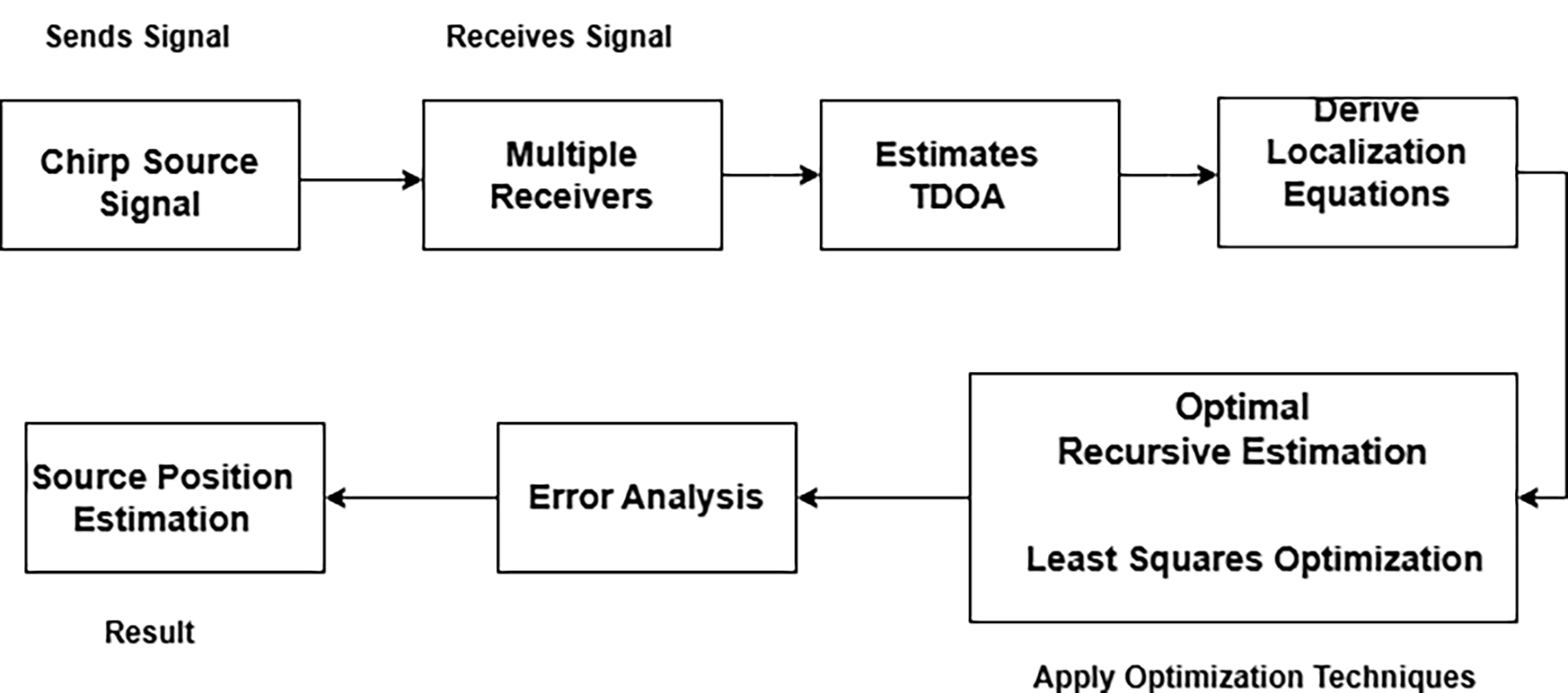
Figure 1 illustrates the methodology for underwater source localisation using TDOA in combination with optimisation techniques. This approach enhances localisation accuracy by compensating for environmental noise and measurement uncertainties. Additionally, the accuracy can be further improved through the use of Kalman filtering and least-squares methods.
Source localisation using TDOA with optimisation techniques.

3. Proposed algorithm, mathematical formulation and comparative discussion
Notation. Let the unknown source position be s = [x, y, z]T and receiver i position be r i = [x i, y i, z i]T. The propagation speed is c. The geometric range is d i(s) = ‖s−r i‖. For a reference receiver i, the model-based TDOA is τ i1(s) = (d i(s) − d 1(s))/c. Measured TDOA values are denoted by τˆi1.
Algorithm overview (integration of KF, EKF, and LS);
-
Step 1. Acquire hydrophone signals and estimate pairwise TDOA via GCC/cross-correlation.
-
Step 2. Initialise source estimate with nonlinear least squares (NLS) using the TDOA measurement model.
-
Step 3. For dynamic scenarios, run KF/EKF prediction using a constant-velocity motion model.
-
Step 4. Update the filter using the TDOA measurement function (EKF uses the Jacobian of τ i1(s)).
-
Step 5. Optionally refine each filtered estimate with a short NLS refinement (1–3 iterations) to reduce residual bias.
-
Step 6. Output position estimate and error statistics.
Flow diagram (textual).
Signals → TDOA extraction → (Init: NLS) → Prediction (KF/EKF) → Update (TDOA residuals) → Optional NLS refinement → Final estimate.
Mathematical analysis. The proposed solution is formulated as a constrained nonlinear least-squares problem. Given M receivers, define the residual vector

The NLS estimator solves
 ${{\rm s*} = {\rm argmin}_{s}\;r{(s)^{T}\;W\;r(s)}},$
where W is a weighting matrix (often W = R −1, R = covariance of the TDOA estimates). This formulation is maximum-likelihood under Gaussian TDOA errors and directly justifies the optimisation component.
For EKF updates, the measurement function is h(s) = [τ 21(s), …, τ M1(s)]T. The Jacobian H = ∂h/∂x evaluated at the predicted state ⓢ– provides a first-order linearisation. For receiver i, the gradient is

Using this Jacobian in the EKF update reduces linearisation error compared with a linear KF measurement model and explains the faster error decay observed in the parametric noise study.
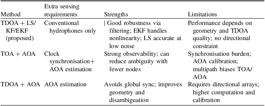
Comparative discussion with hybrid baselines. TOA + AOA and TDOA + AOA reduce geometric dilution by adding directional information, but require either synchronised clocks (TOA) or calibrated array processing (AOA). The proposed framework targets scenarios where only conventional hydrophones are available; it improves robustness via filtering + optimisation without changing the sensing hardware. Section 5 includes a qualitative comparison table; if AOA measurements are available, the same NLS/EKF formulation can be extended by augmenting the residual with AOA terms. Comparison summary is given in Table 1.
Comparison summary.

Table 1 Long description
A table comparing methods for sensing requirements, strengths, and limitations. The table has four rows and four columns. The columns are labeled Method, Extra sensing requirements, Strengths, and Limitations. Row 1: Method, TDOA + LS/KF/EKF (proposed); Extra sensing requirements, Conventional hydrophones only; Strengths, Good robustness via filtering; EKF handles nonlinearity; LS accurate at low noise; Limitations, Performance depends on geometry and TDOA quality; no directional constraint. Row 2: Method, TOA + AOA; Extra sensing requirements, Clock synchronisation + AOA estimation; Strengths, Strong observability; can reduce ambiguity with fewer nodes; Limitations, Synchronisation burden; AOA calibration; multipath biases TOA/AOA. Row 3: Method, TDOA + AOA; Extra sensing requirements, AOA estimation; Strengths, Avoids global sync; improves geometry and disambiguation; Limitations, Requires directional arrays; higher computation and calibration.
4. Simulation results
TDOA-based source localisation using Kalman filter and least-squares optimisation is evaluated with the following initial conditions: receiver positions are fixed and known; sound speed c = 1500 m/s; noise level = 80 dB; signal frequency = 1000 Hz; sampling rate = 10 kHz. First, a static source is considered, followed by a moving source with constant velocity. Three hydrophones are placed at known locations. The estimated source position is illustrated in Figure 2 (LS-based static localisation) and Figure 3 (KF-based static localisation).
Static source localisation using least squares.

Static source localisation using Kalman filter.

In static source localisation using TDOA with least squares and Kalman filter optimisation, the least squares successfully estimated the source position with the lowest possible error when compared with the Kalman filter. Figures 2 and 3 visualise that the least squares is the best for static source localisation. In dynamic source localisation, it was considered that the source moves with a constant velocity and the source location is estimated by considering the noise that is naturally present in the underwater. The results obtained using the Kalman filter will give an idea that in dynamic source localisation by making use of the TDOA, the trajectory of the true source will vary when compared with the estimated source trajectory at the beginning, but will coincide with the true source trajectory as time progresses, as shown in Figure 4 (KF-based trajectory tracking).
Trajectory of the source using Kalman filter.

The localisation error will decrease over time as the estimated source aligns with the true source as shown in Figure 5. Consequently, after the specified duration of 15 seconds, the error will be reduced (Figure 6). With the help of a Kalman filter, the localisation is performed over different noise levels and the results demonstrate that, regardless of the noise, the localisation error decreases over time as the estimated source aligns more closely with the actual source. Figure 7 illustrates the localisation error across different noise levels when using a Kalman filter.
Localisation error over time using Kalman filter.

Trajectory of the source using extended Kalman filter.

Localisation error across different noise levels using Kalman filter.

Figure 7 Long description
The image contains four line graphs, each depicting localization error across different noise levels using Kalman filter. Panel A: The line graph shows localization error for noise level 60 dB. The x-axis represents time in seconds ranging from 0 to 15, and the y-axis represents localization error in meters ranging from 0 to 20. The graph shows a high initial error that decreases over time with minor fluctuations. Panel B: The line graph shows localization error for noise level 80 dB. The x-axis represents time in seconds ranging from 0 to 15, and the y-axis represents localization error in meters ranging from 0 to 20. The graph shows a high initial error that decreases over time with minor fluctuations. Panel C: The line graph shows localization error for noise level 90 dB. The x-axis represents time in seconds ranging from 0 to 15, and the y-axis represents localization error in meters ranging from 0 to 20. The graph shows a high initial error that decreases over time with minor fluctuations. Panel D: The line graph shows localization error for noise level 100 dB. The x-axis represents time in seconds ranging from 0 to 15, and the y-axis represents localization error in meters ranging from 0 to 20. The graph shows a high initial error that decreases over time with minor fluctuations.
It was observed that by using an Extended Kalman Filter (EKF), the accuracy can be achieved more significantly than with Kalman filter. As it considers nonlinearity in the existing localisation, as shown in Figure 6 (EKF error convergence). In the case of the extended Kalman filter, the noise over time decreases more rapidly than with the Kalman filter, as shown in Figure 8, which is also exhibits at different noise levels as shown in Figure 9, which exhibits localisation at different noise levels.
Localisation error over time using extended Kalman filter.

Localisation error across different noise levels using extended Kalman filter.

Figure 9 Long description
The image contains four line graphs, each titled Localization Error Over Time. Each graph has the same structure: the x-axis represents Time in seconds ranging from 0 to 15, and the y-axis represents Error in meters ranging from 0 to 20. Panel A: The line graph shows a sharp initial peak in error around 2 seconds, followed by a rapid decline and smaller fluctuations, stabilizing around 1 meter after 10 seconds. Panel B: The line graph displays a similar pattern with an initial peak around 2 seconds, a rapid decline, and smaller fluctuations, stabilizing around 1 meter after 10 seconds. Panel C: The line graph shows an initial peak around 2 seconds, a rapid decline, and smaller fluctuations, stabilizing around 1 meter after 10 seconds. Panel D: The line graph depicts an initial peak around 2 seconds, a rapid decline, and smaller fluctuations, stabilizing around 1 meter after 10 seconds.
Source localisation using least-squares optimisation estimates the position of a moving source in which the estimated trajectory initially deviates, but later aligns closely with the true path, indicating the effectiveness of the localisation technique used, which is shown in Figure 10. The error increases over time, indicating that noise affects accuracy progressively. The nonlinear trend suggests growing inaccuracies in the localisation algorithm.
Trajectory of the source using least squares.

The localisation error will be increased concerning the noise in the underwater as in the case of least-squares optimisation. Figure 11 visualises the localisation error over different noise levels. Initially, the error will be minimum, but over time for any noise level, the error increases representing the divergence of the estimated source from the true source. The localisation error will be increased over time, as shown in Figure 12. This shows that least-squares optimisation is sensitive to the noise where noisy environments will have a drastic impact on the localisation accuracy.
Localisation error across different noise levels using least squares.

Localisation error over time using least squares.

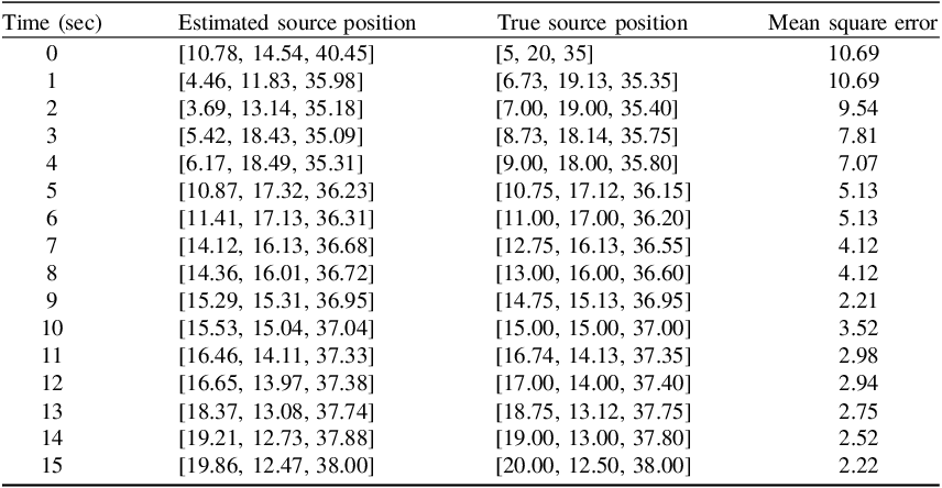
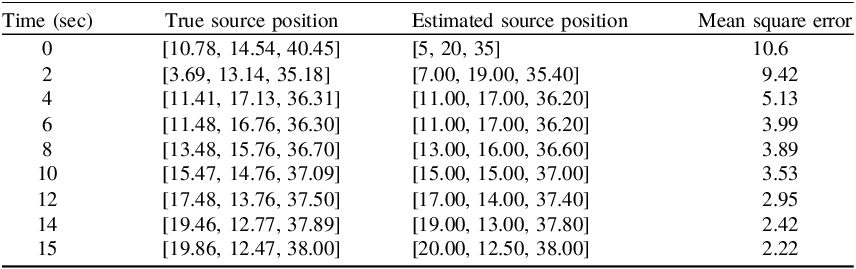
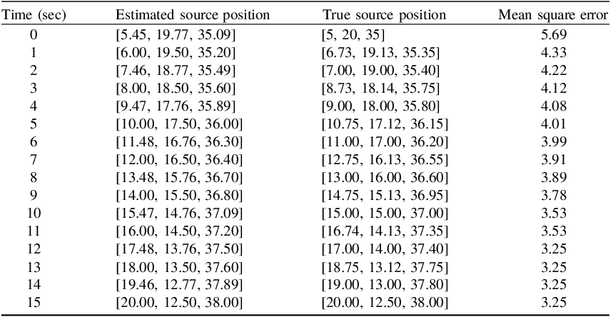
Localisation using the Kalman filter, extended Kalman filter and least squares at a maximum noise level is shown in Tables 2, 3 and 4, respectively. At lower noise levels, the least squares will outperform the Kalman filter optimisation, but as the noise increases, the Kalman filter becomes more accurate than the least squares. The localisation error obtained using the Kalman filter will be reduced over time, but in the case of least squares, the error will remain the same (not much difference over time) As the estimated source position will coincide with the true source position, the error will be reduced. It is to be noted that by using the extended Kalman filtering, the localisation is further reduced as the estimated source position matches with the true source position. Further, the extended Kalman filter is the best option in the case of nonlinear environments as shown in this case.
Localisation using Kalman filter at noise level 100 db.

Table 2 Long description
The table presents data on the localization of a source using the Kalman filter at a noise level of 100 decibels. It includes three columns: Time (sec), Estimated source position, True source position, and Mean square error. The table has 16 rows, each representing data at a specific time point from 0 to 15 seconds. Each row lists the estimated source position, the true source position, and the mean square error at that time point. The estimated and true source positions are given as coordinates in three dimensions. The mean square error values indicate the accuracy of the estimated source position compared to the true source position, with lower values indicating higher accuracy. Notable trends include a general decrease in mean square error over time, suggesting improved accuracy of the estimated source position as time progresses.
Localisation using extended Kalman filter at noise level at 100 db.

Table 3 Long description
A table with five columns and sixteen rows. The columns are labeled Time (sec), true source position, Estimated source position, and Mean square error. The rows present data for time intervals from 0 to 15 seconds. Each row lists the true source position, the estimated source position, and the mean square error for that time interval. The true source position and estimated source position are given as three-dimensional coordinates. The mean square error values decrease over time, indicating improving accuracy of the estimated source position.
Localisation using least squares at noise level 100 db.

Table 4 Long description
The table presents data on estimated source positions, true source positions, and mean square errors over a period of 16 seconds. It has 16 rows and 4 columns. The columns are labeled Time (sec), Estimated source position, true source position, and Mean square error. Each row lists the time in seconds, the estimated source position as a set of three coordinates, the true source position as a set of three coordinates, and the mean square error value. The table shows the progression of these values over time, with the mean square error generally decreasing as time increases.
5. Conclusion
This paper presented an optimisation-based framework for robust underwater acoustic source localisation using TDOA measurements. The framework combines nonlinear least-squares (NLS) positioning with recursive Bayesian tracking (KF) and its nonlinear extension (EKF). The key benefit is that improved robustness is achieved without requiring additional sensing modalities (e.g. AOA arrays) or global time synchronisation.
A parametric analysis was carried out by varying the noise level of the received signals and examining localisation error versus time and versus noise. The results indicate a clear trade-off: (i) LS yields highly accurate estimates for static/low-noise conditions, but becomes sensitive as noise increases; (ii) KF improves robustness for moving sources by exploiting temporal consistency; and (iii) EKF further reduces error and converges faster because it explicitly models the nonlinear TDOA measurement function through Jacobian linearisation.
Compared with hybrid baselines (TOA + AOA, TDOA + AOA), the proposed approach is most suitable when only conventional hydrophones are available, and when system complexity, calibration and cost must be minimised. When AOA measurements are available, the proposed NLS/EKF formulation can be extended by augmenting the measurement vector with bearing residuals to obtain further accuracy gains. Future work will include implementing and benchmarking these hybrid extensions experimentally and studying robustness under sound-speed uncertainty and multipath-dominant channels.