1. Introduction
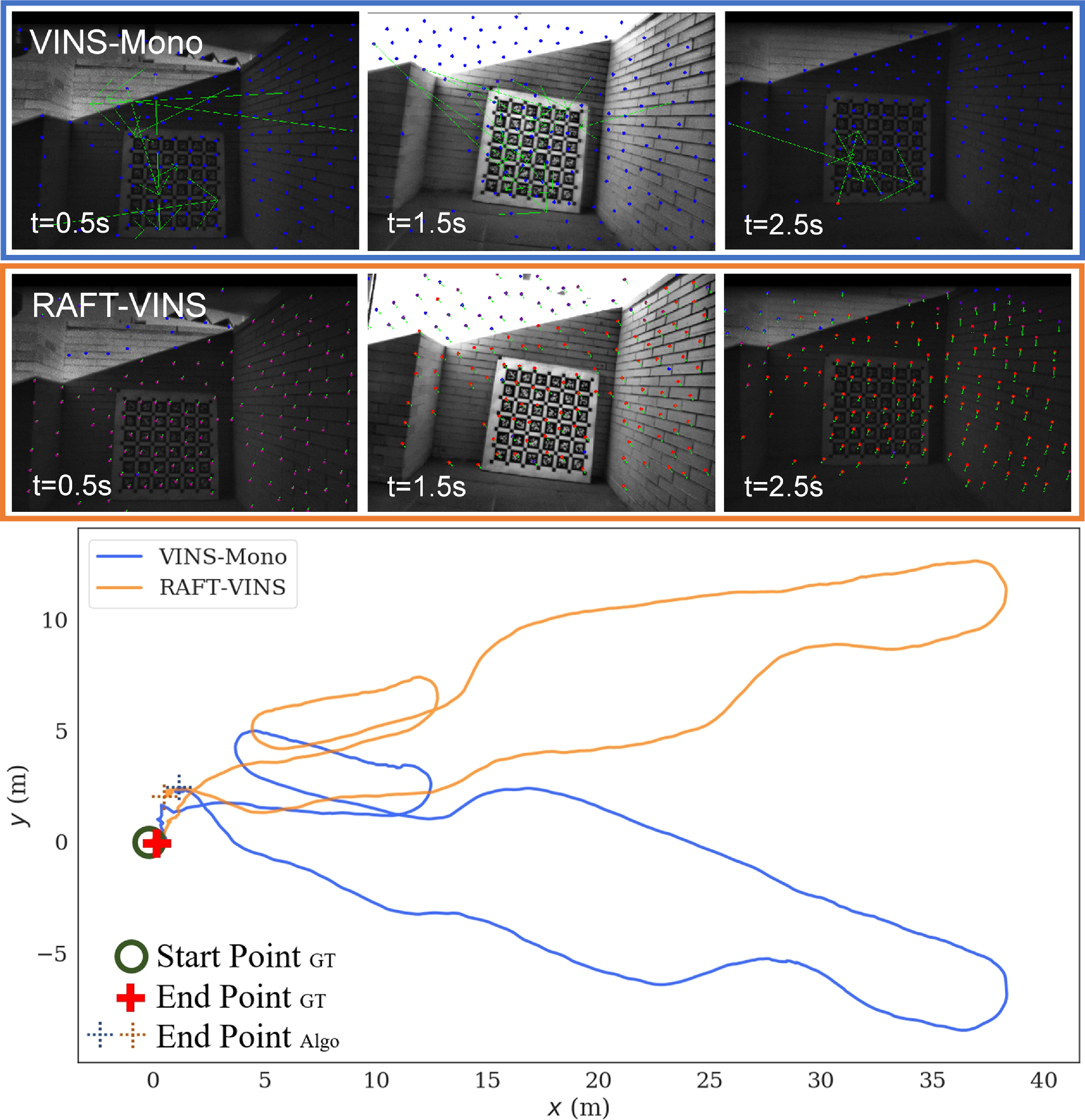
Simultaneous localization and mapping (SLAM) has received widespread attention and application in robot navigation, autonomous driving, and augmented reality. Monocular visual SLAM methods [Reference Forster, Pizzoli and Scaramuzza1–Reference Engel, Koltun and Cremers3] provide a portable and low-cost solution for the six degrees-of-freedom (DoF) pose estimation, and a series of research [Reference Leutenegger, Lynen, Bosse, Siegwart and Furgale4–Reference Yu, Qin, Wang, Wang and Wang6] have further integrated the motion information from the Inertial Measurement Unit (IMU) to enhance their performance. Nevertheless, most of these existing visual-inertial SLAM methods work well only in the environments with sufficient and invariant illumination, while the illumination condition is constantly changing in realistic environments due to the scene transition, dynamic lighting, or onboard illumination for dark environments. Similar to the difficulties encountered in dynamic environments [Reference Yu, Zheng and Ou7–Reference Zhang, Dong, Guo, Ye, Gao, Xiang, Chen and Wu9], dynamic illumination also brings challenges to feature association and consequently reduces the reliability of pose estimation. Ref. [Reference Zuñiga-Noël, Jaenal, Gomez-Ojeda and Gonzalez-Jimenez10] as shown in Figure 1. Therefore, it is necessary to achieve the robust and accurate feature tracking under dynamic illumination conditions to guarantee the performance of the SLAM systems.
In visual SLAM, the most commonly used feature tracking methods include the feature matching and the optical flow tracking. The former one consists of three steps: feature extraction, descriptor computation, and descriptor-based feature matching [Reference Mur-Artal, Montiel and Tardos2], while the latter bypasses descriptor computation and directly calculates the displacements of features. The optical flow tracking method requires less computational complexity and exhibits superior real-time performance in practical applications. Horn and Schunck [Reference Horn and Schunck11] formulated the optical flow estimation problem as the minimization of an energy function, solving for dense optical flow. Lucas Kanade [Reference Lucas and Kanade12] constructed overdetermined equations and solved the sparse optical flow through iterative optimization. However, these traditional methods are based on the assumption of brightness consistency, which makes them unable to achieve reliable feature tracking results in dynamic illumination environments.
Illustration of the trajectory comparison in the two-floor-csc1 sequence. The feature tracking process is shown above, and the green arrows represent the motion of features. In dynamic illumination environments, VINS-Mono experiences drifts due to mismatches, whereas RAFT-VINS remains unaffected with the proposed robust feature tracking.

With the progression of deep learning, numerous optical flow networks [Reference Dosovitskiy, Fischer, Ilg, Hausser, Hazirbas, Golkov, Van Der Smagt, Cremers and Brox13–Reference Teed and Deng17] have emerged to directly estimate optical flow. These deep learning-based methods can overcome the challenge of dynamic illumination, as the convolutional features extracted from RGB images provide advanced information with some degree of illumination invariance. FlowNet [Reference Dosovitskiy, Fischer, Ilg, Hausser, Hazirbas, Golkov, Van Der Smagt, Cremers and Brox13] first utilizes Convolutional Neural Networks for estimating optical flow. It formulates the estimation problem as a supervised regression task and introduces two frameworks, FlowNetS and FlowNetC. Based on the FlowNet, FlowNet2 is proposed in ref. [Reference Ilg, Mayer, Saikia, Keuper, Dosovitskiy and Brox14], which stacks the FlowNetS and FlowNetC networks and achieves comparable accuracy to traditional methods. However, the cascaded structure of the FlowNet2 increases the model parameters, making it challenging to be deployed on practical mobile devices. To deal with this challenge, SpyNet [Reference Ranjan and Black15] and PWC-Net [Reference Sun, Yang, Liu and Kautz16] are designed, introducing coarse-to-fine pyramids to reduce model parameters. By combining with iterative refinement, an equilibrium is attained between precision and parameters. Nevertheless, it is difficult to correct optical flow estimation errors in coarse resolutions. To overcome this issue, RAFT [Reference Teed and Deng17] utilizes a gated recurrent unit module for continuous iterative refinement at high resolutions. Additionally, weight-sharing between iterations allows RAFT to overcome the limitations of iteration counts and achieve remarkable results. The aforementioned learning-based approaches present promising results. However, these networks have not been widely applied to SLAM systems since their computational demands are intolerable for real-time applications.
Recently, a series of studies have focused on the challenging scenarios, such as the scenarios with dynamic objects and the low-texture ones, when considering visual SLAM. Refs. [Reference Yu, Zheng and Ou7, Reference Ding, Pei, Yang and Chen8] focus on dynamic object environments. CPR-SLAM [Reference Yu, Zheng and Ou7] clusters depth images into sub-point clouds and uses their structural invariance and relative relationships to remove dynamic objects. Ding et al. [Reference Ding, Pei, Yang and Chen8] propose a lightweight dynamic SLAM algorithm that combines deep learning object detection with Kalman filters to provide prior information on dynamic objects, followed by geometric techniques to filter out dynamic feature points. Refs. [Reference Pumarola, Vakhitov, Agudo, Sanfeliu and Moreno-Noguer18, Reference Fu, Wang, Yu, Ali, Guo, He and Zhang19] focus on low-texture environments. PL-SLAM [Reference Pumarola, Vakhitov, Agudo, Sanfeliu and Moreno-Noguer18] is based on ORB-SLAM and improves the system’s accuracy in low-texture environments by introducing line features. Fu et al. [Reference Fu, Wang, Yu, Ali, Guo, He and Zhang19] propose PL-VINS, which improves the efficiency of the line feature extraction algorithm and achieves a real-time and high-efficiency point-line visual-inertial SLAM system. Besides the aforementioned two types of challenging scenarios, the ones with dynamic illumination are also common in practice. AirVO [Reference Xu, Hao, Yuan, Wang and Xie20] uses line features and learning-based point features to achieve an illumination-robust stereo visual odometry. However, it lacks the use of IMU information, which causes the system to fail when visual information is limited. Additionally, the learning-based point feature extraction and matching are very time-consuming, which limits their odometry output frequency.
Motivated by the above discussions, we present the RAFT-VINS, a tightly-coupled visual-inertial odometry (VIO) with robust feature association in dynamic illumination environments. It incorporates a lightweight optical flow network capable of real-time inference of dense pixel motion information, which is utilized for accurate feature tracking. As a complement, we develop a moving consistency check strategy that leverages multi-frame reprojection errors to identify and remove feature points with incorrect associations, further improving the accuracy of pose estimation.
The main contributions of this paper are listed as follows:
-
• An efficient and illumination-insensitive visual-inertial odometry, named RAFT-VINS, is proposed, which can provide more accurate real-time 6-DoF pose estimates in dynamic illumination environments when compared with most existing VIO methods.
-
• In the RAFT-VINS, a lightweight optical flow network is designed to significantly reduce the inference time and enhance feature tracking performance. In addition, an outlier points removal strategy based on multi-frame reprojection errors is proposed to further improve the estimation accuracy.
-
• Extensive experiments are conducted to show the proposed system’s competitively accurate and robust pose estimates in dynamic illumination environments.
2. System overview
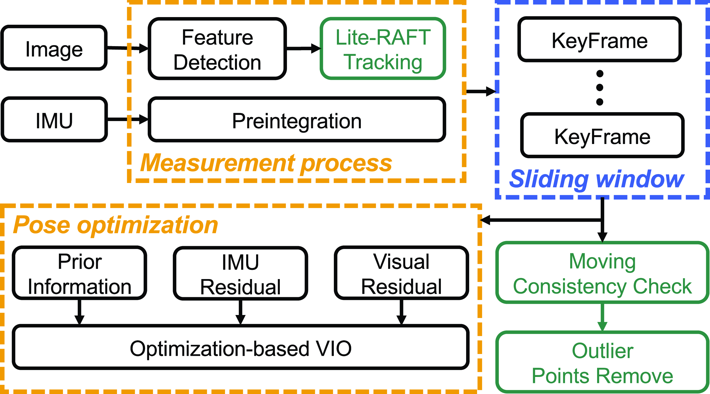
Our algorithm is specifically designed for visual-inertial odometry, making it insensitive to dynamic illumination. It is constructed based on VINS-Mono [Reference Qin, Li and Shen5], with the framework illustrated in Figure 2. In RAFT-VINS, two main threads run in parallel: feature tracking and pose optimization. Additionally, we maintain a fixed-size keyframes sliding window to control the computational complexity of the optimization process. Inputs of the odometry consist of the time-synchronized images and IMU measurements. Color images are employed for feature detection and tracking. IMU measurements between two consecutive image frames are preintegrated for pose optimization [Reference Shen, Michael and Kumar21].
In the feature tracking thread, features are tracked by the proposed Lite-RAFT tracking method and overcome the negative effects of the dynamic illumination. Then, the pose optimization thread tightly fuses the visual and IMU measurement residuals within the sliding window for the pose estimation. Finally, the moving consistency check leverages the optimized pose results to calculate multi-frame reprojection errors and remove outlier points.
The notations employed in this paper are outlined as follows: We denote
 $(\!\cdot\!)^w$
as the world frame,
 $(\!\cdot\!)^b$
as the body frame situated at the IMU frame, and
 $(\!\cdot\!)^c$
as the camera frame. The
 $(\!\cdot\!)^w_{b_k}$
represents the coordinate transformation from the
 $k$
th body frame to the world frame, while
 $(\!\cdot\!)^b_c$
denotes the transformation known as the extrinsic parameters.
The full state vector
 $\mathcal{X}$
to be estimated in the sliding window is defined as
 \begin{align} \mathcal{X} &=[\mathbf{x}_0,\mathbf{x}_1,\ldots \mathbf{x}_n, \lambda _0,\lambda _1,\ldots \lambda _m, \mathbf{q}_c^b, \mathbf{p}_c^b], \nonumber \\ \mathbf{x}_k&=[\mathbf{p}_{b_k}^w, \mathbf{v}_{b_k}^w, \mathbf{q}_{b_k}^w, \mathbf{b}_a, \mathbf{b}_\omega ],\\[6pt]\nonumber \end{align}
where
 $\mathbf{x_k}$
represents the IMU state at the
 $k$
th image capture time.
 $\mathbf{p}_{b_k}^w$
,
 $\mathbf{v}_{b_k}^w$
, and
 $\mathbf{q}_{b_k}^w$
, respectively, denote the position, velocity, and orientation transformation from IMU frame to world frame.
 $\mathbf{q}_c^b$
and
 $\mathbf{p}_c^b$
are the extrinsic parameters between the camera frame and the IMU frame.
 $\mathbf{b}_a$
and
 $\mathbf{b}_\omega$
respectively denote the bias of the accelerometer and gyroscope.
 $\lambda$
is the inverse depth of the feature.
Overview of proposed visual-inertial odometry. The modules we newly designed are highlighted with green blocks.

3. Methodology
In this section, we introduce the details of RAFT-VINS as shown in Figure 2. Firstly, we introduce the IMU preintegration process. Then, the lightweight optical flow network and moving consistency check strategy are designed for feature tracking and the removal of outlier feature points, respectively. Finally, we employ a tightly-coupled nonlinear optimization framework for efficient and highly accurate pose estimation.
3.1. IMU preintegration
The raw measurements of an IMU primarily consist of the three-axis acceleration
 $\hat {\mathbf{a}}_t$
and angular velocity
 $\hat {\boldsymbol{\omega }}_t$
, both of which are in the IMU body frame. These measurements are influenced by
 $\mathbf{b}_a$
,
 $\mathbf{b}_{\omega _t}$
, and additive Gaussian white noise. Short-term IMU measurements can be used for pose prediction, and the IMU continuous-time kinematics integration model is given as follows:
 \begin{align} \mathbf{p}_{b_{k+1}}^w &= \mathbf{p}_{b_{k}}^w + \mathbf{v}_{b_k}^w \delta t + \iint _{t_k}^{t_{k+1}} [\mathbf{R}_t^{w}(\hat {\mathbf{a}}_t-\mathbf{b}_{a_t}) - \mathbf{g}^w]dt^2, \nonumber \\ \mathbf{v}_{b_{k+1}}^w &= \mathbf{v}_{b_{k}}^w + \int _{t_k}^{t_{k+1}} [\mathbf{R }_t^{w}(\hat {\mathbf{a}}_t-\mathbf{b}_{a_t}) - \mathbf{g}^w]dt, \nonumber \\ \mathbf{q}_{b_{k+1}}^w &= \mathbf{q}_{b_{k}}^w \otimes \int _{t_k}^{t_{k+1}} \frac {1}{2} \Omega (\hat {\boldsymbol{\omega }}_t - \mathbf{b}_{\omega _t})\mathbf{q}_t^{b_k}dt, \end{align}
where
 \begin{equation} \boldsymbol{\Omega }(\boldsymbol{\omega }) = \begin{bmatrix} -[\boldsymbol{\omega }]_\times & \boldsymbol{\omega } \\ -\boldsymbol{\omega }^T & 0 \end{bmatrix}, \quad [\boldsymbol{\omega }]_\times = \begin{bmatrix} 0 & -\omega _z & \omega _y \\ \omega _z & 0 & -\omega _x \\ -\omega _y & \omega _x & 0 \end{bmatrix}. \end{equation}
In the back-end optimization, the estimation of state vector
 $\mathcal{X}$
is adjusted to minimize the IMU and visual measurement residuals. It is evident from (2) that changes in the state variables necessitate the repropagation of the integral terms. To avoid this, we apply preintegration [Reference Shen, Michael and Kumar21] to all IMU measurements between consecutive image frames to estimate their incremental motion. Specifically, by applying
 $R_w^{b_k}$
to both sides of (2), we decouple the integral term on the right side from the state variables, with the preintegration terms detailed as follows:
 \begin{align} \mathbf{\alpha } _{b_{k+1}}^{b_k} &= \iint _{t_k}^{t_{k+1}} \mathbf{R}_t^{b_k}(\hat {\mathbf{a}}_t-\mathbf{b}_{a_t})dt^2, \nonumber \\ \mathbf{\beta } _{b_{k+1}}^{b_k} &= \int _{t_k}^{t_{k+1}} \mathbf{R}_t^{b_k}(\hat {\mathbf{a}}_t-\mathbf{b}_{a_t})dt, \nonumber \\ \mathbf{\gamma } _{b_{k+1}}^{b_k} &= \int _{t_k}^{t_{k+1}} \frac {1}{2} \mathbf{\Omega }(\hat {\boldsymbol{\omega }}_t-\mathbf{b}_{\omega _t}) \mathbf{\gamma } _{t}^{b_k} dt^2. \end{align}
3.2. Lite-RAFT feature tracking
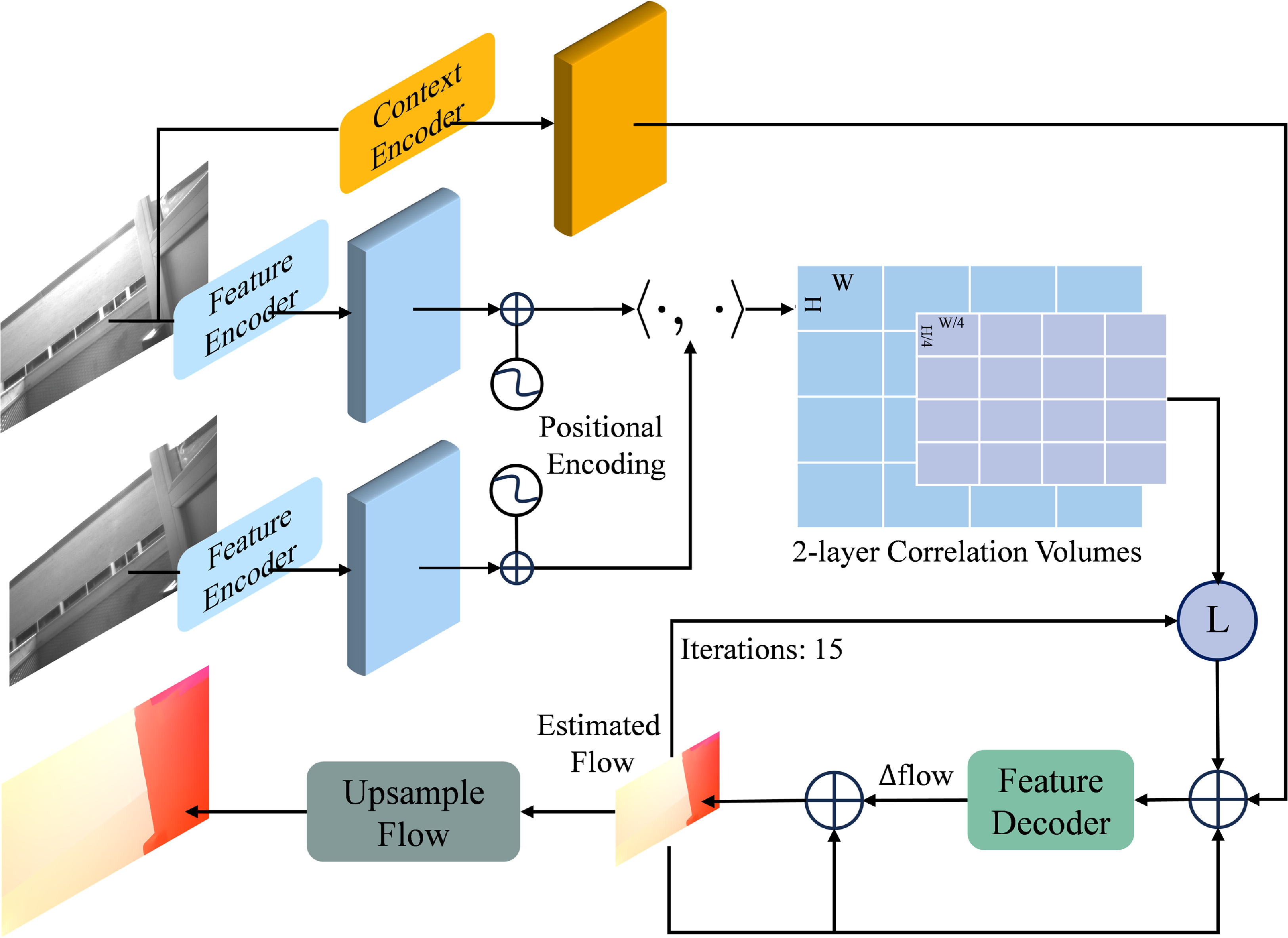
Feature association in dynamic illumination environments is challenging. To mitigate sensitivity to these variations, we design the Lite-RAFT, a lightweight deep network for optical flow estimation, inspired by the RAFT [Reference Teed and Deng17] and ThermalRAFT [Reference Jiang, Chen, Dai, Gao and Zhang22]. Due to the lightweight design, the proposed network can achieve real-time operations within the SLAM system. It comprises three primary components, as shown in Figure 3, including the feature encoder, the correlation volumes, and the feature decoder.
Structure of the proposed Lite-RAFT.

We employ a weight-sharing feature encoder to extract high-dimensional features from the input image pairs, producing feature maps
 $F_1, F_2\in \mathbb{R} ^{H\times W\times D}$
, where
 $H$
,
 $W$
, and
 $D$
denote height, width, and feature dimension, respectively. These extracted features are then added with positional encoding [Reference Carion, Massa, Synnaeve, Usunier, Kirillov and Zagoruyko23], allowing for the consideration of both feature similarity and their spatial distance in subsequent similarity calculations. Additionally, a separate context network with the identical structure as the feature encoder processes the first image to produce a context map, which is used as the input for the feature decoder.
For the two-layer correlation volumes, the first layer with dimension
 $H\times W\times H\times W$
is constructed by taking the dot product between every pair of feature vectors, quantifying the visual similarity of two feature maps. The second layer is obtained by downsampling the first layer. To be specific, the last two dimensions of the first layer are pooled using a kernel with the size of 4 and an equivalent stride, then the second layer with dimension
 $H\times W\times H/4\times W/4$
is obtained. This two-layer correlation volumes we constructed can maintain sensitivity to both large and small displacements. At the same time, it reduces the amount of computation and memory consumption compared to the original RAFT. Note that the lookup radius for the search of correlation information in the correlation volumes is always 4.
The feature decoder estimates the residual flow iteratively, starting with an initial flow set to zero. The context map, previously estimated flow, and indexed correlation volumes are concatenated as the input of the feature decoder. Then, the input passes through four convolutional layers and the residual flow
 $\Delta {\mathbf{f}}$
is obtained as the update term. This term is added to the current flow, which will be fed into the next iteration. Following multiple iterations, the estimated flow undergoes upsampling to match the resolution of the original image using a mask network.
Introducing the aforementioned three components results in a slight reduction in accuracy for Lite-RAFT compared to the original RAFT model. However, it yields a significant improvement in inference speed. By choosing proper number of iterations for the feature decoder, the balance between the accuracy and computational cost can be improved.
The designed Lite-RAFT is trained using an RTX 4070 GPU. To be specific, we pretrain the network on the FlyingChairs dataset [Reference Dosovitskiy, Fischer, Ilg, Hausser, Hazirbas, Golkov, Van Der Smagt, Cremers and Brox13] for 120k iterations with a batch size of 8, and train for 120k iterations on the FlyingThings3D dataset [Reference Mayer, Ilg, Hausser, Fischer, Cremers, Dosovitskiy and Brox24] with a batch size of 5. We then finetune on the Sintel dataset [Reference Butler, Wulff, Stanley and Black25] for another 120k iterations. The pretraining process improves the convergence of the training process of the Lite-RAFT. During the training, we supervise our network using the loss introduced in RAFT [Reference Teed and Deng17], which is given as
 \begin{equation} L = \sum _{i=1}^{N}\gamma ^{N-i}\left \| \mathbf{f}_{\text{true}} - \mathbf{f}_i \right \| _1, \end{equation}
where
 $\mathbf{f}_{\text{true}}$
denotes the ground truth flow and
 $\mathbf{f}_i$
represents the estimated flow at the
 $i$
th iteration. The weight factor is set to
 $\gamma = 0.8$
, implying that the optical flows obtained in the later iterations have higher weights in the overall loss function.
Since the proposed Lite-RAFT can provide efficient and accurate dense optical flow estimation of every integer pixel under dynamic illumination conditions, we employ bilinear interpolation to derive displacement information for tracking existing non-integer features. Furthermore, if the count of features within the field of view falls below a preset threshold during the tracking process, we detect the Shi-Tomas corners [Reference Shi and Tomasi26] and set a minimum separation of corners to ensure a uniform distribution.
3.3. Moving consistency check
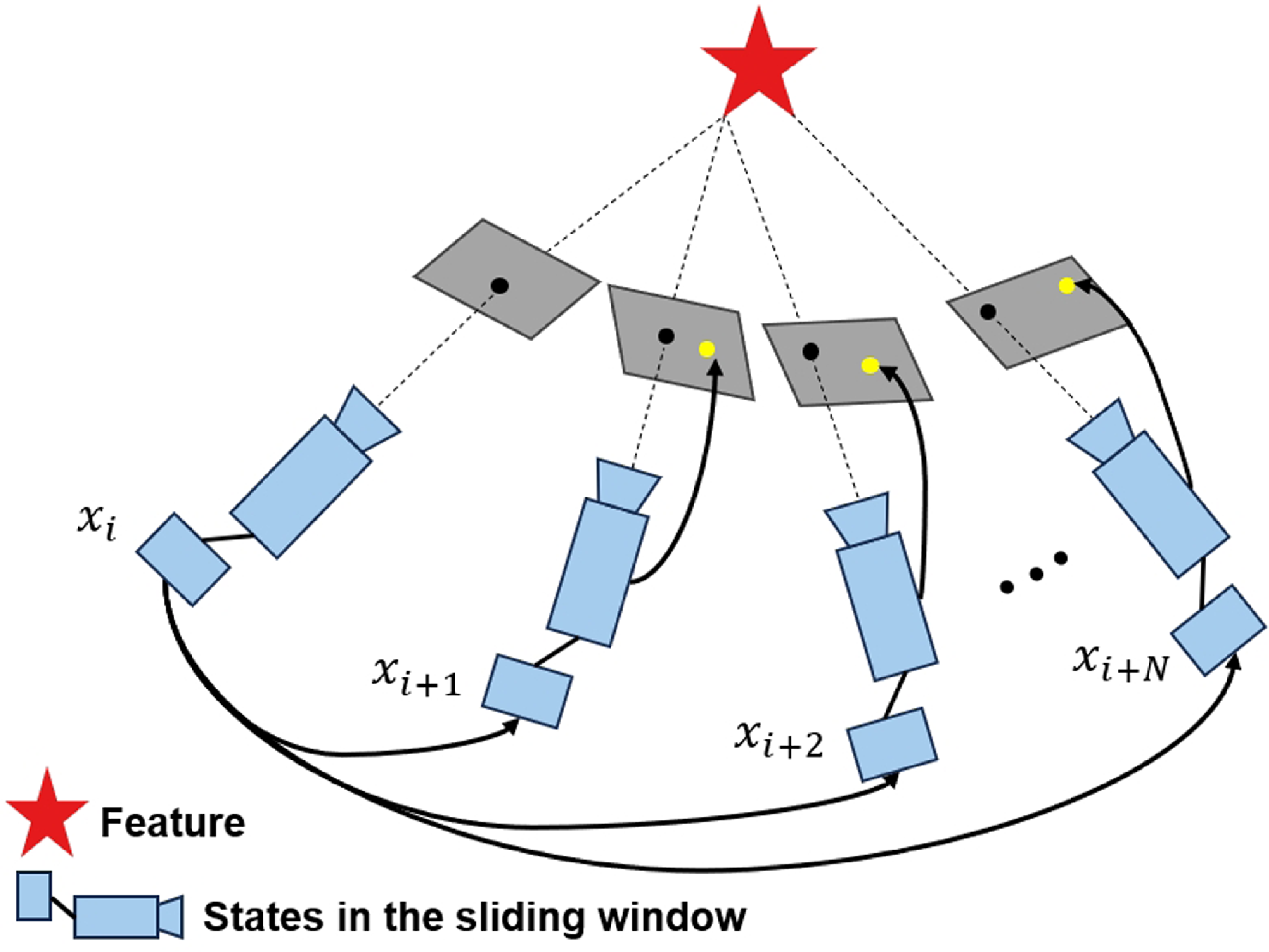
Although the feature tracking performance is significantly improved via using the Lite-RAFT, the tracking errors still exist in certain cases, such as image noise or optical flow prediction inaccuracies in dynamic illumination scenarios. To tackle these issues, we design a moving consistency check strategy within the RAFT-VINS, leveraging the optimized poses within the sliding window to calculate multi-frame reprojection errors. The process to obtain the reprojection errors is illustrated in Figure 4. Considering the
 $k$
th feature, which is initially observed in the
 $i$
th frame and contained in the subsequent
 $n-1$
frames in the sliding windows, we reproject the first observation onto other frames, and the reprojection error is defined as
 \begin{align} r_{k} =\frac {1}{n-1} \sum _{j\ne i} \left \| \hat {\bar {P}}^{c_j}_k -\frac {P_k^{c_j}}{[P_k^{c_j}]_z} \right \| _2, \end{align}
where
 \begin{align*} P_k^{c_j} = T_{b}^{c}T_{w}^{b_j}T_{b_i}^{w}T_{c}^{b}\frac {\hat {\bar {P}}^{c_i}_k}{\lambda }. \end{align*}
 $\lambda$
is the inverse depth of the
 $k$
th feature.
 $\hat {\bar {P}}^{c_i}_k$
and
 $\hat {\bar {P}}^{c_j}_k$
denote the observed normalized coordinates of the
 $k$
th feature in the
 $i$
th and
 $j$
th camera frame, respectively.
 $T_{c}^{b}$
is the extrinsic parameter that represents the transformation from the camera frame to body frame.
 $T_{b_i}^{w}$
and
 $T_{w}^{b_j}$
represent the inverse transformation matrices between the body frame and world frame at
 $i$
th and
 $j$
th frame, respectively. When the residual
 $r_k$
is over a preset threshold, the
 $k$
th feature is considered as an outlier point and removed from the VIO system.
Illustration of the moving consistency check strategy. The red pentagon represents a feature, which is first observed in the
 $i$
th frame. The black arrow represents the projection process, the yellow points are the projected results, and the black points are the actual observations of the landmark in corresponding image frame.

3.4. Tightly-coupled VIO
A tightly-coupled optimization-based framework is used to estimate the state vector
 $\mathcal{X}$
by fusing IMU and visual measurements and minimizing total residuals. The overall objective function for the joint optimization is given as follows:
 \begin{equation} \underset {\mathcal{X}}{\textrm{min}} \left \{ \sum || e_{\mathcal{B}} (\mathcal{X})||^2_{\Sigma _b} + \sum \rho || e_{\mathcal{C}}(\mathcal{X})||^2_{\Sigma _c} + \left \|I_p(\mathcal{X}) \right \|^2 \right \}, \end{equation}
where
 $e_{\mathcal{B}}$
is the IMU residual. With the IMU preintegration introduced in Section 3.1, we can define the IMU residual between two body frames
 $b_k$
and
 $b_{k+1}$
as follows:
 \begin{align} e_{\mathcal{B}} = \begin{bmatrix} \mathbf{R}_w^{b_k}(\mathbf{p}_{b_{k+1}}^w-\mathbf{p}_{b_{k}}^w - \mathbf{v}_{b_{k}}^w t - \mathbf{g}^w t^2 ) - \mathbf{\alpha } _{b_{k+1}}^{b_k} \\[8pt] \mathbf{R}_w^{b_k}(\mathbf{v}_{b_{k+1}}^w-\mathbf{v}_{b_{k}}^w - \mathbf{g}^w \delta t ) - \mathbf{\beta } _{b_{k+1}}^{b_k} \\[8pt] 2\left [ \mathbf{q}_w^{b_k} \otimes \mathbf{q}_{b_{k+1}}^w \otimes (\mathbf{\gamma } _{b_{k+1}}^{b_k})^{-1} \right ]_{xyz} \\[8pt] b_{a_{b_{k+1}}} - b_{a_{b_{k}}} \\[8pt] b_{g_{b_{k+1}}} - b_{g_{b_{k+1}}} \end{bmatrix}, \end{align}
where
 $t$
is the time interval between two consecutive image frames.
 $[\stackrel{{}_{\circ}}{{\textrm{u}}}]_{xyz}$
represents the vector part of the quaternion.
 $e_{\mathcal{C}}$
is the visual measurement residuals, its calculation process is the same as the projection process in Section 3.3.
 $\Sigma _b$
and
 $\Sigma _c$
are the corresponding covariance matrices. We invert covariance matrices to obtain the corresponding information matrices, which are then used to characterize uncertainty and are multiplied by the residuals.
 $I_p$
is the prior information generated during the marginalization process. For more details about
 $e_{\mathcal{B}}$
and
 $I_p$
, please refer to ref. [Reference Qin, Li and Shen5].
 $\rho$
denotes the Huber loss function [Reference Huber27] and is defined as
 \begin{equation} \rho (s) = \begin{cases} s, & s \leq 1; \\ 2\sqrt {s} - 1, & s \gt 1. \end{cases} \end{equation}
This loss function is utilized to effectively suppress large residuals caused by incorrect feature associations, without overly suppressing them, while maintaining a balanced influence on the reprojection error. Equation (7) fundamentally represents a nonlinear least-squares problem, and the Ceres Solver [Reference Agarwal and Mierle28] is employed for its iterative solution.
4. Experiments
In this section, both qualitative and quantitative experiments are conducted to validate the performance of the Lite-RAFT, moving consistency check module, and the whole VIO system RAFT-VINS, especially in the scenarios with dynamic illumination. First, we focus on the real-time performance of the optical flow network and compare it with existing ones. Second, we select some consecutive frames from the UMA-VI dataset [Reference Zuñiga-Noël, Jaenal, Gomez-Ojeda and Gonzalez-Jimenez10] with dynamic illumination conditions to show the robustness of the Lite-RAFT feature tracking method. In addition, we conduct a separate verification on the moving consistency check module. Finally, we conduct several experiments on public datasets and perform realworld deployment tests to validate the effectiveness and accuracy of the whole RAFTVINS.
4.1. Real-time performance of optical flow networks
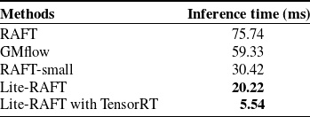
To validate the real-time performance of proposed Lite-RAFT, we compare it with other optical flow networks in the inference time, including the GMflow [Reference Xu, Zhang, Cai, Rezatofighi and Tao29], RAFT [Reference Teed and Deng17], and RAFT-small [Reference Teed and Deng17]. We conduct the experiments on an RTX 4070 GPU, using input image sequences with a resolution of 1440 x 440 pixels. Moreover, the iteration count is set to 15 for both Lite-RAFT and RAFT. Table I shows the average inference time of various networks for 100 runs, and the network Lite-RAFT we design demonstrates a remarkable reduction in time. To be specific, the average inference time of the Lite-RAFT is with improvements of
 $73\%$
,
 $66\%$
, and
 $34\%$
when compared to RAFT, GMFlow, and RAFT-Small, respectively. To further reduce the inference time of the Lite-RAFT and integrate it into VIO systems seamlessly, we implement the network using LibTorch and accelerate it with TensorRT. The combination of these two technologies ensures that the Lite-RAFT operates with high efficiency, guaranteeing the real-time performance of the entire VIO system.
4.2. Feature tracking performance
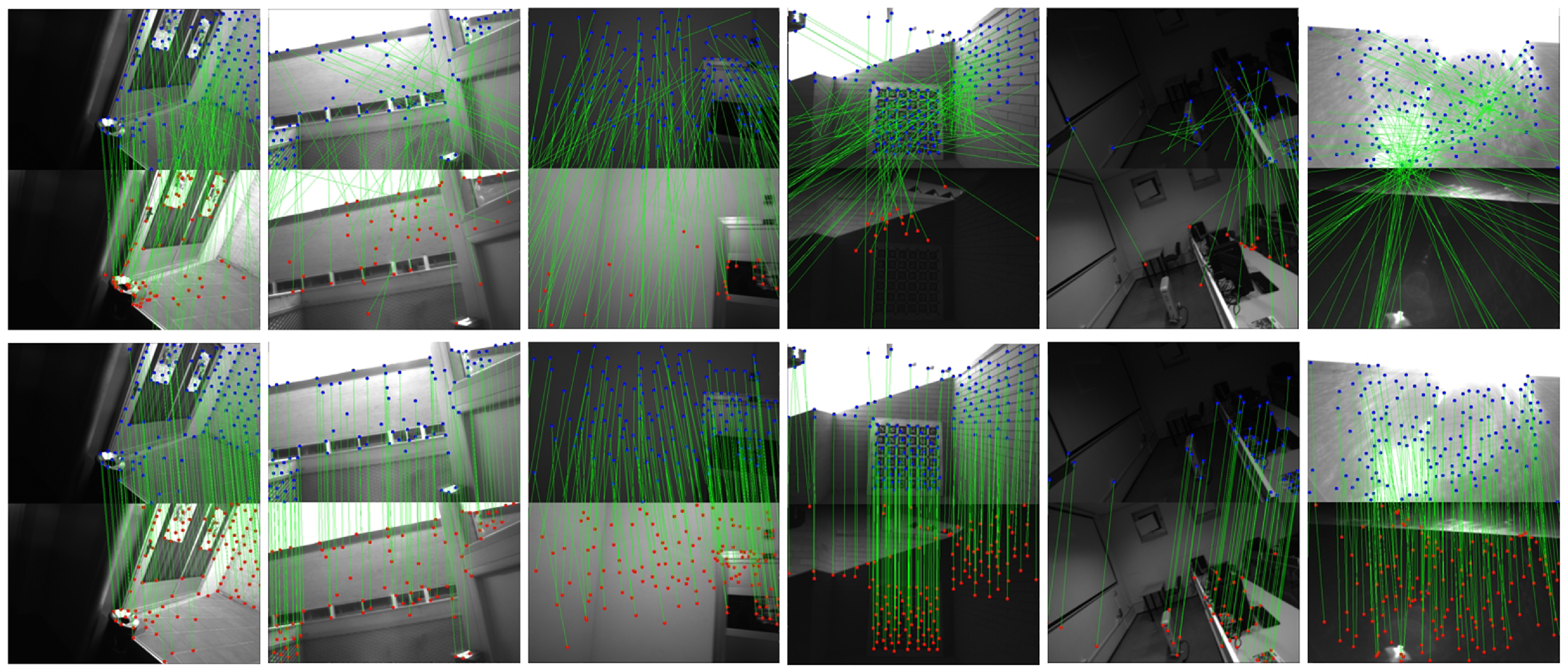
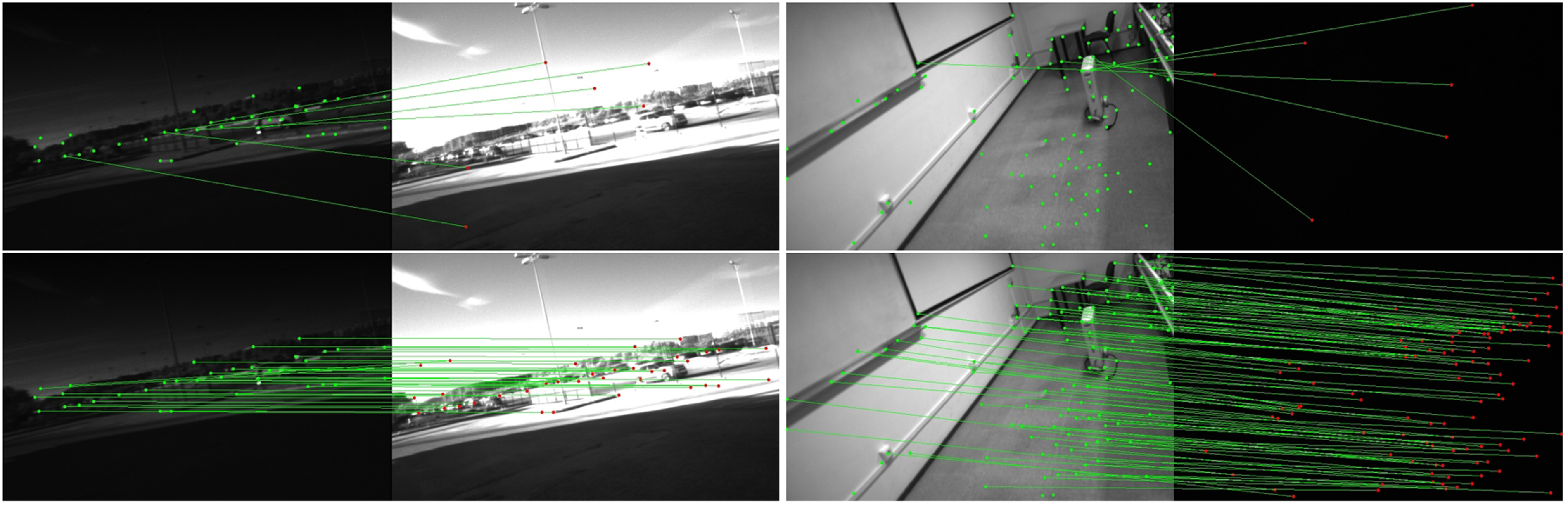
To verify the feature tracking performance of the proposed Lite-RAFT in dynamic illumination environments, we conduct a feature tracking experiment on the image frames chosen from UMA-VI dataset [Reference Zuñiga-Noël, Jaenal, Gomez-Ojeda and Gonzalez-Jimenez10], including indoor scenes and outdoor scenes. These frames involve natural illumination changes and artificial lighting changes, breaking the brightness consistency assumption. Indoor scenes exhibit a wide brightness range with rapid transition speed, while outdoor scenes show a narrower brightness range with slower transition speed. In the experiment, we utilize both the Lite-RAFT tracker and the Kanade-Lucas-Tomasi (KLT) tracker [Reference Lucas and Kanade12] for the feature tracking. The tracking results are depicted in Figure 5, in which the top row exhibits the tracking results of the KLT tracker, while the bottom row exhibits the results of our Lite-RAFT tracking method. The green lines connect the associated features in consecutive frames. It is evident that when there is a change in illumination, the Lite-RAFT tracking method can achieve the feature tracking task accurately, while the KLT tracker produces a significant number of feature mismatches and substantial feature tracking losses. Additionally, we evaluate our method under extreme illumination scenes selected from the UMA-VI dataset, including camera overexposure and sudden environmental darkening. The feature tracking results are shown in Figure 6 demonstrate that our method remains robust and adaptable even in highly dynamic illumination environments.
The average inference time comparison.

Feature tracking performance comparison of the KLT tracker (top row) and the Lite-RAFT tracker (Bottom row).

Feature tracking performance comparison of the KLT tracker (top row) and the Lite-RAFT tracker (bottom row). The left column corresponding to camera overexposure and the right column corresponding to sudden darkness.

4.3. Moving consistency check performance
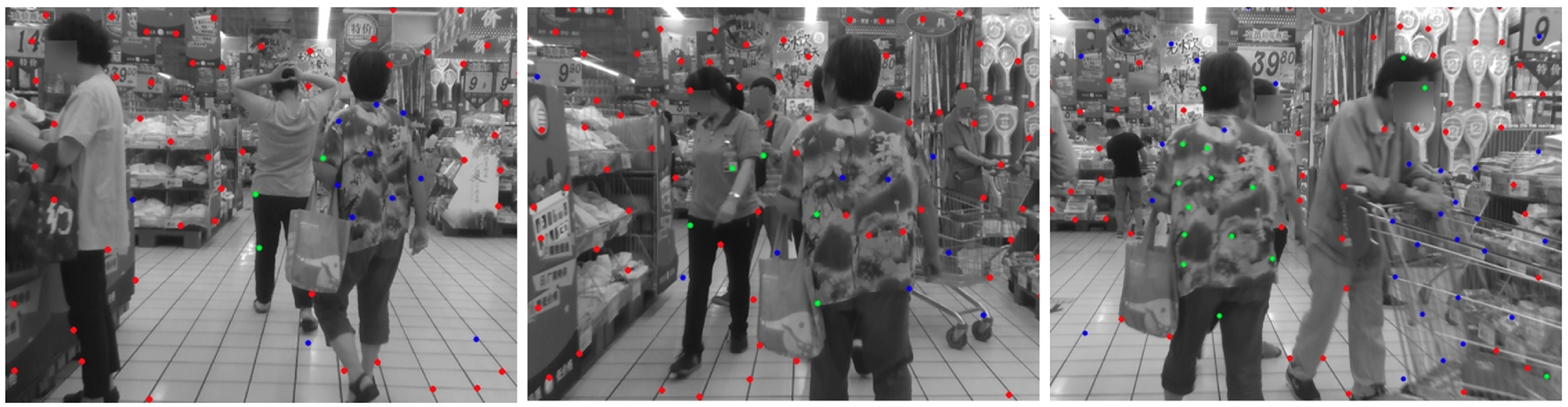
To validate the effectiveness of our moving consistency check module, we compare our approach with the epipolar constraint method utilized in VINS-Mono. Specifically, we select the market sequence from the OpenLORIS dataset [Reference Shi, Li, Zhao, Tian, Tian, Long, Zhu, Song, Qiao, Song, Guo, Wang, Zhang, Qin, Yang, Wang, Chan and She30], which contains a large number of dynamic objects in the scene and provides both image and IMU data. Please note that dynamic objects are introduced to simulate mismatched points for validating the effectiveness of the proposed moving consistency check module. However, removing dynamic objects is not the primary focus of this work. The result of removed outliers is shown in Figure 7. The red points represent the stable tracking points, the green points are outliers identified by the epipolar constraint-based outlier removal strategy in VINS-Mono, and the blue points are the outliers detected by our method. Note that we first perform outlier removal using the epipolar constraint method to identify and remove dynamic points, and then apply our method to identify and remove the remaining dynamic points. Therefore, our method identifies outliers that the epipolar constraint method does not detect.
It can be observed that although the epipolar constraint can effectively remove some dynamic points, it is insufficient in scenarios with numerous dynamic objects, since it only relies on constraints between consecutive images. In contrast, our method makes full use of more accurate multi-frame poses, which enables the effective removal of more dynamic points, thereby improving the system’s localization accuracy.
4.4. Full system evaluation
In this subsection, we conduct experiments on both public datasets and real-world scenarios to comprehensively evaluate the overall performance of RAFT-VINS. In these experiments, we compare RAFT-VINS with the state-of-the-art baseline systems, including VINS-Mono [Reference Qin, Li and Shen5], PL-VINS [Reference Fu, Wang, Yu, Ali, Guo, He and Zhang19], ORB-SLAM3 [Reference Campos, Elvira, Rodríguez, Montiel and Tardós31], AirVO [Reference Xu, Hao, Yuan, Wang and Xie20], and DROID-SLAM [Reference Teed and Deng32], assessing their pose estimation accuracy under dynamic illumination conditions. PL-VINS is an extension of VINS-Mono with the addition of line features. AirVO is an illumination-robust stereo point-line odometry that utilizes deep learning for feature extraction and matching, and DROID-SLAM is an end-to-end (E2E) method based on RAFT. We use the open-source Python package EVO for evaluation to calculate the root mean square error of the Absolute Trajectory Error, and the loop closure detection for all tested methods has been disabled.
4.4.1 Evaluation in UMA-VI Dataset
We conduct the experiments in the UMA Visual-Inertial dataset [Reference Zuñiga-Noël, Jaenal, Gomez-Ojeda and Gonzalez-Jimenez10], which comprises various scenarios with dynamic illumination as shown in Figure 5. This dataset was acquired with a custom handheld visual-inertial unit that integrates a stereo camera (BB2-08S2C-25, 12.5 Hz), two mono cameras (uEye UI-1226LE-M, 25 Hz), and a synchronized Inertial Measurement Unit (Xsens MTi-28A53G35 250 Hz). For our evaluation, we exclusively utilize images captured by the left monocular camera along with data from the IMU. For AirVO, we use stereo images, whereas for DROID-SLAM, only monocular images are used.
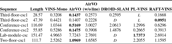
Translational error (root mean square error) comparison in UMA-VI dataset.
 $L$
indicates tracking loss occurred, and
 $D$
indicates significant drift. AirVO (w/o line) refers to the AirVO version without line features.

The outlier detection results. Red points represent stable tracked feature points, green points are outliers detected using the epipolar constraint, and blue points are outliers detected by the motion consistency check module.

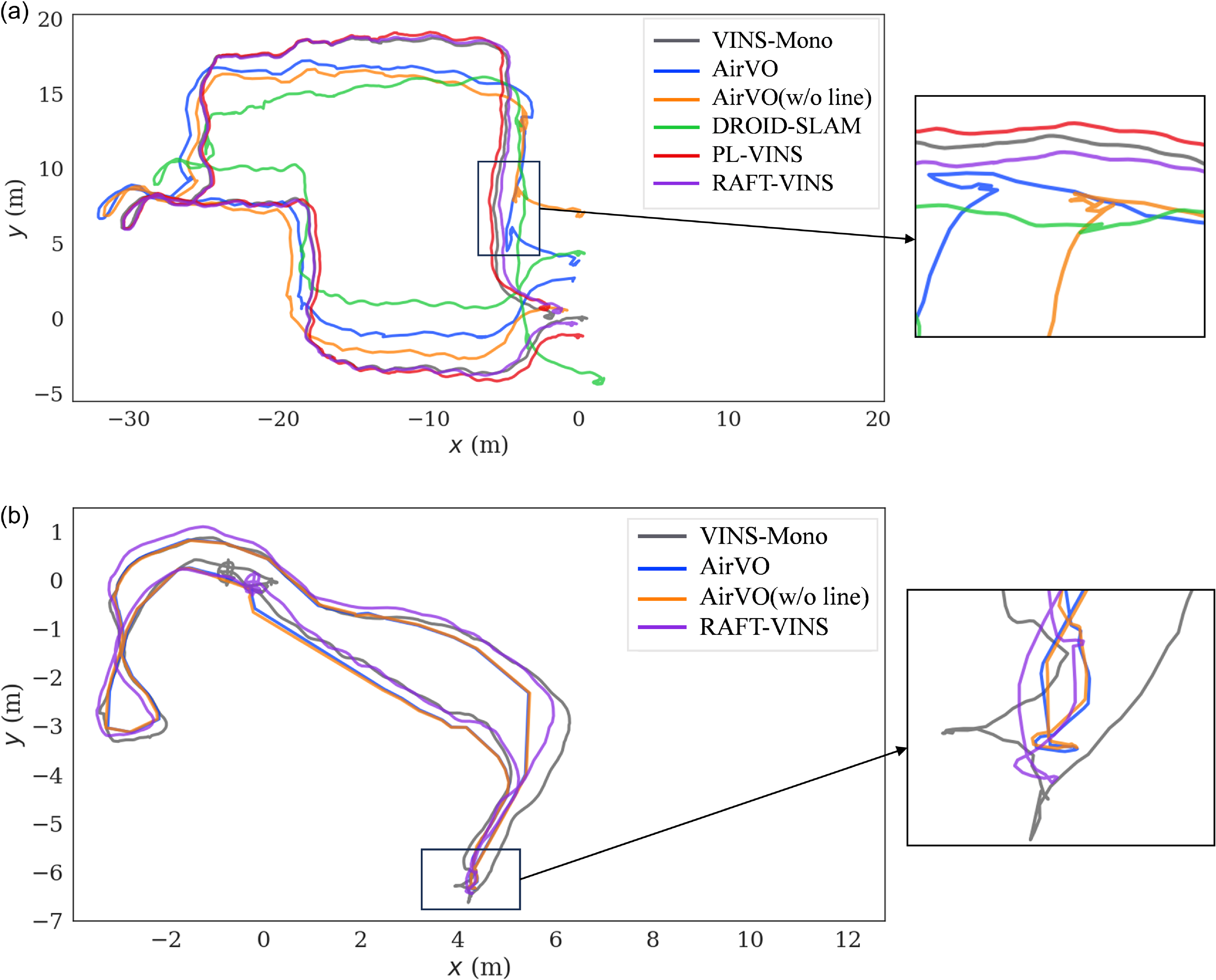
The translation error is shown in Table II. Note that in the UMA-VI dataset, ORB-SLAM3 fails to provide complete trajectory estimates, primarily due to the challenges of extracting and matching ORB features under dynamic illumination conditions. Thus, it is not included in the table. As shown in the table, for all sequences, our method outperforms VINS-Mono, since our Lite-RAFT provides more stable feature tracking. In the absence of line features, our method outperforms AirVO, which improves localization accuracy by using line features. However, AirVO experiences significant drift in the lab-module-csc sequence due to strong dynamic illumination, demonstrating that our method offers better stability in dynamic illumination environments. Due to the inclusion of line features, PL-VINS outperforms our method in two sequences, but underperforms in others, even resulting in tracking loss. RAFT-VINS outperforms DROID-SLAM in all sequences. Additionally, DROID-SLAM performs poorly in longer sequences, especially those containing both indoor and outdoor scenes, where drift tends to occur. The estimated trajectories compare in sequences conference-csc1 and third-floor-csc2 are shown in Figure 8.
Translational error (root mean square error) comparison in EUROC dataset. AirVO (w/o line) refers to the AirVO version without line features.

Comparison of estimated trajectories in sequences conference-csc1 and third-floor-csc2, respectively.

4.4.2 Evaluation in Euroc Dataset
To verify the generality and scalability of our RAFT-VINS, we also conduct tests on the Euroc dataset [Reference Burri, Nikolic, Gohl, Schneider, Rehder, Omari, Achtelik and Siegwart33], which was collected onboard a micro-aerial vehicle. The Euroc dataset is a general scene dataset that does not include illumination changes. We select several typical sequences, including rapid rotations. For each system, we use the same settings as those used during the evaluation with the UMA-VI dataset. The results of various algorithms are shown in Table III.
Among these sequences, ORB-SLAM3 produces the lowest translation error. DROID-SLAM also performs well, though drift is observed in the V2_03_difficult sequence. VINS-Mono and AirVO yield similar results, and our method is comparable to them. However, RAFT-VINS performed poorly in the MH_01_easy and MH_05_difficult sequence, due to the following two factors. First, the EUROC dataset does not involve variations in illumination. In this case, both ORB-based feature matching and KLT-based optical flow tracking perform excellently. Second, in order to improve the real-time performance of Lite-RAFT for feature tracking, we sacrifice some accuracy, which leads to a lower tracking performance in general scenes compared to traditional methods. Therefore, the final evaluation results of translation error are worse than other methods. Nevertheless, our method is generality and scalability to normal scenarios. In addition, it achieves higher localization accuracy in the environments with dynamic illumination, as shown in Table II.
4.4.3 Evaluation in real world
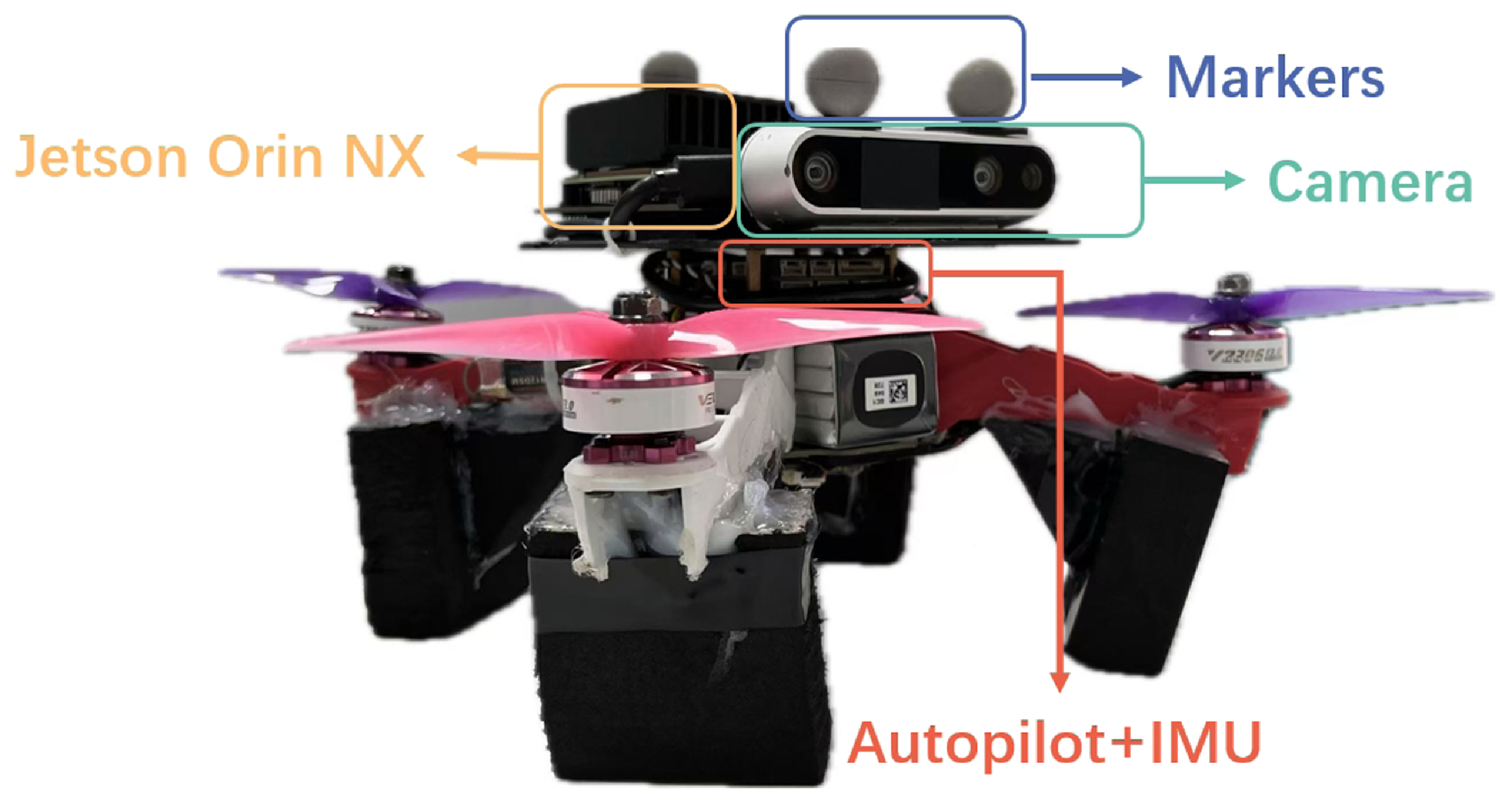
An experiment in the real world is conducted to further evaluate the performance of the RAFT-VINS. In this experiment, we use a quadcopter as shown in the Figure 9 for testing, with all evaluated algorithms deployed on an onboard Jetson ORIN NX 16G computing platform, which provides real-time odometry pose estimation results. Image data are provided by a camera (Intel D435i, 30 Hz), and motion information is provided by an IMU (BMI055, 200 Hz). In Test 1, the quadcopter flies three times around a circle with a radius of 1.8 m. The average flight speed is 2.14 m/s with a maximum speed of 4.08 m/s, and the total flight distance is 46.58 m. In Test 2, the quadcopter flies two times around a figure-eight trail. The average flight speed is 2.06 m/s with a maximum speed of 5.66 m/s, and the total flight distance is 49.16 m. During the flight, dynamic illumination was produced by manually controlling the lights, similar to the indoor sequences in the UMA-VI dataset, with a wide brightness range and rapid transitions. The ground truth of these two flight trajectories is obtained using a motion capture system.
Time consumption statistics for each module of the system (ms).

A quadcopter equipped with a camera, an autopilot with IMU, markers, and an onboard computer.

We deploy all algorithms onto the Jetson ORIN NX platform and conduct a time analysis. We compare the execution time of each module belonging to RAFT-VINS, VINS-Mono, PL-VINS, and AirVO on this platform, listing the time consumption of these modules in Table IV. Note that DROID-SLAM is not included in the table, since its requirement on the high-end GPU makes it impossible to run on this platform. As shown in Table IV, RAFT-VINS achieves faster performance in the feature extraction process compared to VINS-Mono and PL-VINS by leveraging GPU acceleration, while AirVO incurs the highest computational cost due to extracting 500 SuperPoint features. In the feature tracking module, VINS-Mono and PL-VINS achieve the fastest tracking speed by employing the traditional KLT algorithm. Our approach, powered by TensorRT-accelerated Lite-RAFT, maintains a stable 15 Hz tracking frequency. The reduction in speed is intentional for more robust feature matching. AirVO, which uses SuperGlue for feature matching, experiences longer processing times. For the sliding window optimization module, the time consumption of RAFT-VINS is the same as VINS-Mono since they adopt the identical backend optimization method. PL-VINS incurs slightly more time due to the inclusion of line features. In contrast, AirVO continues to show higher time consumption at this stage. Note that the moving consistency check in RAFT-VINS requires very little computational effort, taking less than 1 ms, so its time consumption is not listed in the table.
We also conduct a comprehensive evaluation of the localization results of each SLAM system. Unlike the previous UMA-VI datasets collected using the handheld device, the quadcopter flies at a higher speed, which makes tested methods require more stable feature tracking when running in aforementioned two tests.
Translational error (root mean square error) comparison in real world.
 $L$
indicates tracking loss occurred, and
 $D$
indicates significant drift. AirVO (w/o line) refers to the AirVO version without line features.

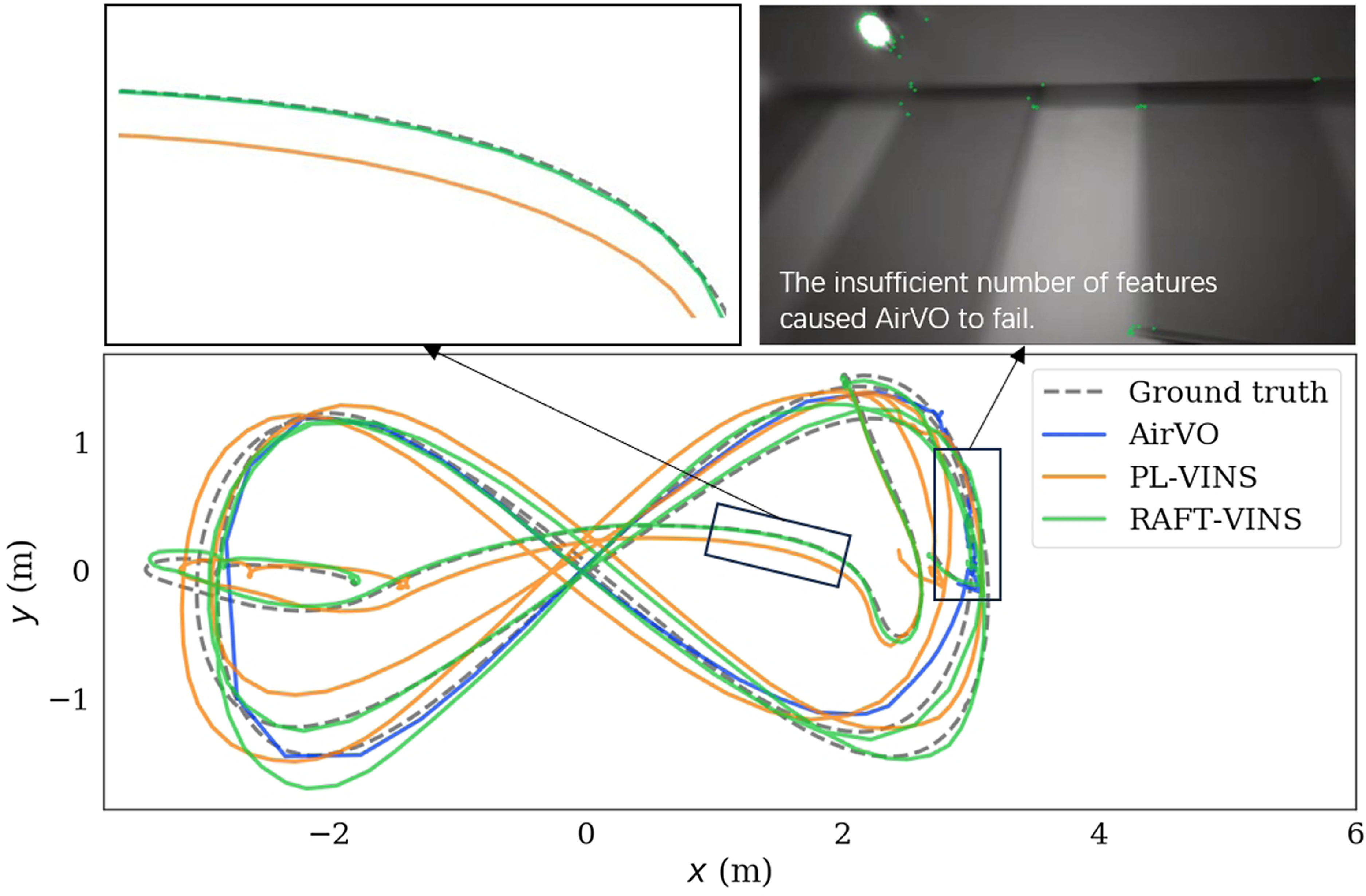
The real-world experiment trajectory compare.

The quantitative localization accuracy comparison is shown in Table V. On the circle sequence, our method’s performance is very close to that of PL-VINS and better than AirVO and VINS-Mono. On the eighth sequence, due to unstable feature tracking, VINS-Mono produces significant drift, and AirVO also loses features during the second lap of the eighth, causing the system to fail. Our method utilizes deep learning for optical flow tracking, which does not require continuous extraction of a large number of features, resulting in more stable performance. The real-world experiment trajectory comparison is shown in Figure 10.
4.4.4 Ablation Study
To demonstrate the effectiveness of the moving consistency check, we remove this component and conduct evaluations in real-world experiments. The results are shown in Table VI, indicating that the moving consistency check enhances accuracy effectively.
5. Conclusion
In this paper, we have proposed RAFT-VINS, an efficient and illumination-insensitive visual-inertial odometry designed to improve pose estimation accuracy in dynamic illumination environments. To overcome the challenges of feature association, we have designed a lightweight deep optical flow network and a moving consistency check strategy. Extensive experiments have been conducted to show the robustness, accuracy, and efficiency of RAFT-VINS, demonstrating its potential for pose estimation in dynamic illumination environments. In the future work, we will integrate additional learning-based techniques, such as monocular depth estimation, to further enhance its performance.
Ablation study. RAFT-VINS w/o mcc means RAFT-VINS without moving consistency check component. Translational error (root mean square error) comparison in real world.

Author contributions
In this article, Jie Zhang, Cong Zhang, Qingchen Liu, and Jiahu Qin conceived and designed the study. Jie Zhang and Cong Zhang conducted the experiments, data collection, and statistical analysis. Jie Zhang, Cong Zhang, and Qichao Ma wrote the article.
Financial support
This work was supported in part by the National Natural Science Foundation of China under Grant 62425309, Grant 62403444, and Grant 62373341, and in part by the China Postdoctoral Fellowship Program of CPSF under Grant GZC20232548.
Competing interest
The authors declare no conflicts of interest exist.
Ethical approval
Not applicable.
Supplementary material
The supplementary material for this article can be found at http://doi.org/10.1017/S0263574725000608.