2.1. Tests for a Single Unknown Break Point

Suppose that the model to be tested is indexed by a vector of parameters θ_t, where t is an index of time. The subscript indicates that the value of the parameter vector may change from period to period. The null hypothesis is that the parameters are constant throughout the sample, that is,

The alternative is that the parameter vector changes at a proportion π of the sample, that is, at time Tπ:

To perform this test, Andrews (1993) discusses GMM analogues of the three classical tests: Wald, likelihood ratio, and Lagrange multiplier. The exact form of the statistics may be found in that paper. Like their classical counterparts, these statistics are distributed asymptotically as chi squared when the break point parameter π is known. If π is unknown, but is suspected to lie in a proper subset of the unit interval, the break point may be estimated by locating the value of π that corresponds to the strongest indication of a break, that is, to the largest value of one of the three statistics. Andrews and Ploberger (1984) also consider statistics based on the average or exponential average value of the break statistic over a subset of the unit interval. In this paper, we focus on the tests based on the supremum of the statistic, which are widely used and have a direct intuitive interpretation.

Thus, let Π = [π₁,π₂] be a closed interval contained in (0,1) and let S be the set of observations from t = [π₁T] to t = [π₂T] , where [·] denotes rounding to the nearest integer, that is, S = {t|[π₁T] ≤ t ≤ [π₂T]}. Consider the supremum of the Wald (W), likelihood ratio (LR), or Lagrange multiplier (LM) statistic from among the values computed at every point in S and let ζ denote one of sup_S W, sup_S LR, or sup_S LM. Andrews (1993) shows that, under certain regularity conditions, the distribution of ζ is a function of multivariate Brownian motion, which may be constructed as follows.

Let B_p(·) be a p-dimensional vector of independent Brownian motions. Then ∥B_p(π)∥ = (B_p(π)′B_p(π))^1/2 is the Bessel process of order p and BB_p(π) = B_p(π) − πB_p(1), known as a Brownian bridge. If B_p(·) is defined on [0,1] and restricted to Π, then

is the square of the standardized tied-down Bessel process of order p.

When one of the GMM break tests is performed with a known value of π, the asymptotic distribution of the test statistic corresponds to Q_p(π), which in that case has a χ_p² distribution, as demonstrated by Andrews and Fair (1988). However, when π is unknown and is estimated by locating the supremum of one of the test statistics, Andrews (1993) shows that the relevant distribution is

where λ = π₂(1 − π₁)/π₁(1 − π₂). Note that the probability depends on π₁ and π₂, not individually, but only through λ. Note also that when π₁ = 1 − π₂ = π₀, then λ = ((1 − π₀)/π₀)². The interpretation of equation (4) is that the distribution of the supremum of the tied-down Bessel process is equivalent to the distribution of the supremum of the standard Bessel process exceeding a square-root boundary, which has been studied by DeLong (1981).

In addition to Andrews (1993), other papers have used Bessel process distributions to test for single unknown breaks in models. Among these are Siegmund (1986) for a single parameter, James, James, and Siegmund (1987) for multiple parameters, and Akman and Raftery (1986) for a single Poisson parameter.

Ghysels et al. (1997) introduce a test for multiple parameters, which is based on estimating the model by GMM over a portion of the sample and predicting the value of the GMM orthogonality conditions over the remaining portion. When the model is just-identified, their statistic measures the distance of the orthogonality conditions from zero, which would hold if the model fit perfectly over the remaining portion of the sample. In this case, the asymptotic distribution of the statistic is the same as in Andrews (1993).

2.2. Tests for Multiple Breakpoints

Some tests for multiple break points also use the Bessel process distribution from equation (4). For instance, Bai (1999) constructs a LR test for m + 1 breaks under the null of m breaks. Let 0 < φ₁ < ··· < φ_m < 1 be the proportions of the sample representing the m break points estimated under the null, with φ_i − φ_i−1 > π₀ for some small value π₀. Define also η_i = π₀ /(φ_i − φ_i−1), i = 1,…,m + 1, where we take φ₀ = 0 and φ_m+1 = 1.

The LR test is obtained by estimating m + 1 break points and comparing the likelihood to the m break likelihood. In this case, the distribution of the LR is asymptotically

Thus, p values for LR may be computed by repeated application of the formula for p values in the single-break case.

Bai and Perron (1998) also use the Bessel process distribution in tests for multiple break points. They develop two types of tests, one for no breaks vs. a fixed number k of breaks and the other a sequential test for m vs. m + 1 breaks. In the former, the asymptotic distribution is the Bessel process when k = 1, whereas in the sequential test, the asymptotic distribution is given by repeated application of the Bessel process, as in Bai (1999).

2.3. Other Statistical Applications

Bessel process distributions are also useful in statistical applications other than structural break tests. For instance, Anderson and Darling (1952) construct a variant of the Kolmogorov–Smirnov test for goodness of fit, whose distribution is given by the Bessel process. Siegmund (1985) is a comprehensive survey of sequential analysis tests, several of which are asymptotically distributed as the Bessel process. For instance, a repeated significance test for nonzero drift in Brownian motion W(t) is based on the first time that

within a time interval m₀ ≤ t ≤ m. Its distribution is essentially the same as (4). Siegmund (1986) contains a more detailed summary of these and other applications.

3.1. DeLong's Exact Formula

Equation (4) in the previous section presents two equivalent formulations for the asymptotic distribution of the supremum-based break tests, one in terms of the standardized tied-down Bessel process and one in terms of the Bessel process itself. In an important and influential paper, DeLong (1981) gives an exact expression for the Bessel process formulation, which involves the crossing of a square-root boundary. Virtually all the numerical applications of the Bessel process to break testing because 1981 correspond to approximations of DeLong's formula.

The reason for the use of approximations is the generally perceived intractability of the expression of DeLong (1981). In this section, we examine the expression and provide some results that simplify its calculation. With these results, we argue that the calculation is in fact fairly quick and simple and that there is little reason to resort to approximations.

To state DeLong's expression, let M(a,b,z) be the confluent hypergeometric function

where (a)_k ≡ a(a + 1)…(a + k − 1) is the Pochhammer symbol, with (a)₀ ≡ 1. The infinite series converges as long as b is not a negative integer. Let M₁(a,b,z) be the partial derivative of this function with respect to its first argument. DeLong (1981) shows that

where β_j is the jth root of M(β + p/2,p/2,−c/2) as a function of β > 0,

and Γ(·) is the gamma function.

Computationally, the only real challenge in this formula is the identification of the roots β_j. Once these values are known, the infinite sums in (6) and (7) converge quickly, and their computation to any desired degree of accuracy is straightforward. Let us therefore focus on the calculation of the roots β_j. The main problem is that there is an infinity of β_j, and there is no known closed-form expression for these values. However, given a relatively close first approximation

, Newton's method may be used to compute β_j accurately. Thus, how can

be obtained?

DeLong (1981) provides an asymptotic approximation (as j approaches infinity) that is very accurate for large values of j, and fairly accurate even for small j, unless the number of parameters p is large. Thus,

Newton's method could be applied using this value as an initial guess

. If β_j⁽ⁿ⁾ is the nth guess, the n + 1 approximation is given by

The derivative M₁ may be computed analytically or numerically, and β_j⁽ⁿ⁾ generally converges to β_j quickly.

The problem with this method is that

is not always sufficiently accurate, particularly if the value of p is large. In such cases, Newton's method may converge to the wrong β_j. A more reliable method, though computationally somewhat more costly, is to perform a grid search to identify the approximate location of each β_j and then to apply Newton's method using each approximate location as an initial approximation. Because of its reliability, an optimally constructed grid search is the preferable method.

Thus, consider a grid for β based on an increment of size δ > 0 and look successively at M(nδ + p/2,p/2,−c/2), n = 0,1,… until a change of sign is detected. If the sign changes for β between nδ and (n + 1)δ, Newton's method may be used locally to compute the zero.¹

PROPOSITION 1. Let m_n = M(n + b,b,z) for n = 0,1,…. Then m₀ = exp(z), m₁ = ((b + z)/b)m₀, and m_n+1 = (2 + (z − b)/(n + b))m_n + (b/(n + b) − 1)m_n−1 for n ≥ 1.

PROPOSITION 2. Let β_j and β_j+1 be two consecutive roots of M(β + p/2, p/2,−c/2) as a function of β > 0. Then |β_j+1 − β_j| = β_j+1 − β_j > 1.

PROPOSITION 3.

, so that α_j λ^−β_j > 0 for all j.

Proposition 2 implies that we can take δ = 1 with no danger of missing any of the roots β_j. Any interval one unit long contains at most one root, and this root is more than one unit away from the nearest roots. Moreover, to speed up the grid search, we may use the recursive formula in Proposition 1 and obviate the need to evaluate M at every point n = 0,1,…. Once a change is detected, specifically when m_n+1 m_n ≤ 0, we can find a root in the interval (m_n,m_n+1] using Newton's method. The initial guess is determined by linear interpolation in this interval.

This process may be used to continue identifying roots until the number of terms in the infinite sum in (7) is sufficient to obtain the desired level of accuracy. Proposition 3 implies that all the terms in (7) are positive and one may stop when the last term computed is smaller than some positive tolerance level.

3.2. Numerical Results

To check the accuracy of the computational method described previously, the method was used to replicate the relevant tables in DeLong (1981). DeLong's Table I (first four panels) contains probabilities that correspond to the application of (7) to 1,500 combinations of the parameters p, λ, and c. The method was applied with tolerance levels that provide accuracy to at least the four decimal places given by DeLong. The results matched DeLong's exactly in more than 98% of cases.

In cases where the results differ, DeLong's figure was always slightly lower, suggesting perhaps the inclusion of fewer terms from expression (7) (because all are positive by Proposition 3). Most differences were very minor, however, only 0.0001. A few larger differences were found only in cases in which p = 1 and c = 1. These differences were all less than 0.0042 and in most instances were much smaller. As a robustness check in light of these puzzling discrepancies, the method of Section 3.1 was applied with p = 1 and c = 1 ± ε, for small values of ε. The same results as with c = 1 were obtained.

DeLong's Table II presents critical values c, to two decimal places, corresponding to various combinations (375 altogether) of the parameters p and λ. This table was replicated by inverting the numerical probability function of Section 3.1, using another application of Newton's method. The results of DeLong's Table II were matched exactly.

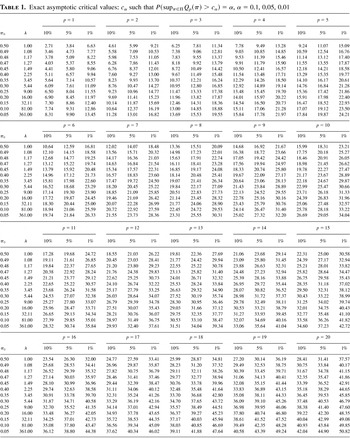
Finally, the method was used with the same tolerance level to recalculate Table 1 of critical values in Andrews (1993), which is widely cited as a reference in both the theoretical and applied literatures. Exact results are presented here in Table 1. Note that, following Andrews (1993), these results are tabulated according to π₀, the proportion of data points dropped at either end of the sample, rather than λ, as given in equation (4). Andrews calculates his figures by stochastic simulation of the Bessel process over the unit interval. These simulation results are subject to discretization bias and to sampling error. Discretization bias results because continuous Brownian motion is approximated using a large but finite number of normal distributions over small disjoint intervals. This bias is notoriously difficult to eliminate, even when using very small intervals.

Exact asymptotic critical values: cα such that P(supπ∈Π Qp(π) > cα) = α, α = 0.1, 0.05, 0.01

Andrews (1993) splits the unit interval into 3,600 segments, and yet his critical values tend to be a bit low, most likely as a result of discretization. In most cases, however, the approximations are reasonably close. Exceptions are the values for p = 8, which are particularly low for no obvious reason. Andrews (2003) provides a revised table based on a larger number of simulation iterations. The entries for p = 8 are no longer outliers, and the sampling error is reduced. However, some discretization bias remains.

Discretization does not necessarily lead to less accurate results, because the timing of observations in a finite sample maps to a discrete set of points in the unit interval, rather than the infinity of points corresponding to the asymptotic theory. However, use of the exact asymptotic distribution seems preferable in most applications. One important reason is that simple discretization assumes that increments are independent and normally distributed, a result that derives from the application of central limit theorems (as in Andrews, 1993, Theorem 1) in the asymptotic case. Assuming independence and normality directly in finite samples is possible but is much more restrictive than the typical assumptions of the asymptotic GMM approach.

4.1. Approximate Probability for Large c

Because DeLong's formula has been considered intractable, various researchers have proposed using an asymptotic approximation to the formula, which is accurate when c is large. In fact, DeLong (1981) himself derives such an approximation, though special cases had been known earlier. The approximation is based on an expansion of the probability from equation (4) in terms of powers of c. Specifically,

The asymptotic approximation is obtained by ignoring the term O(c⁻²) in (10), resulting in a closed-form expression as a function of the arguments p, λ, and c. Dirkse (1975) studies essentially the same distribution but with the Bessel process constructed from univariate Brownian motion (p = 1). He does not derive an expression for the exact probability but proceeds directly to the calculation of the asymptotic approximation, which matches (10) exactly (with p = 1).²

4.2. Accuracy of Asymptotic Approximation

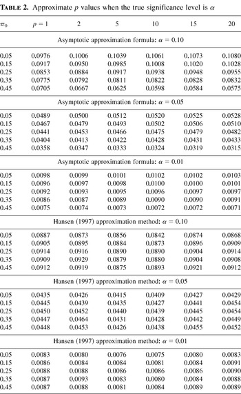
To gauge the accuracy of the asymptotic approximation, we perform the following experiment. First, using the exact distribution for a given set of parameter values, we obtain the critical value corresponding to a significance level α, where α is 10, 5, or 1%. Then, we apply the approximation formula to the critical value. The more accurate the approximation, the closer the resulting approximate p value will be to α. The first part of Table 2 provides results for selected values of p ranging from 1 to 20 and for selected values of π₀ ranging from 0.05 to 0.45. These ranges are likely to be representative of values encountered in practice.

Approximate p values when the true significance level is α

As the table indicates, results for π₀ = 0.05 and 0.15 are quite accurate for all three significance levels, particularly for α = 0.01. This pattern is explained by the assumptions underlying the asymptotic approximation, which correspond to low values of both α and π₀. To see this, note that in DeLong's derivation, he makes the assumption that λ is large and, correspondingly, that π₀ is small. Moreover, the result is obtained by allowing the critical value c to be arbitrarily large, which corresponds to an arbitrarily low significance level α. When π₀ = 0.25, the results deteriorate somewhat, and the errors are more pronounced for larger π₀, particularly when both π₀ and p are large. For instance when π₀ = 0.45, p = 20, and the true significance level is 10%, the formula produces an approximate significance level of 5.75%.