Hyperbolic foliated entropy of suspensions

FRANÇOIS BACHER

doi:10.1017/etds.2026.10341

Hyperbolic foliated entropy of suspensions

Part of: Locally compact groups and their algebras Complex dynamical systems Topological dynamics Ergodic theory

Published online by Cambridge University Press: 24 September 2026

FRANÇOIS BACHER

Show author details

FRANÇOIS BACHER*: Affiliation:
Institut de mathématiques de Bourgogne, Université Bourgogne Europe , France
*: e-mail: francois.bacher@u-bordeaux.fr

Article contents

Abstract
Introduction
Laminations, suspensions and hyperbolic entropy
Some hyperbolic geometry
Comparing entropies
Measure-theoretic entropy
References

Rights & Permissions

Abstract

We study the hyperbolic entropies of foliations obtained by suspensions of a representation in the sense of Dinh, Nguyên and Sibony (topological and measure-theoretic). We establish a link between this type of entropy and an adapted version of an entropy defined by Ghys, Langevin and Walczak for pseudo-groups of homeomorphisms. Such a link has various consequences. Among them, it implies that the hyperbolic entropy of foliations is not invariant by diffeomorphisms, and that a minimal entropy suspension admits an invariant measure. Finally, this allows us to study thoroughly the simple case in which the image of the representation is isomorphic to $\mathbb {Z}$. In that case, we give the first exact estimate of the hyperbolic entropy, and prove a Brin–Katok-type theorem and a variational principle, relying strongly on the standard ones for the entropy of maps.

Keywords

holomorphic foliations topological hyperbolic entropy metric hyperbolic entropy suspensions

MSC classification

Primary: 37F75: Holomorphic foliations and vector fields 37A15: General groups of measure-preserving transformations

Secondary: 37B40: Topological entropy 22D40: Ergodic theory on groups

Information

Type: Original Article
Information: Ergodic Theory and Dynamical Systems , First View , pp. 1 - 25

DOI: https://doi.org/10.1017/etds.2026.10341 [Opens in a new window]
Copyright: © The Author(s), 2026. Published by Cambridge University Press

1 Introduction

The dynamical theory of laminations by Riemann surfaces has received much attention in the last twenty years. In particular, much research has been focused on the case where all the leaves are hyperbolic Riemann surfaces. In the case of foliations on projective spaces, this is the most common setup. Indeed, every polynomial vector field on $\mathbb {C}^n$ induces a singular holomorphic foliation on $\mathbb {P}^n$ . For generic foliations of degree at least $2$ , all the leaves are hyperbolic. This result is due to Jouanolou [Reference Jouanolou23], Lins Neto and Soares [Reference Lins Neto and Soares27], Lins Neto [Reference Lins Neto26] and Glutsyuk [Reference Glutsyuk22]. In that case, considering Brownian motions, one can define Lyapunov exponents of a measure. When $n=2$ , Nguyên uses the integrability of the holonomy cocycle [Reference Nguyên29] to compute exactly the Lyapunov exponent [Reference Nguyên31] of the unique ergodic measure of a generic foliation obtained by Fornæss and Sibony [Reference Fornæss and Sibony16]. It is worth noting that the unique ergodicity is extended later by Dinh, Nguyên and Sibony [Reference Dinh, Nguyên and Sibony12] to a generic foliation on every compact Kähler surface. We refer the reader to the survey articles [Reference Dinh and Sibony13, Reference Fornæss and Sibony15, Reference Nguyên28, Reference Nguyên30] for a more detailed exposition of this theory.

Here, we are mostly interested in an ergodic theory for laminations by hyperbolic Riemann surfaces. Solving heat equations with respect to harmonic currents, Dinh, Nguyên and Sibony [Reference Dinh, Nguyên and Sibony9] obtain an effective geometric analog of the Birkhoff theorem. In this theorem, the quantity that plays the role of time is the Poincaré distance in the uniformization of the leaves by the hyperbolic disk, and the usual invariant measures are replaced by harmonic measures. Indeed, many foliations do not admit any invariant measure. Since Garnett [Reference Garnett19] (respectively, Berndtsson and Sibony [Reference Berndtsson and Sibony4]) shows that any compact lamination (respectively, any compact holomorphic foliation with isolated singularities) does admit harmonic ones, we need to consider them. The hyperbolic interpretation of time then leads to notions of entropy, both measure-theoretic and topological, that the three authors define in a series of two articles [Reference Dinh, Nguyên and Sibony10, Reference Dinh, Nguyên and Sibony11].

Let us introduce some notation and give a rough definition of the entropy (see §2.2 for a more precise treatment). Let $\mathscr {F}=(X,\mathscr {L})$ be a lamination by hyperbolic Riemann surfaces, with $(X,d_X)$ a compact metric space. Then all the leaves are uniformized by the Poincaré disk and one can choose parametrizations $\phi _x\colon \mathbb {D}\to L_{x}$ such that $\phi _x(0)=x$ , for $x\in X$ , where $L_{x}$ is the leaf passing through $x$ . For $R>0$ , define a Bowen distance

(1.1) $$ \begin{align}d_R(x,y)=\inf_{\theta\in\mathbb{R}}\sup_{\xi\in\overline{\mathbb{D}}_{R}}\,d_X(\phi_x(\xi),\phi_y(e^{i\theta}\xi)),\end{align} $$

where $\mathbb {D}_{R}\subset \mathbb {D}$ is the disk of hyperbolic radius $R$ centered at $0$ . Note that the infimum over all possible parametrizations ensures that $d_R$ is independent of the choice of the $\phi _x$ , for $x\in X$ . Given Bowen balls, Dinh, Nguyên and Sibony can define a topological entropy $h(\mathscr {F})$ in the usual Bowen way. It measures the exponential rate with $R$ , at which leaves go apart with respect to $d_R$ . Also, given a harmonic measure $\mu $ , one can consider quantities introduced by Katok [Reference Katok24] and Brin and Katok [Reference Brin and Katok6] as definitions for a measure-theoretic entropy $h(\mu )$ , and for local upper and lower entropies $h^{\pm }(\mu ,x)$ , respectively (see §5).

So far, little is known about these quantities. They are finite (with no upper bound) in some cases [Reference Bacher3, Reference Dinh, Nguyên and Sibony10, Reference Dinh, Nguyên and Sibony11]. If $\mu $ is ergodic and with additional assumptions [Reference Bacher2, Reference Dinh, Nguyên and Sibony10], the $h^{\pm }(\mu ,x)$ are known to be constant almost everywhere and we have

$$ \begin{align*}2\leq h^-(\mu)\leq h(\mu)\leq h^+(\mu)\leq h(\mathscr{F}).\end{align*} $$

In particular, there is no clear interpretation of the fact that the entropy is minimal, that is, equal to 2, nor is there any known non-trivial example in which it is computable. We expect, as in the Brin–Katok theorem, that one could show $h^-(\mu )=h^+(\mu )$ . We also hope to find a variational principle $h(\mathscr {F})=\sup _{\mu }h(\mu )$ , but no example can argue in favor of such a belief. As a matter of fact, there is not even a written example on which it is known to be greater than $2$ .

The aim of this note is to give first examples of explicit bounds and values for these entropies with suspensions. Consider a compact smooth Riemann surface $\Sigma $ of genus ${g\geq 2}$ and a representation $\rho \colon \Gamma =\pi _1(\Sigma )\to \operatorname {\mathrm {Homeo}}(T)$ , where $(T,d)$ is a compact metric space. Then $\Gamma $ acts diagonally on $\mathbb {D}\times T$ , and $X=(\mathbb {D}\times T)/\Gamma $ is foliated by the image of horizontal disks $\mathbb {D}\times \{t\}$ , $t\in T$ (see §2.3). From the point of view of the entropies, such a lamination has the advantage of having completely explicit parametrizations $\phi _x$ , for $x\in X$ . Hence, we can compare the entropy $h(\mathscr {F})$ with that given by the holonomy $\rho $ . More precisely, given a symmetric set of generators $\mathcal {G}$ of $\Gamma $ , Ghys, Langevin and Walczak [Reference Ghys, Langevin and Walczak21] define a Bowen distance for $N\in \mathbb {N}$ , and for $t,s\in T$ ,

$$ \begin{align*}d_N(t,s)&=\sup\{d(\rho(g_1\ldots g_n)(t),\rho(g_1\ldots g_n)(s));~n\leq N,~g_1,\ldots,g_n\in\mathcal{G}\},\end{align*} $$

Here, the quantity that plays the role of time is the word distance in $\Gamma $ with generators $\mathcal {G}$ . As usual, a Bowen distance induces an entropy. Here, we use the same kind of distance with a weight $\omega \colon \mathcal {G}\to \mathbb {R}_+^*$ 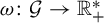, to define an entropy $h(\rho ,\mathcal {G},\omega )$ , closely related to that of Ghys, Langevin and Walczak. Our main result is the following theorem (see Theorem 4.10 for a more precise statement).

Theorem 1.1. Consider a suspension as above. There exists $K=K(\Gamma )>1$ such that

$$ \begin{align*}2+h(\rho,\mathcal{G},\omega)\leq h(\mathscr{F})\leq 2+Kh(\rho,\mathcal{G},\omega).\end{align*} $$

In particular, this has the following consequences. For the second one, we use a result of Ghys, Langevin and Walczak [Reference Ghys, Langevin and Walczak21].

Corollary 1.2 (Proposition 4.11).

Entropy is not a smooth invariant of laminations.

Corollary 1.3 (Proposition 5.4).

Let $\mathscr {F}$ be a suspension with entropy $2$ . Then $\mathscr {F}$ admits an invariant measure.

Next, we consider the measure-theoretic entropies. For suspensions, Alvarez [Reference Alvarez1] shows that for a well-chosen probability measure $m$ on $\Gamma $ , there is a one-to-one correspondence between $m$ -stationary measures on $T$ and harmonic measures on $\mathscr {F}$ , for which invariant measures correspond to invariant measures. So, we obtain the same kind of comparison of the measure-theoretic entropies $h^-(\mu ),h(\mu ),h^+(\mu )$ , with entropies of the action of $\Gamma $ on $T$ . In particular, when the image of $\rho $ in $\operatorname {\mathrm {Homeo}}(T)$ is generated by a single map $f$ , we obtain the following link with the usual topological entropy $h_{\mathrm {top}}(f)$ and the usual measure-theoretic entropy $h_{\nu }(f)$ of $f$ .

Theorem 1.4 (Theorem 5.8).

In the above setup, let $\mu $ be an ergodic harmonic measure on $\mathscr {F}$ and $\nu $ be the corresponding $m$ -stationary measure on $T$ given by Alvarez [Reference Alvarez1]. Then $\mu $ and $\nu $ are in fact invariant and there exists a $K_0>0$ such that:

• $h(\mathscr {F})=2+2K_0h_{\mathrm {top}}(f)$ ;
• $h^-(\mu )=h(\mu )=h^+(\mu )=2+2K_0h_{\nu }(f)$ .

In particular, we have the variational principle $h(\mathscr {F})=\sup _{\mu }h(\mu )$ .

Let us briefly describe the proofs of these results. The main problem is to compare on the one hand word distance (with weight) in $\Gamma $ , with generators $\mathcal {G}$ ; and on the other hand the Poincaré distance to $0$ in the disk. More precisely, the weight $\omega \colon \mathcal {G}\to \mathbb {R}_+^*$ 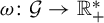is defined so that, for $\alpha =g_1\ldots g_n\in \Gamma $ , $d_{P}(0,\alpha (0))$ is comparable to $\sum _{i=1}^n\omega (g_i)$ 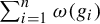. This result is obtained in Proposition 3.5. The second problem is to show that we can restrict our attention to a transversal and to the holonomy $\rho $ . This is done in §4.2, in which we show that we can decompose the entropy into a leafwise one equal to $2$ , and a transversal one given by the holonomy. Here, the arguments are very similar to [Reference Bacher2, Reference Dinh, Nguyên and Sibony10, Reference Dinh, Nguyên and Sibony11]. A crucial property that we show, is that one can get rid of the reparametrization issue in the definition (1.1) of $d_R$ , by choosing canonical parametrizations, and that one still computes the same entropy. Finally, similar gymnastics of a different Bowen distance for the same entropy give us that the transversal entropy is comparable to $h(\rho ,\mathcal {G},\omega )$ , as in Theorem 1.1.

Our more precise results for the measure-theoretic entropy come from a subadditive argument. If $f$ is a generator of $\rho (\Gamma )$ , we show that at the limit, the maximal power $f^{n(R)}$ represented in $\mathbb {D}_{R}$ is essentially $n(R)=K_0R$ , for some constant $K_0$ . Therefore, all that remains to do is to adapt the proof of the Brin–Katok theorem to an invertible case, that is, to powers of $f$ between $-n(R)$ and $n(R)$ , instead of from $0$ to $n$ .

The paper is organized as follows. In §2, we present the notions of lamination, topological entropy, and suspension. In §3, we recall well-known facts about Fuchsian groups and prove our comparison of word distance and hyperbolic distance. In §4, we start by constructing the weighted entropy $h(\rho ,\mathcal {G},\omega )$ , then we show that we can restrict our attention to the transversal, and we prove the main theorem. Finally, in §5, we recall the basics about invariant, stationary and harmonic measures and Alvarez’s theorem, before proving Theorem 1.4.

1.1 Notation

Throughout this paper, we denote by $\mathbb {D}$ the unit disk of $\mathbb {C}$ . For $R\in \mathbb {R}_+^*$ , we also denote by $\mathbb {D}_{R}=\{\xi \in \mathbb {D};~d_{P}(0,\xi )<R\}$ the open disk of hyperbolic radius $R$ in $\mathbb {D}$ , where $d_{P}(0,\xi )=\ln [({1+\vert \xi \vert })/({1-\vert \xi \vert })]$ is the Poincaré distance between $0$ and $\xi $ .

We will also consider a distance $d=d_X$ on an ambient compact metric space $X$ , coming from a Riemannian metric on a manifold $M$ . For $\phi ,\psi \colon K\to X$ or $\tau ,\sigma \colon K\to \mathbb {D}$ (typically, $K=\overline {\mathbb {D}}_{R}$ , and the maps are in fact defined on whole $\mathbb {D}$ ), we write

$$ \begin{align*}d_K(\phi,\psi)=\sup_{\xi\in K}\,d(\phi(\xi),\psi(\xi)),\quad d_{P,K}(\tau,\sigma)=\sup_{\xi\in K}\,d_{P}(\tau(\xi),\sigma(\xi)).\end{align*} $$

For integers $p\leq q\in \mathbb {Z}$ , we denote by ${[\![} p,q{]\!]} =\{p,p+1,\ldots ,q-1,q\}$ the integer interval between $p$ and $q$ . If $x$ is a real number, we denote by $\lfloor x\rfloor $ and $\lceil x\rceil $ the floor and ceiling parts of $x$ . That is, $\lfloor x\rfloor $ (respectively, $\lceil x\rceil $ ) is the greatest (respectively, smallest) integer $p\in \mathbb {Z}$ such that $p\leq x$ (respectively, $p\geq x$ ).

Finally, we use $C$ , $C'$ , $C"$ , etc. to denote positive constants which may change from line to line.

2 Laminations, suspensions and hyperbolic entropy

2.1 Basics about laminations

In this section, we recall some concepts in the context needed for this paper. In particular, we will not define laminations in the broadest sense. The reader may consult [Reference Nguyên30] for a more general definition.

Definition 2.1. Let $(X,d_X)$ be a compact metric space. A lamination by Riemann surfaces (henceforth, ‘lamination’) $\mathscr {F}=(X,\mathscr {L})$ on $X$ is the data of an atlas $\mathscr {L}$ of $X$ , given by homeomorphisms

$$ \begin{align*}\Phi_i\colon U_i\to\mathbb{D}\times\mathbb{T}_i,\end{align*} $$

where $(U_i)_{i\in I}$ is an open covering of $X$ , $\mathbb {T}_i$ are topological spaces (the transversals), and the transition maps $\Phi _{ij}=\Phi _i\circ \Phi _j^{-1}$ are of the form

(2.1) $$ \begin{align}\mathbb{D}\times\mathbb{T}_j\to\mathbb{D}\times\mathbb{T}_i,\quad (z,t)\mapsto(\psi_{ij}(z,t),\unicode{x3bb}_{ij}(t)),\end{align} $$

with $\psi _{ij}$ holomorphic in $z$ and continuous in $t$ and $\unicode{x3bb} _{ij}$ continuous.

If the maps $\psi _{ij}$ and $\unicode{x3bb} _{ij}$ have more regularity, for example if they are $\mathscr {C}^{r}$ , Lipschitz, etc., we will say that the lamination $\mathscr {F}$ is $\mathscr {C}^{r}$ , Lipschitz, etc.

A coordinate chart $U\simeq \mathbb {D}\times \mathbb {T}$ as above is called a flow box. The level sets ${\Phi _i^{-1}(\mathbb {D}\times \{t\})}$ 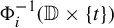, for $t\in \mathbb {T}_i$ are called plaques. The form (2.1) of the transition maps ensures that the plaques are compatible, in the sense that two different plaques either have empty intersection, or have an open subset of $\mathbb {D}$ in common. A non-empty connected subset of $X$ which contains each plaque it intersects, and which is minimal for this property, is called a leaf of $\mathscr {F}$ . The fact that $\psi _{ij}$ is holomorphic in $z$ in (2.1) implies that a leaf $L$ of $\mathscr {F}$ inherits a Riemann surface structure.

Here, we will only consider laminations which are embedded in a real manifold $M$ . That way, using a partition of unity, one can build a smooth Riemannian metric $g_{M}$ , which restricts to a Hermitian metric on the plaques. We also suppose that the distance $d_X$ on $X$ is that coming from the distance induced by $g_{M}$ on $M$ . This is actually the only reason why we need to consider embedded laminations.

We are mainly interested in laminations, the leaves of which are all hyperbolic Riemann surfaces. If $\mathscr {F}=(X,\mathscr {L})$ is such a lamination, denote by $g_{P}{}$ the leafwise Poincaré metric. Two Hermitian metrics on a Riemann surface being pointwise proportional, there exists a map

$$ \begin{align*}\eta\colon X\to\mathbb{R}_+^*\quad\text{such that}\quad \eta^2g_{P}{}=g_{M}.\end{align*} $$

On the right-hand side of the above equation, we still denote by $g_{M}$ its restriction to the tangent space to the leaves of $\mathscr {F}$ . When $X$ is compact, it is easy to see [Reference Dinh, Nguyên and Sibony10, pp. 572] (and in the context of suspensions as in §2.3, the arguments can be made even simpler) that there exists a constant $c_0>1$ such that

(2.2) $$ \begin{align}c_0^{-1}\leq\eta(x)\leq c_0,\quad x\in X.\end{align} $$

2.2 Hyperbolic entropy

Consider a lamination $\mathscr {F}=(X,\mathscr {L})$ , the leaves of which are hyperbolic, where $(X,d_X)$ is a compact metric space. For each $x\in X$ , denote by $L_{x}$ the leaf of $\mathscr {F}$ through $x$ and by $\phi _x\colon \mathbb {D}\to L_{x}$ a uniformization of $L_{x}$ such that $\phi _x(0)=x$ . Such a uniformization is unique up to precomposition by a rotation.

Definition 2.2. [Reference Dinh, Nguyên and Sibony10, §3]

For $R>0$ , write $\mathbb {D}_{R}=\{\xi \in \mathbb {D};~d_{P}(0,\xi )<R\}$ , where $d_{P}{}$ is the Poincaré distance on $\mathbb {D}$ . Define the Bowen distance

(2.3) $$ \begin{align}d_R(x,y)=\inf_{\theta\in\mathbb{R}}\sup_{\xi\in\overline{\mathbb{D}}_{R}}\,d_X(\phi_x(\xi),\phi_y(e^{i\theta}\xi)),\quad x,y\in X.\end{align} $$

Such a quantity measures the distance between the orbits of $x$ and $y$ until hyperbolic time $R$ , up to reparametrization by a rotation. Clearly, it is independent of the choice of uniformizations $\phi _x,\phi _y$ . The ball of center $x\in X$ and radius $\varepsilon \in \mathbb {R}_+^*$ for the distance $d_R$ will be denoted by $B_R(x,\varepsilon )$ and called the R-Bowen ball of center x and radius $\varepsilon $ .

For $R,\varepsilon>0$ and $Y\subset X$ , denote by $N(Y,R,\varepsilon )$ (respectively, $N'(Y,R,\varepsilon )$ ) the minimal $N\in \mathbb {N}$ such that there exist $x_1,\ldots ,x_N\in X$ (respectively, $x_1,\ldots ,x_N\in Y$ ) with

$$ \begin{align*}Y\subset\bigcup\limits_{i=1}^NB_R(x_i,\varepsilon).\end{align*} $$ upper Y subset of union Underscript i equals 1 Overscript upper N Endscripts upper B Subscript upper R Baseline left parenthesis x Subscript i Baseline comma epsilon right parenthesis period

The subset $\{x_1,\ldots ,x_N\}$ is called the $(R,\varepsilon )$ -covering of Y (respectively, $(R,\varepsilon )$ -dense in Y). Also, denote by $M(Y,R,\varepsilon )$ the maximal $M\in \mathbb {N}$ such that there exist ${x_1,\ldots ,x_M\in Y}$ with the $B_R(x_i,\varepsilon )$ , $i\in \{1,\ldots ,M\}$ , pairwise disjoint. The subset $\{x_1,\ldots ,x_M\}$ is called $(R,\varepsilon )$ -separated in Y.

Such numbers are in fact closely related to each other, as can be seen in the following lemma.

Lemma 2.3. (Dinh–Nguyên–Sibony [Reference Dinh, Nguyên and Sibony10, Proposition 3.1])

In the above setup, we have

$$ \begin{align*}N(Y,R,\varepsilon)\leq N'(Y,R,\varepsilon)\leq M(Y,R,\varepsilon)\leq N(Y,R,\varepsilon/2).\end{align*} $$

Definition 2.4. [Reference Dinh, Nguyên and Sibony10, §3]

For $Y\subset X$ , the hyperbolic entropy of Y is defined as the quantity

(2.4) $$ \begin{align}h(Y)=\sup_{\varepsilon>0}\limsup_{R\to+\infty}\frac{1}{R}\log N(Y,R,\varepsilon).\end{align} $$ h left parenthesis upper Y right parenthesis equals sup Underscript epsilon greater than 0 Endscripts limit sup Underscript upper R right arrow plus infinity Endscripts StartFraction 1 Over upper R EndFraction log upper N left parenthesis upper Y comma upper R comma epsilon right parenthesis period

For $Y=X$ , we denote it by $h(\mathscr {F})$ . By Lemma 2.3, the same equivalent definition could have been made with the numbers $N'(Y,R,\varepsilon )$ or $M(Y,R,\varepsilon )$ .

Remark 2.5. The above entropy will sometimes be referred as a topological entropy, as opposed to a measure-theoretic entropy (see §5). As we will see in Proposition 4.11, it is not necessarily invariant under homeomorphisms, so this may not be the best choice of terminology.

On the other hand, for compact laminations, it is easy to check that it is independent of the choice of the Riemannian metric $g_{M}$ . Also, it is invariant under applications which are transversally continuous and leafwise biholomorphic.

Remark 2.6. This setup can be made much more general by considering a metric space $X$ and a family of distances $(d_R)_{R\geq 0}$ on $X$ . In practice, we suppose that $d_0=d_X$ , that $d_R$ increases with $R$ , and most of the time the distances $d_R$ are continuous with respect to $d_X$ . Then there is a notion of $d_R$ -balls of radius $\varepsilon $ , of covering, dense and separated subsets. Lemma 2.3 still holds and one can define an entropy for this family of distances by formula (2.4). See [Reference Dinh, Nguyên and Sibony10, §3] for various dynamically meaningful setups. This is something we will constantly do, for families of distances that will induce the same entropy (or a comparable one) as that of $d_R$ . See, for example, §4.1 or Remark 4.8.

2.3 Suspensions

Consider a compact smooth Riemann surface $\Sigma $ of genus $g\geq 2$ and denote by $\Gamma =\pi _1(\Sigma )$ its fundamental group. More details about the structure of $\Gamma $ will be recalled in the next subsection. For now, consider a representation $\rho \colon \Gamma \to \operatorname {\mathrm {Homeo}}(T)$ , where $T$ is a compact metric space. Then $\Gamma $ acts diagonally on $\mathbb {D}\times T$ by

$$ \begin{align*}\Gamma\times(\mathbb{D}\times T)\to\mathbb{D}\times T,\quad\gamma\cdot(z,t)=(\gamma\cdot z,\rho(\gamma)(t)),\end{align*} $$

where $\gamma \cdot z$ is the action by deck transformations of $\gamma \in \pi _1(\Sigma )$ on a fixed uniformization $\mathbb {D}\to \Sigma $ . Since the action of $\Gamma $ on $\mathbb {D}$ is free, properly discontinuous and cocompact, it is also such on $\mathbb {D}\times T$ . Therefore, if we define

$$ \begin{align*}X=(\mathbb{D}\times T)/\Gamma,\end{align*} $$

then $X$ is compact. We will suppose that it is embedded in a real manifold $M$ (this is the case if, for example, $T$ is itself a real manifold), to inherit a well-chosen Riemannian structure. For $A\subset \mathbb {D}\times T$ , denote by $[A]$ its image under the quotient map $\mathbb {D}\times T\to X$ . Then $X$ is laminated by the hyperbolic Riemann surfaces $[\mathbb {D}\times \{t\}]$ , for $t\in T$ . All these leaves are coverings of $\Sigma $ . Note $\mathscr {F}=(X,\mathscr {L}){}$ in this lamination. It is called the suspension of the representation $\rho $ .

Above, we presented suspensions in the context that is necessary to define our entropy, that is, that of hyperbolic leaves. The reader can consult [Reference Camacho and Lins Neto7, Ch. V, §4] for a broader definition. In our setup, Ghys [Reference Ghys20, pp. 51–52] (see also [Reference Nguyên30, Example 2.31]) shows that when $T=\mathbb {P}^1$ and $\rho (\Gamma )\subset \operatorname {\mathrm {Aut}}(\mathbb {P}^1)$ , $X$ is an algebraic surface that can be embedded in $\mathbb {P}^N$ , for some $N\geq 3$ .

From the point of view of entropy, suspensions constructed as above have the important and simple property that the covering maps of the leaves are completely explicit. This will allow us to have good estimates of entropy, in terms of the representation $\rho $ .

More precisely, denote $\mathbb {T}_0=[\{0\}\times T]$ . This is a global transversal to the lamination $\mathscr {F}$ , which is isomorphic to $T$ and will be called the distinguished transversal. We will sometimes blur the distinction between a point $t\in T$ and the point $[0,t]\in \mathbb {T}_0$ . For $t\in T$ , denote by $\phi _t$ the uniformization of the leaf $L_{t}$ passing through $t$ given by

(2.5) $$ \begin{align}\phi_t\colon\mathbb{D}\to L_{t},\quad z\mapsto[z,t].\end{align} $$

It is of course such that $\phi _t(0)=t$ (with $t\simeq [0,t]$ ), as in the notation of §2.2.

3 Some hyperbolic geometry

For this section, our main references are the books by Katok [Reference Katok25] and by Farb and Margalit [Reference Farb and Margalit14]. We will only focus on the hyperbolic geometry needed for further estimates of entropy. Also, as far as Fuchsian groups are concerned, we will only consider those which are fundamental groups of smooth compact Riemann surfaces. The reader is invited to consult the aforementioned books for a more complete presentation.

3.1 Cocompact Fuchsian groups

In this subsection, we recall the definition of a Fuchsian group, with a focus on those which are fundamental groups of compact smooth hyperbolic Riemann surfaces.

Definition 3.1. A Fuchsian group is a subgroup $\Gamma $ of $\operatorname {\mathrm {Aut}}(\mathbb {D})$ that acts properly and discontinuously on $\mathbb {D}$ , that is, for every compact $K$ of $\mathbb {D}$ , $\{\alpha \in \Gamma ;~\alpha (K)\cap K\neq \emptyset \}$ is finite.

If $\Gamma $ is a Fuchsian group, the quotient $\Sigma =\mathbb {D}/\Gamma $ is a hyperbolic Riemann surface (with possibly orbifold singularities). We say that $\Gamma $ is cocompact if $\Sigma $ is compact.

Moreover, $\Sigma $ is smooth if and only if every element of $\Gamma $ besides the identity has no fixed point in $\mathbb {D}$ , in which case $\pi _1(\Sigma )=\Gamma $ (see [Reference Katok25, §3.6]). Conversely, let $\Sigma $ be a compact smooth hyperbolic Riemann surface and let $\phi \colon \mathbb {D}\to \Sigma $ be a uniformization of $\Sigma $ . Then one can write $\Sigma =\mathbb {D}/\Gamma $ , with $\Gamma =\pi _1(\Sigma )$ being a Fuchsian group acting by deck transformations on $\mathbb {D}$ , and every element of $\Gamma $ besides the identity having no fixed point.

The next three results gather together some very well-known facts we will use about Fuchsian groups.

Proposition 3.2. [Reference Katok25, Corollary 4.2.3]

With the notation above, $\Sigma $ is compact if and only if $\Gamma $ has a compact fundamental domain $D$ .

Proposition 3.3. [Reference Farb and Margalit14, 10.4.1]

Consider two smooth compact Riemann surfaces ${\Sigma _i=\mathbb {D}/\Gamma _i}$ of genus $g_i\geq 2$ , for $i\in \{1,2\}$ . Then $\Sigma _1$ and $\Sigma _2$ are homeomorphic if and only if they are diffeomorphic, if and only if $\Gamma _1$ and $\Gamma _2$ are group-isomorphic, if and only if $g=g_1=g_2$ . In that case, the $\Gamma _i$ have the representation

$$ \begin{align*}\Gamma_i=\langle\alpha_1,\ldots,\alpha_g,\beta_1,\ldots,\beta_g~\vert~\alpha_1\beta_1\alpha_1^{-1}\beta_1^{-1}\ldots\alpha_g\beta_g\alpha_g^{-1}\beta_g^{-1}=\operatorname{\mathrm{id}}\rangle.\end{align*} $$

We now prove a simple result that will be useful in §4.4 to provide examples of diffeomorphic suspensions having different entropies.

Proposition 3.4. Let $g\in \mathbb {N}$ with $g\geq 2$ and $\varepsilon>0$ . Then there exists a Fuchsian group $\Gamma _{\varepsilon }$ , with $\mathbb {D}/\Gamma _{\varepsilon }$ a compact smooth Riemann surface of genus $g$ , a set of generators $\mathcal {G}_{\varepsilon }$ of $\Gamma _{\varepsilon }$ with $\mathcal {G}_{\varepsilon }=\mathcal {G}_{\varepsilon }^{-1}$ , $\operatorname {\mathrm {id}}\notin \mathcal {G}_{\varepsilon }$ , and an element $\alpha _{\varepsilon }\in \mathcal {G}_{\varepsilon }$ such that $d_{P}(0,\alpha _{\varepsilon }(0))\leq \varepsilon $ .

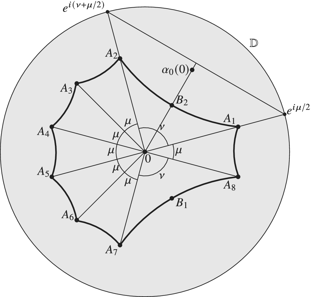
Proof. The proof goes as for Poincaré’s theorem [Reference Katok25, Theorem 3.4.2]. Consider a convex $4g$ -gon, bounded by geodesics, the vertices of which are $re^{i\theta _j}$ , $j\in {[\![} 1,4g{]\!]} $ , with $\theta _1=\mu /2$ , $\theta _2=\mu /2+\nu $ , $\theta _{j+1}=\theta _j+\mu $ , $j\in {[\![} 2,4g-2{]\!]} $ , $\theta _{4g}=\theta _{4g-1}+\nu =2\pi -\mu /2$ (see Figure 1). In other words, we choose one big angle $\nu $ and one small angle $\mu $ , with $2\nu +(4g-2)\mu =2\pi $ , put $4g$ points on a circle with two pairs of them at angle $\nu $ and the others at angle $\mu $ , so that the two big geodesics are separated by only one geodesic. Write $A_j=re^{i\theta _j}$ and denote by $D$ the closed $4g$ -gon bounded by the geodesics $A_jA_{j+1}$ , $j\in {[\![} 1,4g{]\!]} $ , with $A_{4g+1}=A_1$ . Now, as for Poincaré’s theorem, the sum of the internal angles of $D$ goes to $(4g-2)\pi $ when $r$ goes to $0$ , and to $0$ when $r$ goes to $1$ . So, there is an $r\in (0,1)$ such that this sum is $2\pi $ , and the usual identification of the sides of $D$ defines a Fuchsian group (see [Reference Farb and Margalit14, 10.4.2]).

Figure 1

The polygon $D$ , for some $r\in (0,1)$ and $g=2$ , in the proof of Proposition 3.4.

A geometric diagram of an eight-sided polygon with curved edges inscribed within a unit disk D, centered at origin O. See long description.

Figure 1 Long description

The diagram is centered at a point labeled 0. Radiating from this center are several line segments connecting to the vertices of a concave octagon. The vertices are labeled A sub 1 through A sub 8 in a counter-clockwise direction starting from the right.

* At the center, 6 angles between the radial lines are marked with the Greek letter mu. Two larger angles on the right side are marked with the Greek letter nu.

* The polygon has thick, inward-curving edges. Points B sub 1 and B sub 2 are marked at the middle of the edges between A sub 7 and A sub 8, and A sub 1 and A sub 2 respectively.

* The entire polygon is contained inside the unit disk D.

* Two points on the unit circle are labeled with complex exponentials: e super i mu forward slash 2 on the half line from O to A sub 1, and e super i open parenthesis nu plus mu forward slash 2 close parenthesis on the half line from O to A sub 2.

* A line segment connects these two boundary points, and a perpendicular bisector from the center 0 passes through B sub 2 to a point labeled alpha sub 0 open parenthesis 0 close parenthesis.

We wish to show that it satisfies our condition. Denote by $\alpha _0$ the generator sending the geodesic $(A_{4g-1}A_{4g})$ to the geodesic $(A_1A_2)$ . It is enough to prove that for well-chosen $\mu $ and $\nu $ , $d_{P}(0,\alpha _0(0))<\varepsilon $ . First, let us estimate this distance in terms of these angles. Note $B_1$ is the middle of the geodesic $[A_{4g-1}A_{4g}]$ and $B_2$ the middle of $[A_1A_2]$ . Then $\alpha _0(B_1)=B_2$ and since $B_1$ and $B_2$ are complex conjugate,

(3.1) $$ \begin{align}d_{P}(0,\alpha_0(0))\leq d_{P}(0,B_2)+d_{P}(\alpha_0(B_1),\alpha_0(0))=2d_{P}(0,B_2).\end{align} $$

In fact, we even have the equality but we do not need it. Now, $B_2$ is a point $r'e^{i(\mu +\nu )/2}$ and is in the Euclidean triangle $0A_{1}A_{2}$ , which is itself contained in the Euclidean triangle whose vertices are $0$ , $e^{i\mu /2}$ , $e^{i(\mu /2+\nu )}$ . By elementary trigonometry, $r'\leq \cos (\nu /2)$ and if $\nu $ is sufficiently close to $\pi $ , this implies that $d_{P}(0,B_2)<{\varepsilon }/{2}$ . Equation (3.1) then gives the result and concludes the proof.

3.2 Covering estimates

In this subsection, we give estimates that allow us to compare hyperbolic distance with word distance in a Fuchsian group with generators. Our main result is the following proposition.

Proposition 3.5. Let $\Gamma $ be a Fuchsian group with $\mathbb {D}/\Gamma $ being a smooth compact Riemann surface of genus $g\geq 2$ . Denote by $D$ a compact fundamental domain of $\Gamma $ , with $0\in D$ , and by $\mathcal {G}$ a symmetric set of generators of $\Gamma$ such that $\mathcal {G}=\mathcal {G}^{-1}$ . Define the radius $R_0=\max \{d_{P}(0,\alpha (0)); \alpha \in \mathcal {G}\}$ . Then there exists $K=K(\Gamma )>1$ such that, for any $\delta \in (0,K^{-1})$ and for $N\in \mathbb {N}$ sufficiently large,

$$ \begin{align*}\mathbb{D}_{(K^{-1}-\delta)N}\subset\bigcup\limits_{\underset{n\leq N}{\alpha_1,\ldots,\alpha_n\in\mathcal{G}}}\alpha_1\ldots \alpha_n(D)\subset\mathbb{D}_{N(R_0+\delta)}.\end{align*} $$

Beginning of the proof.

Let us start with the right inclusion. Let $\delta _0$ be the diameter of $D$ and $N\in \mathbb {N}$ be sufficiently large so that $N\delta>\delta _0$ . Take $\alpha _1,\ldots ,\alpha _n\in \mathcal {G}$ for $n\leq N$ , $\zeta \in D$ , and denote $\xi =\alpha _1\ldots \alpha _n(\zeta )$ . We need to show that $d_{P}(0,\xi )<N(R_0+\delta )$ . Denote ${\xi _k=\alpha _1\ldots \alpha _k(0)}$ , for $k\in {[\![} 0,n{]\!]} $ , with $\xi _0=0$ . Using the triangle inequality,

$$ \begin{align*}d_{P}(0,\xi)\leq\sum_{k=0}^{n-1}d_{P}(\xi_k,\xi_{k+1})+d_{P}(\xi_n,\xi)=\sum_{k=0}^{n-1}d_{P}(0,\alpha_{k+1}(0))+d_{P}(0,\zeta).\end{align*} $$

StartLayout 1st Row d Subscript upper P Baseline left parenthesis 0 comma xi right parenthesis less than or equals sigma summation Underscript k equals 0 Overscript n minus 1 Endscripts d Subscript upper P Baseline left parenthesis xi Subscript k Baseline comma xi Subscript k plus 1 Baseline right parenthesis plus d Subscript upper P Baseline left parenthesis xi Subscript n Baseline comma xi right parenthesis equals sigma summation Underscript k equals 0 Overscript n minus 1 Endscripts d Subscript upper P Baseline left parenthesis 0 comma alpha Subscript k plus 1 Baseline left parenthesis 0 right parenthesis right parenthesis plus d Subscript upper P Baseline left parenthesis 0 comma zeta right parenthesis period EndLayout

Above, we used that all the $\alpha _j$ , $j\in {[\![} 1,n{]\!]} $ , are isometries of the Poincaré distance. Now, by definition, all the terms of the sum are at most $R_0$ and $d_{P}(0,\zeta )\leq \delta _0$ . Hence,

$$ \begin{align*}d_{P}(0,\xi)\leq nR_0+\delta_0<N(R_0+\delta),\end{align*} $$

thanks to the above choice of $N$ . This concludes the proof of the right inclusion.

Remark 3.6. In §4 (see Proposition 4.11), we will encounter situations in which some generators $\alpha \in \mathcal {G}$ , on the one hand have very small distance $d_{P}(0,\alpha (0))$ , thanks to Proposition 3.4; and on the other hand are ‘the only ones to count’. Indeed, in the representation $\rho $ giving a suspension, the other generators will be sent to the identity, so that we will be able to disregard them. In such a situation, we will need a refinement of the inclusion we just proved. Namely, consider $\alpha _1,\ldots ,\alpha _n\in \mathcal {G}$ , $\omega _j=d_{P}(0,\alpha _j(0))$ , for $j\in {[\![} 1,n{]\!]} $ . Then, with the same proof as above,

(3.2) $$ \begin{align}\alpha_1\ldots \alpha_n(D)\subset\mathbb{D}_{\sum_{j=1}^n\omega_j+\delta_0}.\end{align} $$

For the other inclusion, and for finding $K(\Gamma )$ , we need the following lemma.

Lemma 3.7. Recall that $\delta _0$ was defined as the diameter of $D$ , in the notation of Proposition 3.5. There exist a finite number $\beta _1,\ldots ,\beta _p$ of elements of $\Gamma $ such that, for any $\xi \in \mathbb {D}$ with $d_{P}(0,\xi )>\delta _0+1$ ,

$$ \begin{align*}d_{P}(\beta_k(0),\xi)\leq d_{P}(0,\xi)-1\quad\text{for some}~k\in{[\![}1,p{]\!]}.\end{align*} $$

Proof. Let us first construct some $\beta _k$ , $k\in {[\![} 1,p{]\!]} $ , that satisfy

(3.3) $$ \begin{align}\partial\mathbb{D}_{\delta_0+1}\subset\bigcup\limits_{k=1}^p\beta_k(D).\end{align} $$ partial differential double struck upper D Subscript delta 0 plus 1 Baseline subset of union Underscript k equals 1 Overscript p Endscripts beta Subscript k Baseline left parenthesis upper D right parenthesis period

Since $\Gamma $ acts properly discontinuously on $\mathbb {D}$ , the set $B=\{\beta \in \Gamma ;~d_{P}(0,\beta (0))\leq 2\delta _0+1\}$ is finite. Now, for $\xi \in \partial \mathbb {D}_{\delta _0+1}$ , there exists $\beta \in \Gamma $ such that $\xi \in \beta (D)$ . But

$$ \begin{align*}d_{P}(0,\beta(0))\leq d_{P}(0,\xi)+d_{P}(\xi,\beta(0))\leq 2\delta_0+1,\end{align*} $$

since $\xi =\beta (\zeta )$ , $\zeta \in D$ , $\beta $ is an isometry, and by definition of $\delta _0$ . Hence, $\beta \in B$ , and this completes the proof of (3.3), with $B=\{\beta _1,\ldots ,\beta _p\}$ .

With the $\beta _1,\ldots ,\beta _p$ constructed, let us turn to the proof of the lemma. Let $\xi \in \mathbb {D}$ with $d_{P}(0,\xi )>\delta _0+1$ and let $\xi _1$ be the point in the geodesic joining $0$ to $\xi $ , lying between $0$ and $\xi $ and belonging to $\partial \mathbb {D}_{\delta _0+1}$ . By (3.3), there exist $k\in {[\![} 1,p{]\!]} $ and $\zeta \in D$ such that $\xi _1=\beta _k(\zeta )$ . Now, by the triangle inequality,

$$ \begin{align*}d_{P}(\beta_k(0),\xi)& \leq d_{P}(\beta_k(0),\beta_k(\zeta))+d_{P}(\xi_1,\xi)\leq\delta_0+d_{P}(0,\xi)-(\delta_0+1)\\& =d_{P}(0,\xi)-1.\end{align*} $$

Above, we used that $\beta _k$ is an isometry of the Poincaré distance, that $d_{P}(0,\zeta )\leq \delta _0$ by definition of $\delta _0$ , and that $d_{P}(0,\xi )=d_{P}(0,\xi _1)+d_{P}(\xi _1,\xi )$ , thanks to their configuration on the same geodesic.

End of proof of Proposition 3.5.

Consider the $\beta _k$ , $k\in {[\![} 1,p{]\!]} $ , given by Lemma 3.7 and decompose each of the $\beta _k=\alpha _{1,k}\ldots \alpha _{\ell _k,k}$ as a product of generators $\alpha _{j,k}\in \mathcal {G}$ , for ${k\in {[\![} 1,p{]\!]} }$ and $j\in {[\![} 1,\ell _k{]\!]} $ . Denote $K=\max \{\ell _k;~k\in {[\![} 1,p{]\!]} \}$ .

Now, arguing as for (3.3), note that $\overline {\mathbb {D}}_{\delta _0+1}$ is covered by a finite number of copies of the fundamental domain $D$ . Hence, there is $N_0\in \mathbb {N}$ such that for $\xi \in \overline {\mathbb {D}}_{\delta _0+1}$ , one can find $\alpha _1,\ldots ,\alpha _n\in \mathcal {G}$ , with $n\leq N_0$ and $\xi \in \alpha _1\ldots \alpha _n(D)$ . Let us show by induction on $L\in \mathbb {N}$ that if $\xi \in \mathbb {D}$ satisfies $d_{P}(0,\xi )\leq \delta _0+1+L$ , then there are $\alpha _1,\ldots ,\alpha _n\in \mathcal {G}$ , with $n\leq KL+N_0$ and $\xi \in \alpha _1\ldots \alpha _n(D)$ . We have just done the initialization for $L=0$ . Let $L\in \mathbb {N}$ , and suppose that the induction hypothesis is satisfied up to rank $L$ and let $\xi \in \mathbb {D}$ be such that $d_{P}(0,\xi )\in (\delta _0+L+1,\delta _0+L+2]$ . By Lemma 3.7, one finds $\beta _k$ , for some $k\in {[\![} 1,p{]\!]} $ , with $d_{P}(\beta _k(0),\xi )\leq d_{P}(0,\xi )-1$ . Denote $\xi '=\beta _k^{-1}(\xi )$ 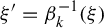. Then $d_{P}(0,\xi ')\leq \delta _0+L+1$ . By the induction hypothesis, there exist $\alpha _1,\ldots ,\alpha _n\in \mathcal {G}$ , with $n\leq KL+N_0$ and ${\xi '\in \alpha _1\ldots \alpha _n(D)}$ . Hence,

$$ \begin{align*}\xi=\beta_k(\xi')\in\beta_k\alpha_1\ldots\alpha_n(D)=\alpha_{1,k}\ldots\alpha_{\ell_k,k}\alpha_1\ldots\alpha_n(D),\end{align*} $$

with $n+\ell _k\leq K(L+1)+N_0$ , since $\ell _k\leq K$ by definition of $K$ . The induction is complete.

Finally, consider $\delta \in (0,K^{-1})$ and $N\in \mathbb {N}$ sufficiently large. Let $\xi \in \mathbb {D}_{(K^{-1}-\delta )N}$ , and define $L=\lceil N(K^{-1}-\delta )-(\delta _0+1)\rceil $ . Recall that $\lceil x\rceil $ denotes the smallest integer ${n\in \mathbb {Z}}$ such that $n\geq x$ , for $x\in \mathbb {R}$ . Applying the result of the previous paragraph, we obtain $\alpha _1,\ldots ,\alpha _n\in \mathcal {G}$ , $n\leq KL+N_0$ , such that $\xi \in \alpha _1\ldots \alpha _n(D)$ . So, it is enough to show that if $N$ is sufficiently large, $KL+N_0\leq N$ . By minimality of $L$ , we have

$$ \begin{align*}KL+N_0\leq K(N(K^{-1}-\delta)-\delta_0)+N_0\leq N-KN\delta+N_0\leq N,\end{align*} $$

if $N\geq N_0K^{-1}\delta ^{-1}$ . This completes the proof.

4 Comparing entropies

4.1 Entropy of a homeomorphisms representation with weighted generators

Here, we consider the abstract setup of a compact metric space $(T,d_T)$ , a group $\mathcal {H}$ , with a (typically finite) set of generators $\mathcal {G}$ such that $\mathcal {G}=\mathcal {G}^{-1}$ , and a morphism $\rho \colon \mathcal {H}\to \operatorname {\mathrm {Homeo}}(T)$ . We will construct some quantity that generalizes slightly an entropy defined by Ghys, Langevin and Walczak [Reference Ghys, Langevin and Walczak21, §2] in this setup.

Consider also $\omega \colon \mathcal {G}\to \mathbb {R}_+^*$ a weight function. Define the Bowen distance for $R>0$ and $t,s\in T$ to be

$$ \begin{align*}d_R^{\rho,\mathcal{G},\omega}(t,s)=\sup\{d_T(\rho(g_1\ldots g_k)(t),\rho(g_1\ldots g_k)(s))\},\end{align*} $$

where the $\sup $ is taken over $g_i\in \mathcal {G}$ , $i\in {[\![} 1,k{]\!]} $ , such that $\sum _{i=1}^k\omega (g_i)\leq R$ , for any $k\in \mathbb {N}$ .

Given such a Bowen distance, we can mimic the vocabulary of §2.2 (see Remark 2.6) for $(R,\varepsilon )$ -covering, dense and separated subsets for $(\rho ,\mathcal {G},\omega )$ . Denote by $B_R^{\rho ,\mathcal {G},\omega }(t,\varepsilon )$ the Bowen ball $\{s\in T;~d_R^{\rho ,\mathcal {G},\omega }(t,s)<\varepsilon \}$ , for $t\in X$ and $R,\varepsilon>0$ . Let $R,\varepsilon>0$ and $Y\subset T$ . Define $N(Y,R,\varepsilon ,\rho ,\mathcal {G},\omega )$ (respectively, $N'(Y,R,\varepsilon ,\rho ,\mathcal {G},\omega )$ ) to be the minimal cardinality of an $(R,\varepsilon )$ -covering subset of $Y$ (respectively, dense subset in $Y$ ), and $M(Y,R,\varepsilon ,\rho ,\mathcal {G},\omega )$ the maximal cardinality of an $(R,\varepsilon )$ -separated subset in $Y$ . With exactly the same proof, we have the same property as Lemma 2.3. Hence, define the entropy of $\rho $ with respect to the set of generators $\mathcal {G}$ and weight $\omega $ by

$$ \begin{align*}h(Y,\rho,\mathcal{G},\omega)=\sup\limits_{\varepsilon>0}\limsup\limits_{R\to +\infty}\frac{1}{R}\log N(Y,R,\varepsilon,\rho,\mathcal{G},\omega).\end{align*} $$ h left parenthesis upper Y comma rho comma script upper G comma omega right parenthesis equals sup Underscript epsilon greater than 0 Endscripts limit sup Underscript upper R right arrow plus infinity Endscripts StartFraction 1 Over upper R EndFraction log upper N left parenthesis upper Y comma upper R comma epsilon comma rho comma script upper G comma omega right parenthesis period

Of course, such a definition would yield the same result if we took $N'(Y,R,\varepsilon ,\rho ,\mathcal {G},\omega )$ or $M(Y,R,\varepsilon ,\rho ,\mathcal {G},\omega )$ instead. If $Y=T$ , denote it simply by $h(\rho ,\mathcal {G},\omega )$ .

Remark 4.1. Let us make a comparison with the similar definition of Ghys, Langevin and Walczak [Reference Ghys, Langevin and Walczak21, §2]. They define the same kind of entropy (without making the Bowen distance explicit) for pseudo-groups of homeomorphisms. Here, we do not need pseudo-groups, since the holonomies of suspensions are global. However, we prefer to define it at the level of representations and not at the level of groups, since we will consider contexts in which two generators have the same image but not the same weight.

Let us denote by $h_{\mathrm {{GLW}}}(\rho (\mathcal {H}),\rho (\mathcal {G}))$ the entropy defined by Ghys. Langevin and Walczak. For reasons of clarity, they need to include the identity in $\mathcal {G}$ but we ignore this issue (or we add it to our setup with $\omega (\operatorname {\mathrm {id}})=0$ ). Our entropy generalizes theirs in the sense that if $1$ denotes the constant weight equal to $1$ , then $h_{\mathrm {{GLW}}}(\rho (\mathcal {H}),\rho (\mathcal {G}))=h(\rho ,\mathcal {G},1)$ . More generally, we have the following lemma.

Lemma 4.2. Retain the notation above. If $c_1\leq \omega \leq c_2$ , for $c_1,c_2\in \mathbb {R}_+^*$ (this always happens for some $c_1,c_2\in \mathbb {R}_+^*$ if $\mathcal {G}$ is finite), then

$$ \begin{align*}c_2^{-1}h_{\mathrm{{GLW}}}(\rho(\mathcal{H}),\rho(\mathcal{G}))\leq h(\rho,\mathcal{G},\omega)\leq c_1^{-1}h_{\mathrm{{GLW}}}(\rho(\mathcal{H}),\rho(\mathcal{G})).\end{align*} $$

Proof. It follows from the definition of $d_R^{\rho ,\mathcal {G},\omega }$ that $d_{c_2^{-1}R}^{\rho ,\mathcal {G},1}\leq d_R^{\rho ,\mathcal {G},\omega }\leq d_{c_1^{-1}R}^{\rho ,\mathcal {G},1}$ . Then separated (respectively, covering) sets for $d_R^{\rho ,\mathcal {G},\omega }$ being separated (respectively, covering) for $d_{c_1^{-1}R}^{\rho ,\mathcal {G},\omega }$ (respectively, $d_{c_2^{-1}R}^{\rho ,\mathcal {G},\omega }$ ), we obtain

$$ \begin{align*} N(Y,c_2^{-1}R,\varepsilon,\rho,\mathcal{G},1)&\leq N(Y,R,\varepsilon,\rho,\mathcal{G},\omega), \\M(Y,R,\varepsilon,\rho,\mathcal{G},\omega)&\leq M(Y,c_1^{-1}R,\varepsilon,\rho,\mathcal{G},1). \end{align*} $$

Taking logarithms, dividing by $R$ and taking the relevant limits, we obtain

$$ \begin{align*}c_2^{-1}h(Y,\rho,\mathcal{G},1)\leq h(Y,\rho,\mathcal{G},\omega)\leq c_1^{-1}h(Y,\rho,\mathcal{G},1).\end{align*} $$

We finish the proof by applying Remark 4.1.

Having proven that our entropy is linked to that of the three authors, we refer the reader to their article [Reference Ghys, Langevin and Walczak21] for examples, estimates, and links to other notions of entropy.

4.2 Entropy of the distinguished transversal

Henceforth, fix $\mathscr {F}=(X,\mathscr {L}){}$ a lamination given by the suspension process of §2.3. Retain the notation introduced there. Also, denote by $D$ a compact fundamental domain of $\Gamma $ , with $0\in D$ , as was done in §3.2 and denote by $\delta _0$ the diameter of $D$ . Moreover, consider a smooth Riemannian metric $g_{M}$ on $X$ , which restricts to a Hermitian metric on the leaves, as explained in §2.1. Denote by $d$ the distance on $X$ induced by $g_{M}$ . We want to reduce the problem of computing the entropy to the distinguished transversal $\mathbb {T}_0$ . More precisely, we first want to obtain the following result.

Theorem 4.3. With the notation above, $h(\mathscr {F})=h(\mathbb {T}_0)+2$ .

To prove the latter, we need several lemmas. The first two concern how fast two automorphisms of the disk diverge from each other if they are close in $0$ . The first one comes from our previous work. The formulation is slightly modified for our purposes, but the statement is exactly the one that is proven (with the notation below, because $e^{-R}\leq 1-\vert \xi \vert ^2\leq 2e^{-R}$ , if $R$ is sufficiently large). The second one comes from Dinh, Nguyên and Sibony’s work on the entropy of foliations. A more precise version of it can be found in [Reference Bacher2, Lemma 3.14], but the one here is sufficient for our needs.

Lemma 4.4. [Reference Bacher2, Lemma 3.11]

Let $\varepsilon>0$ be sufficiently small, $\theta \in [-\pi ,\pi ]$ and $\xi \in \mathbb {D}$ be such that $R=d_{P}(0,\xi )$ is sufficiently large.

(1) If $e^{-R}\geq 8\varepsilon ^{-1}\vert\! \sin (\theta /2)\vert $ , then $d_{P}(\xi ,e^{i\theta }\xi )\leq \varepsilon $ .
(2) If $e^{-R}\leq \tfrac 14\varepsilon ^{-1}\vert\! \sin (\theta /2)\vert $ , then $d_{P}(\xi ,e^{i\theta }\xi )\geq \varepsilon $ .

Lemma 4.5. [Reference Dinh, Nguyên and Sibony10, Lemma 3.8]

Let $\varepsilon>0$ be sufficiently small. There exists $A>1$ such that for all $a,b\in \mathbb {D}$ , the following assertions hold.

(1) If $d_{P}(a,b)\leq A^{-1}e^{-R}$ , then there exist $\tau _a,\tau _b\in \operatorname {\mathrm {Aut}}(\mathbb {D})$ such that $\tau _a(0)=a$ , ${\tau _b(0)=b}$ and $d_{P,\overline {\mathbb {D}}_{R}}(\tau _a,\tau _b)\leq \varepsilon $ .
(2) If $d_{P}(a,b)\geq Ae^{-R}$ , then for all $\tau _a,\tau _b\in \operatorname {\mathrm {Aut}}(\mathbb {D})$ such that $\tau _a(0)=a$ and $\tau _b(0)=b$ , $d_{P,\overline {\mathbb {D}}_{R}}(\tau _a,\tau _b)\geq \varepsilon $ .

Recall the notation

$$ \begin{align*}d_{P,K}(\tau,\sigma)=\sup_{\xi\in K}\,d_{P}(\tau(\xi),\sigma(\xi)),\end{align*} $$

for $K\subset \mathbb {D}$ and $\tau ,\sigma \in \operatorname {\mathrm {Aut}}(\mathbb {D})$ .

We now also need a simple result which compares the Poincaré metric on the disk and on close points in $S$ . Recall the notation $\phi _t$ , for $t\in \mathbb {T}_0$ , introduced in (2.5).

Lemma 4.6. There exist $h>0$ and $c>1$ such that:

(1) if $t\in \mathbb {T}_0$ and $\zeta ,\xi \in \mathbb {D}$ , then $d(\phi _t(\zeta ),\phi _t(\xi ))\leq cd_{P}(\zeta ,\xi )$ ;
(2) if $t,s\in \mathbb {T}_0$ and $\zeta ,\xi \in \mathbb {D}$ are such that $d_{P}(\zeta ,\xi )\leq h$ , then we have $d(\phi _t(\zeta ),\phi _s(\xi ))\geq c^{-1}d_{P}(\zeta ,\xi )$ .

Proof. Note that $\phi _t(\zeta )=\phi _{t'}(\zeta ')$ , for some $\zeta '\in D$ and $t'\in \mathbb {T}_0$ . Then statement (1) follows immediately from the equivalence of Hermitian metrics (2.2) and a compactness argument. For statement (2), let us choose $h>0$ such that

(4.1) $$ \begin{align}d_{P}(\xi,\alpha(\xi))>2h,\quad\xi\in\mathbb{D},\alpha\in\Gamma\setminus\{\operatorname{\mathrm{id}}\}.\end{align} $$

It is classical that such an $h$ exists, since $\Gamma $ is cocompact and since each $\alpha \in \Gamma \setminus \{\operatorname {\mathrm {id}}\}$ has no fixed point. Reducing $h$ if necessary, it is sufficient to prove the statement only for $\phi _t(\zeta )$ and $\phi _s(\xi )$ belonging to a common chart $U\simeq \mathbb {D}\times \mathbb {B}^p$ of the ambient Riemannian manifold $M$ , where $\mathbb {B}^p$ is the unit ball of some $\mathbb {R}^p$ . Take a Riemannian geodesic joining $\phi _t(\zeta )$ and $\phi _s(\xi )$ . If $h$ is sufficiently small, it stays inside $U$ and its projection in the leafwise direction joins $\zeta $ to some $\alpha (\xi )$ , $\alpha \in \Gamma $ . So that it is of Poincaré length at least $d_{P}(\zeta ,\xi )$ , thanks to condition (4.1). We conclude, by compactness of $D\times \mathbb {T}_0$ , the equivalence of Riemannian metrics and (2.2).

The following result will be the last in our preparation for Theorem 4.3, and will still be very useful in the next subsection (see Remark 4.8).

Lemma 4.7. Let $h>0$ be given by Lemma 4.6 and $\delta>0$ . For all $\varepsilon>0$ sufficiently small, and all $R>0$ sufficiently large, we have the following inequality. Let $\zeta \in \mathbb {D}_{h}$ and $t,s\in \mathbb {T}_0$ be such that $d_R(\phi _t(\zeta ),\phi _s(\zeta ))<\varepsilon $ . Then

$$ \begin{align*}d_{\overline{\mathbb{D}}_{(1-\delta)R}}(\phi_t,\phi_s)<2\varepsilon.\end{align*} $$

Here again and in the proof below, we use the notation

$$ \begin{align*}d_{K}(\phi,\psi)=\sup_{\xi\in K}\,d(\phi(\xi),\psi(\xi)),\end{align*} $$

for $K\subset \mathbb {D}$ and $\phi ,\psi \colon \mathbb {D}\to X$ .

Proof. Let $\tau \in \operatorname {\mathrm {Aut}}(\mathbb {D})$ be such that $\tau (0)=\zeta $ and define $\psi _t=\phi _t\circ \tau $ , $\psi _s=\phi _s\circ \tau $ . Since $d_R(\psi _t(0),\psi _s(0))<\varepsilon $ , one finds $\theta \in [-\pi ,\pi ]$ with $d_{\overline {\mathbb {D}}_{R}}(\psi _t,\psi _s\circ r_{\theta })<\varepsilon $ , where $r_{\theta }$ is the rotation of angle $\theta $ in $\mathbb {D}$ . We first show that $\vert \theta \vert \leq e^{-R}$ . Note that if there is some $\xi \in \overline {\mathbb {D}}_{R}$ with $d_{P}(\xi ,e^{i\theta }\xi )\geq c\varepsilon $ , then by continuity, there is a $\xi \in \overline {\mathbb {D}}_{R}$ such that ${h\geq d_{P}(\xi ,e^{i\theta }\xi )\geq c\varepsilon }$ . Applying statement (2) of Lemma 4.6 to $\tau (\xi )$ and $\tau (e^{i\theta }\xi )$ , it follows that $d(\psi _t(\xi ),\psi _s(e^{i\theta }\xi ))\geq \varepsilon $ , a contradiction. Hence, for all $\xi \in \overline {\mathbb {D}}_{R}$ , ${d_{P}(\xi ,e^{i\theta }\xi )\leq c\varepsilon }$ . By statement (2) of Lemma 4.4, one obtains $\vert\! \sin (\theta /2)\vert \leq 4\varepsilon e^{-R}$ , so that $\vert \theta \vert \leq e^{-R}$ , for $\varepsilon $ sufficiently small.

Now, since $\overline {\mathbb {D}}_{(1-\delta )R}\subset \tau (\overline {\mathbb {D}}_{(1-\delta /2)R})$ , for $R$ sufficiently large,

$$ \begin{align*}d_{\overline{\mathbb{D}}_{(1-\delta)R}}(\phi_t,\phi_s)\leq d_{\overline{\mathbb{D}}_{(1-\delta/2)R}}(\psi_t,\psi_s)\leq d_{\overline{\mathbb{D}}_{R}}(\psi_t,\psi_s\circ r_{\theta})+d_{\overline{\mathbb{D}}_{(1-\delta/2)R}}(\psi_s,\psi_s\circ r_{\theta}).\end{align*} $$

Above, the first term of the right-hand side is at most $\varepsilon $ , and the second also by statement (1) of Lemma 4.4. This concludes the proof.

Proof of Theorem 4.3.

We prove the two inequalities separately. Let us first show that $h(\mathscr {F})\leq 2+h(\mathbb {T}_0)$ . Take $F$ an $(R+\delta _0,{\varepsilon }/{2})$ -dense subset in $\mathbb {T}_0$ of minimal cardinality and $G$ an $A^{-1}e^{-R}$ -dense subset of $\mathbb {D}_{\delta _0}$ for the Poincaré distance of minimal cardinality. Here, $A$ is the constant of Lemma 4.5. Define $H=\{\phi _t(\zeta );~t\in F,~\zeta \in G\}$ . We claim that $H$ is $(R,\varepsilon )$ -dense in $X$ . Let $x=\phi _s(\xi )\in X$ , for $s\in \mathbb {T}_0$ and $\xi \in D$ . Take $t\in F$ with $d_{R+\delta _0}(t,s)<{\varepsilon }/{2}$ . In particular, one finds $\theta \in \mathbb {R}$ with $d_{\overline {\mathbb {D}}_{R+\delta _0}}(\phi _t,\phi _s\circ r_{\theta })<{\varepsilon }/{2}$ . Let $\tau $ be an automorphism of the disk satisfying $\tau (0)=e^{-i\theta }\xi $ . Since ${d_{P}(0,\xi )\leq \delta _0}$ , $d_{\overline {\mathbb {D}}_{R}}(\phi _t\circ \tau ,\phi _s\circ r_{\theta }\circ \tau )<{\varepsilon }/{2}$ . Moreover, one can find some $\zeta \in G$ such that we have $d_{P}(\zeta ,\tau (0))<A^{-1}e^{-R}$ , and an automorphism $\sigma $ of $\mathbb {D}$ such that we have $\sigma (0)=\zeta $ and $d_{P,\overline {\mathbb {D}}_{R}}(\sigma ,\tau )\leq c^{-1}({\varepsilon }/{2})$ , by statement (1) of Lemma 4.5. Putting everything together, we obtain

$$ \begin{align*}d_R(x,\phi_t(\zeta))& \leq d_{\overline{\mathbb{D}}_{R}}(\phi_s\circ r_{\theta}\circ\tau,\phi_t\circ\sigma)\\ & \leq d_{\overline{\mathbb{D}}_{R}}(\phi_s\circ r_{\theta}\circ\tau,\phi_t\circ\tau)+d_{\overline{\mathbb{D}}_{R}}(\phi_t\circ\tau,\phi_t\circ\sigma).\end{align*} $$

On the right-hand side, the first term is smaller than ${\varepsilon }/{2}$ , and the second too, by statement (1) of Lemma 4.6. It follows that $H$ is $(R,\varepsilon )$ -dense in $X$ . Hence,

$$ \begin{align*}N'(X,R,\varepsilon)\leq\operatorname{\mathrm{card}}(H)=\operatorname{\mathrm{card}}(F)\operatorname{\mathrm{card}}(G)\leq Ce^{2R}N'\bigg(\mathbb{T}_0,R+\delta_0,\frac{\varepsilon}{2}\bigg).\end{align*} $$

Taking $({1}/{R})\log $ and relevant limits, we obtain $h(\mathscr {F})\leq 2+h(\mathbb {T}_0)$ .

For the other inequality, fix $\delta>0$ , $F$ a $((1-\delta )R,2\varepsilon )$ -separated subset in $\mathbb {T}_0$ of maximal cardinality and $G$ an $Ae^{-R}$ -separated subset for the Poincaré distance in $\mathbb {D}_{h/2}$ of maximal cardinality. Let us show that $H=\{\phi _t(\zeta );~t\in F,~\zeta \in G\}$ is $(R,\varepsilon )$ -separated in $X$ . Take $t,s\in F$ and $\zeta ,\xi \in G$ such that $d_R(\phi _t(\zeta ),\phi _s(\xi ))<\varepsilon $ . We need to prove that $t=s$ , $\zeta =\xi $ . Since $d_R(\phi _t(\zeta ),\phi _s(\xi ))<\varepsilon $ , one finds two automorphisms $\tau ,\sigma \in \operatorname {\mathrm {Aut}}(\mathbb {D})$ such that $\tau (0)=\zeta $ , $\sigma (0)=\xi $ and $d_{\overline {\mathbb {D}}_{R}}(\phi _t\circ \tau ,\phi _s\circ \sigma )<\varepsilon $ . By the same argument as in Lemma 4.7, since $d_{P}(\zeta ,\xi )\leq h$ , it follows that $d_{P,\overline {\mathbb {D}}_{R}}(\tau ,\sigma )\leq c\varepsilon $ . Choosing $A$ above to apply Lemma 4.5(2), one obtains that $d_{P}(\zeta ,\xi )\leq Ae^{-R}$ and that $\zeta =\xi $ , since they both belong to $G$ . Now, apply Lemma 4.7 to obtain that $d_{\overline {\mathbb {D}}_{(1-\delta )R}}(\phi _t,\phi _s)<2\varepsilon $ . Since $t,s\in F$ , one obtains that $t=s$ . Hence, $H$ is $(R,\varepsilon )$ -separated in $X$ and

$$ \begin{align*}M(X,R,\varepsilon)\geq\operatorname{\mathrm{card}}(H)=\operatorname{\mathrm{card}}(F)\operatorname{\mathrm{card}}(G)\geq C^{-1}e^{2R}M(\mathbb{T}_0,(1-\delta)R,2\varepsilon).\end{align*} $$

Taking $({1}/{R})\log $ and limits, one obtains $h(\mathscr {F})\geq 2+(1-\delta )h(\mathbb {T}_0)$ , and since $\delta $ is arbitrary, this concludes the proof.

Remark 4.8. Lemma 4.7 will be very useful in the next subsection, since it will help us to get rid of reparametrization in (2.3) to compute $h(\mathbb {T}_0)$ . Indeed, define another Bowen distance to be, for $R>0$ ,

(4.2) $$ \begin{align}d_R'(t,s)=\sup_{\xi\in\overline{\mathbb{D}}_{R}}\,d(\phi_t(\xi),\phi_s(\xi)),\quad t,s\in\mathbb{T}_0.\end{align} $$

Compared to $d_R$ , instead of being the distance between the two closest parametrizations of $L_{t}$ , $L_{s}$ , this is the distance between the two canonical parametrizations $\phi _t$ of $L_{t}$ and $\phi _s$ of $L_{s}$ . Given the Bowen distance $d_R'$ , we define completely analogous concepts of being $(R,\varepsilon )'$ -covering, dense or separated, for subsets of $\mathbb {T}_0$ . Also, adding primes in the definition, we obtain an analogous notion of entropy denoted by $h'(Y)$ , for $Y\subset \mathbb {T}_0$ .

In fact, $h(Y)=h'(Y)$ . Indeed, it is clear that $d_R'\geq d_R$ . Therefore, $h'(Y)\geq h(Y)$ . On the other hand, Lemma 4.7 gives that, for $\delta>0$ , there is a $C>0$ such that ${d_{(1-\delta )R}'\leq Cd_R}$ , for $R$ sufficiently large. It follows that $h(Y)\geq (1-\delta )h'(Y)$ and, since $\delta $ is arbitrary, $h(Y)=h'(Y)$ . It will be much more convenient to work with $d_R'$ in the following to avoid reparametrization issues. Here, we showed that we are still computing the same entropy.

4.3 Comparing with the weighted entropy

The results of the previous subsection are very general to non-singular laminations (see also [Reference Dinh, Nguyên and Sibony11, Proposition 4.1] for the singular case) and do not really depend on the suspension structure, with minor changes. What should be changed is that we would no longer consider the global transversal $\mathbb {T}_0$ but the union of local transversals in flow boxes. Also, there would be nothing like Lemma 4.7 since there would be no canonical parametrization. In this subsection, we enter more deeply into the structure of a suspension, and into the underlying Fuchsian group.

For $R>0$ , denote $\Gamma _R=\{\alpha \in \Gamma ;~d_{P}(0,\alpha (0))\leq R\}$ , and for $t,s\in \mathbb {T}_0$ , consider yet another Bowen-like distance

(4.3) $$ \begin{align}d_{\Gamma_R}(t,s)=\max\{d(\phi_t(\alpha(0)),\phi_s(\alpha(0)));~\alpha\in\Gamma_R\}.\end{align} $$

This distance is somehow equivalent to the distance $d_R'$ defined in (4.2), in the sense of the following lemma.

Lemma 4.9. For $t,s\in \mathbb {T}_0$ and $R>0$ , we have $d_{\Gamma _R}(t,s)\leq d_R'(t,s)$ . Moreover, for any $\varepsilon>0$ , there exists $\unicode{x3bb}>0$ , independent of $R$ , $t$ and $s$ , such that $d_{\Gamma _{R+\delta _0}}(t,s)\leq \unicode{x3bb} $ implies $d_R'(t,s)\leq \varepsilon $ .

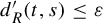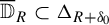
Proof. The first inequality is immediate. For the second, define $\Delta _R=\bigcup _{\alpha \in \Gamma _R}\alpha (\overline {\mathbb {D}}_{\delta _0})$ . Then $\overline {\mathbb {D}}_{R}\subset \Delta _{R+\delta _0}$ . Hence, for $t,s\in \mathbb {T}_0$ ,

(4.4) $$ \begin{align} d_R'(t,s)=d_{\overline{\mathbb{D}}_{R}}(\phi_t,\phi_s)\leq d_{\Delta_{R+\delta_0}}(\phi_t,\phi_s)& \leq\max_{\alpha\in\Gamma_{R+\delta_0}}d_{\overline{\mathbb{D}}_{\delta_0}}(\phi_t\circ\alpha,\phi_s\circ\alpha), \nonumber\\ & \leq \max_{\alpha\in\Gamma_{R+\delta_0}}d^{\prime}_{\delta_0}(\rho(\alpha)(t),\rho(\alpha)(s)).\end{align} $$

StartLayout 1st Row 1st Column d prime Subscript upper R Baseline left parenthesis t comma s right parenthesis equals d Subscript double struck upper D overbar Sub Subscript upper R Baseline left parenthesis phi Subscript t Baseline comma phi Subscript s Baseline right parenthesis less than or equals d Subscript normal upper Delta Sub Subscript upper R plus delta 0 Baseline left parenthesis phi Subscript t Baseline comma phi Subscript s Baseline right parenthesis 2nd Column less than or equals max Underscript alpha element of normal upper Gamma Subscript upper R plus delta 0 Baseline Endscripts d Subscript double struck upper D overbar Sub Subscript delta 0 Subscript Baseline left parenthesis phi Subscript t Baseline ring alpha comma phi Subscript s Baseline ring alpha right parenthesis comma 2nd Row 1st Column Blank 2nd Column less than or equals max Underscript alpha element of normal upper Gamma Subscript upper R plus delta 0 Baseline Endscripts d prime Subscript delta 0 Baseline left parenthesis rho left parenthesis alpha right parenthesis left parenthesis t right parenthesis comma rho left parenthesis alpha right parenthesis left parenthesis s right parenthesis right parenthesis period EndLayout

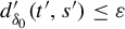
The function $d^{\prime }_{\delta _0}$ is uniformly continuous on the compact $\mathbb {T}_0\times \mathbb {T}_0$ . So, for $\varepsilon>0$ , we can find $\unicode{x3bb}>0$ such that $d(t',s')\leq \unicode{x3bb} $ implies $d^{\prime }_{\delta _0}(t',s')\leq \varepsilon $ , $t',s'\in \mathbb {T}_0$ . Suppose now that $d_{\Gamma _{R+\delta _0}}(t,s)\leq \unicode{x3bb} $ . Then, for all $\alpha \in \Gamma _{R+\delta _0}$ , $d(\rho (\alpha )(t),\rho (\alpha )(s))\leq \unicode{x3bb} $ and thus $d^{\prime }_{\delta _0}(\rho (\alpha )(t),\rho (\alpha )(s))\leq \varepsilon $ . It follows from (4.4) that $d_R'(t,s)\leq \varepsilon $ , as expected.

The previous lemma will enable us to compare the entropy of $\mathscr {F}$ to some weighted entropy for $\Gamma $ and $\rho $ , in the sense of §4.1. Consider $\mathcal {G}$ a set of generators such that $\mathcal {G}=\mathcal {G}^{-1}$ , and for $\alpha \in \mathcal {G}$ , define $\omega (\alpha )=d_{P}(0,\alpha (0))$ . Note that the weight $\omega $ depends only on the Fuchsian group, and not on the representation $\rho $ .

Theorem 4.10. With the notation above, there exists a constant $K'=K'(\Gamma )$ , depending only on the Fuchsian group $\Gamma $ and not on the representation $\rho $ , such that

$$ \begin{align*}h(\rho,\mathcal{G},\omega)\leq h(\mathbb{T}_0)\leq K'h(\rho,\mathcal{G},\omega).\end{align*} $$

Proof. Here, we use the results of §§3.2 and 4.1. By (3.2) and Lemma 4.9, we have $d_R'\geq d_{\Gamma _R}\geq d_R^{\rho ,\mathcal {G},\omega }$ . Hence, considering an $(R,\varepsilon )'$ -dense subset in $\mathbb {T}_0$ , it is $\varepsilon $ -dense for $d_R^{\rho ,\mathcal {G},\omega }$ and $h(\mathbb {T}_0)=h'(\mathbb {T}_0)\geq h(\rho ,\mathcal {G},\omega )$ , by Remark 4.8.

For the other inequality, by Proposition 3.5, $d_{\Gamma _{(K^{-1}-\delta )N}}\leq d_N^{\rho ,\mathcal {G},1}\leq d_{c_2N}^{\rho ,\mathcal {G},\omega }$ , for a constant $K$ depending only on $\Gamma $ , any $\delta \in (0,K^{-1})$ and $N$ sufficiently large. Here, we used the notation of Lemma 4.2. In particular, $c_2=\max \{\omega (\alpha );~\alpha \in \mathcal {G}\}$ only depends on $\Gamma $ . So, using Lemma 4.9, if $d_{c_2N}^{\rho ,\mathcal {G},\omega }(t,s)\leq \unicode{x3bb} $ , then $d^{\prime }_{(K^{-1}-\delta )N-\delta _0}(t,s)\leq \varepsilon $ . Considering a $\unicode{x3bb} $ -dense subset for $d_{c_2N}^{\rho ,\mathcal {G},\omega }$ , it is $((K^{-1}-\delta )N-\delta _0,\varepsilon )'$ -dense. Taking $({1}/{N})\log $ and limits, we obtain $c_2h(\rho ,\mathcal {G},\omega )\geq (K^{-1}-\delta )h'(\mathbb {T}_0)$ . By Remark 4.8 and since $\delta $ is arbitrary, we obtain $h(\mathbb {T}_0)\leq c_2Kh(\rho ,\mathcal {G},\omega )$ , with $K'=c_2K$ only depending on $\Gamma $ .

4.4 Deriving some consequences

We begin by constructing an example showing that entropy is not a smooth invariant. Consider a complex manifold $T$ and $f\colon T\to T$ to be an automorphism of positive entropy $h(f)$ . Take $\rho \colon \Gamma \to \operatorname {\mathrm {Aut}}(T)$ a representation such that $\rho (\alpha _1)=f$ , and $\rho (\alpha _k)=\operatorname {\mathrm {id}}$ , $k\in {[\![} 2,g{]\!]} $ , $\rho (\beta _k)=\operatorname {\mathrm {id}}$ , for $k\in {[\![} 1,g{]\!]} $ . Here, we used the notation of the representation of Proposition 3.3. For such a representation, Ghys, Langevin and Walczak [Reference Ghys, Langevin and Walczak21, Example 2.2] showed that $h_{\text {GLW}}(\rho (\Gamma ),\rho (\mathcal {G}))=2h(f)$ . Moreover, we also obtain that $h(\rho ,\mathcal {G},\omega )=({1}/({\omega (\alpha _1)}))h_{\text {GLW}}(\rho (\Gamma ),\rho (\mathcal {G}))$ with the arguments of Lemma 4.2. This has the following consequence.

Proposition 4.11. There exist two smoothly diffeomorphic foliations $\mathscr {F}_1$ , $\mathscr {F}_2$ such that $h(\mathscr {F}_1)\neq h(\mathscr {F}_2)$ . In other words, entropy is not a $\mathscr {C}^{\infty }$ -invariant.

Proof. Denote by $\mathscr {F}_1$ , $\mathscr {F}_2$ two suspensions obtained by the process above, with different but group-isomorphic Fuchsian groups $\Gamma _1,\Gamma _2$ , respective generators $\mathcal {G}_1$ , $\mathcal {G}_2$ , and with the same $T$ and $f$ . Denote by $\alpha _{1,j}\in \mathcal {G}_j$ , $j\in \{1,2\}$ , the generator of $\Gamma _j$ sent to $f$ . Since the Riemann surfaces $\Sigma _j=\mathbb {D}/\Gamma _j$ 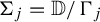are diffeomorphic (being compact and of the same genus) by a diffeomorphism sending $\alpha _{1,1}$ to $\alpha _{1,2}$ , the foliations $\mathscr {F}_1$ and $\mathscr {F}_2$ are diffeomorphic. Moreover, by the paragraph above and by Theorems 4.3 and 4.10,

$$ \begin{align*}\begin{aligned}h(\mathscr{F}_1)&\leq2+K'(\Gamma_1)h(\rho_1,\mathcal{G}_1,\omega_1)=2+2h(f)\frac{K'(\Gamma_1)}{\omega_1(\alpha_{1,1})},\\ h(\mathscr{F}_2)&\geq2+h(\rho_2,\mathcal{G}_2,\omega_2)=2+\frac{2h(f)}{\omega_2(\alpha_{1,2})}.\end{aligned}\end{align*} $$

StartLayout 1st Row StartLayout 1st Row 1st Column h left parenthesis script upper F 1 right parenthesis 2nd Column less than or equals 2 plus upper K prime left parenthesis normal upper Gamma 1 right parenthesis h left parenthesis rho 1 comma script upper G 1 comma omega 1 right parenthesis equals 2 plus 2 h left parenthesis f right parenthesis StartFraction upper K prime left parenthesis normal upper Gamma 1 right parenthesis Over omega 1 left parenthesis alpha Subscript 1 comma 1 Baseline right parenthesis EndFraction comma 2nd Row 1st Column h left parenthesis script upper F 2 right parenthesis 2nd Column greater than or equals 2 plus h left parenthesis rho 2 comma script upper G 2 comma omega 2 right parenthesis equals 2 plus StartFraction 2 h left parenthesis f right parenthesis Over omega 2 left parenthesis alpha Subscript 1 comma 2 Baseline right parenthesis EndFraction period EndLayout EndLayout

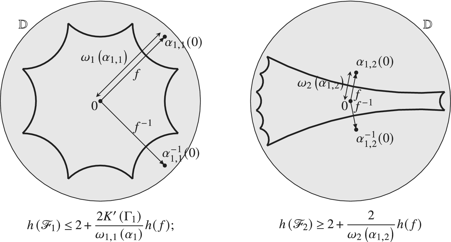
So, fixing $\Gamma _1$ and choosing $\Gamma _2$ in consequence, it is enough to find it, along with a generator $\alpha _{1,2}$ such that $\omega _2(\alpha _{1,2})=d_{P}(0,\alpha _{1,2}(0))<({\omega _1(\alpha _{1,1})}/({K'(\Gamma _1)}))$ , which is a fixed constant. This can be achieved by Proposition 3.4 (see Figure 2). The whole point is that one can find a fixed generator $\alpha _{1,1}\in \mathcal {G}_1$ , which will be sent to the $\alpha _{\varepsilon }$ of Proposition 3.4 by the diffeomorphism. This is guaranteed by the construction of $\alpha _{\varepsilon }$ and by [Reference Farb and Margalit14, 10.4.2].

Remark 4.12. We believe that such a construction can show that there are suspensions for which all values in $(2,\infty )$ can be achieved in their class of diffeomorphism. Indeed, the proof above shows that arbitrarily large entropy can be achieved. Moreover, Proposition 3.4 can be adapted to have a generator of arbitrary large weight. In §5.3, we will even get an exact value of the entropy, of the form $2K_0h(f)$ , with a constant $K_0$ depending only on $\Gamma $ . However, this is not sufficient, since the constant $K_0$ is not easily seen to depend continuously on the Fuchsian group, and we are not able to control it enough to show that arbitrarily small entropy greater than $2$ can be achieved.

Figure 2

Fundamental domains in the proof of Proposition 3.4.

Two-panel mathematical diagram showing fundamental domains within “unit disks D” should be enough. See long description.

Figure 2 Long description

A two-panel diagram illustrating geometric proofs.

Left Panel:

A unit disk D contains a central star-like polygon with eight equal concave sides. At the center is a point labeled 0. A double-headed arrow labeled f connects point 0 to an external point alpha sub 1,1 (0). This arrow has weight omega sub 1 (alpha sub 1,1). A single-headed arrow labeled f super -1 points from the center toward a point alpha sub 1,1 super -1 (0) located outside the polygon. Below the disk is the inequality: h (script F sub 1) is less than or equal to 2 plus the fraction 2 K prime (Gamma sub 1) over omega sub 1,1 (alpha sub 1) times h (f).

Right Panel:

A unit disk D contains a horizontal, trumpet-shaped domain that narrows toward the right. The center point 0 is located within this domain. A short double-headed arrow labeled f connects point 0 to an external point alpha sub 1,2 (0) above the domain. A single-headed arrow labeled f super -1 points from the center to a point alpha sub 1,2 super -1 (0) below the domain. These arrows have weight omega sub 2 (alpha sub 1,2). Below the disk is the inequality: h (script F sub 2) is greater than or equal to 2 plus the fraction 2 over omega sub 2 (alpha sub 1,2) times h (f).

So, the entropy is not a smooth invariant. However, in the case of suspensions and of homeomorphisms like that in the proof of Proposition 4.11, we have the following proposition.

Proposition 4.13. Let $\Phi \colon \Sigma _1\to \Sigma _2$ be a homeomorphism between two hyperbolic Riemann surfaces inducing an isomorphism $\varphi \colon \Gamma _1=\pi _1(\Sigma _1)\to \Gamma _2=\pi _1(\Sigma _2)$ , let ${\Psi \colon T_1\to T_2}$ a homeomorphism between compact metric spaces, and for $i\in\{1,2\}$ , let $\rho _i\colon \Gamma _i\to \operatorname {\mathrm {Homeo}}(T_i)$ , $i\in \{1,2\}$ , be representations satisfying the conjugacy $\rho _2(\gamma _2)=\Psi \circ \rho _1(\varphi ^{-1}(\gamma _2))\circ \Psi ^{-1}$ , for $\gamma _2\in \Gamma _1$ .

Let $\mathscr {F}_i$ be the usual suspension of the representation $\rho _i$ , $i\in \{1,2\}$ . Then $h(\mathscr {F}_1)=2$ if and only if $h(\mathscr {F}_2)=2$ , and $h(\mathscr {F}_1)=+\infty $ if and only if $h(\mathscr {F}_2)=+\infty $ .

Proof. By Theorems 4.3 and 4.10, we have $h(\mathscr {F}_i)=2$ (respectively, $h(\mathscr {F}_i)=+\infty $ ) if and only if $h_{\text {GLW}}(\rho _i(\Gamma _i),\rho _i(\mathcal {G}_i))=0$ (respectively, $=+\infty $ ), for $i\in \{1,2\}$ . Since $\Psi $ is uniformly continuous, it is easy to obtain the statement of the proposition from this observation.

It is worth noting that having infinite entropy is quite a wild phenomenon. Indeed, for a general compact lamination, it was shown by Dinh, Nguyên and Sibony (see [Reference Dinh, Nguyên and Sibony10]) that if it is of class $\mathscr {C}^{2+\alpha }$ , for $\alpha>0$ , then it has finite entropy. In the case of suspensions, thanks to a result of Ghys, Langevin and Walczak, one can do better.

Proposition 4.14. Let $\mathscr {F}$ be a Lipschitz suspension. Then $h(\mathscr {F})<+\infty $ .

Proof. We use the notation of the previous subsection. If $\rho (\mathcal {G})$ contains only Lipschitz maps, it follows from [Reference Ghys, Langevin and Walczak21, Proposition 2.7] that $h_{\text {GLW}}(\rho (\Gamma ),\rho (\mathcal {G}))$ is finite. We apply Theorem 4.10 and Lemma 4.2 to conclude the proof.

On the other hand, still by previous work of Ghys, Langevin and Walczak, we have the following necessary condition for having minimal entropy $2$ . Note that a priori, having an invariant measure for the action of a non-amenable group $\Gamma $ is a rare phenomenon (see, for example, [Reference Cantat and Dujardin8, Reference Furman18, Reference Roda33] and references therein).

Proposition 4.15. Let $\mathscr {F}$ be a suspension with entropy $2$ . Then there exists a Borel probability measure $\nu $ on $T$ which is invariant by $\Gamma $ (see Definition 5.2).

Proof. It is shown in [Reference Ghys, Langevin and Walczak21, §5] that if $\Gamma $ is a group of homeomorphisms of a compact metric space $T$ and $\mathcal {G}$ is a set of generators of $\Gamma $ such that $\mathcal {G}=\mathcal {G}^{-1}$ and ${h_{\text {GLW}}(\Gamma ,\mathcal {G})=0}$ , then there exists a probability measure $\nu $ on $T$ which is invariant by $\Gamma $ . Since by Theorem 4.10 and Lemma 4.2, $h(\mathscr {F})\geq 2+c_2h_{\text {GLW}}(\rho (\Gamma ),\rho (\mathcal {G}))$ , for $c_2=\max (\omega )$ , this result applies.

5 Measure-theoretic entropy

In this section, we consider a measure-theoretic entropy for hyperbolic laminations, defined by Dinh, Nguyên and Sibony [Reference Dinh, Nguyên and Sibony10].

5.1 Harmonic, invariant and stationary measures

Definition 5.1. Roughly speaking, harmonic measures are quasi-invariant measures by the lamination $\mathscr {F}$ . More precisely, let $\mathscr {F}=(X,\mathscr {L})$ be a hyperbolic lamination and $\mu $ be a Borel probability measure on $X$ . The measure $\mu $ is said to be harmonic if, for every flow box $U\simeq \mathbb {D}\times \mathbb {T}$ , there exist a Radon measure $\nu $ on $\mathbb {T}$ and harmonic functions ${h_t\colon \mathbb {D}\to \mathbb {R}_+}$ , for $t\in \mathbb {T}$ , such that for every integrable function $f\colon U\to \mathbb {R}$ ,

(5.1) $$ \begin{align} \int fd\mu=\int_{\mathbb{T}}\int_{\mathbb{D}}h_t(z)f(t,z)g_{P}{}(z)\,d\nu(t).\end{align} $$

If, moreover, the harmonic functions $h_t$ , $t\in \mathbb {T}$ , are all constant, $\mu $ is called an invariant measure.

There are analogous concepts for group actions.

Definition 5.2. Let $\Gamma $ be a group acting on a topological space $T$ and $m$ be a probability measure on $\Gamma $ . A Borel measure $\nu $ on $T$ is called invariant by $\Gamma $ if, for every $\gamma \in \Gamma $ , $\gamma _*\nu =\nu $ . It is called m-stationary if it is invariant on average, that is, if

$$ \begin{align*}\int_{\Gamma}\gamma_*\nu\, dm(\gamma)=\nu.\end{align*} $$

In fact, in the case of suspensions, there is a bridge between these two pairs of notions with the following result.

Theorem 5.3. (Alvarez [Reference Alvarez1])

Let $\Sigma =\mathbb {D}/\Gamma $ be a smooth compact Riemann surface of genus $g\geq 2$ . There exists a probability measure $m$ on $\Gamma $ such that $m(\gamma )>0$ for every $\gamma \in \Gamma $ and satisfying the following assertion. Let $\mathscr {F}$ be a suspension obtained as in §2.3. Then the map

$$ \begin{align*}\mu\mapsto h_t(0)\,d\nu(t),\end{align*} $$

with the notation of (5.1) on the flow box $U\times \mathbb {T}_0$ , for $U$ a small neighborhood of $0$ in $\mathbb {D}$ , sends bijectively harmonic measures for $\mathscr {F}$ onto $m$ -stationary measures for $\Gamma $ . Moreover, it maps bijectively invariant measures for $\mathscr {F}$ onto invariant measures for $\Gamma $ , and bijectively ergodic measures for $\mathscr {F}$ onto ergodic measures for $\Gamma $ .

The theorem above is valid in a broader context, but we state it in the one that is relevant here. Note that Proposition 4.15 now gives the following proposition.

Proposition 5.4. Let $\mathscr {F}$ be a suspension with entropy $2$ . Then there exists an invariant measure for $\mathscr {F}$ .

5.2 Entropy of a harmonic measure

For the dynamics of a single map, the usual definition of the entropy of a measure relies on measurable partitions. In our context, such a definition does not work, but thanks to the Katok [Reference Katok24] and Brin–Katok [Reference Brin and Katok6] theorems, one can still have analogies with only a notion of Bowen balls.

Definition 5.5. [Reference Dinh, Nguyên and Sibony10, §4]

Let $\mathscr {F}=(X,\mathscr {L}){}$ be a hyperbolic lamination and $\mu $ a harmonic measure for $\mathscr {F}$ . For $R,\varepsilon ,\delta>0$ , denote by $N(R,\varepsilon ,\delta )$ the minimal amount of $(R,\varepsilon )$ -Bowen balls required to cover a subset of $\mu $ -measure at least $1-\delta $ . Define the entropy of $\mu $ to be

$$ \begin{align*}h(\mu)=\sup_{\delta>0}\sup_{\varepsilon>0}\limsup_{R\to+\infty}\frac{1}{R}\log N(R,\varepsilon,\delta).\end{align*} $$ h left parenthesis mu right parenthesis equals sup Underscript delta greater than 0 Endscripts sup Underscript epsilon greater than 0 Endscripts limit sup Underscript upper R right arrow plus infinity Endscripts StartFraction 1 Over upper R EndFraction log upper N left parenthesis upper R comma epsilon comma delta right parenthesis period

Given $x\in X$ , one also defines local upper and lower entropies of $\mu $ at $x$ :

$$ \begin{align*}\begin{aligned} h^+(\mu,x)&=\sup_{\varepsilon>0}\limsup_{R\to+\infty}-\frac{1}{R}\log\mu(B_R(x,\varepsilon)),\\ h^-(\mu,x)&=\sup_{\varepsilon>0}\liminf_{R\to+\infty}-\frac{1}{R}\log\mu(B_R(x,\varepsilon)).\end{aligned}\end{align*} $$

StartLayout 1st Row StartLayout 1st Row 1st Column h Superscript plus Baseline left parenthesis mu comma x right parenthesis 2nd Column equals sup Underscript epsilon greater than 0 Endscripts limit sup Underscript upper R right arrow plus infinity Endscripts minus StartFraction 1 Over upper R EndFraction log mu left parenthesis upper B Subscript upper R Baseline left parenthesis x comma epsilon right parenthesis right parenthesis comma 2nd Row 1st Column h Superscript minus Baseline left parenthesis mu comma x right parenthesis 2nd Column equals sup Underscript epsilon greater than 0 Endscripts limit inf Underscript upper R right arrow plus infinity Endscripts minus StartFraction 1 Over upper R EndFraction log mu left parenthesis upper B Subscript upper R Baseline left parenthesis x comma epsilon right parenthesis right parenthesis period EndLayout EndLayout

Finally, consider a local flow box $U\simeq \mathbb {D}\times \mathbb {T}$ and a local disintegration of $\mu $ into a leafwise harmonic density and a transversal Radon measure $\nu $ as in (5.1). Rescale the $h_t$ and $\nu $ if necessary to have that $h_t(0)=1$ , for all $t\in \mathbb {T}$ . Let $\pi _{\mathbb {T}}\colon U\to \mathbb {T}$ be the projection on the second coordinate. Define the local transversal upper and lower entropies of $\mu $ at $x$ to be

$$ \begin{align*}\begin{aligned} \widetilde{h}^+(\mu,x)&=\sup_{\varepsilon>0}\limsup_{R\to+\infty}-\frac{1}{R}\log\nu(\pi_{\mathbb{T}}(B_R(x,\varepsilon))),\\ \widetilde{h}^-(\mu,x)&=\sup_{\varepsilon>0}\liminf_{R\to+\infty}-\frac{1}{R}\log\nu(\pi_{\mathbb{T}}(B_R(x,\varepsilon))).\end{aligned}\end{align*} $$

StartLayout 1st Row StartLayout 1st Row 1st Column ModifyingAbove h With tilde Superscript plus Baseline left parenthesis mu comma x right parenthesis 2nd Column equals sup Underscript epsilon greater than 0 Endscripts limit sup Underscript upper R right arrow plus infinity Endscripts minus StartFraction 1 Over upper R EndFraction log nu left parenthesis pi Subscript double struck upper T Baseline left parenthesis upper B Subscript upper R Baseline left parenthesis x comma epsilon right parenthesis right parenthesis right parenthesis comma 2nd Row 1st Column ModifyingAbove h With tilde Superscript minus Baseline left parenthesis mu comma x right parenthesis 2nd Column equals sup Underscript epsilon greater than 0 Endscripts limit inf Underscript upper R right arrow plus infinity Endscripts minus StartFraction 1 Over upper R EndFraction log nu left parenthesis pi Subscript double struck upper T Baseline left parenthesis upper B Subscript upper R Baseline left parenthesis x comma epsilon right parenthesis right parenthesis right parenthesis period EndLayout EndLayout

In our context, such quantities were studied by Dinh, Nguyên and Sibony [Reference Dinh, Nguyên and Sibony10] (see also [Reference Bacher2] for a singular context). In particular, they show the following theorem.

Theorem 5.6. (Dinh–Nguyên–Sibony [Reference Dinh, Nguyên and Sibony10, Theorem 4.2 and Proposition 4.5])

Consider $\mathscr {F}=(X,\mathscr {L})$ a compact hyperbolic lamination and $\mu $ a harmonic measure. Then the quantities $x\mapsto \widetilde {h}^{\pm }(\mu ,x)$ and $x\mapsto h^{\pm }(\mu ,x)$ are leafwise constant with ${h^{\pm }(\mu ,x)=2+\widetilde {h}^{\pm }(\mu ,x)}$ . In particular, if $\mu $ is ergodic, then all these quantities are constant almost everywhere. Denote them by $\widetilde {h}^{\pm }(\mu )$ , $h^{\pm }(\mu )$ . We have

$$ \begin{align*}2\leq h^-(\mu)\leq h(\mu)\leq h^+(\mu)\leq h(\mathscr{F}).\end{align*} $$

In [Reference Dinh, Nguyên and Sibony10, Problems 5 and 6], the three authors ask whether $h^+(\mu )=h^-(\mu )$ holds (this would be a Brin–Katok-type theorem) and whether one has the variational principle $h(\mathscr {F})=\sup _{\mu }h(\mu )$ . Except when the entropy equals $2$ , for which it is trivial, there are no examples yet in which one can show whether or not it holds. Below, in Theorem 5.8, we will study a toy example in which one can use the classical theorems for maps to show them on foliations.

Before ending this subsection, let us give a more adapted way to compute the transversal entropies in the case of suspensions.

Lemma 5.7. Let $\mathscr {F}$ be a suspension with the usual notation, $\mu $ be a harmonic measure for $\mathscr {F}$ , and recall the Bowen distances $d_R'$ defined in (4.2). For $t\in T$ , define

$$ \begin{align*}B_R^{\mathbb{T}}(t,\varepsilon)=\{s\in T;~d_R'(s,t)<\varepsilon\},\quad B_R^{\mathbb{T},\Gamma}(t,\varepsilon)=\{s\in T;~d_{\Gamma_R}(t,s)<\varepsilon\},\end{align*} $$

where $d_{\Gamma _R}$ is defined in (4.3). Then, if $\nu $ denotes the measure on $T$ given by Theorem 5.3,

$$ \begin{align*}\begin{aligned}\widetilde{h}^+(\mu,t)&=\sup_{\varepsilon>0}\limsup_{R\to+\infty}-\frac{1}{R}\log\nu(B_R^{\mathbb{T}}(t,\varepsilon))=\sup_{\varepsilon>0}\limsup_{R\to+\infty}-\frac{1}{R}\log\nu(B_R^{\mathbb{T},\Gamma}(t,\varepsilon)),\\\widetilde{h}^-(\mu,t)&=\sup_{\varepsilon>0}\liminf_{R\to+\infty}-\frac{1}{R}\log\nu(B_R^{\mathbb{T}}(t,\varepsilon))=\sup_{\varepsilon>0}\liminf_{R\to+\infty}-\frac{1}{R}\log\nu(B_R^{\mathbb{T},\Gamma}(t,\varepsilon)).\end{aligned}\end{align*} $$

StartLayout 1st Row StartLayout 1st Row 1st Column ModifyingAbove h With tilde Superscript plus Baseline left parenthesis mu comma t right parenthesis 2nd Column equals sup Underscript epsilon greater than 0 Endscripts limit sup Underscript upper R right arrow plus infinity Endscripts minus StartFraction 1 Over upper R EndFraction log nu left parenthesis upper B Subscript upper R Superscript double struck upper T Baseline left parenthesis t comma epsilon right parenthesis right parenthesis equals sup Underscript epsilon greater than 0 Endscripts limit sup Underscript upper R right arrow plus infinity Endscripts minus StartFraction 1 Over upper R EndFraction log nu left parenthesis upper B Subscript upper R Superscript double struck upper T comma normal upper Gamma Baseline left parenthesis t comma epsilon right parenthesis right parenthesis comma 2nd Row 1st Column ModifyingAbove h With tilde Superscript minus Baseline left parenthesis mu comma t right parenthesis 2nd Column equals sup Underscript epsilon greater than 0 Endscripts limit inf Underscript upper R right arrow plus infinity Endscripts minus StartFraction 1 Over upper R EndFraction log nu left parenthesis upper B Subscript upper R Superscript double struck upper T Baseline left parenthesis t comma epsilon right parenthesis right parenthesis equals sup Underscript epsilon greater than 0 Endscripts limit inf Underscript upper R right arrow plus infinity Endscripts minus StartFraction 1 Over upper R EndFraction log nu left parenthesis upper B Subscript upper R Superscript double struck upper T comma normal upper Gamma Baseline left parenthesis t comma epsilon right parenthesis right parenthesis period EndLayout EndLayout

Proof. The right equalities are consequences of Lemma 4.9. For the left ones, with the notation of Definition 5.5, for some small $h>0$ and if $\varepsilon $ is sufficiently small,

$$ \begin{align*}\pi_{\mathbb{T}}(B_R(t,\varepsilon))=\{s\in T; \text{ there exists }\zeta\in\mathbb{D}_{h}~\text{with}~d_R(\phi_s(\zeta),t)<\varepsilon\}.\end{align*} $$

Since $d_R'>d_R$ , it is clear that we have the inequality ‘ $\leq $ ’ in the two equalities to be shown. Now consider $s\in \pi _{\mathbb {T}}(B_R(t,\varepsilon ))$ and take $\zeta \in \mathbb {D}_{h}$ with $d_R(\phi _s(\zeta ),t)<\varepsilon $ . By the same arguments as in Lemma 4.7, we have $d_{P}(0,\zeta )<Ae^{-R}$ . It follows by statement (1) of Lemma 4.5 that $d_{R(1-\delta )}(\phi _s(\zeta ),\phi _s(0))<\varepsilon $ , for any $\delta>0$ and $R$ sufficiently large. Hence, $d_{R(1-\delta )}(t,s)<2\varepsilon $ and $d^{\prime }_{R(1-\delta )^2}(s,t)<4\varepsilon $ by Lemma 4.7. We conclude by the same arguments as in Remark 4.8.

5.3 The case of a single map

Here, we consider a suspension $\mathscr {F}$ , for which the image of the representation $\rho (\Gamma )=\langle f\rangle \simeq \mathbb {Z}$ is generated by a single map $f$ , and with the usual notation. More precisely, for $\alpha \in \mathcal {G}$ , denote by $n(\alpha )\in \mathbb {Z}$ the integer such that $\rho (\alpha )=f^{n(\alpha )}$ . Our main result is the following theorem.

Theorem 5.8. In the setup above, there exists a constant $K_0$ that does not depend on $f$ , such that the following assertions hold.

(1) We have $h(\mathscr {F})=2+2K_0h_{\mathrm {top}}(f)$ .
(2) Every harmonic measure $\mu $ on $\mathscr {F}$ is actually invariant. Denote by $\nu $ its trace on $T$ given by Theorem 5.3. Then, if $\mu $ is ergodic,
$$ \begin{align*}h^-(\mu)=h(\mu)=h^+(\mu)=2+2K_0h_{\nu}(f).\end{align*} $$
(3) We have $h(\mathscr {F})=\sup _{\mu }h(\mu )=\sup _{\mu ~\mathrm {ergodic}}h(\mu )$ .

Here, the fact that $K_0$ does not depend on $f$ means more precisely that it depends only on the Fuchsian group $\Gamma $ , and on the powers $n(\alpha )$ , for $\alpha \in \mathcal {G}$ , but not on other choices. Moreover, we denoted by $h_{\mathrm {top}}(f)$ the topological entropy of $f$ in the usual sense, and by $h_{\nu }(f)$ its measure-theoretic entropy for $\nu $ . Note that item (3) is a consequence of the first two, and of the classical variational principle for maps (see [Reference Walters34, Theorem 8.6 and Corollary 8.6.1]). Let us emphasize the $2$ in the theorem above, which comes from the fact that powers of $f$ from $-n$ to $n$ are considered, instead of classically from $0$ to $n$ .

Remark 5.9. Theorem 5.8 shows that there is no converse to Proposition 4.15. Even a weak version stating that $\mu $ invariant implies $h(\mu )=0$ does not hold. Here, even if all harmonic measures are invariant, we do not necessarily have that $h(\mathscr {F})=2$ . Other examples of random dynamical systems for which all stationary measures are invariant (so-called stiffness) can be found in [Reference Cantat and Dujardin8, Reference Roda33] and references therein.

Let us start by finding the constant $K_0$ . For $R>0$ , denote

$$ \begin{align*}n(R)=\max\{n\in\mathbb{N}; \text{ there exists }\alpha\in\Gamma,~d_{P}(0,\alpha(0))\leq R~\text{and}~\rho(\alpha)=f^n\}.\end{align*} $$

Lemma 5.10. The limit $K_0=\lim _{R\to +\infty }(({n(R)})/{R})$ exists in $\mathbb {R}_+^*$ .

Proof. It is easy to see that $R\mapsto -n(R)$ is subadditive. Hence, the limit of ${n(R)}/{R}$ exists in $[0,\infty ]$ by [Reference Walters34, Theorem 4.9]. Moreover, there exists $K_1>1$ with $K_1^{-1}R\leq n(R)\leq K_1R$ , for sufficiently large $R$ . Indeed, on the one hand $n(R)\geq \lfloor {R}/({d_{P}(0,\alpha (0))})\rfloor \vert n(\alpha )\vert $ , for $\alpha \in \mathcal {G}$ . On the other hand, using the notation of Proposition 3.5 and applying it to $\delta =K^{-1}/2$ , one obtains $n(R)\leq \lceil 2KR\rceil \max _{\alpha \in \mathcal {G}}n(\alpha )$ . Therefore, $K_0$ is neither $0$ nor $\infty $ . Recall that for $x\in \mathbb {R}$ , we denote by $\lfloor x\rfloor $ (respectively, $\lceil x\rceil $ ) the highest (respectively, lowest) integer $n\in \mathbb {Z}$ such that $n\leq x$ (respectively, $n\geq x$ ).

Proof of item (1) of Theorem 5.8.

Note that the constant $K_0$ in the lemma above depends only on the Fuchsian group and on the powers $n(\alpha )$ , $\alpha \in \mathcal {G}$ . Now, recall the Bowen distance $d_{\Gamma _R}$ defined in (4.3) and denote $d_n^{f^{\pm 1}}(t,s)=\max _{i\in {[\![} -n,n{]\!]} }d(f^i(s),f^i(s))$ , for $s,t\in T$ and $n\in \mathbb {N}$ . Finally, denote by $d_n^f(s,t)=\max _{i\in {[\![} 0,n{]\!]} }d(f^i(s),f^i(t))$ the classical Bowen distance. Write $B_{\Gamma _R}(t,\varepsilon )$ , $B_n^{f^{\pm 1}}(t,\varepsilon )$ , $B_n^f(t,\varepsilon )$ for the corresponding Bowen balls and $N_{\Gamma }(T,R,\varepsilon )$ , $N_f(T,n,\varepsilon )$ , $N_{f^{\pm 1}}(T,n,\varepsilon )$ for the corresponding minimal number of Bowen balls required to cover $T$ , as in Definition 2.2. Then the Bowen definition of the topological entropy [Reference Walters34, Definitions 7.9 and 7.10] is

$$ \begin{align*}h_{\mathrm{top}}(f)=\sup_{\varepsilon>0}\limsup_{n\to+\infty}\frac{1}{n}\log N_f(T,n,\varepsilon).\end{align*} $$ h Subscript top Baseline left parenthesis f right parenthesis equals sup Underscript epsilon greater than 0 Endscripts limit sup Underscript n right arrow plus infinity Endscripts StartFraction 1 Over n EndFraction log upper N Subscript f Baseline left parenthesis upper T comma n comma epsilon right parenthesis period

On the other hand, for $t\in T$ and $n,\varepsilon>0$ , $B_n^{f^{\pm 1}}(t,\varepsilon )=f^n(B_{2n}^f(f^{-n}(t),\varepsilon ))$ , so that $N_{f^{\pm 1}}(T,n,\varepsilon )=N_f(T,2n,\varepsilon )$ . Now if we define

$$ \begin{align*}I(R)=\{i\in\mathbb{Z}; \text{ there exists }\alpha\in\Gamma,~d_{P}(0,\alpha(0))\leq R,~\rho(\alpha)=f^i\},\end{align*} $$

by definition $I(R)\subset {[\![} -n(R),n(R){]\!]} $ . Moreover, the maximal step between two consecutive points of $I(R)$ is at most $P=\max _{\alpha \in \mathcal {G}}(n(\alpha ))$ . Therefore, by a uniform continuity argument on $f^p$ , for $p\in {[\![} 1,P{]\!]} $ , as in Lemma 4.9, we have that for all $\varepsilon>0$ , there exists $\unicode{x3bb}>0$ such that $B_{\Gamma _R}(t,\unicode{x3bb} )\subset B_{n(R)}^{f^{\pm 1}}(t,\varepsilon )\subset B_{\Gamma _R}(t,\varepsilon )$ , for any $t\in T$ . Hence,

$$ \begin{align*}N_{\Gamma}(\mathbb{T}_0,R,\unicode{x3bb})\geq N_{f^{\pm1}}(T,n(R),\varepsilon)=N_f(T,2n(R),\varepsilon)\geq N_{\Gamma}(\mathbb{T}_0,R,\varepsilon).\end{align*} $$

We conclude with Lemma 5.10, the usual arguments that $d_{\Gamma _R}$ and $d_R$ define the same entropy, and Theorem 4.3.

Note that by the above inclusions, and by Lemma 5.7, we have the following lemma.

Lemma 5.11. With the setup of Theorem 5.8, for $t\in T$ ,

$$ \begin{align*}\begin{aligned} \widetilde{h}^+(\mu,t)&=K_0\sup_{\varepsilon>0}\limsup_{n\to+\infty}\bigg(\!{-}\frac{1}{n}\log\nu\left(B_n^{f^{\pm1}}(t,\varepsilon)\right)\bigg),\\\widetilde{h}^-(\mu,t)&=K_0\sup_{\varepsilon>0}\liminf_{n\to+\infty}\bigg(\!{-}\frac{1}{n}\log\nu\left(B_n^{f^{\pm1}}(t,\varepsilon)\right)\bigg). \end{aligned}\end{align*} $$

By the martingale theorem and the Hewitt–Savage $0$ – $1$ law [Reference Blackwell5], one can show that every bounded $\rho _*m$ -harmonic function on $\mathbb {Z}$ is constant. This is actually a very simple case of the Choquet–Deny property of virtually nilpotent groups [Reference Frisch, Hartman, Tamuz and Ferdowsi17]. In particular, it implies that any $m$ -stationary measure $\nu $ is actually invariant by $f$ . Hence, by Theorems 5.3 and 5.6, the proof of Theorem 5.8 is reduced to the following proposition.

Proposition 5.12. Let $f\colon T\to T$ be a homeomorphism of a compact metric space and $\nu $ be an ergodic invariant measure. Then, for $\nu $ -almost every $t\in T$ ,

$$ \begin{align*}\sup_{\varepsilon>0}\liminf_{n\to+\infty}\left(-\frac{1}{n}\log\nu\left(B_n^{f^{\pm1}}(t,\varepsilon)\right)\right)= \sup_{\varepsilon>0}\limsup_{n\to+\infty}\left(-\frac{1}{n}\log\nu\left(B_n^{f^{\pm1}}(t,\varepsilon)\right)\right)=2h_{\nu}(f).\end{align*} $$

This is almost exactly like the Brin–Katok theorem [Reference Brin and Katok6], except that two-sided Bowen balls $B_n^{f^{\pm 1}}$ are involved, instead of usual Bowen balls $B_n^f$ . Of course, our arguments will use the Brin–Katok theorem and its proof.

Proof. We only do the proof for $h_{\nu }(f)<+\infty $ , since it is easy to adapt it for infinite entropy. Let us start by showing that the $\liminf $ is greater than $2h_{\nu }(f)$ . This is the most complicated part of Brin and Katok’s proof, but they show [Reference Brin and Katok6, pp. 37] that for every $\delta>0$ , there exists $\varepsilon>0$ with

$$ \begin{align*}\left(\nu\left\{t\in T;~\nu\left(B_n^f(t,\varepsilon)\right)>\exp(-(h_{\nu}(f)-\delta)n)\right\}\right)_{n\in\mathbb{N}} \end{align*} $$

summable. Since $\nu (B_n^{f^{\pm 1}}(t,\varepsilon ))=\nu (B_{2n}^f(f^{-n}(t),\varepsilon ))$ because $\nu $ is invariant,

$$ \begin{align*}\left(\nu\left\{t\in T;~\nu\left(B_n^{f^{\pm1}}(t,\varepsilon)\right)>\exp(-2(h_{\nu}(f)-\delta)n)\right\}\right)_{n\in\mathbb{N}}\end{align*} $$

is also summable. Here, we used again the $\nu $ -invariance by $f$ . Just like Brin and Katok, we conclude by the Borel–Cantelli theorem that for $\nu $ -almost every $t\in T$ ,

(5.2) $$ \begin{align}\sup_{\varepsilon>0}\liminf_{n\to+\infty}\left(-\frac{1}{n}\log\nu\left(B_n^{f^{\pm1}}(t,\varepsilon)\right)\right)\geq2h_{\nu}(f).\end{align} $$

Now let us proceed with showing that the $\limsup $ is lower than $2h_{\nu }(f)$ . Just like Brin and Katok, we use the Shannon–McMillan–Breiman theorem, except that an adapted version is needed. Consider $\xi $ a finite measurable partition of $T$ . For $x\in T$ , denote by $c_n^{\pm }(x)$ the element of the partition $\bigvee _{i=-n}^nf^{-i}(\xi )$ containing $x$ . Using the Birkhoff theorem for both $f$ and $f^{-1}$ , one can adapt the proof of [Reference Parry32, Theorem 2.5] to show that

$$ \begin{align*}-\frac{1}{2n}\log\nu\left(c_n^{\pm}(t)\right)\underset{n\to+\infty}{\longrightarrow}h_{\nu}(f,\xi)\quad\text{almost everywhere},\end{align*} $$

where $h_{\nu }(f,\xi )\leq h_{\nu }(f)$ is the entropy of $f$ , with respect to the partition $\xi $ . Consider a finite measurable partition $\xi $ , the elements of which all have diameter at most $\varepsilon $ . Then $c_n^{\pm }(t)\subset B_n^{f^{\pm 1}}(t,\varepsilon )$ . Hence,

$$ \begin{align*}\limsup_{n\to+\infty}\left(-\frac{1}{n}\log\nu\left(B_n^{f^{\pm1}}(t,\varepsilon)\right)\right)\leq2\limsup_{n\to+\infty}\left(-\frac{1}{2n}\log\nu\left(c_n^{\pm}(x)\right)\right)\leq 2h_{\nu}(f)\end{align*} $$

almost everywhere. Taking the $\sup $ with $\varepsilon>0$ , and together with (5.2), this finishes the proof.

Acknowledgments

This work has been supported by the EIPHI Graduate school (contract ‘ANR-17-EURE-0002’), by the Région ‘Bourgogne Franche-Comté’, and by the French National Research Agency under the project DynAtrois (contract ‘ANR-24-CE40-1163’). The author would like to thank all those who asked ‘naive’ questions about the hyperbolic entropy of foliations. The aim of this paper is to answer most of them in a more precise way than by the usual waving of hands.

References

Alvarez, S.. Discretization of harmonic measures for foliated bundles. C. R. Math. Acad. Sci. Paris 350(11–12) (2012), 621–626.10.1016/j.crma.2012.06.010CrossRef Google Scholar

Bacher, F.. Hyperbolic entropy for harmonic measures on singular holomorphic foliations. Adv. Math. 460 (2025), Paper No. 110033.10.1016/j.aim.2024.110033CrossRef Google Scholar

Bacher, F.. Finiteness of hyperbolic entropy for holomorphic foliations with non-degenerate singularities. Ann. Inst. Fourier (Grenoble), to appear; Preprint, 2025, arXiv:2311.17236.Google Scholar

Berndtsson, B. and Sibony, N.. The $\overline{\partial}$

-equation on a positive current. Invent. Math. 147(2) (2002), 371–428.10.1007/s002220100178CrossRef Google Scholar

Blackwell, D.. On transient Markov processes with a countable number of states and stationary transition probabilities. Ann. Math. Stat. 26 (1955), 654–658.10.1214/aoms/1177728425CrossRef Google Scholar

Brin, M. and Katok, A.. On local entropy. Geometric Dynamics (Rio de Janeiro, 1981) (Lecture Notes in Mathematics, 1007). Ed. J. Palis. Springer, Berlin, 1983, pp. 30–38.10.1007/BFb0061408CrossRef Google Scholar

Camacho, C. and Lins Neto, A.. Geometric Theory of Foliations. Birkhäuser, Boston, 1985. Translated from the Portuguese by S. E. Goodman.10.1007/978-1-4612-5292-4CrossRef Google Scholar

Cantat, S. and Dujardin, R.. Random dynamics on real and complex projective surfaces. J. Reine Angew. Math. 802 (2023), 1–76.Google Scholar

Dinh, T.-C., Nguyên, V.-A. and Sibony, N.. Heat equation and ergodic theorems for Riemann surface laminations. Math. Ann. 354(1) (2012), 331–376.10.1007/s00208-011-0730-8CrossRef Google Scholar

Dinh, T.-C., Nguyên, V.-A. and Sibony, N.. Entropy for hyperbolic Riemann surface laminations I. Frontiers in Complex Dynamics (Princeton Mathematical Series, 51). Ed. A. Bonifant, M. Lyubich and S. Sutherland. Princeton University Press, Princeton, NJ, 2014, pp. 569–592.10.1515/9781400851317-021CrossRef Google Scholar

Dinh, T.-C., Nguyên, V.-A. and Sibony, N.. Entropy for hyperbolic Riemann surface laminations II. Frontiers in Complex Dynamics (Princeton Mathematical Series, 51). Ed. A. Bonifant, M. Lyubich and S. Sutherland. Princeton University Press, Princeton, NJ, 2014, pp. 593–621.10.1515/9781400851317-022CrossRef Google Scholar

Dinh, T.-C., Nguyên, V.-A. and Sibony, N.. Unique ergodicity for foliations on compact Kähler surfaces. Duke Math. J. 171(13) (2022), 2627–2698.Google Scholar

Dinh, T.-C. and Sibony, N.. Some open problems on holomorphic foliation theory. Acta Math. Vietnam. 45(1) (2020), 103–112.10.1007/s40306-018-00323-0CrossRef Google Scholar

Farb, B. and Margalit, D.. A Primer on Mapping Class Groups (Princeton Mathematical Series, 49). Princeton University Press, Princeton, NJ, 2012.Google Scholar

Fornæss, J. E. and Sibony, N.. Riemann surface laminations with singularities. J. Geom. Anal. 18(2) (2008), 400–442.10.1007/s12220-008-9018-yCrossRef Google Scholar

Fornæss, J. E. and Sibony, N.. Unique ergodicity of harmonic currents on singular foliations of ${\mathbb{P}}^2$

. Geom. Funct. Anal. 19 (2010), 1334–1377.10.1007/s00039-009-0043-1CrossRef Google Scholar

Frisch, J., Hartman, Y., Tamuz, O. and Ferdowsi, P. V.. Choquet–Deny groups and the infinite conjugacy class property. Ann. of Math. (2) 190(1) (2019), 307–320.10.4007/annals.2019.190.1.5CrossRef Google Scholar

Furman, A.. Random walks on groups and random transformations. Handbook of Dynamical Systems, Volume 1A. Ed. B. Hasselblatt and A. Katok. North-Holland, Amsterdam, 2002, pp. 931–1014.Google Scholar

Garnett, L.. Foliations, the ergodic theorem and Brownian motion. J. Funct. Anal. 51(3) (1983), 285–311.10.1016/0022-1236(83)90015-0CrossRef Google Scholar

Ghys, É.. Laminations par surfaces de Riemann. Dynamique et géométrie Complexes (Lyon, 1997) (Panoramas et Synthèses, 8). Société Mathématique de France, Paris, 1999, pp. ix, xi, 49–95.Google Scholar

Ghys, É., Langevin, R. and Walczak, P.. Entropie géométrique des feuilletages. Acta Math. 160(1–2) (1988), 105–142.10.1007/BF02392274CrossRef Google Scholar

Glutsyuk, A.. Hyperbolicity of the leaves of a generic one-dimensional holomorphic foliation on a nonsingular projective algebraic variety. Tr. Mat. Inst. Steklova 213 (1997), 90–111.Google Scholar

Jouanolou, J.-P.. Équations de Pfaff algébriques. Springer, Berlin, 1979.10.1007/BFb0063393CrossRef Google Scholar

Katok, A.. Lyapunov exponents, entropy and periodic orbits for diffeomorphisms. Publ. Math. Inst. Hautes Études Sci. 51 (1980), 137–173.10.1007/BF02684777CrossRef Google Scholar

Katok, S.. Fuchsian Groups (Chicago Lectures in Mathematics). University of Chicago Press, Chicago, IL, 1992.Google Scholar

Lins Neto, A.. Simultaneous uniformization for the leaves of projective foliations by curves. Bol. Soc. Brasil. Mat. (N.S.) 25(2) (1994), 181–206.10.1007/BF01321307CrossRef Google Scholar

Lins Neto, A. and Soares, M. G.. Algebraic solutions of one-dimensional foliations. J. Differential Geom. 43(3) (1996), 652–673.10.4310/jdg/1214458327CrossRef Google Scholar

Nguyên, V.-A.. Ergodic theory for Riemann surface laminations: a survey. Geometric Complex Analysis (Springer Proceedings in Mathematics and Statistics, 246). Ed. J. Byun, H. R. Cho, S. Y. Kim, K.-H. Lee and J.-D. Park. Springer, Singapore, 2018, pp. 291–327.10.1007/978-981-13-1672-2_22CrossRef Google Scholar

Nguyên, V.-A.. Singular holomorphic foliations by curves I: Integrability of holonomy cocycle in dimension 2. Invent. Math. 212(2) (2018), 531–618.10.1007/s00222-017-0772-yCrossRef Google Scholar

Nguyên, V.-A.. Ergodic theorems for laminations and foliations: recent results and perspectives. Acta Math. Vietnam. 46(1) (2021), 9–101.10.1007/s40306-020-00380-4CrossRef Google Scholar

Nguyên, V.-A.. Singular holomorphic foliations by curves II: Negative Lyapunov exponent. J. Geom. Anal. 33(10) (2023), Paper No. 315, 53pp.10.1007/s12220-023-01365-zCrossRef Google Scholar

Parry, W.. Entropy and Generators in Ergodic Theory. W. A. Benjamin, New York, 1969.Google Scholar

Roda, M.. Classifying hyperbolic ergodic stationary measures on compact complex surfaces with large automorphism groups. PhD Thesis, The University of Chicago, ProQuest LLC, Ann Arbor, MI, 2025.Google Scholar

Walters, P.. An Introduction to Ergodic Theory (Graduate Texts in Mathematics, 79). Springer-Verlag, New York, 1982.10.1007/978-1-4612-5775-2CrossRef Google Scholar

Figure 1 The polygon D$D$, for some r∈(0,1)$r\in (0,1)$ and g=2$g=2$, in the proof of Proposition 3.4.Figure 1 long description.

Figure 2 Fundamental domains in the proof of Proposition 3.4.Figure 2 long description.

Article contents

Hyperbolic foliated entropy of suspensions

Abstract

Keywords

MSC classification

Information

1 Introduction

Corollary 1.2 (Proposition 4.11).

Corollary 1.3 (Proposition 5.4).

Theorem 1.4 (Theorem 5.8).

1.1 Notation

2 Laminations, suspensions and hyperbolic entropy

2.1 Basics about laminations

2.2 Hyperbolic entropy

Definition 2.2. [Reference Dinh, Nguyên and Sibony10, §3]

Lemma 2.3. (Dinh–Nguyên–Sibony [Reference Dinh, Nguyên and Sibony10, Proposition 3.1])

Definition 2.4. [Reference Dinh, Nguyên and Sibony10, §3]

2.3 Suspensions

3 Some hyperbolic geometry

3.1 Cocompact Fuchsian groups

Proposition 3.2. [Reference Katok25, Corollary 4.2.3]

Proposition 3.3. [Reference Farb and Margalit14, 10.4.1]

3.2 Covering estimates

Beginning of the proof.

End of proof of Proposition 3.5.

4 Comparing entropies

4.1 Entropy of a homeomorphisms representation with weighted generators

4.2 Entropy of the distinguished transversal

Lemma 4.4. [Reference Bacher2, Lemma 3.11]

Lemma 4.5. [Reference Dinh, Nguyên and Sibony10, Lemma 3.8]

Proof of Theorem 4.3.

4.3 Comparing with the weighted entropy

4.4 Deriving some consequences

5 Measure-theoretic entropy

5.1 Harmonic, invariant and stationary measures

Theorem 5.3. (Alvarez [Reference Alvarez1])

5.2 Entropy of a harmonic measure

Definition 5.5. [Reference Dinh, Nguyên and Sibony10, §4]

Theorem 5.6. (Dinh–Nguyên–Sibony [Reference Dinh, Nguyên and Sibony10, Theorem 4.2 and Proposition 4.5])

5.3 The case of a single map

Proof of item (1) of Theorem 5.8.

Acknowledgments

References

Save article to Kindle

Save article to Dropbox

Save article to Google Drive

Reply to: Submit a response

Your details

You have entered the maximum number of contributors

Conflicting interests