2.1 Fluid phase

We perform DNS of isotropic turbulence on a cubic, triperiodic domain of length $\mathscr{L}=2{\rm\pi}$ with $N^{3}$ grid points. A pseudospectral method (Orszag & Patterson Reference Orszag and Patterson1972b ) is used to evaluate the continuity and momentum equations for an incompressible flow,

Here, $\boldsymbol{u}$ is the fluid velocity, ${\bf\omega}\equiv \boldsymbol{{\rm\nabla}}\times \boldsymbol{u}$ is the vorticity, $p$ is the pressure, ${\it\rho}_{f}$ is the fluid density, ${\it\nu}$ is the kinematic viscosity and $\boldsymbol{f}$ is a large-scale forcing term that is added to make the flow field statistically stationary. For our simulations, we added forcing to wavenumbers with magnitude ${\it\kappa}=\sqrt{2}$ in Fourier space in a deterministic fashion to compensate precisely for the energy lost to viscous dissipation (Witkowska, Brasseur & Juvé Reference Witkowska, Brasseur and Juvé1997).

Table 1.

Flow parameters for the DNS study. All dimensional parameters are in arbitrary units and all statistics are averaged over time $T$ . All quantities are defined in the text in §§ 2.1 and 2.2.

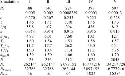
We perform a series of five different simulations, with Taylor microscale Reynolds numbers $R_{{\it\lambda}}\equiv 2k\sqrt{5/(3{\it\nu}{\it\epsilon})}$ ranging from 88 to 597, where $k$ denotes the turbulent kinetic energy and ${\it\epsilon}$ the turbulent energy dissipation rate. Details of the simulations are given in table 1. The simulations are parameterized to have similar large scales, but different dissipation (small) scales. 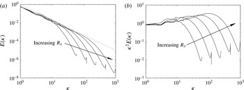The small-scale resolution for the simulations was held constant, with ${\it\kappa}_{\mathit{max}}{\it\eta}\approx 1.6{-}1.7$ , where ${\it\kappa}_{\mathit{max}}\equiv \sqrt{2}N/3$ is the maximum resolved wavenumber and ${\it\eta}\equiv ({\it\nu}^{3}/{\it\epsilon})^{1/4}$ is the Kolmogorov length scale. Dealiasing is performed using a combination of spherical truncation and phase shifting. Time-averaged energy and dissipation spectra for all five simulations are shown in figure 1. A clear $-5/3$ spectral slope is evident for the three highest Reynolds-number cases ( $R_{{\it\lambda}}\geqslant 224$ ), indicating the presence of a well-defined inertial subrange. The simulations are performed in parallel on $N_{\mathit{proc}}$ processors, and the P3DFFT library (Pekurovsky Reference Pekurovsky2012) is used for efficient parallel computation of three-dimensional fast Fourier transforms.

Figure 1.

(a) Energy and (b) dissipation spectra for the different simulations described in table 1. The diagonal dotted line in (a) has a slope of $-5/3$ , the expected spectral scaling in the inertial subrange. All values are in arbitrary units.

2.2 Particle phase

We simulate the motion of small ( $d/{\it\eta}\ll 1$ , where $d$ is the particle diameter), heavy ( ${\it\rho}_{p}/{\it\rho}_{f}\gg 1$ , where ${\it\rho}_{p}$ is the particle density), spherical particles. Eighteen different particle classes are simulated with Stokes numbers $St$ ranging from 0 to 30. $St\equiv {\it\tau}_{p}/{\it\tau}_{{\it\eta}}$ is a non-dimensional measure of a particle’s inertia, comparing the response time of the particle ${\it\tau}_{p}\equiv {\it\rho}_{p}d^{2}/(18{\it\rho}_{f}{\it\nu})$ to the Kolmogorov time scale ${\it\tau}_{{\it\eta}}\equiv ({\it\nu}/{\it\epsilon})^{1/2}$ .

We assume that the particles are subjected to only linear drag forces, which is a reasonable approximation when the particle Reynolds number $Re_{p}\equiv |\boldsymbol{u}(\boldsymbol{x}^{p}(t),t)-\boldsymbol{v}^{p}(t)|/{\it\nu}<0.5$ (Elghobashi & Truesdell Reference Elghobashi and Truesdell1992). Here, $\boldsymbol{u}(\boldsymbol{x}^{p}(t),t)$ denotes the undisturbed fluid velocity at the particle position $\boldsymbol{x}^{p}(t)$ and $\boldsymbol{v}^{p}(t)$ denotes the velocity of the particle. (Throughout this study, we use the superscript $p$ on $\boldsymbol{x}$ , $\boldsymbol{u}$ , and $\boldsymbol{v}$ to denote time-dependent Lagrangian variables defined along particle trajectories. Phase-space positions and velocities are denoted without the superscript $p$ .) Though particles with large $St$ experience non-negligible nonlinear drag forces (e.g. Wang & Maxey Reference Wang and Maxey1993), the use of a linear drag model for large- $St$ particles provides a useful first approximation and facilitates comparison between several theoretical models that make the same assumption (e.g. Chun et al. Reference Chun, Koch, Rani, Ahluwalia and Collins2005; Zaichik & Alipchenkov Reference Zaichik and Alipchenkov2009; Gustavsson & Mehlig Reference Gustavsson and Mehlig2011). We have also neglected the history force in this study. In an earlier work, Elghobashi & Truesdell (Reference Elghobashi and Truesdell1992) showed that the Basset history force is orders of magnitude smaller than the Stokes drag force when ${\it\rho}_{p}/{\it\rho}_{f}\gg 1$ (here our primary focus is on water droplets in air, where ${\it\rho}_{p}/{\it\rho}_{f}\sim 1000$ ). On this basis, most DNS of inertial particles in turbulence neglect this term, which involves an integral and is very expensive to compute. However, Daitche (Reference Daitche2015) showed that the Basset history term can slightly reduce particle clustering and collision rates for higher values of $St$ , and thus while we expect that our particle statistics generally have the correct leading-order behaviour, future studies are needed to systematically assess higher-order corrections to these statistics that result from the inclusion of the history force. The present study also neglects the influence of gravity. Part 2 of this study (Ireland et al. Reference Ireland, Bragg and Collins2016) will address the combined effects of gravity and turbulence on particle motion. Finally, since a primary motivation is to understand droplet dynamics in atmospheric clouds, where the particle mass and volume loadings are low (Shaw Reference Shaw2003), we assume that the particle loadings are sufficiently dilute such that interparticle interactions and two-way coupling between the phases are negligible (Elghobashi & Truesdell Reference Elghobashi and Truesdell1993; Sundaram & Collins Reference Sundaram and Collins1999).

Under these assumptions, each inertial particle obeys a simplified Maxey–Riley equation (Maxey & Riley Reference Maxey and Riley1983),

and each fluid (i.e. inertialess) particle is tracked by solving

To compute $\boldsymbol{u}^{p}(t)=\boldsymbol{u}(\boldsymbol{x}^{p}(t),t)$ , we need to interpolate from the Eulerian grid to the particle location. While other studies (e.g. see Bec et al. Reference Bec, Biferale, Cencini, Lanotte and Toschi2010a ; Durham et al. Reference Durham, Climent, Barry, Lillo, Boffetta, Cencini and Stocker2013) have done so using trilinear interpolation, Ireland et al. (Reference Ireland, Vaithianathan, Sukheswalla, Ray and Collins2013) showed that such an approach can lead to errors in the interpolated velocity that are orders of magnitude above the local time-stepping error. In addition, van Hinsberg et al. (Reference van Hinsberg, ten Thije Bookkkamp, Toschi and Clercx2013) demonstrated that trilinear interpolation, which possesses only $C^{0}$ continuity, leads to artificial high-frequency oscillations in the computed particle accelerations. Ray & Collins (Reference Ray and Collins2013) noted that the relative motion of particles at small separations will depend strongly on the interpolation scheme. Since a main focus of this paper is particle motion near contact and its influence on particle collisions, it is crucial to calculate $\boldsymbol{u}(\boldsymbol{x}^{p}(t),t)$ as accurately as possible. To that end, we use an eight-point B-spline interpolation scheme (with $C^{6}$ continuity) based on the algorithm in van Hinsberg et al. (Reference van Hinsberg, Thije Boonkkamp, Toschi and Clercx2012).

The particles were initially placed in the flow with a uniform distribution and velocities $\boldsymbol{v}^{p}$ equal to the underlying fluid velocity $\boldsymbol{u}^{p}$ . We began computing particle statistics once the particle distributions and velocities became statistically stationary, usually approximately 5 large eddy turnover times $T_{L}\equiv \ell /u^{\prime }$ (where $\ell$ is the integral length scale and $u^{\prime }\equiv \sqrt{2k/3}$ ) after the particles were introduced into the flow. Particle statistics were calculated at a frequency of 2–3 times per $T_{L}$ and were time averaged over the duration of the run  $T$ .

For a subset $N_{\mathit{tracked}}$ of the total number of particles in each class $N_{p}$ , we stored particle positions, velocities and velocity gradients every $0.1{\it\tau}_{{\it\eta}}$ for a duration of approximately $100{\it\tau}_{{\it\eta}}$ . These data are used to compute Lagrangian correlations, accelerations and time scales of the particles.

3.1 Velocity gradient statistics

We consider the gradients of the underlying fluid velocity at the particle locations, $\unicode[STIX]{x1D63C}(\boldsymbol{x}^{p}(t),t)\equiv \boldsymbol{{\rm\nabla}}\boldsymbol{u}(\boldsymbol{x}^{p}(t),t)$ . These statistics provide us with information about the small-scale velocity field experienced by the particles. (Refer to Meneveau (Reference Meneveau2011) for a recent review on this subject.) In particular, to understand the interaction of particles with specific topological features of the turbulence, we decompose $\unicode[STIX]{x1D63C}(\boldsymbol{x}^{p}(t),t)$ into a symmetric strain rate tensor $\unicode[STIX]{x1D64E}(\boldsymbol{x}^{p}(t),t)\equiv [\unicode[STIX]{x1D63C}(\boldsymbol{x}^{p}(t),t)+\unicode[STIX]{x1D63C}^{\text{T}}(\boldsymbol{x}^{p}(t),t)]/2$ and an antisymmetric rotation rate tensor $\unicode[STIX]{x1D64D}(\boldsymbol{x}^{p}(t),t)\equiv [\unicode[STIX]{x1D63C}(\boldsymbol{x}^{p}(t),t)-\unicode[STIX]{x1D63C}^{\text{T}}(\boldsymbol{x}^{p}(t),t)]/2$ .

Figure 2.

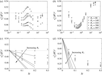
Data for $\langle \unicode[STIX]{x1D61A}^{2}\rangle ^{p}$ (a,c) and $\langle \unicode[STIX]{x1D619}^{2}\rangle ^{p}$ (b,d) sampled at inertial particle positions as function of $St$ for different values of $R_{{\it\lambda}}$ . The data are shown at low $St$ in (c,d) to highlight the effect of preferential sampling in this regime. The solid lines in (c,d) are the predictions from (3.3) for $St\ll 1$ . DNS data are shown with symbols.

Due to their inertia, heavy particles are ejected out of regions of high rotation rate and accumulate in regions of high strain rate (e.g. Maxey Reference Maxey1987; Squires & Eaton Reference Squires and Eaton1991; Eaton & Fessler Reference Eaton and Fessler1994), and this is associated with a ‘preferential sampling’ of $\unicode[STIX]{x1D63C}(\boldsymbol{x},t)$ . For particles with low inertia ( $St\ll 1$ ), preferential sampling is the dominant mechanism affecting the particle motion (e.g. see Chun et al. Reference Chun, Koch, Rani, Ahluwalia and Collins2005). As the particle inertia increases, the particle motion becomes increasingly decoupled from the local fluid turbulence, and the effect of the preferential sampling on the particle dynamics decreases. At the other limit ( $St\gg 1$ ), preferential sampling vanishes and the particles have a damped response to the underlying flow which leads them to sample the turbulence more uniformly (e.g. see Bec et al. Reference Bec, Biferale, Boffetta, Celani, Cencini, Lanotte, Musacchio and Toschi2006a ).

We first consider the average of the second invariants of the strain rate and rotation rate tensors evaluated at the inertial particle positions

and

By definition, for fully mixed fluid particles ( $St=0$ ) in homogeneous turbulence, ${\it\tau}_{{\it\eta}}^{2}\langle \unicode[STIX]{x1D61A}^{2}\rangle ^{p}={\it\tau}_{{\it\eta}}^{2}\langle \unicode[STIX]{x1D619}^{2}\rangle ^{p}=0.5$ .

Since small- $St$ particles are centrifuged out of regions of high rotation, we expect that ${\it\tau}_{{\it\eta}}^{2}\langle \unicode[STIX]{x1D619}^{2}\rangle ^{p}$ will decrease with increasing $St$ ; their accumulation in high strain regions would also lead to the expectation that ${\it\tau}_{{\it\eta}}^{2}\langle \unicode[STIX]{x1D61A}^{2}\rangle ^{p}$ will increase with increasing $St$ . In figure 2 we see that while ${\it\tau}_{{\it\eta}}^{2}\langle \unicode[STIX]{x1D619}^{2}\rangle ^{p}$ is more strongly affected by changes in $R_{{\it\lambda}}$ than is ${\it\tau}_{{\it\eta}}^{2}\langle \unicode[STIX]{x1D61A}^{2}\rangle ^{p}$ , both quantities decrease with increasing $St$ (for $St\ll 1$ ). This surprising result is consistent with other DNS (Collins & Keswani Reference Collins and Keswani2004; Chun et al. Reference Chun, Koch, Rani, Ahluwalia and Collins2005; Salazar & Collins Reference Salazar and Collins2012a ). Our data also show that both ${\it\tau}_{{\it\eta}}^{2}\langle \unicode[STIX]{x1D61A}^{2}\rangle ^{p}$ and ${\it\tau}_{{\it\eta}}^{2}\langle \unicode[STIX]{x1D619}^{2}\rangle ^{p}$ decrease with increasing $R_{{\it\lambda}}$ for $St\ll 1$ , in agreement with Collins & Keswani (Reference Collins and Keswani2004).

We use the formulation given in Chun et al. (Reference Chun, Koch, Rani, Ahluwalia and Collins2005) (and rederived in Salazar & Collins (Reference Salazar and Collins2012a )) to model the effect of preferential sampling on ${\it\tau}_{{\it\eta}}^{2}\langle \unicode[STIX]{x1D61A}^{2}\rangle ^{p}$ and ${\it\tau}_{{\it\eta}}^{2}\langle \unicode[STIX]{x1D619}^{2}\rangle ^{p}$ in limit of $St\ll 1$ . Chun et al. (Reference Chun, Koch, Rani, Ahluwalia and Collins2005) and Salazar & Collins (Reference Salazar and Collins2012a ) showed that for an arbitrary quantity ${\it\phi}$ , the average value of ${\it\phi}$ sampled along a particle trajectory $\langle {\it\phi}\rangle ^{p}$ can be reconstructed entirely from fluid particle statistics using the relation,

Here, ${\it\sigma}_{Y}^{p}$ denotes the standard deviation of a variable $Y$ along a fluid particle trajectory, ${\it\rho}_{YZ}^{p}$ is the correlation coefficient between $Y$ and $Z$ ,

and $T_{YZ}^{p}$ is the Lagrangian correlation time,

The predictions from (3.3) for small $St$ are shown by the solid lines in figure 2(c,d). The data at the highest Reynolds numbers provide the first test of the predictions from Chun et al. (Reference Chun, Koch, Rani, Ahluwalia and Collins2005) for flows with a well-defined inertial range. In the limit of small $St$ , (3.3) is able to capture the decrease in both ${\it\tau}_{{\it\eta}}^{2}\langle \unicode[STIX]{x1D61A}^{2}\rangle ^{p}$ and ${\it\tau}_{{\it\eta}}^{2}\langle \unicode[STIX]{x1D619}^{2}\rangle ^{p}$ with increasing $St$ , and also the decrease in these quantities with increasing $R_{{\it\lambda}}$ . It is uncertain whether the quantitative differences between the DNS data and the model are due to shortcomings of the model or the fact that the smallest inertial particles ( $St=0.05$ ) are too large for the model (which assumes $St\ll 1$ ) to hold.

An important implication of these results is that the degree of preferential sampling (and thus indirectly, the amount of clustering) of inertial particles can be predicted using experimental or DNS data measured along fluid particle trajectories. Such data are generally more widely available at even higher Reynolds numbers than those simulated here and could provide an indication of the trends in preferential sampling at such conditions.

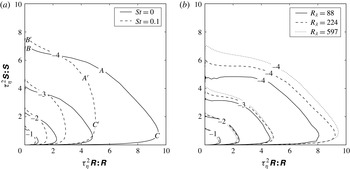
Despite the success of the model of Chun et al. (Reference Chun, Koch, Rani, Ahluwalia and Collins2005) in reproducing the trends in the DNS, the physical explanation for the changes in the mean strain and rotation rates remains unclear. In figure 3(a), we plot joint probability density functions (PDFs) of the strain and rotation rates sampled by both $St=0$ and $St=0.1$ particles to better understand the specific topological features of the regions of the flow contributing to these changes. Following the designations given in Soria et al. (Reference Soria, Sondergaard, Cantwell, Chong and Perry1994), we refer to regions with high strain and high rotation (indicated by ‘ $A$ ’ in figure 3 a) as ‘vortex sheets’, regions of low rotation and high strain (indicated by ‘ $B$ ’) as ‘irrotational dissipation’ areas, and regions of high rotation and low strain (indicated by ‘ $C$ ’) as ‘vortex tubes.’

Figure 3.

(a) Joint PDFs of ${\it\tau}_{{\it\eta}}^{2}\unicode[STIX]{x1D64E}\boldsymbol{ : }\unicode[STIX]{x1D64E}$ and ${\it\tau}_{{\it\eta}}^{2}\unicode[STIX]{x1D64D}\boldsymbol{ : }\unicode[STIX]{x1D64D}$ for $R_{{\it\lambda}}=597$ for $St=0$ and $St=0.1$ particles. Certain regions of the flow are labelled to aid in the discussion of the trends. (b) Joint PDFs of ${\it\tau}_{{\it\eta}}^{2}\unicode[STIX]{x1D64E}\boldsymbol{ : }\unicode[STIX]{x1D64E}$ and ${\it\tau}_{{\it\eta}}^{2}\unicode[STIX]{x1D64D}\boldsymbol{ : }\unicode[STIX]{x1D64D}$ for different $R_{{\it\lambda}}$ for $St=0$ particles. In both plots, the exponents of the decade are indicated on the contour lines.

We see that the inertial particle PDFs differ from those of fluid particles in three primary ways. First, inertial particles are less likely to occupy vortex sheets ( $A$ ) and are more likely to occupy regions of moderate rotation and moderate strain ( $A^{\prime }$ ). This undersampling of vortex sheets has only recently been discussed in the literature (Salazar & Collins Reference Salazar and Collins2012a ). Second, inertial particles are more likely to be found in irrotational dissipation regions, where they preferentially sample regions of higher strain (e.g. compare $B$ and $B^{\prime }$ ). Third, inertial particles are less likely to be found in vortex tubes ( $C$ ) and more likely to be found in regions of lower rotation and higher strain ( $C^{\prime }$ ). Evidently, this first trend is primarily responsible for the decrease in ${\it\tau}_{{\it\eta}}^{2}\langle \unicode[STIX]{x1D61A}^{2}\rangle ^{p}$ at small $St$ , as suggested in Salazar & Collins (Reference Salazar and Collins2012a ), and the first and third trends both contribute to the decrease in ${\it\tau}_{{\it\eta}}^{2}\langle \unicode[STIX]{x1D619}^{2}\rangle ^{p}$ . We will revisit these three trends in relation to the particle kinetic energies (§ 3.2) and the particle accelerations (§ 3.3).

Figure 3(b) shows the PDF map for fluid particles at three values of the Reynolds number. Notice that as $R_{{\it\lambda}}$ increases, the probability of encountering a vortex sheet (overlapping high strain and high rotation) increases. This finding is consistent with the results of Yeung et al. (Reference Yeung, Donzis and Sreenivasan2012), who observed that high strain and rotation events increasingly overlap in isotropic turbulence as the Reynolds number increases. It is thus likely that with increasing Reynolds number, rotation and strain events become increasingly intense and the resulting vortex sheets become increasingly efficient at expelling particles, causing both ${\it\tau}_{{\it\eta}}^{2}\langle \unicode[STIX]{x1D61A}^{2}\rangle ^{p}$ and ${\it\tau}_{{\it\eta}}^{2}\langle \unicode[STIX]{x1D619}^{2}\rangle ^{p}$ to decrease (cf. figure 2).

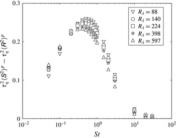
Maxey (Reference Maxey1987) noted that at low $St$ , the compressibility of the particle field (and hence the degree of particle clustering) is directly related to the difference between the rates of strain and rotation sampled by the particles, ${\it\tau}_{{\it\eta}}^{2}\langle \unicode[STIX]{x1D61A}^{2}\rangle ^{p}-{\it\tau}_{{\it\eta}}^{2}\langle \unicode[STIX]{x1D619}^{2}\rangle ^{p}$ . From figure 4, we see that at low $St$ , ${\it\tau}_{{\it\eta}}^{2}\langle \unicode[STIX]{x1D61A}^{2}\rangle ^{p}-{\it\tau}_{{\it\eta}}^{2}\langle \unicode[STIX]{x1D619}^{2}\rangle ^{p}$ increases with increasing $R_{{\it\lambda}}$ , suggesting that the degree of clustering may also increase here. We will test this hypothesis in § 4.2 when we directly measure particle clustering at different values of $St$ and $R_{{\it\lambda}}$ .

Figure 4.

The difference between the mean rates of strain and rotation sampled by the particles as a function of $St$ for different values of $R_{{\it\lambda}}$ .

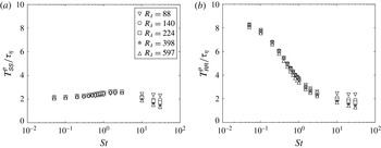
We finally consider the Lagrangian strain and rotation time scales, which will be useful for understanding the trends in particle clustering in § 4.2. Since the fluid and particle phases are isotropic, we will have nine statistically equivalent strain time scales: $T_{\unicode[STIX]{x1D61A}_{11}\unicode[STIX]{x1D61A}_{11}}^{p}$ , $T_{\unicode[STIX]{x1D61A}_{11}\unicode[STIX]{x1D61A}_{22}}^{p}$ , $T_{\unicode[STIX]{x1D61A}_{11}\unicode[STIX]{x1D61A}_{33}}^{p}$ , $T_{\unicode[STIX]{x1D61A}_{12}\unicode[STIX]{x1D61A}_{12}}^{p}$ , $T_{\unicode[STIX]{x1D61A}_{13}\unicode[STIX]{x1D61A}_{13}}^{p}$ , $T_{\unicode[STIX]{x1D61A}_{22}\unicode[STIX]{x1D61A}_{22}}^{p}$ , $T_{\unicode[STIX]{x1D61A}_{22}\unicode[STIX]{x1D61A}_{33}}^{p}$ , $T_{\unicode[STIX]{x1D61A}_{23}\unicode[STIX]{x1D61A}_{23}}^{p}$ and $T_{\unicode[STIX]{x1D61A}_{33}\unicode[STIX]{x1D61A}_{33}}^{p}$ . We take the strain time scale $T_{\unicode[STIX]{x1D61A}\unicode[STIX]{x1D61A}}^{p}$ to be the average of these nine components. We similarly take the rotation time scale $T_{\unicode[STIX]{x1D619}\unicode[STIX]{x1D619}}^{p}$ to be the average of three statistically equivalent components: $T_{\unicode[STIX]{x1D619}_{12}\unicode[STIX]{x1D619}_{12}}^{p}$ , $T_{\unicode[STIX]{x1D619}_{13}\unicode[STIX]{x1D619}_{13}}^{p}$ and $T_{\unicode[STIX]{x1D619}_{23}\unicode[STIX]{x1D619}_{23}}^{p}$ .

Figure 5.

Lagrangian time scales of a single component of the strain rate (a) and rotation rate (b) tensors, plotted as a function of $St$ for different values of $R_{{\it\lambda}}$ .

We see that $T_{\unicode[STIX]{x1D61A}\unicode[STIX]{x1D61A}}^{p}/{\it\tau}_{{\it\eta}}$ is independent of $R_{{\it\lambda}}$ for $St<10$ , and decreases weakly with increasing $R_{{\it\lambda}}$ for $St\geqslant 10$ . On the other hand, $T_{\unicode[STIX]{x1D619}\unicode[STIX]{x1D619}}^{p}/{\it\tau}_{{\it\eta}}$ tends to decrease with increasing $R_{{\it\lambda}}$ for all values of $St$ , and this decrease becomes more pronounced as $St$ increases. We also see that $T_{\unicode[STIX]{x1D619}\unicode[STIX]{x1D619}}^{p}$ is much more sensitive to changes in $St$ than $T_{\unicode[STIX]{x1D61A}\unicode[STIX]{x1D61A}}^{p}$ , suggesting that the dominant effect of inertia is to cause particles to spend less time in strongly rotating regions. As a result, the particles will generally have less time to respond to fluctuations in the rotation rate, causing $\langle \unicode[STIX]{x1D619}^{2}\rangle ^{p}$ to be strongly reduced with increasing $St$ , as was seen above.

3.2 Particle kinetic energy

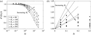
We now move from small-scale velocity statistics to large-scale velocity statistics. Figure 6 shows the average particle kinetic energy $k^{p}(St)\equiv \langle \boldsymbol{v}^{p}(t)\boldsymbol{\cdot }\boldsymbol{v}^{p}(t)\rangle /2$ (normalized by the average fluid kinetic energy $k$ ) for different values of $R_{{\it\lambda}}$ .

Figure 6.

(a) The ratio between the average particle kinetic energy $k^{p}(St)$ and the average fluid kinetic energy $k$ for different values of $R_{{\it\lambda}}$ . DNS data are shown with symbols and the predictions of the filtering model in (3.6) are shown with solid lines. (b) The ratio between $k^{p}(St)$ and $k$ (open symbols) and the ratio between the average fluid kinetic energy at the particle locations $k^{fp}(St)$ and $k$ (filled symbols), shown at low $St$ to highlight the effects of preferential sampling. Also shown is the prediction from the preferential sampling model given in (3.3) (solid lines).

We first consider the effect of inertial filtering on this statistic and then examine the effect of preferential sampling. It is well known that filtering leads to a reduction in the particle turbulent kinetic energy for large values of $St$ . This reduction is the strongest for the lowest Reynolds numbers and the weakest for the highest Reynolds numbers, as seen in figure 6(a). These trends are captured by the model in Abrahamson (Reference Abrahamson1975), which assumes an exponential decorrelation of the Lagrangian fluid velocity. Under this assumption, the ratio between the particle and fluid kinetic energies can be expressed as

where ${\it\tau}_{\ell }$ is the Lagrangian correlation time of the fluid, which we approximate using the relation given in Zaichik, Simonin & Alipchenkov (Reference Zaichik, Simonin and Alipchenkov2003). The model predictions of $k^{p}(St)/k$ are included in figure 6(a) and are in good agreement with the DNS at large $St$ , where filtering is dominant. The trends with $R_{{\it\lambda}}$ are also reproduced well.

We thus have the following physical explanation of inertial filtering on the particle kinetic energies: for low-Reynolds-number flows, the response time of the largest particles exceeds the time scales of many large-scale flow features. The result is a filtered response to the large-scale turbulence and an overall reduction in the particle kinetic energy. As the Reynolds number is increased (and the particle response time is fixed with respect to the small-scale turbulence), more flow features are present with time scales that exceed the particle response time, and hence the effect of inertial filtering is diminished with increasing $R_{{\it\lambda}}$ , as predicted by (3.6).

To highlight the effect of preferential sampling on the particle kinetic energy, figure 6(b) shows both the average particle kinetic energy $k^{p}(St)$ and the average kinetic energy of the fluid sampled along an inertial particle trajectory, $k^{fp}(St)\equiv \langle \boldsymbol{u}(\boldsymbol{x}^{p}(t),t)\boldsymbol{\cdot }\boldsymbol{u}(\boldsymbol{x}^{p}(t),t)\rangle /2$ . As is evident in figure 6(b), the particle kinetic energy exceeds $k$ for low values of $St$ . By comparing $k^{p}$ to $k^{fp}$ , we see that the increased kinetic energy of the smallest particles is due almost entirely to preferential sampling of the flow field. While Salazar & Collins (Reference Salazar and Collins2012b ) were the first to show an increase in $k^{p}(St)/k$ for low $St$ (which they attributed to preferential sampling), this trend is also suggested by the early study of Squires & Eaton (Reference Squires and Eaton1991), in which the authors observed that small inertial particles preferentially sample certain high kinetic energy regions they referred to as ‘streaming zones.’ Figure 6(b) also shows that at small values of $St$ , $k^{p}(St)/k$ decreases with increasing Reynolds number.

The solid lines in figure 6(b) show the predictions of the particle kinetic energy from (3.3). In the limit of small $St$ , the model of Chun et al. (Reference Chun, Koch, Rani, Ahluwalia and Collins2005) is able to capture qualitatively both the increase in $k^{p}(St)/k$ with increasing $St$ and the decrease in $k^{p}(St)/k$ with increasing  $R_{{\it\lambda}}$ .

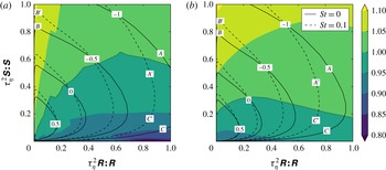
To further elucidate the physical mechanisms leading to these trends, we plot the mean kinetic energy of the fluid conditioned on $\unicode[STIX]{x1D61A}^{2}$ and $\unicode[STIX]{x1D619}^{2}$ , $k_{\unicode[STIX]{x1D61A}^{2},\unicode[STIX]{x1D619}^{2}}$ , in figure 7. Isocontours of the concentrations of $St=0$ and $St=0.1$ particles are shown for comparison. (To reduce the statistical noise in the conditional averages and to focus on the regions where most particles are present, we consider a narrower range of $\unicode[STIX]{x1D61A}^{2}$ and $\unicode[STIX]{x1D619}^{2}$ than in figure 3. The trends discussed below, however, are still evident when we consider the same range of $\unicode[STIX]{x1D61A}^{2}$ and $\unicode[STIX]{x1D619}^{2}$ as before.) While the data contain considerable statistical noise, we can draw a few conclusions about the qualitative trends.

Figure 7.

Filled contours of the fluid kinetic energy conditioned on $\unicode[STIX]{x1D61A}^{2}$ and $\unicode[STIX]{x1D619}^{2}$ , $k_{\unicode[STIX]{x1D61A}^{2},\unicode[STIX]{x1D619}^{2}}$ , normalized by the unconditioned mean fluid kinetic energy $k$ at (a) the lowest Reynolds number and (b) the highest Reynolds number. The dotted contour lines indicate $k_{\unicode[STIX]{x1D61A}^{2},\unicode[STIX]{x1D619}^{2}}/k=1$ . Isocontours of particle concentration for $St=0$ and $St=0.1$ particles are included for reference, with the exponents of the decade indicated on the contour lines. Certain regions of the flow are labelled to aid in the discussion of the trends.

From figure 7(a), we see that the change in kinetic energy at $R_{{\it\lambda}}=88$ can be divided into the three mechanisms discussed in § 3.1. First, particles are less likely to sample vortex sheets ( $A$ ) and are more likely to sample moderate rotation and moderate strain regions ( $A^{\prime }$ ). This behaviour generally tends to decrease the particle kinetic energy. Second, as $St$ increases, particles preferentially sample regions of higher strain ( $B^{\prime }$ ), which are characterized by higher kinetic energy. Third, some inertial particles are less likely to occupy vortex tubes ( $C$ ), which are characterized by lower kinetic energies, and are more likely to occupy lower rotation and higher strain regions ( $C^{\prime }$ ), which have higher kinetic energies. The observed increase in $k^{p}(St)/k$ must therefore be due to the second and third trends.

At high Reynolds numbers, however, overlapping high rotation/high strain regions of the flow occur with a higher probability (as shown in § 3.1), and inertial particles tend to avoid these regions. The first trend (which tends to decrease the kinetic energy) therefore plays a larger role. Also, at $R_{{\it\lambda}}=597$ , high rotation and low strain regions (e.g. see region $C$ in figure 7 b) are no longer associated with very low kinetic energies, causing the third trend to be less effective at increasing the particle kinetic energy. The overall result is a decrease in $k^{p}(St)/k$ with increasing Reynolds number at small values of  $St$ .

3.3 Particle accelerations

In this section, we analyse fluid and inertial particle accelerations $\boldsymbol{a}^{p}(t)\equiv \text{d}\boldsymbol{v}^{p}(t)/\text{d}t$ . Fluid particle accelerations are known to be strongly intermittent (e.g. see Voth et al. Reference Voth, La Porta, Crawford, Alexander and Bodenschatz2002; Ishihara et al. Reference Ishihara, Kaneda, Yokokawa, Itakura and Uno2007), with the probability of intense acceleration events increasing with the Reynolds number. Before accounting for inertial effects, we consider the effect of $R_{{\it\lambda}}$ on the acceleration variance $\langle a^{2}\rangle ^{p}\equiv \langle \boldsymbol{a}^{p}(t)\boldsymbol{\cdot }\boldsymbol{a}^{p}(t)\rangle /3$ of Lagrangian fluid particles in figure 8(a). To facilitate comparison between the different Reynolds numbers, we have normalized $\langle a^{2}\rangle ^{p}$ by the Kolmogorov acceleration variance $a_{{\it\eta}}^{2}\equiv \sqrt{{\it\epsilon}^{3}/{\it\nu}}$ . 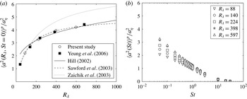The DNS data from Yeung et al. (Reference Yeung, Pope, Lamorgese and Donzis2006) and the theoretical predictions of Hill (Reference Hill2002), Sawford et al. (Reference Sawford, Yeung, Borgas, La Porta, Crawford and Bodenschatz2003) and Zaichik et al. (Reference Zaichik, Simonin and Alipchenkov2003) are shown for comparison. We see that our DNS data agrees well with Yeung et al. (Reference Yeung, Pope, Lamorgese and Donzis2006), and that the model of Sawford et al. (Reference Sawford, Yeung, Borgas, La Porta, Crawford and Bodenschatz2003) best reproduces the trends in the DNS. Hill (Reference Hill2002) breaks down at low $R_{{\it\lambda}}$ while Zaichik et al. (Reference Zaichik, Simonin and Alipchenkov2003) fails at high $R_{{\it\lambda}}$ .

Figure 8.

(a) The acceleration variance of Lagrangian fluid particles as a function of $R_{{\it\lambda}}$ . The results from the present study (open circles) are compared to DNS data from Yeung et al. (Reference Yeung, Pope, Lamorgese and Donzis2006) (filled squares) and several theoretical predictions (lines). (b) The acceleration variance of inertial particles as a function of $St$ for different values of $R_{{\it\lambda}}$ .

We turn our attention to inertial particle accelerations in figure 8(b). The observed trend for inertial particles is analogous to that for fluid particles: at each value of $St$ considered, the particle acceleration variance (normalized by Kolmogorov units) monotonically increases with $R_{{\it\lambda}}$ (cf. Bec et al. Reference Bec, Biferale, Boffetta, Celani, Cencini, Lanotte, Musacchio and Toschi2006a ). As $St$ increases, the acceleration variance decreases, presumably as a result of both preferential sampling of the flow field and inertial filtering.

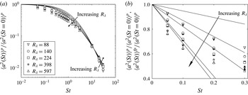
We now seek to understand and model how inertia changes the accelerations of particles through the filtering and preferential sampling effects. To do so, we rescale the inertial particle acceleration variance by that of fluid particles and plot the results in figure 9. In figure 9(a), we compare the rescaled acceleration variance to the model of Zaichik & Alipchenkov (Reference Zaichik and Alipchenkov2008), which only accounts for inertial filtering of the underlying flow. The model of Zaichik & Alipchenkov (Reference Zaichik and Alipchenkov2008) is able to capture all the qualitative trends in $R_{{\it\lambda}}$ and $St$ , and the model predictions provide remarkably good quantitative agreement with the DNS at the largest values of $St$ , where filtering is the dominant mechanism. At lower values of $St$ , the rescaled particle acceleration variance decreases with increasing $R_{{\it\lambda}}$ . In this case, as $R_{{\it\lambda}}$ increases, the underlying flow is subjected to increasingly intermittent acceleration events, and the inertial particles filter a larger fraction of these events. At the largest values of $St$ , most intermittent accelerations are filtered, and a particle’s acceleration variance is determined by its interaction with the largest turbulence scales. Since the range of available large scales increases with $R_{{\it\lambda}}$ , the rescaled particle acceleration variance increases with $R_{{\it\lambda}}$ for the largest values of $St$ .

Figure 9.

(a) Inertial particle acceleration variances scaled by the fluid particle acceleration variance (open symbols). The solid lines and arrows indicate the predictions from the filtering model of Zaichik & Alipchenkov (Reference Zaichik and Alipchenkov2008). (b) The variance of the inertial particle accelerations (open symbols) and the fluid accelerations sampled at the inertial particle positions (filled symbols), shown at low $St$ to highlight the effect of preferential sampling. The solid lines indicate the predictions from the preferential sampling model given in (3.3).

We now consider the effect of preferential sampling on the acceleration variances. To do so, we also compute the acceleration of the fluid sampled by inertial particles, defined as

The variance of $\boldsymbol{a}^{fp}$ is denoted as $\langle a^{2}\rangle ^{fp}\equiv \langle \boldsymbol{a}^{fp}(t)\boldsymbol{\cdot }\boldsymbol{a}^{fp}(t)\rangle /3$ . In figure 9(b), we plot both $\langle a^{2}\rangle ^{p}$ and $\langle a^{2}\rangle ^{fp}$ (scaled by the acceleration variance of $St=0$ particles). As expected, for $St\ll 1$ , where preferential sampling is the dominant mechanism, inertial particle accelerations are almost equivalent to the accelerations of the underlying flow sampled at inertial particle positions. The model of Chun et al. (Reference Chun, Koch, Rani, Ahluwalia and Collins2005) (equation (3.3) above) is able to reproduce all the qualitative trends correctly in the limit of small $St$ . The scaled variances decrease with increasing $R_{{\it\lambda}}$ , and we expect that this trend is due to the fact that high vorticity regions are associated with high accelerations (Biferale et al. Reference Biferale, Boffetta, Celani, Lanotte and Toschi2005) and become increasingly efficient at ejecting particles (refer to § 3.1).

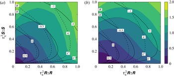
We test this expectation in figure 10 by plotting the acceleration variance for fluid particles conditioned on $\unicode[STIX]{x1D61A}^{2}$ and $\unicode[STIX]{x1D619}^{2}$ , $\langle a^{2}\rangle _{\unicode[STIX]{x1D61A}^{2},\unicode[STIX]{x1D619}^{2}}^{p}$ , and normalized by the unconditioned variance $\langle a^{2}\rangle ^{p}$ . We see that inertial particles do indeed undersample high vorticity regions (both vortex sheets and vortex tubes) and preferentially sample lower vorticity regions (e.g. compare $A$ and $A^{\prime }$ and $C$ and $C^{\prime }$ ) and that these high vorticity regions are marked by very large accelerations. Though some inertial particles experience higher accelerations as they preferentially sample irrotational straining regions with higher strain rates (e.g. compare $B$ and $B^{\prime }$ ), this effect is relatively weak and the overall trend is a decrease in the particle accelerations with increasing inertia.

Figure 10.

Filled contours of the variance of the fluid particle accelerations conditioned on $\unicode[STIX]{x1D61A}^{2}$ and $\unicode[STIX]{x1D619}^{2}$ , $\langle a^{2}\rangle _{\unicode[STIX]{x1D61A}^{2},\unicode[STIX]{x1D619}^{2}}^{p}$ , normalized by the unconditioned fluid particle acceleration variance $\langle a^{2}\rangle ^{p}$ , at (a) $R_{{\it\lambda}}=88$ and (b) $R_{{\it\lambda}}=597$ . The dotted contour lines indicate $\langle a^{2}\rangle _{\unicode[STIX]{x1D61A}^{2},\unicode[STIX]{x1D619}^{2}}^{p}/\langle a^{2}\rangle ^{p}=1$ . Isocontours of particle concentration for $St=0$ and $St=0.1$ particles are included for reference, with the exponents of the decade indicated on the contour lines. Certain regions of the flow are labelled to aid in the discussion of the trends.

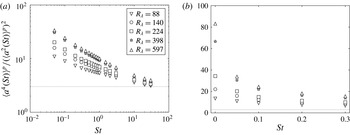
To investigate the intermittency of inertial particle accelerations, we plot the kurtosis of the particle accelerations, $\langle a^{4}\rangle ^{p}/(\langle a^{2}\rangle ^{p})^{2}$ , in figure 11, where $\langle a^{4}\rangle ^{p}\equiv \langle a_{1}^{p}(t)^{4}+a_{2}^{p}(t)^{4}+a_{3}^{p}(t)^{4}\rangle ^{p}/3$ . (Note that a Gaussian distribution has a kurtosis of 3, as indicated in figure 11 by a dotted line.) As expected, the particle accelerations are highly intermittent, with the degree of intermittency increasing with increasing $R_{{\it\lambda}}$ . We note that this trend in the kurtosis with $R_{{\it\lambda}}$ seems to be entirely due to the fluid flow intermittency. In fact, when we divide the acceleration kurtosis values of inertial particles by those of fluid particles (not shown), we observe the opposite trend with $R_{{\it\lambda}}$ , suggesting that inertial particles are affected less by intermittent events than fluid particles are. This is consistent with our explanations for trends in the particle acceleration variances given above, as well as with Bec et al. (Reference Bec, Biferale, Cencini, Lanotte and Toschi2006c ), who found that inertial particles undersample the most highly intermittent turbulent events in the fluid.

The kurtosis decreases very rapidly as $St$ increases. Figure 11(b) indicates that the kurtosis of very small particles ( $St=0.05$ ) at the highest value of $R_{{\it\lambda}}$ is over a factor of two smaller than that of fluid particles. The largest- $St$ particles have kurtosis values approaching those of a Gaussian distribution. These trends can be explained by the fact that both preferential sampling and inertial filtering decrease the probability of high-intensity acceleration events. Standardized moments of up to order $10$ (not shown) were also analysed and found to exhibit the same trends.

Figure 11.

Particle acceleration kurtosis as a function of $St$ for different values of $R_{{\it\lambda}}$ . The dotted line indicates a kurtosis of 3, the value for a Gaussian distribution. Values over the whole range of non-zero $St$ are shown in (a). (b) Shows only small- $St$ results on a linear plot to emphasize the rapid reduction in kurtosis as $St$ increases from 0.

We should note that the grid resolution study in Yeung et al. (Reference Yeung, Pope, Lamorgese and Donzis2006) suggests that the acceleration moments from our DNS may be underpredicted. Yeung et al. (Reference Yeung, Pope, Lamorgese and Donzis2006) showed that at $R_{{\it\lambda}}\approx 140$ , increasing the grid resolution $k_{\mathit{max}}{\it\eta}$ from 1.5 to 12 led to a 10 % increase in the fluid acceleration variance and a 30 % increase in the fluid acceleration kurtosis. It is unclear how these trends will change at higher $R_{{\it\lambda}}$ , but it suggests that the quantitative results reported here should be interpreted with caution. (The velocity gradients presented earlier are likely reliable, however, since Yeung et al. (Reference Yeung, Pope, Lamorgese and Donzis2006) found that such statistics are less dependent on the grid resolution.)

4.1 Particle relative velocities

We study particle relative velocities as a function of both $St$ and $R_{{\it\lambda}}$ . The relative velocities for inertial particles are defined by the relation

Here, $\boldsymbol{v}_{1}^{p}$ and $\boldsymbol{v}_{2}^{p}$ indicate the velocities of particles 1 and 2, respectively, which are separated from each other by a distance $r^{p}(t)=|\boldsymbol{r}^{p}(t)|$ . The subscripts $\Vert$ and $\bot$ indicate directions parallel (longitudinal) to the separation vector or perpendicular (transverse) to the separation vector, respectively, and $\boldsymbol{e}_{\Vert ,\bot }^{p}$ denotes the unit vector in the corresponding direction. (We use the method discussed in Pan & Padoan (Reference Pan and Padoan2013) to compute the transverse components. Pan & Padoan (Reference Pan and Padoan2013) set up a local coordinate system for each particle pair, and choose one unit vector of the coordinate system to align with the separation vector between the particles. They then apply two successive rotations to this unit vector to define two transverse unit vectors, which are used to compute two statistically equivalent transverse relative velocity components.)

We will also examine the velocity differences of the fluid at the particle locations, defined as

where $\boldsymbol{u}_{1}^{p}$ and $\boldsymbol{u}_{2}^{p}$ are the velocities of the fluid underlying particles 1 and 2, respectively. Note that for uniformly distributed fluid ( $St=0$ ) particles, the particle velocity statistics are equivalent to the underlying fluid velocity statistics.

Following the nomenclature in Bragg & Collins (Reference Bragg and Collins2014a ,Reference Bragg and Collins b ), we denote particle relative velocity moments of order $n$ as

for the components parallel to the separation vector, and as

for components perpendicular to the separation vector. In these expressions $\langle \cdot \rangle _{r}$ denotes an ensemble average conditioned on $r^{p}(t)=r$ .

For the purposes of computing the collision kernel (see § 4.3), we are also interested in the mean inward relative velocity parallel to the separation vector, defined as

where $p(w_{\Vert }|r)=\langle {\it\delta}(w_{\Vert }^{p}(t)-w_{\Vert })\rangle _{r}$ is the PDF for the longitudinal particle relative velocity conditioned on $r^{p}(t)=r$ .

Finally, in some cases we are also interested in moments of the fluid velocity differences. We use a superscript $fp$ to denote the moments of fluid velocity differences at the particle locations, and a superscript $f$ to denote the moments of fluid velocity differences at fixed points with separation $r$ . We therefore have

and

The components perpendicular to the separation vector are defined analogously.

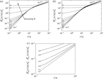
In figure 12, we plot the relative velocity variances $S_{2\Vert }^{p}$ and $S_{2\bot }^{p}$ versus $r/{\it\eta}$ at $R_{{\it\lambda}}=597$ . The mean inward relative velocity (not shown) has the same qualitative trends and will be considered later in this section. For the purposes of the following discussion, we define the dissipation range as the region over which the fluid velocity variances follow $r^{2}$ -scaling, which is seen to be $0\leqslant r/{\it\eta}\lesssim 10$ in figure 12, in agreement with Ishihara et al. (Reference Ishihara, Gotoh and Kaneda2009).

Figure 12.

The particle relative velocity variances parallel to the separation vector (a) and perpendicular to the separation vector (b), plotted as a function of the separation $r/{\it\eta}$ for $R_{{\it\lambda}}=597$ . The Stokes numbers are indicated by the line labels, and the $St=0$ curves are shown with dashed lines for clarity. The expected dissipation and inertial range scalings (based on Kolmogorov Reference Kolmogorov1941) are included for reference. In (c), we have included parallel and perpendicular relative velocities at small $St$ and small separations to highlight the behaviour in this regime. $S_{2\Vert }^{p}$ values are plotted with solid lines, and $S_{2\bot }^{p}$ values with dotted lines. The Stokes numbers are indicated by the line labels.

At small separations, the relative velocity variances parallel to the separation vector (figure 12 a) increase monotonically with $St$ and deviate from $r^{2}$ -scaling, while the relative velocity variances perpendicular to the separation vector decrease for $St\lesssim 0.1$ and then increase monotonically with $St$ for $St\gtrsim 0.1$ (figure 12 b). We expect that the trends at small separations and small $St$ are primarily due to preferential sampling of the underlying flow, which also dictates much of the single-particle dynamics for small $St$ (refer to § 3).

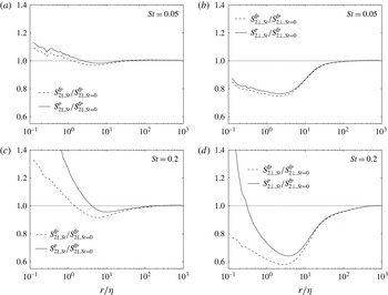
To test this expectation, we compare the particle relative velocity variances to those of the fluid sampled by the particles in figure 13. In all cases, the velocity variances are normalized by those of $St=0$ particles. At $St=0.05$ (figure 13 a,b), the effect of preferential sampling is dominant at all separations, as evidenced by the fact that $S_{2\Vert }^{fp}$ and $S_{2\bot }^{fp}$ are close to $S_{2\Vert }^{p}$ and $S_{2\bot }^{p}$ , respectively. We note that for small $St$ and small $r/{\it\eta}$ , preferential sampling leads to an increase in $S_{2\Vert }^{fp}$ with increasing $St$ and to a decrease in $S_{2\bot }^{fp}$ with increasing $St$ . 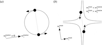This is consistent with the trends observed in figure 12 and with our argument (§ 3.1) that inertia causes particles to be ejected from high rotation regions of the flow. We expect that two particles in a high rotation region will experience small relative velocities parallel to the particle separation vector and large relative velocities perpendicular to the particle separation vector, as suggested by figure 14(a). We also expect that the parallel relative velocities will increase as particles accumulate in straining regions of the flow as a result of their inertia, while the perpendicular relative velocities will decrease, as shown in figure 14(b). Interestingly, we observe an opposite trend in the parallel relative velocities at $r/{\it\eta}\sim 10$ . We notice that $S_{2\Vert ,St}^{p}/S_{2\Vert ,St=0}^{fp}$ is slightly below 1, indicating that inertial particles have smaller parallel relative velocities than fluid particles. While the reason for this trend is unclear, since $S_{2\Vert ,St}^{p}/S_{2\Vert ,St=0}^{fp}$ and $S_{2\Vert ,St}^{fp}/S_{2\Vert ,St=0}^{fp}$ are approximately equal here, it must be related in some way to preferential sampling effects. At the largest separations, the relative velocities for inertial and fluid particles become equivalent, as expected, indicating that preferential sampling effects vanish in this limit.

Figure 13.

The parallel (a,c) and perpendicular (b,d) relative velocity variances of inertial particles ( $S_{2\Vert }^{p}$ and $S_{2\bot }^{p}$ , solid lines) and of the fluid at inertial particle positions ( $S_{2\Vert }^{fp}$ and $S_{2\bot }^{fp}$ , dashed lines) for $R_{{\it\lambda}}=597$ . All quantities are normalized by the relative velocity variances of $St=0$ particles. $St=0.05$ results are shown in (a,b), and $St=0.2$ results are shown in (c,d).

For $St=0.2$ , the particle relative velocities are much larger than the underlying fluid velocity differences at small separations, as is evident in figure 13(c,d). This difference is due to path-history effects (see Bragg & Collins Reference Bragg and Collins2014a ,Reference Bragg and Collins b ). That is, as inertial particles approach each other, they retain a memory of more energetic turbulence scales along their path histories, leading to relative velocities that exceed the local fluid velocity difference. These path-history effects imply that inertial particles can come together from different regions in the flow, occupy the same position in the flow at the same time and yet have different velocities due to their differing path histories. This effect is referred to as ‘caustics’, ‘crossing trajectories’ or ‘the sling effect’, causes a departure from $r^{2}$ -scaling in the second-order structure functions at small separations and can lead to large relative velocities (Yudine Reference Yudine1959; Falkovich et al. Reference Falkovich, Fouxon and Stepanov2002; Wilkinson & Mehlig Reference Wilkinson and Mehlig2005; Wilkinson et al. Reference Wilkinson, Mehlig and Bezuglyy2006; Falkovich & Pumir Reference Falkovich and Pumir2007). (Also note that while caustics are instantaneous events, the statistical manifestation of caustics is known as ‘random, uncorrelated motion’ and is discussed in IJzermans, Meneguz & Reeks (Reference IJzermans, Meneguz and Reeks2010).) Since the time scale over which the particles retain a memory of their interactions with turbulence increases with increasing inertia, caustics become more prevalent as $St$ increases.

Figure 14.

An illustration of the effect of preferential sampling on the parallel relative velocity $w_{\Vert }$ and the perpendicular relative velocity $w_{\bot }$ . In (a), two particles are in a rotating region of the flow. In this case, $w_{\Vert }$ is small and $w_{\bot }$ is large. In (b), the particles have been ejected from the rotating region as a result of their inertia and are in a straining region of flow. The two particles have a small value of $w_{\bot }$ and a large value of $w_{\Vert }$ .

One effect of caustics is to make the parallel and perpendicular relative velocity components nearly the same in the dissipation range, as can be seen in figure 12(c) for $St\gtrsim 0.3$ . (Note that fluid particles do not experience caustics and have $2S_{2\Vert }^{p}=S_{2\bot }^{p}$ for $r/{\it\eta}\ll 1$ as a result of continuity (e.g. see Pope Reference Pope2000).) For $St\geqslant 10$ , the relative velocities are almost unaffected by the underlying turbulence in the dissipation range. As a result, the relative velocities are nearly independent of $r/{\it\eta}$ in this range.

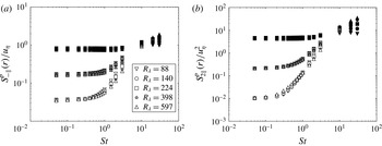
The effect of caustics can also be clearly seen in figure 15, where we plot the parallel relative velocities at a given separation as a function of $St$ . From this figure, it is evident that the particle relative velocities at the smallest separation sharply increase as $St$ exceeds approximately 0.2. The rapid increase in the particle relative velocities with $St$ is consistent with the notion that caustics take an activated form (Wilkinson et al. Reference Wilkinson, Mehlig and Bezuglyy2006) and that they are negligible below a critical value of $St$ (IJzermans et al. Reference IJzermans, Meneguz and Reeks2010; Salazar & Collins Reference Salazar and Collins2012b ). Our data suggest a critical Stokes number for caustics of approximately 0.2–0.3, in agreement with Falkovich & Pumir (Reference Falkovich and Pumir2007) and Salazar & Collins (Reference Salazar and Collins2012b ). The increase in the relative velocities occurs at higher values of $St$ as the separation increases. In this case, the particles are subjected to larger-scale turbulence, and hence the particles must have more inertia for their motion to deviate significantly from that of the underlying flow.

Figure 15.

(a) The mean inward relative velocities and (b) the relative velocity variances, plotted as a function of $St$ for small separations and different values of $R_{{\it\lambda}}$ . Open symbols denote $r=0.25{\it\eta}$ , grey filled symbols denote $r=1.75{\it\eta}$ and black filled symbols denote $r=9.75{\it\eta}$ .

We now examine the Reynolds-number dependence of the relative velocities, restricting our attention to the component parallel to the separation vector. From figure 15, we see that the relative velocities of the largest particles ( $St\gtrsim 10$ ) increase strongly with increasing $R_{{\it\lambda}}$ . There are two reasons for this trend. The first is that the effect of filtering on the larger turbulence scales decreases as $R_{{\it\lambda}}$ is increased (see § 3.2). The second is that $u^{\prime }/u_{{\it\eta}}$ increases with increasing $R_{{\it\lambda}}$ , indicating that large- $St$ particles in the dissipation range carry a memory of increasingly energetic turbulence (relative to the Kolmogorov scales) in their path history as $R_{{\it\lambda}}$ is increased.

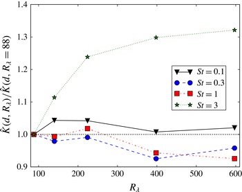
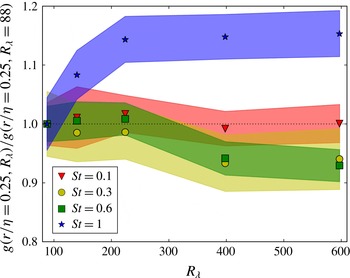
For smaller values of $St$ ( $St\leqslant 3$ ), the relative velocities in figure 15 are only weakly dependent on $R_{{\it\lambda}}$ , in agreement with previous DNS studies (Wang et al. Reference Wang, Wexler and Zhou2000; Bec et al. Reference Bec, Biferale, Cencini, Lanotte and Toschi2010a ; Onishi, Takahashi & Vassilicos Reference Onishi, Takahashi and Vassilicos2013; Rosa et al. Reference Rosa, Parishani, Ayala, Grabowski and Wang2013; Onishi & Vassilicos Reference Onishi and Vassilicos2014) and the model of Pan & Padoan (Reference Pan and Padoan2010). 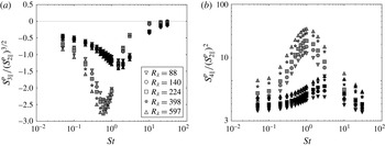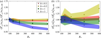To highlight any small Reynolds-number effects in this range, we therefore divide the relative velocities at $r=0.25{\it\eta}$ and a certain $R_{{\it\lambda}}$ by their value at $R_{{\it\lambda}}=88$ and plot the results in figure 16. We have included 95 % confidence intervals about the predicted values to provide an indication of the statistical significance of these weak Reynolds-number effects.

Figure 16.

(a) The mean inward relative velocities and (b) the relative velocity variances, plotted as function of $R_{{\it\lambda}}$ . The relative velocities are shown at $r/{\it\eta}=0.25$ , and the quantities at a given Reynolds number are divided by their corresponding value at $R_{{\it\lambda}}=88$ . Shaded contours denote 95 % confidence intervals about the sample mean.

For $St=0.3$ , the relative velocity variances increase weakly with increasing $R_{{\it\lambda}}$ (see figure 16 b). As $R_{{\it\lambda}}$ increases, the range of velocity scales $u^{\prime }/u_{{\it\eta}}$ increases, allowing some particle pairs in this Stokes-number range to sample more energetic turbulence as they converge to small separations, and causing the relative velocity variances to increase with increasing Reynolds number. Furthermore, turbulence intermittency, which also increases with increasing Reynolds number, may also contribute to the trend in the relative velocity statistics. We note that the mean inward velocities (figure 16 a) are less affected by changes in Reynolds number, presumably because the mean inward velocity is a lower-order statistic that is less influenced by the relatively rare events described above.

For $St=3$ , we also expect the increased scale separation, the increased intermittency of the turbulence or both to act to increase the relative velocities. However, we observe an overall decrease in the relative velocities with increasing $R_{{\it\lambda}}$ here, in agreement with Bec et al. (Reference Bec, Biferale, Cencini, Lanotte and Toschi2010a ), Rosa et al. (Reference Rosa, Parishani, Ayala, Grabowski and Wang2013). These reduced relative velocities are likely linked to the decrease in the Lagrangian rotation time scales $T_{\unicode[STIX]{x1D619}\unicode[STIX]{x1D619}}^{p}/{\it\tau}_{{\it\eta}}$ with increasing $R_{{\it\lambda}}$ observed in § 3.1. That is, as $T_{\unicode[STIX]{x1D619}\unicode[STIX]{x1D619}}^{p}/{\it\tau}_{{\it\eta}}$ decreases with increasing $R_{{\it\lambda}}$ , the particles have a shorter memory of fluid velocity differences along their path histories, which in turn causes the relative velocities to decrease.

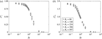
We now examine the behaviour of the scaling exponents of $S_{-\Vert }^{p}\propto r^{{\it\zeta}_{\Vert }^{-}}$ and $S_{2\Vert }^{p}\propto r^{{\it\zeta}_{\Vert }^{2}}$ at small separations. (These scaling exponents will also be used in § 4.2 to understand and predict the trends in the particle clustering.) We compute ${\it\zeta}_{\Vert }^{-}$ and ${\it\zeta}_{\Vert }^{2}$ using a linear least-squares regression for $0.75\leqslant r/{\it\eta}\leqslant 2.75$ at different values of $St$ and $R_{{\it\lambda}}$ . Note that while using such a large range of $r/{\it\eta}$ will necessarily introduce finite-separation effects, there is generally too much noise in the data to accurately compute the scaling exponents over smaller separations.

The scaling exponents are plotted in figure 17. We note that the scaling exponents are below those predicted by Kolmogorov (Reference Kolmogorov1941) (hereafter ‘K41’) for fluid ( $St=0$ ) particles ( ${\it\zeta}_{\Vert }^{-}=1$ and ${\it\zeta}_{\Vert }^{2}=2$ ) and, like the relative velocities themselves, vary only slightly as $R_{{\it\lambda}}$ changes.

Figure 17.

Dissipation range scaling exponents for $S_{-\Vert }^{p}$ (a) and $S_{2\Vert }^{p}$ (b) for various values of $St$ and $R_{{\it\lambda}}$ . The exponents are computed from linear least-squares regression for $0.75\leqslant r/{\it\eta}\leqslant 2.75$ .

For $St\geqslant 10$ , the scaling exponents are approximately zero, indicating that the relative velocities are generally independent of $r$ , as explained above. The scaling exponents for $1\lesssim St\lesssim 3$ generally increase with increasing $R_{{\it\lambda}}$ , since path-history interactions (which generally decrease the scaling exponents) become less important, as explained above. Finally, we note that ${\it\zeta}_{\Vert }^{2}$ decreases with increasing $R_{{\it\lambda}}$ for $St\lesssim 1$ , since intermittent path-history effects are expected to be more important here.

We next consider the PDFs of the relative velocities in the dissipation range. Figure 18 shows the PDFs for $0\leqslant r/{\it\eta}\leqslant 2$ and $R_{{\it\lambda}}=597$ . In figure 18(a), we see that as $St$ increases, the tails of the PDF of $w_{\Vert }^{p}/u_{{\it\eta}}$ become more pronounced, indicating that larger relative velocities become more frequent, in agreement with our observations above.

Figure 18.

PDFs of the particle relative velocities $w_{\Vert }^{p}$ for separations $0\leqslant r/{\it\eta}\leqslant 2$ and $R_{{\it\lambda}}=597$ . The relative velocities are normalized by both $u_{{\it\eta}}$ (a) and $(S_{2\Vert }^{p})^{1/2}$ (b). The solid lines denote the relative velocity PDFs for $St=0$ particles, and the dotted line in (b) indicates a standard normal distribution.

We show PDFs in standardized form in figure 18(b) to analyse the extent to which they deviate from that of a Gaussian distribution. It is evident that the degree of non-Gaussianity peaks for $St\sim 1$ and becomes smaller as $St$ increases. The physical explanation for this intermittency at $St\sim 1$ is that the motion of these particles is affected by both the small-scale underlying turbulence and by the particles’ memory of large-scale turbulent events in their path histories. This combination of contributions from both large- and small-scale events leads to strong intermittency. We also see that the underlying fluid is itself quite intermittent at this small separation, as expected (e.g. see Gotoh, Fukayama & Nakano Reference Gotoh, Fukayama and Nakano2002).

We now use three statistical measures to quantify the shape of the PDFs. The first is the ratio between the mean inward relative velocities and the standard deviation of the relative velocities, $S_{-\Vert }^{p}/(S_{2\Vert }^{p})^{1/2}$ ; the second is the skewness of the relative velocities, $S_{3\Vert }^{p}/(S_{2\Vert }^{p})^{3/2}$ ; and the third is the kurtosis of the relative velocities, $S_{4\Vert }^{p}/(S_{2\Vert }^{p})^{2}$ . (Due to insufficient statistics, we will not consider data from these latter two quantities for $r/{\it\eta}<1.75$ .)

We show the ratio $S_{-\Vert }^{p}/(S_{2\Vert }^{p})^{1/2}$ in figure 19. One motivation for looking at this ratio is that existing theories (e.g. see Zaichik et al. Reference Zaichik, Simonin and Alipchenkov2003; Pan & Padoan Reference Pan and Padoan2010) only predict the relative velocity variance, and by assuming the relative velocities have a Gaussian distribution, relate this variance to the mean inward relative velocity. For a Gaussian distribution, this ratio is approximately 0.4. At all values of $St$ , $R_{{\it\lambda}}$ and $r/{\it\eta}$ , our data indicate that the ratio is below 0.4 and thus that the particle relative velocities are intermittent (see also Wang et al. Reference Wang, Wexler and Zhou2000; Pan & Padoan Reference Pan and Padoan2013). The degree of intermittency peaks for order unity $St$ , high $R_{{\it\lambda}}$ and small $r/{\it\eta}$ , and using a Gaussian prediction in this regime would lead to predictions of the mean inward velocity which are in error by more than a factor of 2.

Figure 19.

The ratio between mean inward relative velocities and the standard deviation of the relative velocities as a function of $St$ for small separations and different values of $R_{{\it\lambda}}$ . Open symbols denote $r=0.25{\it\eta}$ , grey filled symbols denote $r=1.75{\it\eta}$ , and black filled symbols denote $r=9.75{\it\eta}$ . The horizontal dotted line indicates that value of this quantity for a Gaussian distribution.

We next consider the skewness, $S_{3\Vert }^{p}/(S_{2\Vert }^{p})^{3/2}$ , to provide information about the asymmetry of the relative velocities. Figure 20(a) indicates that the relative velocities are negatively skewed (Wang et al. Reference Wang, Wexler and Zhou2000; Ray & Collins Reference Ray and Collins2011). This skewness is a result of two contributions. First, the velocity derivatives of the underlying turbulence are negatively skewed, a consequence of the energy cascade (Tavoularis, Bennett & Corrsin Reference Tavoularis, Bennett and Corrsin1978). Second, additional skewness arises from the path-history effect described earlier (see also Bragg & Collins Reference Bragg and Collins2014b ). Figure 20(a) shows by implication that at $St\sim 1$ it is the latter effect that dominates the skewness behaviour. At even larger values of $St$ , the effect of both mechanisms decreases because, with increasing Stokes number, the particle velocity dynamics becomes increasingly decoupled from the small-scale fluid velocity field and their motion becomes increasingly ballistic in the dissipation range.

Figure 20.

The (a) skewness and (b) kurtosis of the relative velocities as a function of $St$ for separations in the dissipation range and different values of $R_{{\it\lambda}}$ . Grey filled symbols denote $r=1.75{\it\eta}$ , and black filled symbols denote $r=9.75{\it\eta}$ .

Finally, we consider the kurtosis of the relative velocities, $S_{4\Vert }^{p}/(S_{2\Vert }^{p})^{2}$ , in figure 20(b) to quantify the contributions from intermittent events in the tails of the PDFs. The trends are similar to those in $S_{-\Vert }^{p}/(S_{2\Vert }^{p})^{1/2}$ , as expected, indicating that contributions from intermittent events become strongest for intermediate $St$ , the smallest separations and the highest Reynolds numbers. In all cases, the kurtosis is above that for a Gaussian distribution ( $S_{4\Vert }^{p}/(S_{2\Vert }^{p})^{2}=3$ ).

Finally we close this section with two comments. We first note that the recent study by Saw et al. (Reference Saw, Bewley, Bodenschatz, Ray and Bec2014) that compares experimentally measured relative velocities of inertial particles with DNS found that while the Stokes drag model is able to capture all of the qualitative trends observed in the experiments, it is unable to provide quantitative predictions for the tails of the relative velocity PDFs, suggesting that some of the neglected terms in the Maxey & Riley (Reference Maxey and Riley1983) particle equation of motion may be required to yield quantitatively correct higher-order relative velocity statistics.

The second comment is related to the inertial range structure functions. It is a common practice to report the power-law exponents of higher-order velocity structure functions for fluid particles (e.g. see Kerr, Meneguzzi & Gotoh Reference Kerr, Meneguzzi and Gotoh2001; Gotoh et al. Reference Gotoh, Fukayama and Nakano2002; Shen & Warhaft Reference Shen and Warhaft2002; Ishihara et al. Reference Ishihara, Gotoh and Kaneda2009). Salazar & Collins (Reference Salazar and Collins2012b ) reported the corresponding exponents for inertial particles. However, as shown by Bragg, Ireland & Collins (Reference Bragg, Ireland and Collins2015), in a turbulent flow with infinite Reynolds number, and $r/{\it\eta}\gg St^{3/2}$ , the inertial particle structure functions reduce to those of fluid particles. Yet for those same particles in the range $1\ll r/{\it\eta}\ll St^{3/2}$ , inertial effects cause systematic deviations between inertial particle and fluid particle structure functions. The existence of two scaling regions for inertial particles in high-Reynolds-number turbulence implies that no single exponent can capture the entire inertial range. Thus, the results reported in Salazar & Collins (Reference Salazar and Collins2012b ) are most likely an artefact of the relatively low Reynolds number of the study ( $R_{{\it\lambda}}\leqslant 120$ ).

4.2 Particle clustering

As discussed in § 1, inertial particles form clusters when placed in a turbulent flow. We first consider a theoretical framework for understanding this clustering (§ 4.2.1), and then analyse the clustering using DNS (§ 4.2.2).

4.3 Collision kernel

We now consider the kinematic collision kernel $K$ for inertial particles, which has been shown to depend on both the radial distribution function and the radial relative velocities,

where $d$ is the particle diameter (see Sundaram & Collins Reference Sundaram and Collins1997; Wang, Wexler & Zhou Reference Wang, Wexler and Zhou1998). While we simulate only point particles (refer to § 2.2), we compute $d$ from $St$ by assuming a given ${\it\rho}_{p}/{\it\rho}_{f}$ . To study the dependence of $K(d)$ on ${\it\rho}_{p}/{\it\rho}_{f}$ , we consider three different values for this parameter: 250, 1000 and 4000. (Note that for droplets in atmospheric clouds, ${\it\rho}_{p}/{\it\rho}_{f}\approx 1000$ .)

In general, we do not have adequate statistics to calculate $g(r)$ or $S_{-\Vert }^{p}(r)$ at $r=d$ at low values of $St$ ( $St\leqslant 3$ for ${\it\rho}_{p}/{\it\rho}_{f}=250$ and 1000 and $St\leqslant 10$ for ${\it\rho}_{p}/{\it\rho}_{f}=4000$ ) and so we extrapolate from the power-law fits in §§ 4.1 and 4.2.2 down to these separations, as was also done in Rosa et al. (Reference Rosa, Parishani, Ayala, Grabowski and Wang2013). For larger $St$ ( $St\geqslant 10$ for ${\it\rho}_{p}/{\it\rho}_{f}=250$ and 1000 and $St\geqslant 20$ for ${\it\rho}_{p}/{\it\rho}_{f}=4000$ ), the particle diameters are sufficiently large such that we can compute $g(d)$ and $S_{-\Vert }^{p}(d)$ by interpolating between data at smaller and larger separations.

Following Voßkuhle et al. (Reference Voßkuhle, Pumir, Lévêque and Wilkinson2014), we compute the non-dimensional collision kernel $\hat{K}(d)\equiv K(d)/(d^{2}u_{{\it\eta}})=4{\rm\pi}g(d)S_{-\Vert }^{p}(d)/u_{{\it\eta}}$ . Figure 25 shows $\hat{K}(d)$ for different values of ${\it\rho}_{p}/{\it\rho}_{f}$ . Results from Rosa et al. (Reference Rosa, Parishani, Ayala, Grabowski and Wang2013) (deterministic forcing scheme, no gravity, ${\it\rho}_{p}/{\it\rho}_{f}=1000$ ) are included in the inset to figure 25.

Figure 25.

The non-dimensional collision kernel $\hat{K}(d)$ as a function of $St$ for different values of $R_{{\it\lambda}}$ . Data are shown for ${\it\rho}_{p}/{\it\rho}_{f}=250$ (filled black symbols), ${\it\rho}_{p}/{\it\rho}_{f}=1000$ (open symbols) and ${\it\rho}_{p}/{\it\rho}_{f}=4000$ (filled grey symbols). Legend entries marked with $\dagger$ indicate data taken from Rosa et al. (Reference Rosa, Parishani, Ayala, Grabowski and Wang2013) (deterministic forcing scheme, no gravity) at ${\it\rho}_{p}/{\it\rho}_{f}=1000$ . These data are only included in the inset, where they are compared with our results at ${\it\rho}_{p}/{\it\rho}_{f}=1000$ .

For $St\geqslant 10$ , the collision kernels increase strongly with increasing $R_{{\it\lambda}}$ , since both the relative velocities and the RDFs increase with $R_{{\it\lambda}}$ here (see §§ 4.1 and 4.2.2). $\hat{K}(d)$ is also independent of ${\it\rho}_{p}/{\it\rho}_{f}$ here. The physical explanation is that while changes in ${\it\rho}_{p}/{\it\rho}_{f}$ lead to changes in $d$ , $S_{-\Vert }^{p}(d)/u_{{\it\eta}}$ and $g(d)$ are largely independent of $d$ here (see §§ 4.1 and 4.2.2).

Such particles, however, are generally above the size range of droplets in atmospheric clouds (e.g. see Ayala et al. Reference Ayala, Rosa, Wang and Grabowski2008), and thus our primary focus is on the collision rates of smaller ( $St\lesssim 3$ ) particles. $\hat{K}(d)$ is independent of ${\it\rho}_{p}/{\it\rho}_{f}$ for $1\lesssim St\leqslant 3$ , in agreement with the findings of Voßkuhle et al. (Reference Voßkuhle, Pumir, Lévêque and Wilkinson2014). In this case, while both $g(d)$ and $S_{-\Vert }^{p}/u_{{\it\eta}}$ are dependent on $d$ , these two quantities have opposite scalings (see § 4.2.2), causing their product to be independent of $d$ (and thus of ${\it\rho}_{p}/{\it\rho}_{f}$ ).

For $St\lesssim 3$ , our data show very little effect of $R_{{\it\lambda}}$ on the collision rates, and are in good agreement with the collision statistics from Rosa et al. (Reference Rosa, Parishani, Ayala, Grabowski and Wang2013) at ${\it\rho}_{p}/{\it\rho}_{f}=1000$ (shown in the inset to figure 25). However, since the Reynolds numbers in clouds ( $R_{{\it\lambda}}\sim 10\,000$ ) are at least an order of magnitude larger than those in the DNS, it is important to discern even weak trends in the collision kernel with the Reynolds number. We therefore plot the ratio of $\hat{K}(d)$ at a given Reynolds number to that at $R_{{\it\lambda}}=88$ for $St\leqslant 3$ in figure 26.

Figure 26.

The ratio between $\hat{K}(d)$ at a given value of $R_{{\it\lambda}}$ to that at $R_{{\it\lambda}}=88$ , to highlight any Reynolds-number effects for $St\leqslant 3$ . All data correspond to ${\it\rho}_{p}/{\it\rho}_{f}=1000$ .

For $St\leqslant 1$ , the collision statistics are almost completely independent of $R_{{\it\lambda}}$ . This Reynolds-number independence is expected at $St=0.1$ and $St=0.3$ , since both $S_{-\Vert }^{p}/u_{{\it\eta}}$ and $g$ are independent of $R_{{\it\lambda}}$ here (refer to §§ 4.1 and 4.2.2). For $St=1$ , $S_{-\Vert }^{p}/u_{{\it\eta}}$ decreases with increasing $R_{{\it\lambda}}$ (see § 4.1), while $g$ increases with increasing $R_{{\it\lambda}}$ (see § 4.2.2). These two trends apparently offset each other, causing the collision kernel to be essentially independent of Reynolds number at $St=1$ . Finally, for $St=3$ , the collision kernel increases weakly as $R_{{\it\lambda}}$ increases. In this case, the increase in the RDFs with increasing $R_{{\it\lambda}}$ (§ 4.2.2) more than compensates for the decrease in the relative velocities (§ 4.1), causing the collision kernel to increase weakly.

These findings suggest that lower-Reynolds-number studies may in fact capture the essential physics responsible for droplet collisions in highly turbulent clouds. However, the results must be interpreted with caution for two reasons. First, the collision rates for $St\leqslant 3$ were computed by extrapolating power-law fits to very small separations, and it is not known if the functional form of the relative velocities and the RDFs remains the same at these separations. Second, even the highest Reynolds numbers in this study are still at least an order of magnitude smaller than those in atmospheric clouds. It is thus possible that the turbulence could exhibit different characteristics at much higher Reynolds numbers, or that the above trends in the Reynolds number, though weak, could lead to substantially different collision rates when $R_{{\it\lambda}}$ is increased by another order of magnitude.