



1. Introduction
The random structure considered in this paper is well represented by an urn model. We randomly distribute indistinguishable balls over distinguishable urns. Each urn has a size, which controls the probability of a ball put into the urn. An urn is divided if it is replaced by two urns whose total size equals that of the divided urn. Conversely, two urns are merged if they are replaced by one urn whose size equals the total size of merged urns. Any combination of division and merger is called resizing.
The distribution of balls over urns is closed under resizing if it is unchanged after resizing. For example, let us regard the marginal parameter (cell probability) of the multinomial distribution as the size of an urn. Then the multinomial distribution is closed under infinite resizing, as we will see.
The multinomial distribution possesses many good features due to this closure property. However, it cannot control second moments, which is a classical motivation to generalize the multinomial distribution. We will see some existing approaches for the generalization in subsequent sections, yet unlike them, our study generalizes the multinomial distribution so that the closure property remains.
The present article is organized as follows. Section 1.1 introduces notation and the Bell polynomials of [Reference Comtet11]. Section 2 characterizes a family of generalized multinomial distribution closed under resizing. This family is called the Bell polynomial distribution (BPD) because its probability mass is expressed using the Bell polynomial. The BPD can be obtained by conditioning random frequencies that have an infinitely divisible distribution; a distribution is infinitely divisible if and only if it equals the distribution of the sum of infinitely many independent and identically distributed (i.i.d.) random variables. Section 3 derives the marginal properties of the BPD such as moments, exploiting the closure property. Section 4 considers the case of random sizes, which includes the mixture of the BPD with the Dirichlet distribution, with implications to Bayesian inference. An important generalization of the Dirichlet distribution is the normalized infinitely divisible (NID) distribution proposed by [Reference Favaro, Hadjicharalambous and Prünster21]. It turns out that the mixed multinomial distribution with a NID distribution equals the BPD. Section 5 examines two examples of the BPD, one of which is the Dirichlet multinomial mixture. Section 6 shows the existence of a stochastic process such that the finite-dimensional distribution is the BPD. This fact leads to a limiting argument to obtain a random partitioning distribution of a positive integer. The present study ends with Section 7. Proofs are collected in the Appendix.
1.1. Notation and Bell polynomials
This subsection sets up notation and summarizes some properties of the Bell polynomials to be used. For a recent review of Bell polynomials, see [Reference Qi, Niu, Lim and Yao45].
We denote the set of positive integers and the set of non-negative integers by
 $\mathbb{N}$
and
 $\mathbb{N}_0$
, respectively. The set of positive real numbers is denoted by
 $\mathbb{R}_+$
. Similarly,
 $\mathbb{R}_-$
denotes the set of negative real numbers, and
 $\mathbb{R}$
denotes the set of real numbers. Also,
 $\mathbb{R}_{0+} \, :\!= \, \{0\}\cup \mathbb{R}_+$
and
 $\mathbb{R}_{0-} \, :\!= \, \{0\}\cup \mathbb{R}_-$
.
For
 $n\in \mathbb{N}$
, let
 $\boldsymbol{w}_n \, :\!= \, (w_1,w_2,\ldots,w_n)\in \mathbb{R}^n$
. Then partial Bell polynomials are defined for
 $k\in [n] \, :\!= \, \{1,2,\ldots,n\}$
as
 \[B_{n,k}(\boldsymbol{w}_n) \, :\!= \, n!\sum_{(s_1,\ldots,s_n)\in {\mathcal{P}}_{n,k}}\prod_{i=1}^n\biggl( \dfrac{{w_i}}{i!}\biggr)^{s_i}\dfrac{1}{s_i!},\]
where
 \[{\mathcal{P}}_{n,k} \, :\!= \, \Biggl\{(s_1,\ldots,s_n)\colon s_i\in \mathbb{N}_0,\ i\in\mathbb{N},\ \sum_{i=1}^n is_i=n,\sum_{i=1}^n s_i=k\Biggr\}.\]
Considering this definition,
 $B_{n,1}(\boldsymbol{w}_n)=w_n$
, and
 $B_{n,n}(\boldsymbol{w}_n)=w_1^n$
. In fact,
 $B_{n,k}(\boldsymbol{w}_n)$
does not depend on
 $w_i,\ i>n-k+1$
.
The partial Bell polynomial is sometimes called the Bell polynomial of the second kind. The first kind or the total Bell polynomial
 $B_n(\boldsymbol{w}_n)$
is defined as the sum of partial Bell polynomials over k. Namely,
 \[B_n(\boldsymbol{w}_n) \, :\!= \, n!\sum_{(s_1,\ldots,s_n)\in {\mathcal{P}}_{n}}\prod_{i=1}^n\biggl(\dfrac{{w_i}}{i!}\biggr)^{s_i}\dfrac{1}{s_i!},\]
where
 ${\mathcal{P}}_{n} \, :\!= \, \bigcup_{k=1}^n{\mathcal{P}}_{n,k}$
. It is important that
 $B_0(\! \cdot \!)=B_{0,0}(\! \cdot \!)\equiv 1$
; see e.g. [Reference Riordan46]. Conventionally,
 $B_{n,0}(\boldsymbol{w}_n)=0$
for
 $n\in \mathbb{N}$
.
For future use, we cite equation 11.3 of [Reference Charalambides8], namely
 \begin{equation}B_n(c w_1,c^2 w_2,\ldots,c^n w_n)=c^nB_n(\boldsymbol{w}_n).\end{equation}
In particular,
 \begin{equation}B_n(-w_1,(\!-\!1)^2 w_2,\ldots,(\!-\!1)^n w_n)=(\!-\!1)^nB_n(\boldsymbol{w}_n).\end{equation}
Also, from equation 11.15 of [Reference Charalambides8],
 \begin{equation}B_{n}(\lambda,\boldsymbol{w}_n) \, :\!= \, B_n(\lambda w_1,\lambda w_2,\ldots,\lambda w_n)=\sum_{k=1}^n \lambda^kB_{n,k}(\boldsymbol{w}_n).\end{equation}
Equation (1.3) implies that
 \begin{equation}B_{n}(\lambda,\boldsymbol{w}_n)=\lambda w_n+\boldsymbol{\mathrm{O}} (\lambda^2), \quad \lambda\to 0.\end{equation}
Also
 \begin{equation}B_{n}(\lambda,\boldsymbol{w}_n)=\lambda^n w_1^n+\boldsymbol{\mathrm{O}} (\lambda^{n-1}),\quad \lambda\to \infty .\end{equation}
In the following, the variables of the Bell polynomial are written as
 $\boldsymbol{w} \, :\!= \, (w_i)_{i\in \mathbb{N}}$
for simplicity and dealing with the sequence of Bell polynomials. We regard
 $B_{n,k}(\boldsymbol{w})$
as
 $B_{n,k}(\boldsymbol{w}_n)$
so that
 $B_n(w)=B_n(\boldsymbol{w}_n)$
.
Concerning an urn model, we denote the deterministic number of urns by
 $J\in \mathbb{N}$
. The total number of balls is deterministic and denoted by
 $n\in \mathbb{N}_0$
. The random number of balls in the jth urn is denoted by
 $F_j\in \mathbb{N}_0$
,
 $j\in [J]$
. The space of these frequencies
 $\boldsymbol{F}_J \, :\!= \, (F_1,F_2,\ldots,F_J)$
is denoted by
 \[{\mathcal{F}}_{n,J} \, :\!= \, \biggl\{\boldsymbol{f}_J \, :\!= \, (\,f_1,f_2,\ldots,f_J)\colon f_j\in \mathbb{N}_0,\ j\in[J],\ \sum_j f_j=n\biggr\}.\]
The size of the jth urn is denoted by
 $\lambda_j$
. The vector of the sizes is denoted by
 $\boldsymbol{\lambda}_J \, :\!= \, (\lambda_1,\lambda_2,\ldots,\lambda_J)$
. The total of the sizes is denoted by
 $\lambda_{\bullet}=\sum_{j=1}^J \lambda_j$
; the subscript ‘
 $\bullet$
’ expresses summing up over the index throughout the manuscript.
2. Generalization of the multinomial distribution
2.1. Construction
Vershik [Reference Vershik55] defines a multiplicative probability measure on
 ${\mathcal{P}}_n$
for a sequence of functions
 $(\tilde{h}_i\colon \mathbb{N}_0\mapsto\mathbb{R}_+)_{i=1}^\infty $
by the following probability mass function (PMF):
 \[p(\boldsymbol{s}_n)=\prod_{i=1}^n\tilde{h}_i(s_i)/Q_n,\ \boldsymbol{s}_n\in{\mathcal{P}}_n,\]
where
 $Q_n=\sum_{\boldsymbol{s}_n\in {\mathcal{P}}_n}\prod_{i=1}^n\tilde{h}_i(s_i)$
is a normalizing constant. In this family, a margin is not independent from other margins, but the multiplicative form of the probability mass simplifies the combinatorial structure of the family.
Analogously, we can define a multiplicative probability measure on
 ${\mathcal{F}}_{n,J}$
for a sequence of functions
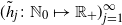 $(\tilde{h}_j\colon \mathbb{N}_0\mapsto\mathbb{R}_+)_{j=1}^\infty $
by the following PMF:
 \begin{equation}p(\,\boldsymbol{f}_{J})=\prod_{j=1}^J\tilde{h}_j(\,f_j)/Q_{n,J},\quad \boldsymbol{f}_J\in{\mathcal{F}}_{n,J},\end{equation}
where
 $Q_{n,J}=\sum_{\boldsymbol{f}_J\in{\mathcal{F}}_{n,J}}\prod_{j=1}^J\tilde{h}_j(\,f_j)$
is a normalizing constant.
For example, if
 $\tilde{h}_j(\,f_j)=\lambda_j^{f_j}/f_j!$
then
 $Q_{n,J}=\lambda_{\bullet}^n/n!$
in (2.1). This case
 \begin{equation}p(\,\boldsymbol{f}_J)=\dfrac{n!}{\lambda_{\bullet}^n}\prod_{j=1}^J\dfrac{\lambda_j^{f_j}}{f_j!},\quad \boldsymbol{f}_J\in{\mathcal{F}}_{n,J},\end{equation}
defines the multinomial distribution, which is usually parameterized by a cell probability or
 $\pi_j \, :\!= \, \lambda_j/\lambda_{\bullet},\ j\in [J]$
. Because
 $\lambda_J=\lambda_{\bullet}-\sum_{j=1}^{J-1}\lambda_j$
, this reparameterization is expressed as
 \begin{equation}\boldsymbol{\lambda}_J\mapsto(\pi_1,\pi_2,\ldots,\pi_{J-1},\lambda_{\bullet}).\end{equation}
However, for notational convenience, we denote the transformed parameters by
 $(\boldsymbol{\pi}_J;\ \lambda_{\bullet})$
, where
 $\boldsymbol{\pi}_J \, :\!= \, (\pi_1,\pi_2,\ldots,\pi_J)$
. The
 $(J-1)$
-dimensional multinomial distribution (2.2) reparameterized by (2.3) is referred to by
 $\mathtt{Mn}_J(n,\boldsymbol{\pi}_J)$
, which does not depend on
 $\lambda_{\bullet}$
.
We regard the space of cell probabilities as the
 $(J-1)$
-dimensional unit simplex
 \[\triangle^{J-1} \, :\!= \, \Biggl\{\boldsymbol{\pi}_J\colon \sum_{j=1}^J\pi_j=1,\ \pi_j\in \mathbb{R}_+,\ j\in[J]\Biggr\}.\]
It is important that
 $\pi_j$
is strictly positive in this definition. If
 $\pi_j=0$
then the observed
 $F_j$
is almost surely zero, which is called structural zero in statistics. By excluding structural zeros, we avoid indeterminate J. Also, as a result, the support of
 $\mathtt{Mn}_J(n,\boldsymbol{\pi}_J)$
does not degenerate from
 ${\mathcal{F}}_{n,J}$
. Namely,
 \begin{equation}\text{for all }\boldsymbol{f}_J\in {\mathcal{F}}_{n,J},\quad p(\,\boldsymbol{f}_J)>0.\end{equation}
We fix the space of cell probabilities to
 $\triangle^{J-1}$
. Then the corresponding space of
 $\boldsymbol{\lambda}_J$
can only be
 $\mathbb{R}_+^J$
or
 $\mathbb{R}_-^J$
. However, the negative size of an urn is difficult to interpret. Hence, for the time being, we assume that
 $\lambda_j\in \mathbb{R}_+$
,
 $ j\in [J]$
.
The multinomial distribution
 $\mathtt{Mn}_J(n,\boldsymbol{\pi}_J)$
is the n-fold convolution of i.i.d. samples of
 $\mathtt{Mn}_J(1,\boldsymbol{\pi}_J)$
. Consequently, (2.2) is invariant under the permutation of n samples. This property is called the exchangeability of balls.
We note that (2.2) is also invariant under the permutation of urns. The jth urn has two attributes: a size
 $\lambda_j$
and the number of balls
 $f_j$
in the urn. Permuting urns exchanges
 $(\,f_j;\ \lambda_j)$
with
 $(\,f_i;\ \lambda_i)$
,
 $ i\neq j$
, by which the right-hand side of (2.2) is unchanged. We call this property the exchangeability of urns.
It is noteworthy that exchangeability often refers to that of arguments of a function. For example, if all
 $\lambda_j$
are equal then
 $p(\ldots,f_i,\ldots,f_j,\ldots)=p(\ldots,f_j,\ldots,f_i,\ldots)$
,
 $ i\neq j$
, for (2.2). This
 $p(\! \cdot \!)$
is thus called exchangeable, but the exchangeability of urns is a different concept since it holds for unequal
 $\lambda_j$
.
We would like to generalize the multinomial distribution so that the closure property under resizing remains. Since resizing operates on urns, the closure property seems relevant to the exchangeability of urns. Hence we retain it but neglect the exchangeability of balls.
We note another characteristic of (2.2), that the normalizing constant
 $\lambda_{\bullet}^n/n!$
has the same functional form as that of the marginal numerator
 $\lambda_j^{f_j}/f_j!$
. This symmetry between the numerator and the denominator is actually the source of the closure property.
Consequently, we consider a subfamily of (2.1) with constraints
 $\tilde{h}_j(\,f_j)=h(\,f_j;\ \lambda_j)/f_j!$
and
 $Q_{n,J}=h(n;\ \lambda_{\bullet})/n!$
. Namely,
 $h(\! \cdot \!)$
is restricted to satisfy
 \begin{equation}\sum_{\boldsymbol{f}_J\in {\mathcal{F}}_{n,J}}p(\,\boldsymbol{f}_J)=1\end{equation}
under
 \begin{equation}p(\,\boldsymbol{f}_J)=\dfrac{n!}{h(n;\ \lambda_{\bullet})}\prod_{j=1}^J\dfrac{h(\,f_j;\ \lambda_j)}{f_j!},\quad \boldsymbol{f}_J\in{\mathcal{F}}_{n,J}.\end{equation}
To determine the form of
 $h(\! \cdot \!)$
, we additionally assume continuity of
 $h(\cdot;\ \lambda)$
as follows.
Definition 2.1. The PMF (2.6) that satisfies the following three conditions for
 $n\in \mathbb{N}_0$
,
 $J\in \mathbb{N}$
, and
 $\boldsymbol{\lambda}_J\in \mathbb{R}_+^J$
defines a family of distributions denoted by
 ${\mathcal{M}}$
.
-
(i) Positivity. The PMF is strictly positive as in (2.4).
-
(ii) Unity. The total of probabilities is unity as in (2.5).
-
(iii) Continuity.
 $h(\,f;\ \lambda)$
is continuous in
$\lambda$
for
$f\in \mathbb{N}_0$
.


Theorem 2.1 below shows that
 $h(\,f;\ \lambda)$
is uniquely determined by the sequence of
 $h(\,f;1)=h_f$
,
 $ f\in\mathbb{N}$
, for a member of
 ${\mathcal{M}}$
. Therefore
 $(h_f)_{f\in\mathbb{N}}$
can be regarded as a parameter vector. It is noteworthy that
 $h(0;1)$
leads to 1.
Theorem 2.1. For
 $(h_f)_{f\in\mathbb{N}} \in \mathbb{R}_+^\infty $
, define
 $h(\,f;\ \lambda)$
by equating the coefficient of
 $s^f$
on both sides of
 \begin{equation}\sum_{f=0}^\infty \dfrac{s^f}{f!}h(\,f;\ \lambda)=\Biggl(1+\sum_{f=1}^\infty \dfrac{s^f}{f!}h_f\Biggr)^\lambda.\end{equation}
Then the family of (2.6) is equivalent to
 ${\mathcal{M}}$
.
2.2. Characterization
The family
 ${\mathcal{M}}$
of Definition 2.1 is not very treatable when it is parameterized with
 $(h_f)_{f\in\mathbb{N}}$
. Hence we reparameterize it using Bell polynomials.
Theorem 2.2. Let
 $h_f=B_f(\boldsymbol{w})$
,
 $ f\in\mathbb{N}$
. Then, for all
 $n\in\mathbb{N}_0$
, (2.6) equals
 \begin{equation}p(\,\boldsymbol{f}_J)=\dfrac{n!}{B_n(\lambda_{\bullet}, \boldsymbol{w})}\prod_{j=1}^J\dfrac{B_{f_j}(\lambda_j,\boldsymbol{w})}{f_j!},\quad \boldsymbol{f}_J\in{\mathcal{F}}_{n,J}.\end{equation}
As a distribution on
 ${\mathcal{F}}_{n,J}$
, the parameter vector of (2.8) is
 $(\boldsymbol{\lambda}_J, \boldsymbol{w}_n)$
, where
 $\boldsymbol{w}_f$
consists of the first f entries of
 $\boldsymbol{w}_n$
. Nevertheless, the three conditions of Definition 2.1 must hold for all
 $n\in\mathbb{N}_0$
. Theorem 2.3 thus clarifies the space of
 $\boldsymbol{w}$
.
Theorem 2.3. The distribution (2.8) satisfies (2.4) for
 $n\in \mathbb{N}_0$
,
 $J\in \mathbb{N}$
, and
 $\boldsymbol{\lambda}_J\in \mathbb{R}_+^J$
if and only if
 $\boldsymbol{w}$
belongs to either
 $\mathbb{R}_+\times\mathbb{R}_{0+}^\infty \,=\!:\, \Omega_1$
or
 $\mathbb{R}_-\times\prod_{i=2}^\infty (\!-\!1)^i\mathbb{R}_{0+}\,=\!:\, \Omega_2$
, where
 $(\!-\!1)\mathbb{R}_{0+}=\mathbb{R}_{0-}$
.
When
 $\boldsymbol{\lambda}_J\in \mathbb{R}_-^J$
in Theorem 2.3,
 $\boldsymbol{w}$
belongs to either
 $\mathbb{R}_-\times\mathbb{R}_{0-}^\infty $
or
 $\mathbb{R}_+\times\prod_{i=2}^\infty (\!-\!1)^i\mathbb{R}_{0-}$
due to (1.2). Therefore only four parameter spaces of
 $(\boldsymbol{\lambda}_J,\boldsymbol{w})$
exist, but the distributional property of (2.8) is equivalent among them due to (1.2). Hence we restrict our attention to the most intuitive space
 $\mathbb{R}_+^J\times\Omega_1$
as in Definition 2.2.
Definition 2.2. Let
 $\boldsymbol{w}\in\Omega_1$
. For each
 $n\in \mathbb{N}_0$
, the distribution that has the PMF (2.8) for
 $J\in \mathbb{N}$
and
 $\boldsymbol{\lambda}_J\in \mathbb{R}_+^J$
is called the Bell polynomial distribution (BPD) of the nth order, which is referred to by
 $\mathtt{BP}_J(n,\boldsymbol{\lambda}_J;\,\boldsymbol{w})$
. The sequence of the BPD of finite orders generated by
 $\boldsymbol{w}$
constitutes a family
 $\{(\mathtt{BP}_J(n,\boldsymbol{\lambda}_J;\,\boldsymbol{w}))_{n\in \mathbb{N}_0}\colon \boldsymbol{w}\in \Omega_1\}$
denoted by
 ${\mathcal{BPD}}$
.
In the following, we do not restate the spaces of n, J,
 $\boldsymbol{\lambda}_J$
, and
 $\boldsymbol{w}$
, when they are the same as those in Definition 2.2.
Theorem 2.1 shows an expression of
 ${\mathcal{M}}$
parameterized by
 $(h_f)_{f\in\mathbb{N}}$
. The reparameterization of it with
 $\boldsymbol{w}$
in Theorem 2.2 is bijective in fact. Hence we have the following characterization.
Theorem 2.4.
 ${\mathcal{BPD}}={\mathcal{M}}$
.
2.3. Generating sequence of the Bell polynomial distribution
We note that different sequences
 $\boldsymbol{w}$
can generate the same BPD as in Theorem 2.5, which immediately results from (1.1) and (1.3).
Theorem 2.5. For
 $c\in \mathbb{R}_+$
, the following two equations hold:
 \begin{align}\mathtt{BP}_J(n,\boldsymbol{\lambda}_J;\,\boldsymbol{w})&=\mathtt{BP}_J(n,\boldsymbol{\lambda}_J;(w_ic^i)_{i\in\mathbb{N}}),\end{align}
 \begin{align}\mathtt{BP}_J(n,\boldsymbol{\lambda}_J;(w_ic)_{i\in\mathbb{N}})&=\mathtt{BP}_J(n,(\lambda_jc)_{j\in[J]};\,\boldsymbol{w}).\end{align}
Also, observing (2.8), the BPD of the nth order does not depend on
 $w_i,i> n$
. This fact delivers Theorem 2.6.
Theorem 2.6. Let
 $\boldsymbol{v}$
and
 $\boldsymbol{w}$
belong to
 $\Omega_1$
. If the first n entries of
 $\boldsymbol{v}$
and
 $\boldsymbol{w}$
are the same, then
 $(\mathtt{BP}_J(i,\boldsymbol{\lambda}_J;\ \boldsymbol{v}))_{i\in [n]}=(\mathtt{BP}_J(i,\boldsymbol{\lambda}_J;\,\boldsymbol{w}))_{i\in [n]}$
.
The following corollary to Theorem 2.6 is the special case of
 $n=1$
; it is easy to verify that
 \[\mathtt{BP}_J(n,\boldsymbol{\lambda}_J;(1,0,0,\ldots))=\mathtt{Mn}_J(n,\boldsymbol{\pi}_J).\]
Then, from (2.9),
 \[\mathtt{BP}_J(n,\boldsymbol{\lambda}_J;(w_1,0,0,\ldots))=\mathtt{Mn}_J(n,\boldsymbol{\pi}_J)\quad \text{for $w_1\in \mathbb{R}_+$.}\]
Corollary 2.1. Irrespective of
 $\boldsymbol{w}$
,
 $\mathtt{BP}_J(1,\boldsymbol{\lambda}_J;\,\boldsymbol{w})=\mathtt{Mn}_J(1,\boldsymbol{\pi}_J)$
.
Any BPD can be parameterized with cell probabilities by (2.3). Therefore we interchange
 $\boldsymbol{\lambda}_J$
of
 $\mathtt{BP}_J(n,\boldsymbol{\lambda}_J;\,\boldsymbol{w})$
with
 $(\boldsymbol{\pi}_J;\ \lambda_{\bullet})$
without reservation. However, not every BPD depends on
 $\lambda_{\bullet}$
, as the multinomial distribution demonstrates. To discriminate between them, define
 \[\mathcal{W} \, :\!= \, \{\boldsymbol{w}\colon({BP}_J(n,(\pi_J;\ \lambda_{\bullet});\,\boldsymbol{w}))_{n\in\mathbb{N}_0}\ \text{depends on $\lambda_{\bullet}$}\}\]
and
 \begin{equation}{\mathcal{W}}^c \, :\!= \, \Omega_1\setminus {\mathcal{W}}.\end{equation}
For example,
 $(1,0,0,\ldots)\in {\mathcal{W}}^c$
. Theorem 4.10 will exemplify
 ${\mathcal{W}}^c$
more generally.
In
 ${\mathcal{W}}$
, the result of taking
 $\lambda_{\bullet}\to \infty $
for the BPD is simply Theorem 2.7, because
 $B_f(\lambda_j,\boldsymbol{w})\approx (\pi_j\lambda_{\bullet} w_1)^f$
as
 $\lambda_{\bullet}\to \infty $
; see (1.5). This limiting argument is widely known for the Dirichlet multinomial mixture (e.g. [Reference Takemura53]), which is the quintessence of the BPD examined in Section 5.1.
Theorem 2.7. Let
 $\boldsymbol{\pi}_J\in\triangle^{J-1}$
and
 $\boldsymbol{w}\in {\mathcal{W}}$
. Then
 \[\mathtt{BP}_J(n,(\boldsymbol{\pi}_J;\ \lambda_{\bullet});\,\boldsymbol{w})\to\mathtt{Mn}_J(n,\boldsymbol{\pi}_J)\quad as \text{ $\lambda_{\bullet}\to \infty $.}\]
2.4. Infinite divisibility and continuity
The family of
 ${\mathcal{BPD}}$
overlaps the family of the conditional compound Poisson (CCP) distribution of [Reference Hoshino30] as shown below.
The compound Poisson distribution over non-negative integers is defined by the probability generating function (PGF) of the following form:
 \begin{equation}G(s)=\mathrm{e}^{\lambda(\sum_{i=1}^\infty s^iq_i-1)},\quad \lambda\in\mathbb{R}_+,\end{equation}
where
 $(q_i)_{i\in \mathbb{N}}\,=\!:\, \boldsymbol{q}$
belongs to
 $\blacktriangle \, :\!= \, \{\boldsymbol{q}\colon \sum_{i=1}^\infty q_i=1,\ q_i\in\mathbb{R}_{0+},\ i\in\mathbb{N}\}$
in the canonical form; see e.g. [Reference Johnson, Kotz and Kemp36, p. 188]. The distribution of (2.12) is referred to as
 $\mathtt{CP}(\lambda,\boldsymbol{q})$
.
The notion of the CCP distribution arises from conditioning independent compound Poisson variables on the total. Let us denote
 $\boldsymbol{F}_J$
constrained so that
 $\sum_{j=1}^JF_j=n$
by
 $(\boldsymbol{F}_J\mid \sum_{j=1}^JF_j=n)$
. This notation is used similarly below. The distribution of a random vector (variable) follows after ‘
 $\sim$
’ henceforth.
Theorem 2.8. Let
 $F_j\sim\mathtt{CP}(\lambda_j,\boldsymbol{q})$
,
 $j\in[J]$
, independently. If
 $\boldsymbol{q}\in(\blacktriangle \cap \Omega_1)$
then
 \[\Biggl(\boldsymbol{F}_J\biggm| \sum_{j=1}^JF_j=n\Biggr)\sim\mathtt{BP}_J(n,\boldsymbol{\lambda}_J;(q_ii!)_{i\in\mathbb{N}})\quad for\ all\ n\in\mathbb{N}_0.\]
Definition 2.3. In Theorem 2.8, the conditional distribution of
 $(\boldsymbol{F}_J\mid \sum_{j=1}^JF_j=n)$
defines the nth CCP distribution generated by
 $\boldsymbol{q}$
.
The restriction of
 $\boldsymbol{q}\in(\blacktriangle \cap \Omega_1)$
in the theorem above excludes the case of
 $q_1=0$
, where the conditional distribution may not exist. For instance, let
 $q_2=1$
and
 $q_i=0$
,
 $i\neq 2$
. Then
 $\mathbb{P}(\sum_{j=1}^JF_j=n)=0$
for odd n.
When
 $q_1=1$
and
 $q_i=0$
,
 $i\ge 2$
, Theorem 2.8 reproduces a known fact that the multinomial distribution is the conditional distribution of independent Poisson variates; see [Reference Johnson, Kotz and Balakrishnan35, p. 32].
Conversely to Theorem 2.8, let us consider the sequence of CCP distributions equivalent to
 $(\mathtt{BP}_J(n,\boldsymbol{\lambda}_J;\,\boldsymbol{w}))_{n\in \mathbb{N}_0}$
. If
 $\sum_{i=1}^\infty w_i/i!<\infty $
, then putting
 $q_i=w_i/(i!\,\sum_{j=1}^\infty w_j/j!)$
lets
 $\boldsymbol{q}\in\blacktriangle$
. For this
 $\boldsymbol{q}$
, assuming that
 $F_j\sim\mathtt{CP}(\lambda_j\sum_{i=1}^\infty w_i/i!,\boldsymbol{q})$
independently,
 \[\Biggl(\boldsymbol{F}_J\biggm| \sum_{j=1}^JF_j=n\Biggr)\sim\mathtt{BP}_J(n,\boldsymbol{\lambda}_J;\,\boldsymbol{w})\]
by (2.10). This equation fails when
 $\sum_{i=1}^\infty w_i/i!$
diverges, but we can equate
 $\mathtt{BP}_J(n,\boldsymbol{\lambda}_J;\,\boldsymbol{w})$
with the nth CCP distribution generated by
 $q_i=w_i/(i!\,\sum_{j=1}^nw_j/j!)$
,
 $i\in[n]$
, and
 $q_i=0$
,
 $i>n$
; see Theorem 2.6.
Let us examine the case of
 $w_i=i!$
,
 $i\in\mathbb{N}$
. Although
 $\sum_{i=1}^\infty w_i/i!$
diverges, the PMF of
 $\mathtt{BP}_J(n,\boldsymbol{\lambda}_J;\,(i!)_{i\in\mathbb{N}})$
is explicitly written as
 \begin{equation}p(\,\boldsymbol{f}_J)=\dfrac{n!}{\sum_{k=1}^n\lambda_{\bullet}^k\binom{n-1}{k-1}\frac{n!}{k!}}\prod_{j=1}^J\dfrac{\sum_{k=1}^{f_j}{\lambda_j}^k\binom{f_j-1}{k-1}\frac{f_j!}{k!}}{f_j!},\quad \boldsymbol{f}_J\in{\mathcal{F}}_{n,J},\end{equation}
since
 \[B_{n,k}(1!,2!,\ldots)=\binom{n-1}{k-1}\frac{n!}{k!},\]
which is called the Lah number; see [Reference Qi, Niu, Lim and Yao45, eq. 1.7] and references therein. By (2.9),
 \begin{equation}\mathtt{BP}_J(n,\boldsymbol{\lambda}_J;\,(i!)_{i\in\mathbb{N}})=\mathtt{BP}_J(n,\boldsymbol{\lambda}_J;\,(i!\,\theta^i)_{i\in\mathbb{N}}),\quad \theta\in\mathbb{R}_+.\end{equation}
We note that
 $\sum_{i=1}^\infty \theta^i=(1-\theta)^{-1}$
for
 $\theta\in (0,1)$
. Then, if
 $F_j\sim\mathtt{CP}(\lambda_j(1-\theta)^{-1},(i!\,\theta^i(1-\theta))_{i\in\mathbb{N}})$
independently, the PMF of
 $(\boldsymbol{F}_J\mid \sum_{j=1}^JF_j=n)$
is (2.13). Because the conditional distribution is free of
 $\theta$
,
 $\sum_{j=1}^JF_j$
is sufficient for
 $\theta$
called a power parameter. See [Reference Hoshino30, Theorem 2]. However, in (2.14),
 $\theta\in\mathbb{R}_+\supset(0,1)$
.
The compound Poisson distribution is tantamount to the infinitely divisible (ID) distribution over non-negative integers; see e.g. [Reference Steutel and van Harn52, Theorem 3.2]. Therefore the CCP distribution results from conditioning the ID distribution. Section 4 revisits this view in comparison with normalizing the ID distribution over non-negative real numbers.
We did not assume that
 $h(\,f;\ \lambda)$
is a polynomial in
 $\lambda$
, but a polynomial sequence
 $(h(\,f;\ \lambda))_{f=0}^\infty $
is called binomial if it satisfies two conditions: (i)
 $h(0;\ \lambda)=1$
, and (ii) when
 $J=2$
, the unity (2.5) holds for all
 $(\lambda_1,\lambda_2)\in \mathbb{R}^2$
on (2.6).
The fact that
 $h(0;\ \lambda)=1$
enables the construction of the BPD in Theorem 2.8 because the distribution of
 $F_j$
cannot be ID if
 $\mathbb{P}(F_j=0)=0$
; see e.g. [Reference Steutel and van Harn52, p. 23].
When
 $J=2$
, the unity condition (2.5) on (2.8) is rewritten as
 \begin{equation}\sum_{f=0}^n\dfrac{B_f(\lambda_1,\boldsymbol{w})}{f!}\dfrac{B_{n-f}(\lambda_2,\boldsymbol{w})}{(n-f)!}=\dfrac{B_n(\lambda_1+\lambda_2,\boldsymbol{w})}{n!},\end{equation}
which is a fundamental property of the Bell polynomial; see e.g. [Reference Charalambides8, Exercises 11.9.1]. This closure property under convolution (2.15) actually holds for all
 $(\lambda_1,\lambda_2)\in \mathbb{R}^2$
.
Since
 $B_0(\! \cdot \!)=1$
, the sequence of Bell polynomials is binomial. In fact, the Bell polynomial is known to be equivalent to a polynomial sequence of binomial type; see e.g. [Reference Aigner2, Theorem 3.59].
Theorem 2.4, or more directly (A.5), shows equivalence between the sequence of continuous but not necessarily polynomial functions
 $(h(\,f;\ \lambda))_{f=0}^\infty $
and the sequence of Bell polynomials. We note that continuous functions include polynomials.
The generating function of
 $h(\! \cdot \!)$
is not a PGF. Hence we cannot exploit the continuity theorem of a PGF. Alternatively, we have assumed the continuity of
 $h(\! \cdot \!)$
, by which the space of
 $\boldsymbol{w}$
has been determined; see the proof of Theorem 2.3. The continuity of
 $h(\! \cdot \!)$
seems inevitable.
3. Marginal properties of the Bell polynomial distribution
3.1. Marginal distributions
The binomial property (2.15) of the Bell polynomial directly shows the following Theorem 3.1, which generalizes the fact that the marginal distribution of the multinomial distribution is again the multinomial distribution.
Theorem 3.1. Suppose that
 $\boldsymbol{F}_J\sim \mathtt{BP}_J(n,\boldsymbol{\lambda}_J;\,\boldsymbol{w})$
. Let
 \[{\mathcal{J}}_m \, :\!= \, \{j_1,j_2,\ldots,j_m\}\subset [J].\]
Then
 \[\Biggl(F_{j_1},F_{j_2},\ldots, F_{j_m},n-\sum_{k=1}^mF_{j_k}\Biggr)\sim \mathtt{BP}_{m+1}\Biggl(n,\Biggl(\lambda_{j_1},\lambda_{j_2},\ldots,\lambda_{j_m},\lambda_{\bullet}-\sum_{k=1}^m\lambda_{j_k}\Biggr);\,\boldsymbol{w}\Biggr).\]
Using Theorem 3.1, we can show Theorem 3.2, which generalizes a known fact on the multinomial distribution; see e.g. [Reference Johnson, Kotz and Balakrishnan35, Sec. 3, Chap. 35].
Theorem 3.2. Under the assumption of Theorem 3.1,
 \[\boldsymbol{(F_l,\,l\in[J]\setminus{\mathcal{J}}_m \mid F_j=f_j,\,j\in {\mathcal{J}}_m)\sim{\mathtt{BP}}_{J-m} \Biggl(n-\sum_{k=1}^mf_{j_k},(\lambda_l)_{l\in [J]\setminus{\mathcal{J}}_m};\,\boldsymbol{w}\Biggr).}\]
In particular, the conditional distribution of the BPD given the jth margin does not depend on
 $\lambda_j$
, as
 \[(F_l,\,l\in[J]\setminus\{j\}\mid F_j=f_j)\sim\mathtt{BP}_{J-1}(n-f_j,(\lambda_l)_{l\in [J]\setminus\{j\}};\,\boldsymbol{w})\]
due to Theorem 3.2. Hence the following corollary to Theorem 3.2 holds.
Corollary 3.1. If
 $\boldsymbol{F}_J\sim\mathtt{BP}_J(n,\boldsymbol{\lambda}_J;\,\boldsymbol{w})$
, then
 $F_j$
is a sufficient statistic for
 $\lambda_j$
.
3.1.1. Application: random sampling
We have seen two closure properties of the BPD, which are useful for sampling from the BPD. First, we can decompose multivariate sampling into sequential sampling of univariate margins. This simplification is called the conditional distribution method; see [Reference Devroye18]. Second, sampling from the BPD is closed under multi-stage sampling: partial frequencies are generated given their sum, which is generated in an earlier stage.
The conditional distribution method exploits the following general relationship:
 \begin{equation}\mathbb{P}(\boldsymbol{F}_J=\boldsymbol{f}_J)=\prod_{j=2}^{J}\mathbb{P}(F_j=f_j\mid \boldsymbol{F}_{j-1}=\boldsymbol{f}_{j-1})\,\mathbb{P}(F_1=f_1).\end{equation}
Equation (3.1) implies that the J-dimensional sampling of
 $\boldsymbol{F}_J$
is accomplished by sequential sampling of univariate
 $F_j$
conditionally given
 $\boldsymbol{F}_{j-1}$
, beginning with
 $F_1$
.
Owing to Theorem 3.2, the univariate conditional BPD is
 $\mathtt{BP}_2$
. The initial unconditional univariate BPD is also
 $\mathtt{BP}_2$
by Theorem 3.1. Accordingly, Proposition 3.1 below determines the conditional distribution method of sampling from the BPD.
Proposition 3.1. Suppose that
 $\boldsymbol{F}_J\sim \mathtt{BP}_J(n,\boldsymbol{\lambda}_J;\,\boldsymbol{w})$
. Then
 \[\Biggl(F_j, n-\sum_{k=1}^{j-1}f_k-{F_j}\biggm|\boldsymbol{F}_{j-1}=\boldsymbol{f}_{j-1}\Biggr)\sim\mathtt{BP}_2\Biggl(n-\sum_{k=1}^{j-1}f_k,\Biggl(\lambda_j,\sum_{k=j+1}^{J}\lambda_k\Biggr);\,\boldsymbol{w}\Biggr)\]
for
 $j\ge 2$
, and
 $(F_1,n-F_1)\sim\mathtt{BP}_2(n,(\lambda_1,\lambda_{\bullet}-\lambda_1);\,\boldsymbol{w}).$
Hence sampling from the BPD is feasible if we can sample from
 $\mathtt{BP}_2$
. The inversion method enables us to do so. This method maps a uniform random number on [0,1] by the inverse of the (cumulative) distribution function; see e.g. [Reference Devroye18]. Because the PMF of
 $\mathtt{BP}_2$
is explicit, the distribution function of
 $\mathtt{BP}_2$
can be computationally obtained, although it can be vulnerable to rounding errors.
Ho et al. [Reference Ho, Gentle and Kennedy28] considered the conditional distribution method for the multinomial distribution, where cell probabilities are sorted in descending order since sampling stops when a remaining frequency becomes zero. The same argument applies to the BPD, and thus we should sort the
 $\lambda_j$
in descending order to curtail the time of sampling. It is important that Proposition 3.1 holds even after sorting due to the exchangeability of urns.
Next, we note that the conditional distribution of partial frequencies given their sum is again BP distributed by Theorem 3.2. In particular, the following fact holds.
Proposition 3.2. If
 $\boldsymbol{F}_J\sim \mathtt{BP}_J(n,\boldsymbol{\lambda}_J;\,\boldsymbol{w})$
, then
 $(\boldsymbol{F}_m\mid\sum_{l=1}^mF_l=\tilde{n})\sim\mathtt{BP}_{m}(\tilde{n},\boldsymbol{\lambda}_m;\,\boldsymbol{w})$
, where
 $m\in [J]$
and
 $\tilde{n}\in [n]$
.
Proposition 3.2 justifies two-stage sampling from the BPD. In its simplest form, the first stage generates the aggregated frequency of
 $\tilde{n}=\sum_{l=1}^mF_l$
and
 $n-\tilde{n}=\sum_{l=m+1}^JF_l$
as
 \[(\tilde{n},n-\tilde{n})\sim\mathtt{BP}_{2}\Biggl(n,\Biggl(\sum_{l=1}^m\lambda_l, \sum_{l=m+1}^J\lambda_l\Biggr);\,\boldsymbol{w}\Biggr),\]
and the second stage generates
 \[\Biggl(\boldsymbol{F}_m\biggm| \sum_{l=1}^mF_l=\tilde{n}\Biggr)\quad \text{and}\quad \Biggl(F_{m+1},F_{m+2},\ldots,F_J \biggm|\sum_{l=m+1}^JF_l=n-\tilde{n}\Biggr),\]
using Proposition 3.2. Then we have
 $\boldsymbol{F}_J\sim \mathtt{BP}_J(n,\boldsymbol{\lambda}_J;\,\boldsymbol{w})$
. A recursive argument shows that the BPD is generally closed under multi-stage sampling.
Malefaki and Iliopoulos [Reference Malefaki and Iliopoulos39] provide empirical evidence that multinomial sampling of a large scale can be made faster by introducing stages. In [Reference Hu and Hoshino33], it is argued that rejection sampling from the quasi-multinomial distribution (5.6) can be made faster by multi-stage sampling because it decreases a rejection rate.
3.1.2. Application: information matrix
In practice, a frequency vector is usually observed only once. Then we cannot estimate both
 $\boldsymbol{\lambda}_J$
and
 $\boldsymbol{w}$
of the BPD without constraints. The primary concern tends to lie in
 $\boldsymbol{\lambda}_J$
, and thus we derive the Fisher information matrix of
 $\mathtt{BP}_J(n,\boldsymbol{\lambda}_J;\,\boldsymbol{w})$
, given
 $\boldsymbol{w}$
.
Theorem 3.3. Suppose that
 $\boldsymbol{F}_J\sim \mathtt{BP}_J(n,\boldsymbol{\lambda}_J;\,\boldsymbol{w})$
, where its likelihood function is denoted by
 $p(\,\boldsymbol{f}_J;\ \boldsymbol{\lambda}_J)$
. Then the diagonal element of the Fisher information matrix is, for
 $j\in [J]$
,
 \begin{align}{\mathbb{E}\biggl[-\dfrac{\partial^2 \log p(\boldsymbol{F}_J; \boldsymbol{\lambda}_J)}{(\partial \lambda_j)^2}\biggr]}&=\mathbb{E}\biggl[\dfrac{\partial B_{F_j}(\lambda_j,\boldsymbol{w})/\partial \lambda_j}{B_{F_j}(\lambda_j,\boldsymbol{w})}\biggr]^2-\biggl(\dfrac{\partial B_{n}(\lambda_{\bullet},\boldsymbol{w})/\partial \lambda_j}{B_{n}(\lambda_{\bullet},\boldsymbol{w})}\biggr)^2 \\[3pt]&=\dfrac{\partial^2 B_{n}(\lambda_{\bullet},\boldsymbol{w})/(\partial \lambda_j)^2}{B_{n}(\lambda_{\bullet},\boldsymbol{w})}-\biggl(\dfrac{\partial B_{n}(\lambda_{\bullet},\boldsymbol{w})/\partial \lambda_j}{B_{n}(\lambda_{\bullet},\boldsymbol{w})}\biggr)^2 \nonumber \\[-12pt]\nonumber \end{align}
 \begin{align}&\quad\qquad\qquad-\mathbb{E}\biggl[\dfrac{\partial}{\partial \lambda_j}\biggl(\dfrac{\partial B_{F_j}(\lambda_j,\boldsymbol{w})/\partial \lambda_j}{B_{F_j}(\lambda_j,\boldsymbol{w})}\biggr)\biggr],\end{align}
and the off-diagonal element is, for
 $i\in [J]$
,
 $ j\in [J]$
,
 $ i\neq j$
,
 \begin{equation}\mathbb{E}\biggl[-\dfrac{\partial^2 \log p(\boldsymbol{F}_J; \boldsymbol{\lambda}_J)}{\partial \lambda_i\partial\lambda_j}\biggr]=\dfrac{\partial^2 B_{n}(\lambda_{\bullet},\boldsymbol{w})/(\partial \lambda_i\partial \lambda_j)}{B_n(\lambda_{\bullet},\boldsymbol{w})}-\dfrac{(\partial B_{n}(\lambda_{\bullet},\boldsymbol{w})/\partial \lambda_i)(\partial B_{n}(\lambda_{\bullet},\boldsymbol{w})/\partial \lambda_j)}{B_n(\lambda_{\bullet},\boldsymbol{w})^2}.\end{equation}
Observing Theorem 3.3, we only need univariate marginal distributions to evaluate the information matrix. This marginalization corresponds to the sufficiency of
 $F_j$
for
 $\lambda_j$
; see Corollary 3.1. The factorization theorem of sufficiency suggests that this marginalization is the property of a multiplicative probability measure (2.1), and a distribution on
 ${\mathcal{F}}_{n,J}$
outside (2.1) seems unable to enjoy this marginalization. For example, Morel and Nagaraj [Reference Morel and Nagaraj40] consider a simple finite mixture of multinomial distributions, which causes computational issues on the information matrix as discussed by Neerchal and Morel [Reference Neerchal and Morel42].
Paul, Balasooriya, and Banerjee [Reference Paul, Balasooriya and Banerjee43] derive the information matrix of the Dirichlet multinomial mixture that is parameterized by
 $(\boldsymbol{\pi}_J;\ \lambda_{\bullet})$
. They exploit the marginalization of the BPD.
3.2. Marginal moments
The marginal moments of the BPD are the same as those of the CCP distribution because of Theorem 2.8. Theorem 1 of [Reference Hoshino30] shows the univariate marginal expectation of the CCP distribution. Second moments are newly derived below.
Theorem 3.4. Suppose that
 $\boldsymbol{F}_J\sim \mathtt{BP}_J(n,\boldsymbol{\lambda};\,\boldsymbol{w})$
. Then
 \begin{align} \kern1pt\mathbb{E}(F_j)&=n\pi_j,\quad j\in [J],\qquad\kern50pt\end{align}
 \begin{align}\operatorname{Var}(F_j)&=n\pi_j(1-\pi_j)\phi(n,\lambda_{\bullet},\boldsymbol{w}),\quad j\in [J],\end{align}
and
 \begin{align}\operatorname{Cov}(F_i,F_j)&=-n\pi_i\pi_j\phi(n,\lambda_{\bullet},\boldsymbol{w}),\quad i\in [J],\ j\in [J],\ i \neq j,\end{align}
where for
 $n\ge 2$
,
 \begin{equation*}\phi(n,\lambda_{\bullet},\boldsymbol{w})=1+\dfrac{\lambda_{\bullet}(n-1)!}{B_n(\lambda_{\bullet},\boldsymbol{w})}\sum_{i=0}^{n-2}\dfrac{B_i(\lambda_{\bullet},\boldsymbol{w})w_{n-i}}{i!\,(n-i-2)!}\end{equation*}
and
 $\phi(1,\lambda_{\bullet},\boldsymbol{w}) \, :\!= \, 1$
.
Observing Theorem 3.4, the covariance matrix of the BPD is that of
 $\mathtt{Mn}_J(n,\boldsymbol{\pi}_J)$
times
 $\phi(n,\lambda_{\bullet},\boldsymbol{w})$
. Hence the following corollary to Theorem 3.4 holds.
Corollary 3.2. Any BPD with the same
 $(n,\boldsymbol{\pi}_J)$
has the same correlation matrix as that of
 $\mathtt{Mn}_J(n,\boldsymbol{\pi}_J)$
, irrespective of
 $\boldsymbol{w}$
.
On the multiplication function
 $\phi(n,\lambda_{\bullet},\boldsymbol{w})$
, we have the following bounds.
Theorem 3.5. Suppose that
 $\boldsymbol{F}_J\sim \mathtt{BP}_J(n,\boldsymbol{\lambda};\,\boldsymbol{w})$
and
 $n\ge 2$
. Then
 \begin{equation}\phi(n,\lambda_{\bullet},\boldsymbol{w}) \ge 2-\dfrac{B_{n-1}(\lambda_{\bullet},\boldsymbol{w})\lambda_{\bullet} w_1}{B_n(\lambda_{\bullet},\boldsymbol{w})}\ge 1\end{equation}
and
 \begin{equation}\phi(n,\lambda_{\bullet},\boldsymbol{w}) \leq 1+(n-1)\biggl\{1-\dfrac{B_{n-1}(\lambda_{\bullet},\boldsymbol{w})\lambda_{\bullet} w_1}{B_n(\lambda_{\bullet},\boldsymbol{w})}\biggr\} < n.\end{equation}
The lower bound of (3.8) is attained, that is,
 $\phi(n,\lambda_{\bullet},\boldsymbol{w})=1$
if and only if
 $w_i=0$
for
 $i\ge 2$
. Also, additionally when
 $\boldsymbol{w}\in {\mathcal{W}}$
,
 \begin{equation}\phi(n,\lambda_{\bullet},\boldsymbol{w})=1+\boldsymbol{\mathrm{O}} (\lambda_{\bullet}^{-1}),\quad \lambda_{\bullet}\to \infty ,\end{equation}
and
 \begin{equation}\phi(n,\lambda_{\bullet},\boldsymbol{w})=n-\boldsymbol{\mathrm{O}} ({\lambda_{\bullet}}),\quad \lambda_{\bullet}\to 0.\end{equation}
When
 $w_i=0$
for
 $i\ge 2$
, the BPD reduces to the multinomial distribution. Hence Theorem 3.5 implies that the marginal variance of the multinomial distribution is the smallest among the BPD, given cell probabilities. It corresponds to the known fact that the compound Poisson distribution is overdispersed, i.e. of greater variance than the Poisson distribution; see [Reference Satterthwaite47]. Accordingly, (3.10) validates Theorem 2.7, where the BPD converges in distribution to the multinomial distribution as
 $\lambda_{\bullet}\to \infty $
.
Remark 3.1. As
 $\phi(n,\lambda_{\bullet},\boldsymbol{w})\to n$
,
 $\operatorname{Var}(F_j/n)\to \pi_j(1-\pi_j)$
. This limit corresponds to the binomial sampling of
 $\{\mathbb{P}(F_j=n)=\pi_j, \mathbb{P}(F_j=0)=1-\pi_j\}$
.
If a distribution over
 ${\mathcal{F}}_{n,J}$
has the same mean vector as (3.5) and its covariance matrix is that of
 $\mathtt{Mn}_J(n,\boldsymbol{\pi}_J)$
times
 $\{1+\rho^2(n-1)\}$
, then it is called an overdispersed multinomial distribution with an overdispersion parameter
 $\rho$
by [Reference Neerchal and Morel42]. Theorem 3.5 shows that
 $1\leq \phi(n,\lambda_{\bullet},\boldsymbol{w}) \lt n$
. Therefore a BPD is an overdispersed multinomial distribution with
 $\rho^2\in [0,1)$
. In [Reference Hinde and Demétrio27], an overdispersed multinomial distribution is discriminated from the standard quasi-likelihood approach to overdispersion, in which the covariance matrix of
 $\mathtt{Mn}_J(n,\boldsymbol{\pi}_J)$
is multiplied by a constant independent of n.
An important implication of Theorem 3.4 is that if an observed covariance matrix is not proportional to that of the multinomial distribution of the same cell probabilities, then the observation does not follow the BPD.
Testing the proportionality of covariance matrices has been motivated by, for example, genetic experiments [Reference Federer22]. Recently, the high-dimensional setting of
 $n\ll J$
has renewed an interest in the test. See [Reference Cheg, Liu, Peng, Zhang and Zheng9], [Reference Tsukuda and Matsuura54], and their reviews of the literature, where a continuous distribution is typically assumed, unlike our study.
4. Random cell probabilities
4.1. Bayesian inference
A Bayesian assumes a prior distribution for cell probabilities of the multinomial distribution. It is typically the Dirichlet distribution of the following density:
 \begin{equation}f(\boldsymbol{\pi}_J;\ \boldsymbol{\alpha}_J)=\Gamma(\alpha_{\bullet})\prod_{j=1}^J{\pi_j^{\alpha_j-1}}/{\Gamma(\alpha_j)},\quad \boldsymbol{\pi}_J\in \triangle^{J-1},\end{equation}
where
 $\boldsymbol{\alpha}_J \, :\!= \, (\alpha_1,\alpha_2,\ldots,\alpha_J)\in \mathbb{R}_+^J$
. The distribution (4.1) is referred to by
 $\mathtt{Dir}_J(\boldsymbol{\alpha}_J)$
.
In the case of the BPD, we first rewrite the PMF of
 $\mathtt{BP}_J(n,(\boldsymbol{\pi}_J;\ \lambda_{\bullet});\,\boldsymbol{w})$
as
 \begin{equation}p(\,\boldsymbol{f}_J) = \binom{n}{\boldsymbol{f}_J}\dfrac{1}{B_n(\lambda_{\bullet}, \boldsymbol{w})}\sum_{l_1=0}^{f_1}\sum_{l_2=0}^{f_2}\cdots\sum_{l_J=0}^{f_J}\prod_{j=1}^J{\pi_j}^{l_j}\lambda_{\bullet}^{l_j}{B_{f_j,l_j}(\boldsymbol{w})}.\end{equation}
The right-hand side of (4.2) is the weighted sum of
 $\prod_{j=1}^J{\pi_j}^{l_j}$
, which is proportional to the PMF of
 $\mathtt{Mn}_J(l_{\bullet}, \boldsymbol{\pi}_J)$
. This view leads to a Bayesian argument of Theorem 4.1, whose proof is straightforward and thus omitted.
Theorem 4.1. Let
 $\lambda_{\bullet}\in\mathbb{R}_+$
. Suppose that
 $\boldsymbol{F}_J\sim \mathtt{BP}_J(n,(\boldsymbol{\pi}_J;\ \lambda_{\bullet});\,\boldsymbol{w})$
, and
 $\boldsymbol{\pi}_J\sim \mathtt{Dir}_J(\boldsymbol{\alpha}_J)$
. Then the marginal distribution of
 $\boldsymbol{F}_J$
has the following PMF:
 \begin{equation}p(\,\boldsymbol{f}_J)=\binom{n}{\,\boldsymbol{f}_J}\dfrac{\Gamma(\alpha_{\bullet})}{B_n(\lambda_{\bullet}, \boldsymbol{w})}\sum_{l_1=0}^{f_1}\cdots\sum_{l_J=0}^{f_J}\dfrac{1}{\Gamma(\alpha_{\bullet}+l_{\bullet})}\prod_{j=1}^J\lambda_{\bullet}^{l_j}{B_{f_j,l_j}(\boldsymbol{w})}\dfrac{\Gamma(\alpha_j+l_j)}{\Gamma(\alpha_j)},\end{equation}
and the posterior distribution of
 $\boldsymbol{\pi}_J$
given
 $\boldsymbol{f}_J$
is the finite mixture of
 \[\mathtt{Dir}_J(l_1+\alpha_1,l_2+\alpha_2,\ldots,l_J+\alpha_J)\]
with the following density:
 \begin{equation}f(\boldsymbol{\pi}_J\mid \boldsymbol{f}_J) =\sum_{l_1=0}^{f_1}\cdots\sum_{l_J=0}^{f_J}\Gamma(l_{\bullet}+\alpha_{\bullet})\prod_{j=1}^J\dfrac{{\pi_j}^{l_j+\alpha_j-1}}{\Gamma(l_j+\alpha_j)}\Biggl(\dfrac{\prod_{j=1}^J\lambda_{\bullet}^{l_j}{B_{f_j,l_j}(\boldsymbol{w})}}{\prod_{j=1}^J{B_{f_j}(\lambda_{\bullet},\boldsymbol{w})}}\Biggr).\end{equation}
We note that (4.4) reduces to (4.1) when
 $\boldsymbol{f}_J=(0,0,\ldots,0)$
. If
 $n\ge 1$
and
 $\boldsymbol{w}\in {\mathcal{W}}$
then taking
 $\lambda_{\bullet}\to \infty $
results in another simplification: the BPD converges in distribution to the multinomial distribution by Theorem 2.7, and thus the posterior (4.4) should converge in distribution to
 $\mathtt{Dir}_J(\alpha_1+f_1,\alpha_2+f_2,\ldots,\alpha_J+f_J)$
. This fact can be confirmed by regarding (4.4) as a polynomial in
 $\lambda_{\bullet}$
. The highest degree of this polynomial is
 $\sum_{j=1}^Jf_j$
, which is the case of
 $l_j=f_j$
for all
 $j\in [J]$
.
Remark 4.1. The finite mixture of Dirichlet distributions is a conjugate prior of cell probabilities for the BPD, which results from Theorem 4.1. In particular, the Dirichlet distribution is widely known as a conjugate prior for the multinomial distribution.
4.2. Mixing
Mixing of a distribution integrates out its parameters that are distributed. For example, mixing
 $\boldsymbol{\pi}_J$
of
 $\mathtt{Mn}_J(n,\boldsymbol{\pi}_J)$
with
 $\mathtt{Dir}_J(\boldsymbol{\alpha}_J)$
is denoted by
 $\mathtt{Mn}_J(n,\boldsymbol{\pi}_J)\mathop{\land}_{\boldsymbol{\pi}_J}\mathtt{Dir}_J(\boldsymbol{\alpha}_J)$
, which results in the Dirichlet multinomial mixture (5.1). The following arguments consider mixing
 $\boldsymbol{\pi}_J$
of
 $\mathtt{BP}_J(n,(\boldsymbol{\pi}_J;\ \lambda_{\bullet});\,\boldsymbol{w})$
with some distribution on a unit simplex.
Lemma 4.1. Let
 $\boldsymbol{P}_J \, :\!= \, (P_1,P_2,\ldots,P_J)$
be distributed over
 $\triangle^{J-1}$
. Given
 $\boldsymbol{P}_J=\boldsymbol{\pi}_J$
, suppose that
 $\boldsymbol{F}_J\sim \mathtt{BP}_J(n,(\boldsymbol{\pi}_J;\ \lambda_{\bullet});\,\boldsymbol{w})$
. Then
 \begin{align*}\mathbb{E}(F_j)&=n\mathbb{E}(P_j), \quad j\in [J],\\\operatorname{Var}(F_j)& = n\phi(n,\lambda_{\bullet},\boldsymbol{w})\mathbb{E}(P_j(1-P_j))+n^2\operatorname{Var}(P_j), \quad j\in [J],\end{align*}
and
 \begin{align*}\operatorname{Cov}(F_i,F_j)& = -n\phi(n,\lambda_{\bullet},\boldsymbol{w})\mathbb{E}(P_i)\mathbb{E}(P_j)\\&\quad +\{n^2-n\phi(n,\lambda_{\bullet},\boldsymbol{w})\}\operatorname{Cov}(P_i,P_j),\quad i\in [J],\ j\in [J],\ i \neq j.\end{align*}
Correlations are immediate from Lemma 4.1, and the proof of Theorem 4.2 is thus omitted.
Theorem 4.2. In Lemma 4.1, if
 $\phi(n,\lambda_{\bullet},\boldsymbol{w})=\boldsymbol{\mathrm{o}} (n)$
then
 $\lim_{n\to \infty }\operatorname{Cor}(F_i,F_j)=\operatorname{Cor}(P_i,P_j)$
.
On the multinomial distribution,
 $\phi(n,\lambda_{\bullet},\boldsymbol{w})=1=\boldsymbol{\mathrm{o}} (n)$
. Hence, by Theorem 4.2, the correlation between any two mixed multinomial variates,
 $F_i$
and
 $F_j$
, whatever the mixing distribution, converges to
 $\operatorname{Cor}(P_i,P_j)$
as
 $n\to \infty $
, as pointed out by Mosimann [Reference Mosimann41, p. 72].
If the moments of
 $\boldsymbol{P}_J$
are like (4.6), (4.7), and (4.8), then
 $\operatorname{Cor}(F_i,F_j)=\operatorname{Cor}(P_i,P_j)$
for all n under the assumption of Lemma 4.1; see Theorem 4.7.
Aitchison [Reference Aitchison3] calls data over a simplex compositional data and provides a good introduction to compositional data analysis; see [Reference Egozcue and Pawlowsky-Glahn20] for a recent review. In this literature, the merger of margins is called amalgamation.
The Dirichlet distribution is closed under amalgamation because it equals the conditional distribution of independent gamma distributions given their total, where the gamma distribution is ID. This structure parallels that of the CCP distribution; see Section 2.4.
Although the CCP distribution depends on a total frequency n, the Dirichlet distribution does not depend on the sum of gamma variates. This property indeed characterizes the Dirichlet distribution.
Let
 $X_j,\, j\in[J]$
, be independent non-degenerate and positive random variables. Write
 $X_{\bullet}=\sum_{j=1}^JX_j$
and let
 $P_j=X_j/X_{\bullet}$
. Then Lukacs [Reference Lukacs38] shows for
 $J=2$
that each
 $P_j$
is independent of
 $X_{\bullet}$
if and only if all
 $X_j$
are gamma-distributed with the same scale parameter. This result is generalized in [Reference Mosimann41, p. 75], for all J.
If each
 $X_j$
is independently gamma-distributed with the same scale parameter, then
 $\boldsymbol{P}_J$
is Dirichlet-distributed independently from
 $X_{\bullet}$
. Conversely, if
 $\boldsymbol{P}_J$
is independent of
 $X_{\bullet}$
then, by definition, each
 $P_j$
is independent of
 $X_{\bullet}$
, which is equivalent to all
 $X_j$
being independently gamma-distributed with the same scale parameter. Therefore
 $\boldsymbol{P}_J$
is independent of
 $X_{\bullet}$
if and only if
 $X_j$
are independently gamma-distributed with the same scale parameter.
For example, the gamma distribution is a special case of the generalized inverse Gaussian (GIG) distribution. Barndorff-Nielsen and Jørgensen [Reference Barndorff-Nielsen and Jørgensen5] consider the conditional distribution of independent GIG-distributed variables given their total. This total remains as a parameter, except for the case of the Dirichlet distribution.
Thus the conditional distribution of
 $\boldsymbol{P}_J$
given
 $X_{\bullet}$
generally depends on
 $X_{\bullet}$
. By contrast, the marginal distribution of
 $\boldsymbol{P}_J$
is independent of
 $X_{\bullet}$
, which is integrated out. Favaro, Hadjicharalambous, and Prünster [Reference Favaro, Hadjicharalambous and Prünster21] consider the family of the marginal distribution of
 $\boldsymbol{P}_J$
, where each
 $X_j$
has an independent ID distribution over
 $\mathbb{R}_+$
. This family is called the normalized ID (NID) distribution, which includes the Dirichlet distribution, the normalized half stable distribution [Reference Carlton7], and the normalized IG distribution [Reference Lijoi, Mena and Prünster37], to name a few.
To be precise, let a random variable X be ID over
 $\mathbb{R}_+$
. Write the Lévy–Khintchine representation of the Laplace transform of X as
 \[ \mathbb{E}(\mathrm{e}^{-uX})=\exp(-\psi(u))=\exp\biggl\{-\int_0^\infty (1-\mathrm{e}^{-ux})\nu(\mathrm{d}x)\biggr\},\quad u\ge 0,\]
where
 $\psi$
is called a Laplace exponent and
 $\nu$
is the Lévy measure. It is known that
 $\mathbb{P}(X=0)=0$
is equivalent to
 \begin{equation}\int_{(0,\infty )} \nu(\mathrm{d}x)=\infty ;\ \end{equation}
see e.g. [Reference Steutel and van Harn52, Proposition 4.4]. We assume (4.5) for Lévy measures below.
We construct a subfamily of the NID distribution that is closed under amalgamation, based on the following fact. If
 $\exp(-\psi(u))$
is the Laplace transform of an ID distribution over
 $\mathbb{R}_+$
then, for all
 $\mu>0$
,
 $\exp(\!-\!\mu\psi(u))$
is also the Laplace transform of an ID distribution over
 $\mathbb{R}_+$
; see [Reference Steutel and van Harn52, Proposition 6.1(i)].
Definition 4.1. Let
 $\boldsymbol{\mu}_J \, :\!= \, (\mu_1,\mu_2,\ldots,\mu_J)\in \mathbb{R}_+^J$
. Let
 $\exp(-\psi(u))$
be the Laplace transform of an ID distribution over
 $\mathbb{R}_+$
characterized by a Lévy measure
 $\nu$
. Let an independent random variable
 $X_j$
,
 $j\in[J]$
, have the Laplace transform
 $\exp(\!-\!\mu_j\psi(u))$
. Then the distribution of
 $(X_1/X_{\bullet},X_2/X_{\bullet},\ldots,X_J/X_{\bullet})$
defines
 $\mathtt{NID}_{J}(\boldsymbol{\mu}_J\times \nu)$
.
 $\mathtt{NID}$
is closed under amalgamation, which simplifies its marginal moments. Similarly to a cell probability, define
 $\rho_j \, :\!= \, \mu_j/\mu_{\bullet}$
.
Theorem 4.3. Suppose that
 $\boldsymbol{P}_J\sim \mathtt{NID}_{J}(\boldsymbol{\mu}_J\times\nu)$
. Write the Laplace exponent as
 \[\psi(u)=\int_0^\infty (1-\mathrm{e}^{-ux})\nu(\mathrm{d}x).\]
Then
 \begin{align}\kern-45pt\mathbb{E}(P_j) =\rho_j,\quad j\in [J],\kern39pt\end{align}
 \begin{align}\operatorname{Var}(P_j) =\rho_j(1-\rho_j)\varphi(\mu_{\bullet},\psi),\quad j\in[J],\kern25pt\end{align}
 \begin{align} \operatorname{Cov}(P_i,P_j) =-\rho_i\rho_j\varphi(\mu_{\bullet},\psi),\quad i\in[J],\ j\in[J],\ i\neq j,\end{align}
and
 \begin{align}\operatorname{Cor}(P_i,P_j)& =-\sqrt{\dfrac{\rho_i\rho_j}{(1-\rho_i)(1-\rho_j)}},\quad i\in [J],\ j\in [J],\ i \neq j,\end{align}
where
 \begin{equation}\varphi(\mu_{\bullet},\psi)=1-\mu_{\bullet}^2\int_{0}^\infty u\biggl(\dfrac{\mathrm{d}\psi(u)}{\mathrm{d}u}\biggr)^2\exp(\!-\!\mu_{\bullet}\psi(u))\,\mathrm{d}u.\end{equation}
The moments shown in Theorem 4.3 are parallel to those of the BPD given by Theorem 3.4. We can regard
 $\varphi(\mu_{\bullet},\psi)$
as an index of overdispersion similarly to
 $\phi(n,\lambda_{\bullet},\boldsymbol{w})$
of Theorem 3.4. Theorem 4.4 below shows the interval of
 $\varphi(\mu_{\bullet},\psi)$
, which is comparable to
 $1\leq \phi(n,\mu_{\bullet},\boldsymbol{w})\lt n$
; see Theorem 3.5.
Theorem 4.4. In Theorem 4.3,
 $0\leq \varphi(\mu_{\bullet},\psi)<1$
.
Theorem 4.4 holds because the elements of the second term of the right-hand side of (4.10) are strictly positive due to (4.5) and the variance (4.7) has to be non-negative. It is noteworthy that, by (A.18),
 $\varphi(\mu_{\bullet},\psi)=0$
when
 $\psi(u)=u c$
for some positive c, where
 $\mathbb{P}(X_j=c\mu_j)=1$
.
The parallelism in overdispersion between
 $\mathtt{NID}$
and the BPD will be justified by Theorem 4.8, based on the following result.
Theorem 4.5. Suppose that
 $\boldsymbol{\mu}_J\in \mathbb{R}_+^J$
. Write the Laplace exponent of a Lévy measure
 $\nu$
as
 \[\psi(u)=\int_0^\infty (1-\mathrm{e}^{-ux})\nu(\mathrm{d}x).\]
Let
 \begin{equation}w_i=-{\mathrm{d}^i\psi(1-s)}/{(\mathrm{d}s)^i}|_{s=0},\quad i\in \mathbb{N}.\end{equation}
Then
 \begin{equation}\mathtt{BP}_J(n,\boldsymbol{\mu}_J;\, \boldsymbol{w})=\mathtt{Mn}_J(n,\boldsymbol{\pi}_J)\mathop{\land}_{\boldsymbol{\pi}_J}\mathtt{NID}_{J}(\boldsymbol{\mu}_J\times\nu).\end{equation}
Not every BPD can be expressed as mixed multinomial with
 $\mathtt{NID}$
because
 $\boldsymbol{w}$
may not define the Laplace exponent of a proper distribution, by (4.11). Correspondingly, not every compound Poisson distribution is mixed Poisson with an ID distribution; see [Reference Steutel and van Harn52, Example 12.2].
The right-hand side of (4.12) implies i.i.d. sampling given
 $\pi_J$
. Accordingly, the law of large numbers yields Theorem 4.6, where ‘
 $\stackrel{\boldsymbol{d}}{\to}$
’ denotes convergence in distribution.
Theorem 4.6. Let
 $(F_{1,n},F_{2,n},\ldots,F_{J,n})\sim\mathtt{BP}_J(n,\boldsymbol{\mu}_J;\,\boldsymbol{w})$
. Suppose that the Laplace exponent of a Lévy measure
 $\nu$
satisfies (4.11). Then
 \[(F_{1,n}/n,F_{2,n}/n,\ldots,F_{J,n}/n)\stackrel{\boldsymbol{d}}{\to}\mathtt{NID}_J(\boldsymbol{\mu}_J\times\nu)\quad as \text{ $n\to\infty $.}\]
Now we combine Theorem 4.3 with Lemma 4.1 to obtain the marginal moments of a mixed BPD with NID. The proof of Theorem 4.7 is omitted.
Theorem 4.7. Suppose that
 $\boldsymbol{F}_J\sim \mathtt{BP}_J(n,(\boldsymbol{\pi}_J;\ \lambda_{\bullet}),\boldsymbol{v})\mathop{\land}_{\boldsymbol{\pi}_J}\mathtt{NID}_{J}(\boldsymbol{\mu}_J\times\nu)$
, where
 $\lambda_{\bullet}\in\mathbb{R}_+$
,
 $\boldsymbol{v}\in \Omega_1$
. Then
 \begin{align*}\mathbb{E}(F_j)&=n\rho_j, \quad j\in [J],\\\operatorname{Var}(F_j)&=n\rho_j(1-\rho_j)\{\phi(n,\lambda_{\bullet},\boldsymbol{v})-\phi(n,\lambda_{\bullet},\boldsymbol{v})\varphi(\mu_{\bullet},\psi)+n\varphi(\mu_{\bullet},\psi)\}, \quad j\in [J],\\\operatorname{Cov}(F_i,F_j)&=-n\rho_i\rho_j\{\phi(n,\lambda_{\bullet},\boldsymbol{v})-\phi(n,\lambda_{\bullet},\boldsymbol{v})\varphi(\mu_{\bullet},\psi)+n\varphi(\mu_{\bullet},\psi)\},\end{align*}
where
 $i\in[J]$
,
 $j\in[J]$
,
 $ i\neq j$
, and
 $\operatorname{Cor}(F_i,F_j)$
is the same as
 $\operatorname{Cor}(P_i,P_j)$
of (4.9).
Theorem 4.7 actually implies (4.13), to be used for more results.
Theorem 4.8. In Theorem 4.5,
 \begin{equation}1+\varphi(\mu_{\bullet},\psi)(n-1)=\phi(n,\mu_{\bullet},\boldsymbol{w}).\end{equation}
By (4.13), the known interval of
 $1\leq \phi(n,\mu_{\bullet},\boldsymbol{w})\lt n$
is equivalent to that of
 $0\leq \varphi (\mu_{\bullet},\psi) < 1$
, which is an alternative proof of Theorem 4.4. Also (4.13), together with (3.10) and (3.11), results in Theorem 4.9 below.
Theorem 4.9. Suppose that
 $\varphi(\mu,\psi)$
of (4.10) depends on
 $\mu$
. Then
 $\varphi(\mu,\psi)=\boldsymbol{\mathrm{O}} (\mu^{-1})$
as
 ${\mu\to \infty }$
, and
 $\varphi(\mu,\psi)=1-\boldsymbol{\mathrm{O}} (\mu)$
as
 ${\mu\to 0}$
.
Let us consider the stable distribution over
 $\mathbb{R}_+$
; see [Reference Steutel and van Harn52, Example 4.9]. In this case,
 $\psi(u)=u^\gamma$
for
 $\gamma\in (0,1]$
, where we can obtain
 $\boldsymbol{w}$
explicitly by (4.11) as
 $(\gamma\prod_{j=1}^{i-1}(j-\gamma))_{i=1}^\infty $
. Then, by (4.10),
 \begin{equation}\varphi(\mu,\cdot^\gamma)=1-\gamma,\end{equation}
which is free of
 $\mu$
. The special case of
 $\gamma=1$
has already appeared after Theorem 4.4 as an example for which
 $\varphi(\mu_{\bullet},\psi)=0$
when
 $\psi(u)=u$
. By (4.13) and (4.14), we have
 \begin{equation}\phi\Biggl(n,\mu,\Biggl(\gamma\prod_{j=1}^{i-1}(j-\gamma)\Biggr)_{i=1}^\infty \Biggr)=1+(n-1)(1-\gamma),\end{equation}
which is also free of
 $\mu$
.
Let us recall definition (2.11) of
 ${\mathcal{W}}^c$
, in which
 $\mathtt{BP}_J(n,(\boldsymbol{\pi}_J;\ \mu);\,\boldsymbol{w})$
is free of
 $\mu$
. By Theorem 2.7,
 $\phi(n,\mu,\boldsymbol{w})$
depends on
 $\mu$
when
 $\mathtt{BP}_J(n,(\boldsymbol{\pi}_J;\ \mu);\,\boldsymbol{w})$
depends on
 $\mu$
. Hence the following result holds.
Theorem 4.10. For
 $\gamma\in (0,1]$
,
 $(\gamma\prod_{j=1}^{i-1}(j-\gamma))_{i=1}^\infty \in {\mathcal{W}}^c$
.
The Laplace transform of the stable distribution is generally expressed as
 $\exp(\!-\!\lambda u^\gamma)$
. If the mean parameter of the Poisson distribution follows this stable distribution, then the PGF of the mixed Poisson distribution results in
 $G(z)=\exp(\!-\!\lambda(1-z)^\gamma)$
, as pointed out by Devroye [Reference Devroye19]; see also Lemma A.1 in the Appendix. This G(z) defines the discrete stable distribution [Reference Steutel and van Harn51]. It is also a compound Poisson distribution by rewriting that
 $G(z)=\exp(\lambda(g(z)-1))$
, where
 $g(z)=1-(1-z)^\gamma$
. This g(z) defines the Sibuya distribution [Reference Sibuya49], whose PMF is
 \[p(i)=\gamma\prod_{j=1}^{i-1}(j-\gamma)/i!,\quad i\in \mathbb{N}.\]
The CCP distribution generated by the discrete stable distribution can be expressed as
 \[\mathtt{BP}_J\Biggl(n,(\boldsymbol{\pi}_J;\ \lambda_{\bullet}),\Biggl(\gamma\prod_{j=1}^{i-1}(j-\gamma)\Biggr)_{i=1}^\infty \Biggr).\]
The second moment formulae, seemingly new, of this distribution are immediate from (4.15).
5. Examples
5.1. Negative hypergeometric distribution
Suppose that
 $w_i=(i-1)!$
. Then
 $B_{n,k}(\boldsymbol{w})$
is an unsigned Stirling number of the first kind
 $|s(n,k)|$
, and
 $B_n(\lambda,\boldsymbol{w})=\lambda(\lambda+1)\cdots(\lambda+n-1)$
; see [Reference Pitman44, eq. 1.54] for example. Consequently,
 $\mathtt{BP}_J(n,\boldsymbol{\alpha}_J;(0!,1!,2!,\ldots))$
has the following PMF:
 \begin{equation}p(\,\boldsymbol{f}_J)=\binom{n}{\boldsymbol{f}_J}\dfrac{\Gamma(\alpha_{\bullet})}{\Gamma(\alpha_{\bullet}+n)}\prod_{j=1}^J\dfrac{\Gamma(\alpha_j+f_j)}{\Gamma(\alpha_j)},\quad \boldsymbol{f}_J\in {\mathcal{F}}_{n,J}.\end{equation}
This PMF (5.1) defines the negative (multivariate) hypergeometric distribution [Reference Ping10].
The marginal moments of this distribution can be found in, for example, [Reference Johnson, Kotz and Balakrishnan35, pp. 81--82]. When the distribution of
 $\boldsymbol{F}_J$
is that of (5.1),
 \begin{align} \mathbb{E}(F_j)&=n\alpha_j/\alpha_{\bullet},\end{align}
 \begin{align} \operatorname{Var}(F_j)&=n\alpha_j/\alpha_{\bullet}(1-\alpha_j/\alpha_{\bullet})(1+(n-1)/(\alpha_{\bullet}+1)),\end{align}
and
 \begin{align}\operatorname{Cov}(F_i,F_j)&=-n\alpha_i/\alpha_{\bullet}\alpha_j/\alpha_{\bullet}(1+(n-1)/(\alpha_{\bullet}+1)). \notag\end{align}
These moments are consistent with Theorem 3.4. Comparing (5.3) with (3.6), the overdispersion index
 $\phi(n,\alpha_{\bullet},(0!,1!,2!,\ldots))$
equals
 $1+(n-1)/(\alpha_{\bullet}+1)$
, which is equivalent to Proposition 5.1 below. As a check of Theorem 3.4, a direct proof of Proposition 5.1 is provided in the Appendix. Also, it is straightforward to confirm Theorem 3.5 on
 $\phi(n,\alpha_{\bullet},(0!,1!,2!,\ldots))$
.
Proposition 5.1. For
 $n\in \mathbb{N}\setminus\{1\}$
and
 $\alpha\in \mathbb{R}_+$
,
 \[\dfrac{(n-1)!\,\alpha}{\Gamma(\alpha+n)}\sum_{i=0}^{n-2}\dfrac{(n-i-1)\Gamma(\alpha+i)}{\Gamma(i+1)}=\dfrac{n-1}{\alpha+1}.\]
The negative hypergeometric distribution (5.1) is the mixed multinomial distribution with the Dirichlet distribution (4.1) as discussed by Ishii and Hayakawa [Reference Ishii and Hayakawa34]. This view corresponds to the case of
 $\boldsymbol{w}=(1,0,0,\ldots)$
in Lemma 4.1. When
 $\boldsymbol{P}_J\sim\mathtt{Dir}_J(\boldsymbol{\alpha}_J)$
,
 \begin{align}\mathbb{E}(P_j)&={\alpha_j}/{\alpha_{\bullet}},\\\mathbb{E}({P_j}^2)&=\alpha_j(1+\alpha_j)/(\alpha_{\bullet}(\alpha_{\bullet}+1)),\notag \end{align}
and
 \begin{align}\operatorname{Var}(P_j)&=\dfrac{\alpha_j}{\alpha_{\bullet}}\biggl(1-\dfrac{\alpha_j}{\alpha_{\bullet}}\biggr)\dfrac{1}{1+\alpha_{\bullet}}.\end{align}
By putting these moments into the moment formulae in Lemma 4.1 with
 $\phi(n,\lambda_{\bullet},\boldsymbol{w})=1$
, we can reproduce (5.2) and (5.3).
The Dirichlet distribution (4.1) is an instance of
 $\mathtt{NID}$
, where
 $\nu(\boldsymbol{\mathrm{d}} x)=x^{-1}\exp(\!-\!\lambda x)\,\boldsymbol{\mathrm{d}} x$
. In this case,
 $\psi(u)=\log(\lambda+u)-\log\lambda$
. By putting
 $\mu_j=\alpha_j$
, Theorem 4.3 validates (5.4). On the variance (5.5), we note an alternative expression (A.18) of
 \[\varphi(\alpha_{\bullet},\log(\lambda+\cdot)-\log\lambda)=\alpha_{\bullet} \lambda^{\alpha_{\bullet}}\int_{0}^\infty u{(\lambda+u})^{-\alpha_{\bullet}-2} \,\mathrm{d}u.\]
Further,
 \[\int_{0}^\infty u(\lambda+u)^{-\alpha_{\bullet}-2} \,\mathrm{d}u=(\lambda^{\alpha_{\bullet}}\alpha_{\bullet}(\alpha_{\bullet}+1))^{-1},\]
using integration by parts. Hence
 $\varphi(\alpha_{\bullet},\log(\lambda+\cdot)-\log\lambda)=(\alpha_{\bullet}+1)^{-1}$
, which validates (4.7). It follows that
 $\lim_{\alpha_{\bullet}\to \infty }\varphi(\alpha_{\bullet},\log(\lambda+\cdot)-\log\lambda)=0$
and
 $\lim_{\alpha_{\bullet}\to 0}\varphi(\alpha_{\bullet},\log(\lambda+\cdot)-\log\lambda)=1$
. These results are consistent with Theorem 4.9.
Also, we can confirm Theorem 4.5 as
 $-\psi(1{\kern-1pt}-{\kern-1pt}s){\kern-1pt}={\kern-1.5pt}\log(1{\kern-1pt}-{\kern-1pt}1/(\lambda{\kern-1pt}+{\kern-1pt}1)){\kern-1pt}-{\kern-1.5pt}\log(1{\kern-1pt}-{\kern-1pt}s/ (\lambda{\kern-1pt}+{\kern-1pt}1))$
. Let
 $1/(\lambda+1)=\theta$
. Then
 \[-\psi(1-s)=\log(1-\theta)+\sum_{i=1}^\infty (s\theta)^i/i.\]
Therefore
 \[-\mathrm{d}^i\psi(1-s)/(\mathrm{d}s)^i|_{s=0}=\theta^i(i-1)!\quad \text{or}\quad w_i=\theta^i(i-1)!.\]
By (1.1),
 $B_n(\boldsymbol{w})=\theta^nB_n(0!,1!,2!,\ldots)$
. Then
 $\theta$
cancels out, and thus
 \[\mathtt{BP}_J(n,\boldsymbol{\alpha}_J;(0!,1!,2!,\ldots))=\mathtt{Mn}_J(n,\boldsymbol{\pi}_J)\mathop{\land}_{\boldsymbol{\pi}_J}\mathtt{NID}_{J}(\boldsymbol{\alpha}_J\times\nu).\]
We verify the simplest case of Theorem 4.6. If
 $X\sim \mathtt{BP}_2(n,(\alpha_1,\alpha_2);(0!,1!,2!,\ldots))$
, then the moment generating function (MGF) of X is
 $M(z)={}_2F_1(\!-\!n,\alpha_1;\ \alpha_1+\alpha_2;1-\mathrm{e}^z)$
; see e.g. [Reference Johnson, Kotz and Kemp36, eq. 6.10]. The MGF of
 $X/n$
is
 \begin{align*}M(z/n)& = \sum_{i=0}^\infty \dfrac{\Gamma(n+1)\Gamma(\alpha_1+i)\Gamma(\alpha_1+\alpha_2)}{\Gamma(n-i+1)\Gamma(\alpha_1)\Gamma(\alpha_1+\alpha_2+i)\Gamma(i+1)}\bigl\{(z/n)^i+\boldsymbol{\mathrm{O}} (n^{-i-1})\bigr\}\\& \to \sum_{i=0}^\infty \dfrac{\Gamma(\alpha_1+i)\Gamma(\alpha_1+\alpha_2)}{\Gamma(\alpha_1)\Gamma(\alpha_1+\alpha_2+i)\Gamma(i+1)}z^i\end{align*}
as
 $n\to \infty $
. The last expression equals the MGF of the beta distribution or
 $\mathtt{Dir}_2(\alpha_1,\alpha_2)$
. Hence
 $X/n$
converges weakly to
 $\mathtt{NID}_{2}((\alpha_1,{\alpha}_2)\times\nu)$
.
Theorem 4.1 arranges the Dirichlet Dirichlet-multinomial mixture so that
 \[\boldsymbol{F}_J\mid \boldsymbol{P}_J\sim \mathtt{Mn}_J(n,\boldsymbol{P}_J),\quad \boldsymbol{P}_J\mid \boldsymbol{\lambda}_J\sim\mathtt{Dir}_J(\boldsymbol{\lambda}_J)\quad \text{and}\quad \boldsymbol{\lambda}_J/\lambda_{\bullet}=\boldsymbol{\pi}_J\sim \mathtt{Dir}_J(\boldsymbol{\alpha}_J).\]
In this case
 \[\boldsymbol{F}_J\mid \boldsymbol{\lambda_J}\sim\mathtt{BP}_J(n,\boldsymbol{\lambda}_J,(0!,1!,2!,\ldots)),\]
and the marginal distribution of
 $\boldsymbol{F}_J$
is (4.3), where
 \[B_n(\lambda_{\bullet},\boldsymbol{w})=\Gamma(n+\lambda_{\bullet})/\Gamma(\lambda_{\bullet})\quad \text{and}\quad B_{f,l}(\lambda_{\bullet},\boldsymbol{w})=\lambda_{\bullet}^l|s(\,f,l)|.\]
Also, the posterior of
 $\boldsymbol{\pi}_J$
is (4.4).
The Dirichlet multinomial mixture is the conditional distribution of independent negative-binomial-distributed variables given the total; see e.g. [Reference Hoshino and Takemura32]. The Dirichlet distribution is the conditional distribution of independent gamma-distributed variables given the total, as discussed in Section 4.2. Hence the Dirichlet Dirichlet-multinomial mixture is the multivariate and conditional (given n) case of the gamma-negative-binomial mixture discussed in [Reference Zhou and Carin56, Section 5].
5.2. Quasi-multinomial distribution
An interesting instance of the BPD arises when
 $w_i=i^{i-1}$
. In this case,
 $B_{n,k}(\boldsymbol{w})=\binom{n-1}{k-1}n^{n-k}$
, and
 $B_n(\lambda,\boldsymbol{w})=\lambda(\lambda+n)^{n-1}$
; see [Reference Pitman44, eq. 1.56], for example. The PMF of
 $\mathtt{BP}_J(n,\boldsymbol{\lambda}_J;(1^0,2^1,3^2,\ldots))$
is expressed as
 \begin{equation}p(\,\boldsymbol{f}_J)=\binom{n}{\boldsymbol{f}_J}\dfrac{1}{\lambda_{\bullet}(\lambda_{\bullet}+n)^{n-1}}\prod_{j=1}^J \lambda_j(\lambda_j+f_j)^{f_j-1}, \quad \boldsymbol{f}_J\in {\mathcal{F}}_{n,J}.\end{equation}
This expression is the canonical form of the quasi-multinomial distribution [Reference Consul and Mittal15] as a BPD. The special case of
 $J=2$
, called the quasi-binomial distribution (type 2), is proposed in [Reference Consul and Mittal14].
Since
 $B_{n,k}(1^0,2^1,3^2,\ldots)$
is explicit, we can express the Dirichlet quasi-multinomial mixture in a closed form by Theorem 4.1, which is left for future work.
As noted in [Reference Hoshino30], the quasi-multinomial distribution is a CCP distribution by regarding the Lagrangian Poisson distribution [Reference Consul and Jain13] as a compound Poisson distribution. The PGF of the Lagrangian Poisson distribution is expressed implicitly; see e.g. [Reference Consul and Famoye12, p. 166]. Its expression as a mixed Poisson distribution is also implicit. Therefore we do not discuss relationships between the quasi-multinomial distribution and the NID distribution in the present article.
A more intuitive parameterization of (5.6) with cell probabilities is utilized in [Reference Hoshino30]. Let
 $\lambda_{\bullet}=1/\beta$
in (5.6). Then
 $\mathtt{BP}_J(n,(\boldsymbol{\pi}_J;1/\beta);(1^0,2^1,3^2,\ldots))$
is
 \begin{equation}p(\,\boldsymbol{f}_J)=\binom{n}{\boldsymbol{f}_J}\dfrac{1}{(1+n\beta)^{n-1}}\prod_{j=1}^J \pi_j(\pi_j+f_j\beta)^{f_j-1}, \quad \boldsymbol{f}_J\in {\mathcal{F}}_{n,J},\end{equation}
which reduces to the PMF of the multinomial distribution when
 $\beta=0$
.
The marginal moments of the quasi-multinomial distribution are derived by Consul and Mittal [Reference Consul and Mittal15] up to second order. Equivalent expressions to their results under the parameterization of (5.7) are
 $\mathbb{E}(F_j)=n\pi_j$
,
 \begin{equation}\operatorname{Var}(F_j)=n\pi_j\Biggl[\Biggl\{\dfrac{(n-1)!}{1+n\beta}\sum_{i=2}^n\dfrac{\pi_j+i\beta}{(n-i)!}\biggl(\dfrac{\beta}{1+n\beta}\biggr)^{i-2}\Biggr\}+1-n\pi_j\Biggr],\end{equation}
and
 \begin{equation}\operatorname{Cov}(F_i,F_j)=-\dfrac{n\pi_i\pi_j(1+n^2\beta)}{1+n\beta}+\dfrac{n(n-1)\pi_i\pi_j}{1+n\beta}\sum_{i=1}^{n-2}\dfrac{(n-2)!}{(n-2-i)!}\biggl(\dfrac{\beta}{1+n\beta}\biggr)^i.\end{equation}
We rewrite (5.9) as
 \begin{equation}\operatorname{Cov}(F_i,F_j)=-n\pi_i\pi_j\Biggl\{n-\dfrac{(n-1)!}{1+n\beta}\sum_{i=0}^{n-2}\dfrac{1}{(n-2-i)!}\biggl(\dfrac{\beta}{1+n\beta}\biggr)^i\Biggr\}\end{equation}
so that cell probabilities separate from the dispersion parameter
 $\beta$
. Also, Theorem 3.4 shows that the
 $\pi_j$
are separable from
 $\beta$
in (5.8), which leads to Proposition 5.2 below.
Proposition 5.2. For
 $\beta>0$
, (5.8) can be rewritten as
 \begin{equation}\operatorname{Var}(F_j)=n\pi_j(1-\pi_j)\phi(n,1/\beta,(1^0,2^1,3^2,\ldots)),\end{equation}
where
 \begin{align}\phi(n,1/\beta,(1^0,2^1,3^2,\ldots))& = 1+\dfrac{(n-1)!}{(1+n\beta)^{n-1}}\sum_{i=0}^{n-2}\dfrac{(1+i\beta)^{i-1}((n-i)\beta)^{n-i-1}}{i!\,(n-i-2)!}\nonumber\\&=n-\dfrac{(n-1)!}{1+n\beta}\sum_{i=0}^{n-2}\dfrac{1}{(n-2-i)!}\biggl(\dfrac{\beta}{1+n\beta}\biggr)^i.\end{align}
Equation (5.12) follows from (5.10) due to (3.7). The equivalence between (5.8) and (5.11) does not seem straightforward.
6. Infinite-dimensional Bell polynomial distributions
Let us consider distributing n balls over urns sequentially so that the frequency vector of the first t urns,
 $\boldsymbol{F}_t$
, has the BPD. An important question is the existence of a stochastic process
 $\boldsymbol{F} \, :\!= \, (F_j)_{j=1}^\infty $
defined by the finite-dimensional distribution of such
 $\boldsymbol{F}_t$
. An affirmative answer is obtained by Kolmogorov’s extension theorem, as below.
Theorem 6.1. Let
 $\lambda_j\in \mathbb{R}_+$
,
 $j\in \mathbb{N}$
, so that
 $\lambda_{\bullet}=\sum_{j=1}^\infty \lambda_j<\infty $
. Then there exists a process
 $\boldsymbol{F}$
such that
 $\boldsymbol{F}_t\sim\mathtt{BP}_{t+1}(n,(\boldsymbol{\lambda}_{t},\lambda_{\bullet}-\sum_{j=1}^{t}\lambda_j);\,\boldsymbol{w})$
,
 $t\in \mathbb{N}$
.
In practice, the sample path of
 $\boldsymbol{F}$
defined in Theorem 6.1 can be generated by the conditional distribution method discussed in Section 3.1.1. As in (3.1),
 \begin{equation}(F_t\mid \boldsymbol{F}_{t-1}=\boldsymbol{f}_{t-1})=\Biggl(F_t,n-\sum_{j=1}^{t-1}f_j-F_t\Biggr)\sim \mathtt{BP}_2\Biggl(n-\sum_{j=1}^{t-1}f_j,\Biggl(\lambda_t,\lambda_{\bullet}-\sum_{j=1}^t\lambda_j\Biggr);\,\boldsymbol{w}\Biggr)\end{equation}
by Proposition 3.1. If
 $N_t \, :\!= \, \sum_{j=1}^tF_j$
equals n then no ball remains to be put into remaining urns. Hence the sampling procedure (6.1) stops at
 \begin{equation}T \, :\!= \, \min \{t\colon N_t=n\}.\end{equation}
We can derive this stopping time by noting that
 $T=t$
when
 $N_t=n$
and
 $N_{t-1}<n$
. That is,
 $\mathbb{P}(T=t)=\mathbb{P}(N_t=n)-\mathbb{P}(N_{t-1}=n)$
. Because
 \[N_t\sim \mathtt{BP}_2\Biggl(n,\Biggl(\sum_{j=1}^t\lambda_t,\lambda_{\bullet}-\sum_{j=1}^t\lambda_t\Biggr);\,\boldsymbol{w}\Biggr)\]
due to the closure property under the merger of urns, Theorem 6.2 below holds.
Theorem 6.2. Suppose that T of (6.2) is defined on
 $\boldsymbol{F}$
of Theorem 6.1. Then
 \[\mathbb{P}(T=t)=\Biggl\{B_n\Biggl(\sum_{j=1}^t\lambda_j,\boldsymbol{w}\Biggr)-B_n\Biggl(\sum_{j=1}^{t-1}\lambda_j,\boldsymbol{w}\Biggr)\Biggr\}/{B_n(\lambda_{\bullet},\boldsymbol{w})}\]
or, equivalently,
 \begin{equation*}\mathbb{P}(T\leq t)=\dfrac{B_n(\sum_{j=1}^t\lambda_j,\boldsymbol{w})}{B_n(\lambda_{\bullet},\boldsymbol{w})}.\end{equation*}
Next, for a random vector
 $(F_{1,J},F_{2,J},\ldots,F_{J,J})\in{\mathcal{F}}_{n,J}$
, define
 \[S_{i,J} \, :\!= \, \sum_{j=1}^J I(F_{j,J}=i),\quad i\in[n].\]
This statistic is called the frequency of frequencies [Reference Good25] or a size index [Reference Sibuya50]. The random vector of
 $(S_{1,J},S_{2,J},\ldots,S_{n,J})\,=\!:\, \boldsymbol{S}_{n,J}$
is equivalent to the order statistics of positive frequencies among
 $(F_{1,J},F_{2,J},\ldots,F_{J,J})$
, and thus it does not diverge when
 $J\to \infty $
. The sample space of
 $\boldsymbol{S}_{n,J}$
is
 $\bigcup_{k=1}^J{\mathcal{P}}_{n,k}$
, which is a subset of
 ${\mathcal{P}}_n$
when
 $J<n$
. However, as
 $J\to\infty $
,
 $\boldsymbol{S}_{n,J}$
is distributed over the whole of
 ${\mathcal{P}}_n$
.
A distribution over
 ${\mathcal{P}}_n$
randomly partitions a positive integer n. Theorem 6.3 presents a limiting argument to obtain a random partitioning distribution from the BPD. The same limiting argument has been applied to the CCP distribution; see [Reference Hoshino29, Construction 1].
Theorem 6.3. Let
 \[(F_{1,J},F_{2,J},\ldots,F_{J,J})\sim \mathtt{BP}_J(n,(\lambda_{1,J},\lambda_{2,J},\ldots,\lambda_{J,J});\,\boldsymbol{w}).\]
Suppose that
 $\lambda_{j,J}=\mu/J+\boldsymbol{\mathrm{o}} (J^{-1})$
,
 $j\in [J]$
, where
 $\mu\in\mathbb{R}_+$
. Then the limiting distribution of
 $\boldsymbol{S}_{n,J}$
as
 $J\to \infty $
has the following PMF:
 \begin{equation}p(\boldsymbol{s}_n)=\dfrac{n!}{B_n(\mu,\boldsymbol{w})}\prod_{i=1}^n\biggl(\dfrac{\mu w_i}{i!}\biggr)^{s_i}\dfrac{1}{s_i!},\quad \boldsymbol{s}_n\in {\mathcal{P}}_{n}.\end{equation}
The resulting family (6.3) is called assemblies; see [Reference Arratia, Barbour and Tavaré4, eq. 2.2]. Also (6.3) is a special case of Gibbs partitions in the sense of [Reference Pitman44, Sec. 1.5].
For example, (6.3) is called the Ewens distribution when
 $w_i=(i-1)!$
; see the review in [Reference Crane16]. Equation (4.12) can explain this case by regarding
 $\mathtt{BP}_J(n,(\mu/J,\mu/J,\ldots,\mu/J);$
 $((i-1)!)_{i=1}^\infty )$
as i.i.d. sampling given
 $\boldsymbol{\pi}_J\sim\mathtt{Dir}_J(\mu/J,\mu/J,\ldots,\mu/J)$
.
The limiting distribution of the order statistics of such
 $\boldsymbol{\pi}_J$
as
 $J\to \infty $
is known as the Poisson–Dirichlet distribution. The size indices of i.i.d. samples from the realization of the Poisson–Dirichlet distribution are known to have the Ewens distribution; see e.g. [Reference Feng23]. Because the size indices of i.i.d. samples are the same as those of the order statistics of the samples, the limiting distribution of the Dirichlet multinomial mixture is the Ewens distribution.
In Theorem 6.3, the convergence of
 $\lambda_{j,J}$
can be replaced by the convergence in probability, ‘
 $\stackrel{\boldsymbol{p}}{\to}$
’, of a cell probability as in the following corollary.
Corollary 6.1. Let
 $\boldsymbol{P}_J=(P_{1,J},P_{2,J},\ldots,P_{J,J})$
be a random vector over
 $\triangle^{J-1}$
such that
 $P_{j,J}\stackrel{\boldsymbol{p}}{\to}1/J$
,
 $ j\in [J]$
, for all
 $J\in \mathbb{N}$
. Suppose that
 $(\boldsymbol{F}_J\mid \boldsymbol{P}_J=\boldsymbol{\pi}_J)\sim \mathtt{BP}_J(n,(\boldsymbol{\pi}_J;\ \mu);\,\boldsymbol{w})$
, where
 $\mu\in\mathbb{R}_+$
. Then
 $\boldsymbol{S}_{n,J}$
converges in distribution to (6.3) as
 $J\to \infty $
.
For example, let
 $\nu_s$
be the Lévy measure of the stable distribution that
 $\psi(u)=u^\gamma$
. If all
 $\mu_j$
are equal then
 \[\boldsymbol{P}_J\sim\mathtt{NID}_J(\boldsymbol{\mu}_J\times \nu_s)\stackrel{\boldsymbol{p}}{\to}(1/J,1/J,\ldots,1/J)\quad \text{as $\gamma\to 1$}\]
because
 $\operatorname{Var}(P_{j,J})\to 0$
by (4.7) and (4.14); using Chebyshev’s inequality,
 $P_{j,J}\stackrel{\boldsymbol{p}}{\to}\mathbb{E}(P_{j,J})=1/J$
by (4.6). Corollary 6.1 covers this case.
If a random vector
 $(S_1,S_2,\ldots,S_n)$
is distributed as (6.3), then
 \[\mathbb{P}\Biggl(\sum_{i=1}^nS_i=k\Biggr)=\mu^kB_{n,k}(\boldsymbol{w})/B_n(\mu,\boldsymbol{w}),\quad k\in[n].\]
Hence
 $\lim_{\mu\to\infty }\mathbb{P}(\sum_{i=1}^nS_i=n)=1$
. Equivalently,
 $\mathbb{P}(S_1=n)=1$
, which implies
 $\mathbb{P}(F_{j,J}\ge 2)=0$
. Observing (4.12), the underlying fact is that
 \[\boldsymbol{P}_J\sim\mathtt{NID}_J(\boldsymbol{\mu}_J\times \nu)\stackrel{\boldsymbol{p}}{\to}(1/J,1/J,\ldots,1/J)\quad \text{as $\mu\to\infty $}\]
when
 $\varphi(\mu,\psi)$
depends on
 $\mu$
; from Theorem 4.9,
 $\varphi(\mu,\psi)=\boldsymbol{\mathrm{O}} (\mu^{-1})$
, by which
 \[\lim_{\mu\to \infty }\operatorname{Var}(P_{j,J})=0.\]
Under i.i.d. sampling from uniform J cells, it is obvious that
 $\mathbb{P}(F_{j,J}\ge 2)\to 0$
as
 $J\to\infty $
.
7. Concluding remarks
The family
 ${\mathcal{M}}$
of Definition 2.1 is constructed to be closed under resizing, but further analysis of its properties should be difficult under this parameterization. The equivalence to the BPD given by Theorem 2.4 has initiated an unexpectedly long investigation of the family.
The moment expressions of the BPD naturalize cell probabilities. This finding has led us to consider random cell probabilities, which greatly advance our understanding. In particular, the mixed multinomial expression of the BPD with the NID distribution presented by Theorem 4.5 seems insightful.
Section 4 on random cell probabilities, or equivalently a random probability measure, is motivated by Bayesian non-parametrics; see e.g. [Reference Ghosh and Ramamoorthi24]. Together with the infinite-dimensional extension of the BPD shown by Theorem 6.1, the BPD should open up myriads of research opportunities.
BPD sampling can control the Fisher information by changing
 $\boldsymbol{w}$
, as revealed by Theorem 3.3. We can apply this property to information protection; see [Reference Hoshino31] for this context of data privacy.
The present article has been too long to additionally demonstrate the applicability of the BPD. Hence the author will show in a separate paper that the BPD is useful.
Acknowledgements
The present article was prepared during the author’s visit to the Institute of Statistical Mathematics, Japan. The author expresses his sincere gratitude to Professors Satoshi Kuriki and Shuhei Mano for accepting his visit. Also the author is very grateful to anonymous referees for their constructive comments on the long draft.
Funding information
The author was supported by a JSPS KAKENHI grant.
Competing interests
There were no competing interests to declare which arose during the preparation or publication process of this article.
Appendix A. Proofs
Proof of Theorem
2.1. If (2.5) holds for
 $J=2$
, then (2.6) is rewritten as
 \begin{equation}\sum_{f=0}^n\dfrac{h(\,f;\ \lambda_1)}{f!}\dfrac{h(n-f;\ \lambda_2)}{(n-f)!}=\dfrac{h(n;\ \lambda_1+\lambda_2)}{n!}.\end{equation}
Conversely, if (A.1) holds, then (2.5) holds for
 $J\ge 3$
on (2.6) by recursion. Hence (A.1) is necessary and sufficient for (2.6) to satisfy (2.5) for all J.
Let us define a formal generating function by
 \[G(s;\ \lambda) \, :\!= \, \sum_{f=0}^\infty \frac{s^f}{f!}h(\,f;\ \lambda).\]
Then (A.1) holds for all
 $n\in \mathbb{N}_0$
if and only if
 \begin{equation}\log G(s;\ \lambda_1)+\log G(s;\ \lambda_2)=\log G(s;\ \lambda_1+\lambda_2).\end{equation}
As noted by a referee, (A.2) is an instance of Cauchy’s functional equation, whose solution is
 $G(s;\ \lambda)=G(s;1)^\lambda$
under the continuity of
 $h(\cdot;\ \lambda)$
; see e.g. [Reference Aczél1, Theorem 1, p. 34]. Noting that
 $h(\,f;1)=h_f$
, this solution is equivalent to (2.7). Hence the unity and continuity conditions of
 ${\mathcal{M}}$
are equivalent to (2.7).
On the positivity condition, the spaces of
 $(h_f)_{f\in\mathbb{N}}$
are exhausted by Theorem 2.3 because of (A.5). The representative space of
 $h_f$
is
 $\mathbb{R}_+$
when
 $\boldsymbol{w}\in\mathbb{R}_+ \times \mathbb{R}_{0+}^\infty $
.
Proof of Theorem 2.2. Define
 \[G(s)=1+\sum_{f=1}^\infty \frac{s^f}{f!}h_f,\]
and expand it as
 \[\log G(s)=\sum_{i=0}^\infty \frac{s^i}{i!}w_i.\]
Then we express
 $h_f$
as the function of the
 $w_i$
, comparing the coefficients of s between the two sides of
 \begin{equation}\exp(w_0)\exp\Biggl(\sum_{i=1}^\infty \dfrac{s^i}{i!}w_i\Biggr)=1+\sum_{f=1}^\infty \dfrac{s^f}{f!}h_f.\end{equation}
Equating the coefficient of
 $s^0$
in (A.3), we find that
 $1=\exp(w_0)$
or
 $w_0=0$
. Thus
 $G(s)=\exp(\gamma(s))$
, where
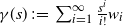 $\gamma(s) \, :\!= \, \sum_{i=1}^\infty {\frac{s^i}{i!}}w_i$
. For
 $f\in \mathbb{N}$
, the coefficient of
 $s^f$
of
 $\gamma^k(s)/k!$
is
 \[\sum_{\sum ik_i=f, \sum k_i=k}\dfrac{(w_i/i!)^{k_i}}{k!}\cdot\binom{k}{{k_1 k_2 k_3\cdots k_f}}=\dfrac{B_{f,k}(\boldsymbol{w})}{f!}.\]
Hence the coefficient of
 $s^f$
of
 \[\exp(\gamma(s))=\sum_{k=0}^\infty \gamma(s)^k/k!\]
is
 \[\sum_{k=1}^f{B_{f,k}(\boldsymbol{w})}/{f!}={B_f(1,\boldsymbol{w})}/{f!}.\]
Namely,
 \begin{equation}\exp\Biggl(\sum_{i=1}^\infty \dfrac{s^i}{i!}w_i\Biggr)=1+\sum_{f=1}^\infty \dfrac{s^f}{f!}B_f(1,\boldsymbol{w}).\end{equation}
Comparing it with (A.3), we have
 $h_f=B_f(1,\boldsymbol{w})$
,
 $ f\in\mathbb{N}$
. This argument completes bijective reparameterization between
 $(h_f)_{f\in\mathbb{N}}$
and
 $\boldsymbol{w}$
.
Let us note that
 \[G(s)^\lambda=\exp\Biggl(\sum_{i=1}^\infty \frac{s^i}{i!}\lambda w_i\Biggr)\]
determines
 $h(\,f;\ \lambda)$
in the proof of Theorem 2.1. Therefore, using (1.3), we have
 \begin{equation}h(\,f;\ \lambda)=B_f(\lambda,\boldsymbol{w}).\end{equation}
Proof of Theorem
2.3. We begin by proving the ‘if’ part. Since
 $B_0(\boldsymbol{w})\equiv 1$
irrespective of
 $\boldsymbol{w}$
, we consider the case of
 $n\in \mathbb{N}$
. By definition (1.3),
 \[B_n(\lambda,\boldsymbol{w})=\sum_{k=1}^{n-1} \lambda^k B_{n,k}(\boldsymbol{w})+\lambda^n B_{n,n}(\boldsymbol{w})=\sum_{k=1}^{n-1} \lambda^k B_{n,k}(\boldsymbol{w})+\lambda^n w_1^n.\]
Because
 $B_{n,k}(\boldsymbol{w})$
is a weighted sum of the
 $w_i$
with non-negative weights,
 $\sum_{k=1}^{n-1} \lambda^k B_{n,k}(\boldsymbol{w})\ge 0$
when
 $\boldsymbol{w}\in \Omega_1$
and
 $\lambda\in \mathbb{R}_{0+}$
. We observe that
 $\lambda^n w_1^n>0$
when
 $\lambda\in \mathbb{R}_+$
and
 $w_1\in \mathbb{R}_+$
. Therefore
 $B_n(\lambda,\boldsymbol{w})$
is strictly positive for
 $n\in\mathbb{N}_0$
when
 $\lambda\in \mathbb{R}_+$
and
 $\boldsymbol{w}\in \Omega_1$
. Consequently, (2.8) satisfies (2.4) for
 $n\in \mathbb{N}_0, J\in \mathbb{N}$
, and
 $\boldsymbol{\lambda}_J\in \mathbb{R}_+^J$
if
 $\boldsymbol{w}\in \Omega_1$
. When
 $\boldsymbol{w}\in \Omega_2$
, using (1.2) results in the same argument because
 $(\!-\!1)^{\sum_{j=1}^J{f_j}}=(\!-\!1)^n$
.
Next, the ‘only if’ part follows. If the sign of
 $\lim_{l\to +0}B_f(l,\boldsymbol{w})$
is different from that of
 $\lim_{l\to +\infty }B_f(l,\boldsymbol{w})$
, then there exists
 $\lambda\in\mathbb{R}_+$
such that
 $B_f(\lambda,\boldsymbol{w})=0$
since
 $B_f(l,\boldsymbol{w})$
is a continuous function of l. Therefore the condition of
 $p(\,\boldsymbol{f}_J)>0$
excludes
 $\boldsymbol{w}$
that satisfies
 \[\operatorname{sgn}\Bigl(\lim_{l\to +0}B_f(l,\boldsymbol{w})\Bigr)\neq\operatorname{sgn}\Bigl(\lim_{l\to +\infty }B_f(l,\boldsymbol{w})\Bigr).\]
By (1.4) and (1.5), we thus discard
 $\boldsymbol{w}$
such that
 $\operatorname{sgn}(l w_f)\neq\operatorname{sgn}(l^f w_1^f)$
for some
 $f\in \mathbb{N}_0$
. Accordingly,
 $\operatorname{sgn}(w_1)$
determines
 $\operatorname{sgn}(w_i)$
for all
 $i\ge 2$
. Hence either
 $\boldsymbol{w}\in \Omega_1$
or
 $\boldsymbol{w}\in \Omega_2$
is allowed when
 $\lambda_j\in \mathbb{R}_+$
. The case of
 $w_1=0$
is excluded because then
 $B_{1,1}(\boldsymbol{w})=0$
, which contradicts (2.4).
Proof of Theorem 2.8. Rewrite (2.12) as
 \[G(s)=\exp\Biggl(\sum_{i=1}^\infty \frac{s^i}{i!} (\lambda q_i\,i!)\Biggr)\exp(\!-\!\lambda).\]
Then, from (A.4),
 \[\exp(\lambda)G(s)=1+\sum_{f=1}^\infty \frac{s^f}{f!}B_f(\lambda,(q_i\,i!)_{i\in\mathbb{N}}).\]
Therefore
 \[\mathbb{P}(F_j=f)=\exp(\!-\!\lambda_j)B_f(\lambda_j,(q_i\,i!)_{i\in\mathbb{N}})/f!.\]
Also,
 \[\mathbb{P}\Biggl(\sum_{j=1}^JF_j=n\Biggr)=\exp(\!-\!\lambda_{\bullet})B_n(\lambda_{\bullet},(q_i\,i!)_{i\in\mathbb{N}})/n!,\]
since the PGF of
 $\sum_{j=1}^JF_j$
is
 \[\exp\Biggl(\lambda_{\bullet}\Biggl(\sum_{i=1}^\infty s^iq_i-1\Biggr)\Biggr).\]
Combining these results, the conditional distribution of
 $\boldsymbol{F}_J$
given
 $\sum_{j=1}^JF_j=n$
is
 \[\mathtt{BP}_{J}(n,\boldsymbol{\lambda}_{J};(q_i\,i!)_{i\in\mathbb{N}}).\]
Then
 $\mathbb{P}(\sum_{j=1}^JF_j=n)>0$
for all n is equivalent to
 $B_n(\lambda_{\bullet},(q_i\,i!)_{i\in\mathbb{N}})>0$
for all n. We have already proved in Theorem 2.3 that this positivity is equivalent to
 $(q_i\,i!)_{i\in\mathbb{N}}\in \Omega_1$
or
 $\boldsymbol{q}\in \Omega_1$
.
Proof of Theorem 3.3. First, write the score function as
 \begin{equation}\dfrac{\partial \log p(\boldsymbol{F}_J; \boldsymbol{\lambda}_J)}{\partial\lambda_j}=\dfrac{\partial B_{F_j}(\lambda_j,\boldsymbol{w})/\partial \lambda_j}{B_{F_j}(\lambda_j,\boldsymbol{w})}-\dfrac{\partial B_{n}(\lambda_{\bullet},\boldsymbol{w})/\partial \lambda_j}{B_{n}(\lambda_{\bullet},\boldsymbol{w})}.\end{equation}
The expectation of the score function is zero because
 \begin{align}\mathbb{E}\biggl[\dfrac{\partial B_{F_j}(\lambda_j,\boldsymbol{w})/\partial \lambda_j}{B_{F_j}(\lambda_j,\boldsymbol{w})}\biggr]& = \sum_{\boldsymbol{f}_J}\dfrac{n!}{B_n(\lambda_{\bullet}, \boldsymbol{w})}\prod_{i=1}^J\dfrac{B_{f_i}(\lambda_i,\boldsymbol{w})}{f_i!}\dfrac{\partial B_{f_j}(\lambda_j,\boldsymbol{w})/\partial \lambda_j}{B_{f_j}(\lambda_j,\boldsymbol{w})}\nonumber\\&= \dfrac{n!}{B_n(\lambda_{\bullet}, \boldsymbol{w})}\sum_{f_j=0}^n\dfrac{B_{n-f_j}(\lambda_{\bullet}-\lambda_j,\boldsymbol{w})\partial B_{f_j}(\lambda_j,\boldsymbol{w})/\partial \lambda_j}{(n-f_j)!\,f_j!}\nonumber\\&= \dfrac{n!}{B_n(\lambda_{\bullet}, \boldsymbol{w})}\dfrac{\partial}{\partial \lambda_j}\sum_{f_j=0}^n\dfrac{B_{n-f_j}(\lambda_{\bullet}-\lambda_j,\boldsymbol{w})B_{f_j}(\lambda_j,\boldsymbol{w})}{(n-f_j)!\,f_j!}\nonumber\\&=\dfrac{\partial B_{n}(\lambda_{\bullet},\boldsymbol{w})/\partial \lambda_j}{B_{n}(\lambda_{\bullet},\boldsymbol{w})}.\end{align}
Replacing
 $(\partial/\partial \lambda_j)$
with
 $(\partial^2/(\partial \lambda_j)^2)$
in (A.7), we also obtain
 \begin{equation}\mathbb{E}\biggl[\dfrac{\partial^2 B_{F_j}(\lambda_j,\boldsymbol{w})/(\partial \lambda_j)^2}{B_{F_j}(\lambda_j,\boldsymbol{w})}\biggr]=\dfrac{\partial^2 B_{n}(\lambda_{\bullet},\boldsymbol{w})/(\partial \lambda_j)^2}{B_{n}(\lambda_{\bullet},\boldsymbol{w})}.\end{equation}
Noting that
 \begin{equation}\dfrac{\partial}{\partial \lambda_j}\dfrac{\partial B_{F_j}(\lambda_j,\boldsymbol{w})/\partial \lambda_j}{B_{F_j}(\lambda_j,\boldsymbol{w})}=\dfrac{\partial^2 B_{F_j}(\lambda_j,\boldsymbol{w})/(\partial \lambda_j)^2}{B_{F_j}(\lambda_j,\boldsymbol{w})}-\biggl(\dfrac{\partial B_{F_j}(\lambda_j,\boldsymbol{w})/\partial \lambda_j}{B_{F_j}(\lambda_j,\boldsymbol{w})}\biggr)^2,\end{equation}
the differentiation of (A.6) yields
 \begin{align*}\dfrac{\partial^2 \log p(\boldsymbol{F}_J; \boldsymbol{\lambda}_J)}{(\partial \lambda_j)^2}& =\dfrac{\partial^2 B_{F_j}(\lambda_j,\boldsymbol{w})/(\partial \lambda_j)^2}{B_{F_j}(\lambda_j,\boldsymbol{w})}-\biggl(\dfrac{\partial B_{F_j}(\lambda_j,\boldsymbol{w})/\partial \lambda_j}{B_{F_j}(\lambda_j,\boldsymbol{w})}\biggr)^2\\& \quad -\dfrac{\partial^2 B_{n}(\lambda_{\bullet},\boldsymbol{w})/(\partial \lambda_j)^2}{B_{n}(\lambda_{\bullet},\boldsymbol{w})}+\biggl(\dfrac{\partial B_{n}(\lambda_{\bullet},\boldsymbol{w})/\partial \lambda_j}{B_{n}(\lambda_{\bullet},\boldsymbol{w})}\biggr)^2.\end{align*}
Then taking expectation on both sides results in (3.2) because of (A.8).
Next, (3.2) equals
 \[\mathbb{E}\biggl[\dfrac{\partial^2 B_{F_j}(\lambda_j,\boldsymbol{w})/(\partial \lambda_j)^2}{B_{F_j}(\lambda_j,\boldsymbol{w})}\biggr]-\mathbb{E}\biggl[\dfrac{\partial}{\partial \lambda_j}\biggl(\dfrac{\partial B_{F_j}(\lambda_j,\boldsymbol{w})/\partial \lambda_j}{B_{F_j}(\lambda_j,\boldsymbol{w})}\biggr)\biggr]-\biggl(\dfrac{\partial B_{n}(\lambda_{\bullet},\boldsymbol{w})/\partial \lambda_j}{B_{n}(\lambda_{\bullet},\boldsymbol{w})}\biggr)^2\]
because of (A.9). This expression reduces to (3.3) by (A.8). Therefore the diagonal elements have been shown to be (3.2) or (3.3).
Next we differentiate (A.6) as
 \[\frac{\partial^2 \log p(\boldsymbol{F}_J; \boldsymbol{\lambda}_J)}{\partial \lambda_i\partial\lambda_j} =-\frac{\partial}{\partial \lambda_i}\frac{\partial B_{n}(\lambda_{\bullet},\boldsymbol{w})/\partial \lambda_j}{B_{n}(\lambda_{\bullet},\boldsymbol{w})},\]
which equals
 \[-\frac{\partial^2 B_{n}(\lambda_{\bullet},\boldsymbol{w})/(\partial \lambda_i\partial \lambda_j)}{B_n(\lambda_{\bullet},\boldsymbol{w})}+\frac{(\partial B_{n}(\lambda_{\bullet},\boldsymbol{w})/\partial \lambda_i)(\partial B_{n}(\lambda_{\bullet},\boldsymbol{w})/\partial \lambda_j)}{B_n(\lambda_{\bullet},\boldsymbol{w})^2}.\]
Then taking expectation on both sides produces (3.4).
Proof of Theorem
3.4. Without loss of generality, we consider the two-dimensional case that
 $(F_1,F_2)\sim\mathtt{BP}_2(n,\lambda_1,\lambda_2;\,\boldsymbol{w})$
, and the moments of
 $F_1$
are shown.
Define
 \[\eta(s) \, :\!= \, \sum_{i=0}^\infty \frac{s^i}{i!}w_i.\]
Then
 \[G(s)=\sum_{i=0}^\infty \exp(w_0\lambda_{\bullet})\frac{B_i(\lambda_{\bullet},\boldsymbol{w})}{i!}s^i=\exp(\lambda_{\bullet}\eta(s)).\]
We denote
 $G_1(s)=\exp(\lambda_1\eta(s))$
and
 $G_2(s)=\exp(\lambda_2\eta(s))$
. Write
 $\mathrm{d}G_1(s)/\mathrm{d}s$
as
 \[G_1'(s)=\sum_{i=0}^\infty \exp(w_0\lambda_1)\frac{B_i(\lambda_1,\boldsymbol{w})}{(i-1)!}s^{i-1}=G_1(s)\lambda_1\eta'(s),\]
where
 $\eta'(s)=\mathrm{d}\eta(s)/\mathrm{d}s$
. Then
 \begin{equation}G_1'(s)G_2(s)=\exp(w_0(\lambda_1+\lambda_2))\sum_{n=0}^\infty \sum_{i=0}^n\dfrac{iB_i(\lambda_1,\boldsymbol{w})B_{n-i}(\lambda_2,\boldsymbol{w})}{i!\,(n-i)!}s^{n-1}.\end{equation}
Also, since
 \[\mathrm{d}G(s)/\mathrm{d}s=G'(s)=G(s)(\lambda_1+\lambda_2)\mathrm{d}\eta(s)/\mathrm{d}s,\]
we obtain
 \[\frac{\lambda_1}{\lambda_1+\lambda_2}G'(s)=\lambda_1G(s)\mathrm{d}\eta(s)/\mathrm{d}s=G_1'(s)G_2(s),\]
using
 $G(s)=G_1(s)G_2(s)$
. Then we equate the coefficient of
 $s^{n-1}$
between (A.10) and
 \[\frac{\lambda_1}{\lambda_1+\lambda_2}G'(s)=\frac{\lambda_1}{\lambda_1+\lambda_2}\sum_{n=0}^\infty \exp(w_0(\lambda_1+\lambda_2))\frac{B_n((\lambda_1+\lambda_2),\boldsymbol{w})}{(n-1)!}s^{n-1}.\]
It follows that
 \[\sum_{i=0}^n\frac{iB_i(\lambda_1,\boldsymbol{w})B_{n-i}(\lambda_2,\boldsymbol{w})}{i!\,(n-i)!}=\frac{B_n((\lambda_1+\lambda_2),\boldsymbol{w})}{n!}\frac{n\lambda_1}{\lambda_1+\lambda_2}.\]
Dividing both sides by
 $B_n((\lambda_1+\lambda_2),\boldsymbol{w})/n!$
, we obtain
 $\mathbb{E}(F_1)=n\lambda_1/(\lambda_1+\lambda_2)$
, which shows (3.5).
On the variance, we use the second derivative:
 \[G_1''(s) = \lambda_1\{G_1'(s)\eta'(s)+G_1(s)\eta''(s)\}= \lambda_1^2 G_1(s)\eta'(s)\eta'(s)+\lambda_1G_1(s)\eta''(s).\]
Hence
 \[G_1''(s)G_2(s)=\lambda_1^2 G(s)\eta'(s)\eta'(s)+\lambda_1G(s)\eta''(s).\]
By
 $G(s)\eta'(s)=G'(s)/(\lambda_1+\lambda_2)$
,
 \begin{align*}G_1''(s)G_2(s) &= \dfrac{\lambda_1^2}{\lambda_1+\lambda_2}\biggl\{G'(s)\eta'(s)+\dfrac{\lambda_1+\lambda_2}{\lambda_1}G(s)\eta''(s)\biggr\}\\&= \dfrac{\lambda_1^2}{\lambda_1+\lambda_2}\biggl\{\dfrac{G''(s)}{\lambda_1+\lambda_2}+\dfrac{\lambda_2}{\lambda_1}G(s)\eta''(s)\biggr\}\\&= \biggl(\dfrac{\lambda_1}{\lambda_1+\lambda_2}\biggr)^2G''(s)+\dfrac{\lambda_1\lambda_2}{\lambda_1+\lambda_2}G(s)\eta''(s).\end{align*}
Then, noting that
 \[G(s)\eta''(s) = \sum_{i=0}^\infty \mathrm{e}^{w_0(\lambda_1+\lambda_2)}\frac{B_i((\lambda_1+\lambda_2),\boldsymbol{w})}{i!}s^i\times \sum_{i=0}^\infty \frac{w_i}{i!}i(i-1)s^{i-2},\]
which equals
 \[\sum_{n=0}^\infty \sum_{i=0}^n\mathrm{e}^{w_0(\lambda_1+\lambda_2)}\frac{B_i((\lambda_1+\lambda_2),\boldsymbol{w})}{i!}\frac{w_{n-i}}{(n-i)!}(n-i)(n-i-1)s^{n-2},\]
we obtain
 \begin{align}& {G_1''(s)G_2(s)}\nonumber\\ &\quad =\biggl(\dfrac{\lambda_1}{\lambda_1+\lambda_2}\biggr)^2\sum_{i=0}^\infty \mathrm{e}^{w_0(\lambda_1+\lambda_2)}\dfrac{i(i-1)B_i((\lambda_1+\lambda_2),\boldsymbol{w})}{i!}s^{i-2}\nonumber\\& \quad \quad +\dfrac{\lambda_1\lambda_2}{\lambda_1+\lambda_2}\sum_{n=0}^\infty \sum_{i=0}^n\mathrm{e}^{w_0(\lambda_1+\lambda_2)}\dfrac{B_i((\lambda_1+\lambda_2),\boldsymbol{w})}{i!}w_{n-i}(n-i)(n-i-1)s^{n-2}.\end{align}
Alternatively,
 \begin{align}G_1''(s)G_2(s) & = \mathrm{e}^{w_0(\lambda_1+\lambda_2)}\sum_{n=0}^\infty \sum_{i=0}^n\dfrac{i(i-1)B_i(\lambda_1,\boldsymbol{w})B_{n-i}(\lambda_2,\boldsymbol{w})}{i!\,(n-i)!}s^{n-2}\nonumber\\&= \mathrm{e}^{w_0(\lambda_1+\lambda_2)}\sum_{n=0}^\infty \mathbb{E}(F_1(F_1-1))\dfrac{B_n((\lambda_1+\lambda_2),\boldsymbol{w})}{n!}s^{n-2}.\end{align}
Therefore, equating the coefficient of
 $s^{n-2}$
between (A.11) and (A.12), we have
 \[\mathbb{E}(F_1(F_1-1)) = \biggl(\frac{\lambda_1}{\lambda_1+\lambda_2}\biggr)^2n(n-1)+\frac{\lambda_1\lambda_2}{\lambda_1+\lambda_2}\frac{n!}{B_n((\lambda_1+\lambda_2),\boldsymbol{w})}\sum_{i=0}^n\frac{B_i((\lambda_1+\lambda_2),\boldsymbol{w})w_{n-i}}{i!\,(n-i-2)!}.\]
Since
 $\operatorname{Var}(F_1)=\mathbb{E}(F_1(F_1-1))+\mathbb{E}(F_1)-\mathbb{E}(F_1)^2$
, the variance (3.6) follows immediately.
On the covariance, we use
 $\operatorname{Var}(F_i+F_j)=\operatorname{Var}(F_i)+\operatorname{Var}(F_j)+2\operatorname{Cov}(F_i,F_j)$
. Because of the closure property of marginal variables,
 \[\operatorname{Var}(F_i+F_j)=n(\pi_i+\pi_j)(1-(\pi_i+\pi_j))\phi(n,\lambda_{\bullet},\boldsymbol{w}).\]
Then we have (3.7).
Proof of Theorem
3.5. For
 $n\in\mathbb{N}$
,
 \[B_n(\lambda,\boldsymbol{w})=\sum_{i=0}^{n-1}\binom{n-1}{i}B_i(\lambda,\boldsymbol{w})\lambda w_{n-i};\ \]
see e.g. [Reference Charalambides8, eq. 11.10]. It implies for
 $n\ge 2$
that
 \begin{equation}B_n(\lambda_{\bullet},\boldsymbol{w})-{B_{n-1}(\lambda_{\bullet},\boldsymbol{w}) \lambda_{\bullet} w_{1}}= \lambda_{\bullet}(n-1)!\,\sum_{i=0}^{n-2}\dfrac{B_i(\lambda_{\bullet},\boldsymbol{w}) w_{n-i}}{i!\,(n-i-1)!}.\end{equation}
Because
 $B_n(\lambda_{\bullet},\boldsymbol{w})>0$
in the parameter space, we divide the both sides of (A.13) by
 $B_n(\lambda_{\bullet},\boldsymbol{w})$
. Consequently,
 \begin{equation}1-\dfrac{B_{n-1}(\lambda_{\bullet},\boldsymbol{w}) \lambda_{\bullet} w_{1}}{B_n(\lambda_{\bullet},\boldsymbol{w}) }= \dfrac{\lambda_{\bullet}(n-1)!}{B_n(\lambda_{\bullet},\boldsymbol{w}) }\sum_{i=0}^{n-2}\dfrac{B_i(\lambda_{\bullet},\boldsymbol{w}) w_{n-i}}{i!\,(n-i-1)!}.\end{equation}
Therefore, for
 $n\ge 2$
,
 \[1-\frac{B_{n-1}(\lambda_{\bullet},\boldsymbol{w}) \lambda_{\bullet} w_{1}}{B_n(\lambda_{\bullet},\boldsymbol{w}) }\leq \frac{\lambda_{\bullet}(n-1)!}{B_n(\lambda_{\bullet},\boldsymbol{w})}\sum_{i=0}^{n-2}\frac{B_i(\lambda_{\bullet},\boldsymbol{w}) w_{n-i}}{i!\,(n-i-2)!}= \phi(n,\lambda_{\bullet},\boldsymbol{w})-1.\]
Hence the first inequality of (3.8) holds.
The middle term of (3.8) takes its minimum when (A.14) is minimized, where
 $w_i=0, i\ge 2$
, since all other elements of (A.14) are positive. Then the middle term of (3.8) equals one.
The following proof of (3.9) parallels that of (3.8).
Because of (A.13), it follows for
 $n\ge 2$
that
 \begin{align*}(n-1)\{B_n(\lambda_{\bullet},\boldsymbol{w})-{B_{n-1}(\lambda_{\bullet},\boldsymbol{w}) \lambda_{\bullet} w_{1}}\} & \ge\lambda_{\bullet}(n-1)!\,\sum_{i=0}^{n-2}\frac{B_i(\lambda_{\bullet},\boldsymbol{w})w_{n-i}}{i!\,(n-i-2)!}\\&= {B_n(\lambda_{\bullet},\boldsymbol{w})}(\phi(n,\lambda_{\bullet},\boldsymbol{w})-1).\end{align*}
Because
 $B_n(\lambda_{\bullet},\boldsymbol{w})>0$
in the parameter space, we divide the both sides of the above inequality by
 $B_n(\lambda_{\bullet},\boldsymbol{w})$
. Consequently,
 \[(n-1)(1-B_{n-1}(\lambda_{\bullet},\boldsymbol{w})\lambda_{\bullet} w_1/B_n(\lambda_{\bullet},\boldsymbol{w}))\ge \phi(n,\lambda_{\bullet},\boldsymbol{w})-1\quad \text{for $n\ge 2$.}\]
Hence the first inequality of (3.9) holds.
We observe in the parameter space that
 ${B_{n-1}(\lambda_{\bullet},\boldsymbol{w})\lambda_{\bullet} w_1}/ {B_n(\lambda_{\bullet},\boldsymbol{w})}>0$
. Therefore the middle term of (3.9) is strictly smaller than n.
As
 $\lambda_{\bullet}\to \infty $
,
 \[\phi(n,\lambda_{\bullet},\boldsymbol{w})-1=\frac{\lambda_{\bullet}(n-1)!}{\lambda_{\bullet}^n w_1^n+\boldsymbol{\mathrm{O}} (\lambda_{\bullet}^{n-1})}\biggl\{\frac{B_{n-2}(\lambda_{\bullet},\boldsymbol{w})w_{2}}{(n-2)!}+\boldsymbol{\mathrm{O}} (\lambda_{\bullet}^{n-3})\biggr\}= \boldsymbol{\mathrm{O}} (\lambda_{\bullet}^{-1})\]
due to (1.5). Therefore (3.10) holds.
As
 $\lambda_{\bullet}\to 0$
,
 \[\phi(n,\lambda_{\bullet},\boldsymbol{w})-1=\frac{\lambda_{\bullet}(n-1)!}{{\lambda_{\bullet}}{w_n}+\boldsymbol{\mathrm{O}} (\lambda_{\bullet}^{2})}\biggl\{\frac{B_{0}(\lambda_{\bullet},\boldsymbol{w})w_{n}}{(n-2)!}+\boldsymbol{\mathrm{O}} ({\lambda_{\bullet}})\biggr\}=(n-1)+\boldsymbol{\mathrm{O}} (\lambda_{\bullet})\]
Proof of Lemma
4.1. Generally,
 $\mathbb{E}(F_j)=\mathbb{E}_\pi(\mathbb{E}(F_j| \boldsymbol{\pi}_J))$
, where
 $\mathbb{E}_\pi(\! \cdot \!)$
implies that the expectation is taken under random
 $\boldsymbol{\pi}_J$
. Similarly,
 \[\operatorname{Var}(F_j)=\mathbb{E}_\pi({\kern-1.2pt}\operatorname{Var}(F_j\mid \boldsymbol{\pi}_J))+\operatorname{Var}_\pi(\mathbb{E}(F_j\mid \boldsymbol{\pi}_J))\]
and
 \[\operatorname{Cov}(F_i,F_j)=\mathbb{E}_\pi({\kern-1.5pt}\operatorname{Cov}(F_i,F_j\mid \boldsymbol{\pi}_J))+\operatorname{Cov}_\pi(\mathbb{E}(F_i\mid \boldsymbol{\pi}_J),\mathbb{E}(F_j\mid \boldsymbol{\pi}_J)).\]
The conditional moments of
 $F_j$
given
 $\boldsymbol{\pi}_J$
are provided in Theorem 3.4. Using these and taking the expectation under random
 $\boldsymbol{\pi}_J$
, the formulae are obtained.
Proof of Theorem 4.3. Write
 \[G(u)=\exp(\!-\!\mu_{\bullet}\psi(u))=\mathbb{E}(\mathrm{e}^{-uX_{\bullet}}).\]
Denote
 ${\mathrm d}G(u)/{\mathrm d}u$
by G’(u), and other derivatives are similarly denoted.
Because
 $\mathbb{P}(X_{\bullet}=0)=0$
is assumed,
 $G(\infty )=0$
and
 $G(0)=1$
. Also
 \[uG'(u)=u\frac{\mathrm d}{\mathrm{d}u}\int_0^\infty \mathrm{e}^{-ut}F_{X_{\bullet}}(\mathrm{d}t)=u\int_0^\infty \frac{\mathrm{d}\mathrm{e}^{-ut}}{\mathrm{d}u}F_{X_{\bullet}}(\mathrm{d}t)=\mathbb{E}\biggl(-\frac{uX_{\bullet}}{\mathrm{e}^{uX_{\bullet}}}\biggr),\]
which implies that
 \begin{equation}[uG'(u)]_0^\infty =0.\end{equation}
Proposition 2 of [Reference Favaro, Hadjicharalambous and Prünster21] implies that
 \[\mathbb{E}({P_j})=\int_{0}^\infty \mu_j\psi'(u)\exp(\!-\!\mu_{\bullet}\psi(u))\,\mathrm{d}u.\]
Noting that
 $\psi'(u)\exp(\!-\!\mu_{\bullet}\psi(u))=G'(u)/(\!-\!\mu_{\bullet})$
, we have
 \[\mathbb{E}({P_j})=-\rho_j\int_{0}^\infty G'(u)\,\mathrm{d}u=-\rho_j[G(u)]_0^\infty =\rho_j.\]
Hence (4.6) is proved.
Equation (7) of [Reference Favaro, Hadjicharalambous and Prünster21] implies that
 \begin{equation}\mathbb{E}(P_j^2)=\int_{0}^\infty u\biggl(\dfrac{\mathrm{d}^2\exp(\!-\!\mu_j\psi(u))}{\mathrm{d}u^2}\biggr)\exp(-(\mu_{\bullet}-\mu_{j})\psi(u))\,\mathrm{d}u.\end{equation}
Then, by
 \[({\mathrm{d}^2}/{\mathrm{d}u^2})\exp(\!-\!\mu\psi(u))=(\!-\!\mu)\psi''(u)\exp(\!-\!\mu\psi(u))+\mu^2(\psi'(u))^2\exp(\!-\!\mu\psi(u)),\]
(A.16) can be rewritten as
 \begin{align*}\mathbb{E}(P_j^2) &= \int_{0}^\infty u\{(\!-\!\mu_j)\psi''(u)G(u)+{\mu_j}^2(\psi'(u))^2G(u)\}\,\mathrm{d}u\\&=\int_{0}^\infty u\{(\!-\!\mu_j)\psi''(u)G(u)+{\mu_j}^2\psi'(u)G'(u)/(\!-\!\mu_{\bullet})\}\,\mathrm{d}u\end{align*}
since
 $\psi'(u)G(u)=G'(u)/(\!-\!\mu_{\bullet})$
. Further,
 $\psi'(u)G'(u)=G''(u)/(\!-\!\mu_{\bullet})-\psi''(u)G(u)$
, and thus
 \begin{align*}\mathbb{E}(P_j^2) &= \int_{0}^\infty u\{({\mu_j}^2/\mu_{\bullet}-\mu_j)\psi''(u)G(u)+(\mu_j/\mu_{\bullet})^2G''(u)\}\,\mathrm{d}u\\&= \int_{0}^\infty \{\lambda_{\bullet}\rho_j(\rho_j-1)u\psi''(u)G(u)+\pi_j^2uG''(u)\}\,\mathrm{d}u.\end{align*}
Employing integration by parts,
 \begin{equation}\int_0^\infty uG''(u)\,\mathrm{d}u=[uG'(u)]^\infty _0-\int_0^\infty G'(u)\,\mathrm{d}u=1\end{equation}
because of (A.15). Hence
 \[\mathbb{E}(P_j^2)= \rho_j(1-\rho_j)(\!-\!\mu_{\bullet})\int_{0}^\infty u\psi''(u)G(u)\,\mathrm{d}u+\rho_j^2.\]
Because
 $\operatorname{Var}(P_j)=\mathbb{E}(P_j^2)-\mathbb{E}(P_j)^2$
,
 \begin{equation}\varphi(\mu_{\bullet})=-\mu_{\bullet} \int_{0}^\infty u\psi''(u)G(u)\,\mathrm{d}u.\end{equation}
Then, by
 \[\psi''(u)G(u)=G''(u)/(\!-\!\mu_{\bullet})-\psi'(u)G'(u)=G''(u)/(\!-\!\mu_{\bullet})+\mu_{\bullet}(\psi'(u))^2G(u),\]
we have
 \begin{equation}\varphi(\mu_{\bullet})=\int_{0}^\infty uG''(u)\,\mathrm{d}u-\mu_{\bullet}^2\int_{0}^\infty u(\psi'(u))^2G(u)\,\mathrm{d}u.\end{equation}
The first term of the right-hand side of (A.19) is unity because of (A.17), which shows (4.7).
The covariance (4.8) can be shown by noting that
 \[\operatorname{Var}(P_i+P_j)=(\pi_i+\pi_j)(1-(\pi_i+\pi_j))\eta(\lambda_{\bullet})=\operatorname{Var}(P_i)+\operatorname{Var}(P_j)+2\operatorname{Cov}(P_i,P_j);\ \]
the first equation holds because
 $\mathbb{E}(\mathrm{e}^{-u(X_i+X_j)})=\exp(\!-\!(\mu_i+\mu_j)\psi(u))$
.
Two lemmas for Theorem 4.5
Lemma A.1. Let
 $\nu$
be a Lévy measure, and
 $\mu\in \mathbb{R}_+$
. Write the Laplace transform of an
 $\mathbb{R}_+$
-valued random variable M as
 $\exp(\!-\!\mu\psi(u))$
, where
 $\psi(u)=\int (1-\mathrm{e}^{-ux})\nu(\mathrm{d}x)$
. Then a random variable satisfies
 $F\sim \mathtt{Po}(M)$
if and only if
 $\mathbb{E}(s^{F})=\exp(\!-\!\mu \psi(1-s))$
.
Proof of Lemma A.1. This link between the PGF of a mixed Poisson distribution and the Laplace transform of its mixing distribution is widely known; see [Reference Grandell26, Proposition 2.1(vi)].
Lemma A.2. In Lemma A.1,
 \[\mathbb{P}(F=f)=\exp(\!-\!\mu\psi(1))B_f(\mu,\boldsymbol{w})/f!,\]
where
 $\boldsymbol{w}$
satisfies (4.11).
Proof of Lemma
A.2.Because
 $\mathbb{E}(s^{F})=\sum_{f=0}^\infty \mathbb{P}(F=f)s^f$
, we obtain
 $\mathbb{P}(F=f)$
by differentiating
 $\exp(\!-\!\mu \psi(1-s))$
. First, expand
 \[-\psi(1-s)=\sum_{i=0}^\infty \frac{s^i}{i!}w_i.\]
Then
 $w_0=-\psi(1)$
, and
 $\boldsymbol{w}$
satisfies (4.11). Let
 \[G(s)=\exp\Biggl(\sum_{i=0}^\infty \frac{s^i}{i!}w_i\Biggr)=\sum_{f=0}^\infty \frac{s^f}{f!}h_f.\]
By (A.4),
 $h_f=\exp(w_0)B_f(\boldsymbol{w})$
. Noting that
 $\mathbb{E}(s^{F})=G(s)^\mu$
, we obtain
 $\mathbb{P}(F=f)$
.
Proof of Theorem
4.5. Suppose that
 $F_j\sim \mathtt{Po}(M_j)$
,
 $j\in[J]$
, independently, where the Laplace transform of
 $M_j$
is
 $\exp(\!-\!\mu_j\psi(u))$
. Write
 \[\boldsymbol{M}_J \, :\!= \, (M_1,M_2,\ldots,M_J)\quad \text{and}\quad \boldsymbol{m}_J \, :\!= \, (m_1,m_2,\ldots,m_J).\]
Then
 \[\mathbb{P}\Biggl(\boldsymbol{F}_J=\boldsymbol{f}_J\biggm|\sum_{j=1}^JF_j=n,\boldsymbol{M}_J=\boldsymbol{m}_J\Biggr)=\binom{n}{\boldsymbol{f}_J}\prod_{j=1}^J\biggl(\frac{m_j}{m_{\bullet}}\biggr)^{f_j}.\]
Taking the expectation over
 $\boldsymbol{M}_J$
,
 \[\mathbb{P}\Biggl(\boldsymbol{F}_J=\boldsymbol{f}_J\biggm|\sum_{j=1}^Jf_j=n\Biggr)=\int_{\mathbb{R}_+^J} \binom{n}{\boldsymbol{f}_J}\prod_{j=1}^J\biggl(\frac{m_j}{m_{\bullet}}\biggr)^{f_j}\,\mathrm{d}F(\boldsymbol{m}_J).\]
Next we transform variables so that
 $p_j=m_j/m_{\bullet}$
,
 $j\in[J]$
, and integrate out
 $m_{\bullet}$
. Write
 $\boldsymbol{p}_{J-1} \, :\!= \, (p_1,p_2,\ldots,p_{J-1})$
, and the Jacobian of
 $\boldsymbol{m}_J\mapsto (\boldsymbol{p}_{J-1},m_{\bullet})$
is
 $m_{\bullet}^{J-1}$
. Therefore
 \begin{align}{\mathbb{P}\Biggl(\boldsymbol{F}_J=\boldsymbol{f}_J\biggm|\sum_{j=1}^JF_j=n\Biggr)}&= \int_{\triangle^{J-1}\times \mathbb{R}_+} \binom{n}{\boldsymbol{f}_J}\prod_{j=1}^Jp_j^{f_j}m_{\bullet}^{J-1}\,\mathrm{d}F(\boldsymbol{p}_{J-1},m_{\bullet})\nonumber\\&= \int_{\triangle^{J-1}}\binom{n}{\boldsymbol{f}_J}\prod_{j=1}^Jp_j^{f_j}\,\mathrm{d}F(\boldsymbol{p}_{J-1}).\end{align}
The right-hand side of (A.20) equals
 $\mathtt{Mn}(n,\boldsymbol{\pi}_J)\mathop{\land}_{\boldsymbol{\pi}_J}\mathtt{NID}_J(\boldsymbol{\mu}_J\times\nu)$
. On the other hand, each
 \[\mathbb{P}(F_j=f_j)=\exp(\!-\!\mu_j\psi(1))B_{f_j}(\mu_j,\boldsymbol{w})/f_j!\]
by Lemma A.2. Then, similarly to Theorem 2.8, the left-hand side of (A.20) equals the PMF of
 $\mathtt{BP}_J(n,\boldsymbol{\mu}_J;\,\boldsymbol{w})$
. Hence (4.12) holds.
Proof of Theorem
4.6. By Theorem 4.5, if
 $\boldsymbol{w}$
satisfies (4.11) of a proper distribution
 $\nu$
, then the PGF of
 $(F_{1,n},F_{2,n},\ldots,F_{J,n})$
equals that of
 $\mathtt{Mn}_J(n,\boldsymbol{\pi}_J)\mathop{\land}_{\boldsymbol{\pi}_J}\mathtt{NID}_{J}(\boldsymbol{\mu}_J\times\nu)$
for all
 $n\in\mathbb{N}$
. If so,
 \[(F_{1,n},F_{2,n},\ldots,F_{J,n}\mid \boldsymbol{\pi}_J)\sim\mathtt{Mn}_J(n,\boldsymbol{\pi}_J).\]
Then the multivariate Lindeberg–Lévy central limit theorem applies, and
 \[(F_{1,n}/n,F_{2,n}/n,\ldots,F_{J,n}/n\mid \boldsymbol{\pi}_J)\stackrel{\boldsymbol{p}}{\to}\boldsymbol{\pi}_J\quad \text{as $n\to \infty $;}\]
see [Reference Serfling48, Theorem 2.7 (p. 109) and Application C (p. 26)]. Therefore the conditional PGF of
 $(F_{1,n}/n,F_{2,n}/n,\ldots,F_{J,n}/n)$
given
 $\boldsymbol{\pi}_J$
converges as
 $n\to \infty $
:
 \[\mathbb{E}\Biggl(\prod_{j=1}^Jz_j^{F_{j,n}/n}\mid \boldsymbol{\pi}_J\Biggr)\to\prod_{j=1}^Jz_j^{\pi_j}.\]
Hence the PGF of
 $(F_{1,n}/n,F_{2,n}/n,\ldots,F_{J,n}/n)$
unconditionally converges to
 $\mathbb{E}_{\boldsymbol{\pi}_J}(\prod_{j=1}^Jz_j^{\pi_j})$
, which is the PGF of
 $\mathtt{NID}_{J}(\boldsymbol{\mu}_J\times\nu)$
.
Proof of Theorem
4.8. Suppose that
 $\boldsymbol{v}=(1,0,0,\ldots)$
in Theorem 4.7. Then we obtain
 $\boldsymbol{F}_J\sim\mathtt{BP}_J(n,\boldsymbol{\mu}_J;\,\boldsymbol{w})$
by Theorem 4.5. The marginal variance of this distribution is given by (3.6). This expression has to equal the special case of the variance formula of Theorem 4.7 with
 $\phi(n,\lambda_{\bullet},\boldsymbol{v})=1$
. Hence (4.13) holds.
Direct proof of Proposition 5.1. By induction, it holds that
 \begin{align*} \sum_{i=0}^n{\Gamma(\alpha+i)}/{\Gamma(1+i)}={\Gamma(1+n+\alpha)}/{a\Gamma(1+n)}. \end{align*}
Using this equation, we have
 \begin{align*} \frac{(n-1)!\,\alpha}{\Gamma(\alpha+n)}\sum_{i=0}^{n-2}\frac{(n-i-1)\Gamma(\alpha+i)}{\Gamma(i+1)}&= \frac{(n-1)!\,\alpha}{\Gamma(\alpha+n)}\Biggl\{(n-1)\sum_{i=0}^{n-2}\frac{\Gamma(\alpha+i)}{\Gamma(i+1)}-\sum_{i=1}^{n-2}\frac{\Gamma(\alpha+i)}{\Gamma(i)}\Biggr\}\\&= \frac{(n-1)!\,\alpha}{\Gamma(\alpha+n)}\biggl\{(n-1)\frac{\Gamma(n-1+\alpha)}{\alpha\Gamma(n-1)}-\frac{\Gamma(n-1+\alpha)}{(\alpha+1)\Gamma(n-2)}\biggr\}\\&= \frac{(n-1)!\,\alpha}{\Gamma(\alpha+n)}\biggl\{\frac{\Gamma(n+\alpha)}{\alpha(\alpha+1)\Gamma(n-1)}\biggr\}\\&= \frac{n-1}{\alpha+1}.\\[-36pt] \end{align*}
Proof of Theorem
6.1. Corollary 2.20 of [Reference Breiman6] states conditions of such
 $\boldsymbol{F}$
to exist, which are confirmed below: it is apparent that
 $p_t(\! \cdot \!)\ge 0$
and
 $\sum_{f_1}p_2(\,f_1,n-f_1)=1$
. The key condition is that
 \[\sum_{f_{t}}p_{t+1}\Biggl(\,\boldsymbol{f}_{t},n-\sum_{j=1}^{t}f_j\Biggr)=p_t\Biggl(\,\boldsymbol{f}_{t-1},n-\sum_{j=1}^{t-1}f_j\Biggr).\]
This equation holds because Theorem 3.1 ensures that
 \[\Biggl(\boldsymbol{F}_{t-1},n-\sum_{j=1}^{t-1}F_j\Biggr)\sim\mathtt{BP}_t\Biggl(n,\Biggl(\boldsymbol{\lambda}_{t-1},\lambda_{\bullet}-\sum_{j=1}^{t-1}\lambda_j\Biggr);\,\boldsymbol{w}\Biggr)\]
when
 \[\Biggl(\boldsymbol{F}_{t},n-\sum_{j=1}^t F_j\Biggr)\sim\mathtt{BP}_{t+1}\Biggl(n,\Biggl(\boldsymbol{\lambda}_t,\lambda_{\bullet}-\sum_{j=1}^t\lambda_j\Biggr);\,\boldsymbol{w}\Biggr).\]
These conditions hold within the parameter space of the BPD.
Proof of Theorem
6.3. The PGF of
 $\boldsymbol{S}_{n,J}$
is expressed as
 \[\mathbb{E}\Biggl(\prod_{i=1}^nz_i^{S_{i,J}}\Biggr) = \prod_{j=1}^J\Biggl\{1+\sum_{i=1}^n\frac{z_i}{i!}\sum_{k=1}^i{\lambda_{j,J}}^kB_{i,k}(\boldsymbol{w})\Biggr\}\frac{n!}{B_n(\lambda_{\bullet},\boldsymbol{w})}.\]
Then the assumption that
 $\lambda_{j,J}=\mu/J+\boldsymbol{\mathrm{o}} (J^{-1})$
lets the right-hand side be
 \[\Biggl\{1+\sum_{i=1}^n\frac{z_i}{i!}\biggl(\frac{\mu w_i}{J}+\boldsymbol{\mathrm{o}} (J^{-1})\biggr)\Biggr\}^J\frac{n!}{B_n(\lambda_{\bullet},\boldsymbol{w})}\to \exp\Biggl(\mu\sum_{i=1}^n\frac{z_i}{i!}w_i\Biggr)\frac{n!}{B_n(\mu,\boldsymbol{w})}\quad \text{as $J\to \infty $.}\]
The last expression is the PGF of (6.3).



