2. Tetrad magneto-hydrodynamics

The tetrad formalism was developed in the framework of HD. This formalism makes use of Lagrangian variables describing the fluid as a collection of ‘macroscopically infinitesimal’ parcels (Materassi Reference Materassi and Schulz2014, Reference Materassi2015). Its introduction was motivated by the need for extending to finite size observation and simulations, the results regarding ‘local topology’ of the fields in Viellefosse (Reference Vieillefosse1984) and Cantwell (Reference Cantwell1992). As discussed below, the necessity for encoding the effects of scales smaller than the one considered, and of the nearby parcels, yields the introduction of stochastic forces in the equations. This implies the necessity for introducing a stochastic formalism. The physical properties of fluctuations, described in terms of spectrum and correlations, are encoded in the assumptions made about these noise terms.

The parcels are so small that their size may be considered as infinitesimal within a Taylor approximation of fields in a laminar regime, although they are still macroscopic objects to contain enough particles to have proper thermodynamics (Rai Choudhuri Reference Rai Choudhuri1998; Bennett Reference Bennett2006). Outside laminar regimes, in the presence of turbulence, considerations of the smallness of high-order terms in such expansions must be viewed in terms of ensemble averages, as explained in the following analysis.

Figure 1.

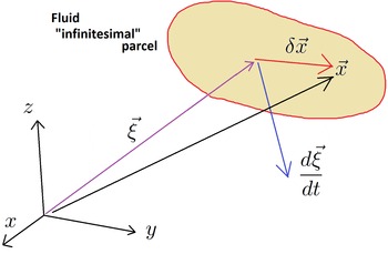
The points $\boldsymbol{x}$ in the parcel and the centre-of-mass ${\bf\xi}$ of the parcel, as in (2.1). The speed $\text{d}{\bf\xi}/\text{d}t$ represents the collective motion of the parcel, see Materassi (Reference Materassi and Schulz2014, Reference Materassi2015).

Consider a similar small volume of continuum matter. If ${\bf\xi}$ is its centre-of-mass, a smooth field ${\it\varphi}$ at a point $\boldsymbol{x}$ still within the parcel, so that $\boldsymbol{x}={\bf\xi}+{\it\delta}\boldsymbol{x}$ (see figure 1) is approximated as ${\it\varphi}(\boldsymbol{x})={\it\varphi}({\bf\xi})+{\it\delta}\boldsymbol{x}\boldsymbol{\cdot }\boldsymbol{\partial }{\it\varphi}({\bf\xi})$ . This means the fluid velocity and magnetic field can be approximated as follows:

where suspension points mean that higher-order terms are omitted. In (2.1), and in what follows, greek letters are used for the $SO(3)$ -vector indices. For the moment, smoothness of the velocity and magnetic fields is always assumed, however when turbulence is considered, a suitable re-interpretation of (2.1) will be discussed.

The importance of field gradient tensors $\boldsymbol{\partial }\otimes \unicode[STIX]{x1D66B}$ and $\boldsymbol{\partial }\otimes \unicode[STIX]{x1D63D}$ (with $[\partial \otimes \unicode[STIX]{x1D61F}]_{ij}=\partial _{i}\unicode[STIX]{x1D61F}_{j}$ ) in grasping the field configurations within the parcel is immediately understood. The spectra of the two tensors

determine the topology of the $\unicode[STIX]{x1D66B}$ - and $\unicode[STIX]{x1D63D}$ -lines Consolini et al. (Reference Consolini, Materassi, Marcucci and Pallocchia2015) and a collection of suitable topological invariants may be formulated accordingly.

Following the line of reasoning of the ‘tetrad tradition’ (see, e.g. Cantwell (Reference Cantwell1992), Chertkov et al. (Reference Chertkov, Pumir and Shraiman1999) and references therein), we consider incompressible fluids, $\boldsymbol{\partial }\boldsymbol{\cdot }\unicode[STIX]{x1D66B}=0$ , and since $\unicode[STIX]{x1D63D}$ is naturally solenoidal, one may write:

This assumption will be valid also for the coarse-grained versions of these tensors introduced below.

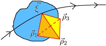
Tetrad variables are a particular way to describe a finite size plasma parcel. The evolution of a parcel’s shape is assigned in the simplest way once it is given the topology of the three-dimensional space within which the continuum moves. In particular, three material points $x_{i=1,2,3}$ are chosen within the parcel, and the displacements

are considered, ${\bf\xi}$ being the centre-of-mass of the parcel (or, in practical applications, e.g. direct numerical simulations or space plasma experiments, any reference material point (Chertkov et al. Reference Chertkov, Pumir and Shraiman1999; Consolini et al. Reference Consolini, Materassi, Marcucci and Pallocchia2015)). The vectors ${\it\rho}_{i=1,2,3}$ form a tetrahedron, referred to as the tetrad, advected by the motion of the plasma. It is worth stressing that the term ‘material’ here, qualifying both ${\bf\xi}$ and the points $x_{i}$ , is particularly relevant, because the dynamics of points following the motion of the fluid within the parcel (and moving together with it) is what we are treating. This allows us to work in Lagrangian variables (Materassi Reference Materassi and Schulz2014, Reference Materassi2015). Figure 2 represents the artist’s vision of the fluid tetrad.

Figure 2.

The fluid tetrad: the curve passing through ${\bf\xi}$ represents the trajectory ‘of the tetrad’, i.e. of the parcel’s centre-of-mass.

The key idea of STD is to consider the velocity of the material point ${\it\rho}_{i}$ as approximated through the (2.1), with the help of tensors in (2.2). If ${\it\delta}\unicode[STIX]{x1D66B}=\unicode[STIX]{x1D66B}(\boldsymbol{x})-\unicode[STIX]{x1D66B}({\bf\xi})$ is correctly interpreted as the Lagrangian derivative with respect to time of the difference between $\boldsymbol{x}$ and ${\bf\xi}$ , this coincides with the Lagrangian time derivative of ${\it\rho}_{i}$ when $\boldsymbol{x}=x_{i}$ is considered; hence

In (2.5) the gradient $\unicode[STIX]{x1D63C}$ is the ‘point-like’ one, $\unicode[STIX]{x1D608}_{{\it\beta}}^{{\it\alpha}}=\partial _{{\it\beta}}\unicode[STIX]{x1D637}^{{\it\alpha}}({\bf\xi})$ , which is calculated for the parcel’s centre-of-mass ${\bf\xi}$ . The tetrad variables are inserted instead to describe the motion of the vertices ${\it\rho}_{i=1,2,3}$ of the tetrad without making any reference to possibly inaccessible point-like measurements. This is done by generalizing (2.5) to any finite scale by considering it as a linear relationship between $\text{d}{\it\rho}_{i}^{{\it\alpha}}/\text{d}t$ and ${\it\rho}_{i}^{{\it\beta}}$ , which is perturbed by a ‘very small’ term $o({\it\rho}_{i})$ . This perturbation tends to be less and less small as larger and larger tetrad sizes are considered. The linear part is represented by a new tetrad variable, namely a $3\times 3$ matrix $\unicode[STIX]{x1D648}$ , so that

What exceeds out of a linear approximation is a ‘small term’ $o({\it\rho})$ in the laminar regime, where fluid quantities can be considered to be space- and time-smooth.

Conversely, in the presence of turbulence, $u_{i}^{{\it\alpha}}$ is not necessarily small, but rather represents an arbitrary fluctuation of the bulk velocity. In this case, the Taylor expansion still holds as the linear approximation of $\text{d}{\it\rho}_{i}^{{\it\alpha}}/\text{d}t$ ,

when the average quantities $\langle \text{d}{\it\rho}_{i}^{{\it\alpha}}/\text{d}t\rangle$ , $\langle {\it\rho}_{i}^{{\it\beta}}\unicode[STIX]{x1D614}_{{\it\beta}}^{{\it\alpha}}\rangle$ and $\langle u_{i}^{{\it\alpha}}\rangle$ are considered, so that

It is convenient to collect the $9$ components of the three vectors ${\it\rho}_{i}$ as $9$ components of a $3\times 3$ matrix ${\bf\varrho}$ , and the noise terms $u_{i}$ in the $3\times 3$ matrix $\unicode[STIX]{x1D650}$ , so that, because

one may collect the three ODEs of (2.7) in matrix form:

Here, the matrix ${\bf\varrho}$ describes the size and shape of the tetrad, i.e. of the parcel. From (2.9) two tensors can be introduced:

which define the anisotropy of the tetrad (were the tetrad formed by usual cartesian axes, as the $\hat{i}$ , ${\hat{j}}$ and $\hat{k}$ are orthonormal directions, this ${\it\bf\Pi}$ would be proportional the $3\times 3$ identity $\mathbf{1}$ , see below).

The tensor $\unicode[STIX]{x1D648}$ in (2.7) and (2.10), namely the coarse-grained version of the velocity gradient $\unicode[STIX]{x1D63C}$ , is a dynamical variable on its own (in the same way as $\unicode[STIX]{x1D63C}$ was in the zero-scale treatment in Viellefosse (Reference Vieillefosse1984)). In the case of MHD, there is also a tensor that is the tetrad version of the magnetic gradient $\unicode[STIX]{x1D655}$ , which is named $\unicode[STIX]{x1D652}$ .

In order to obtain the equations of motion for $\unicode[STIX]{x1D648}$ and $\unicode[STIX]{x1D652}$ , one works on the equations for $\unicode[STIX]{x1D63C}$ and $\unicode[STIX]{x1D655}$ , derived from the visco-resistive MHD equations (Rai Choudhuri Reference Rai Choudhuri1998) with the Lagrangian time-derivatives:

The first step is to derive the effect of applying $\partial _{t}+\unicode[STIX]{x1D66B}\boldsymbol{\cdot }\boldsymbol{\partial }$ to $\unicode[STIX]{x1D63C}$ and $\unicode[STIX]{x1D655}$ , de facto applying a local gradient to both the Lagrangian equations. The incompressibility hypothesis is assumed valid, so that a space-constant mass density may be assumed, and the continuity equation becomes redundant. Moreover, we introduce an auxiliary tensor ${\it\bf\Xi}=\unicode[STIX]{x1D655}-\unicode[STIX]{x1D655}^{\dagger }$ , such that one has the relationship

with electric current density $\boldsymbol{j}$ .

As far as the velocity gradient is concerned, in order for the system to be self-consistent, the constraint $\boldsymbol{\partial }\boldsymbol{\cdot }\unicode[STIX]{x1D66B}=0$ must have null Lagrangian derivative

This implies that the fluid pressure must undergo a certain relationship. In particular one has:

If the above considerations are taken into account, the ODE for $\unicode[STIX]{x1D63C}$ reads:

The tensor $\unicode[STIX]{x1D643}$ in (2.16) contains gradients of gradients which are of the same order of the $o({\it\rho}_{i})$ terms in (2.5). One can neglect these gradient terms if irregular deformations of the tetrad are disregarded. However, in the presence of turbulence, the negligibility of noises can be assumed only on the average. According to the viewpoint of Chertkov et al. (Reference Chertkov, Pumir and Shraiman1999), one may treat $\unicode[STIX]{x1D643}$ as a noise term of assigned statistics, and interpret the ODE in (2.16) as a Langevin equation, in which $\unicode[STIX]{x1D63C}$ and $\unicode[STIX]{x1D655}$ (appearing also through its anti-Hermitian part ${\it\bf\Xi}$ ) couple, and are forced by $\unicode[STIX]{x1D643}$ . The noisy nature of $\unicode[STIX]{x1D643}$ may be justified by considering any derivative operator as ‘undressing the singularities’. Thus, if the medium at hand is turbulent, it is natural to expect that the quantity $({\it\eta}/{\it\rho})\partial ^{2}\unicode[STIX]{x1D608}^{{\it\mu}{\it\nu}}-1/{\it\rho}(\boldsymbol{\partial }\otimes \boldsymbol{\partial }-({\it\delta}^{{\it\mu}{\it\nu}}/3)\partial ^{2})(p+\unicode[STIX]{x1D63D}^{2}/2)+(1/{\it\rho})\unicode[STIX]{x1D609}^{{\it\zeta}}\partial _{{\it\zeta}}\unicode[STIX]{x1D621}^{{\it\mu}{\it\nu}}$ is irregular as a spatio-temporal noise (Frisch Reference Frisch1995).

A very similar reasoning may be adopted for the $\unicode[STIX]{x1D655}$ ODE. Applying the gradient operator to the magnetic equation in (2.12) one may arrive to the matrix form:

Again, the term which renders the ODE ‘inhomogeneous’, may be singled out:

so that the relationships for $\unicode[STIX]{x1D655}$ corresponding to (2.16) can be written:

The two terms in ${\it\Theta}$ represent the resistivity contribution ${\it\zeta}\partial ^{2}\unicode[STIX]{x1D655}$ and the contribution due to inhomogeneous velocity, $\unicode[STIX]{x1D63D}\boldsymbol{\cdot }\boldsymbol{\partial }\unicode[STIX]{x1D63C}$ , respectively. Note that (2.19) precisely states that when ${\it\Theta}=0$ , the magnetic gradient $\unicode[STIX]{x1D655}$ is transported by the operator $[.,\unicode[STIX]{x1D63C}]$ along the motion that $\unicode[STIX]{x1D63C}$ generates à la Lie. The dissipation ${\it\zeta}\partial ^{2}\unicode[STIX]{x1D655}$ and the deformation $\unicode[STIX]{x1D63D}\boldsymbol{\cdot }\boldsymbol{\partial }\unicode[STIX]{x1D63C}$ are the only things which prevent ‘passive transport’ from taking place. These foregoing considerations are consistent with what is well-known of MHD (Rai Choudhuri Reference Rai Choudhuri1998). ${\it\Theta}$ is recognized to be ‘more irregular’ than $[\unicode[STIX]{x1D655},\unicode[STIX]{x1D63C}]$ , hence in (2.19) it can be assimilated to a noise term in the presence of turbulence. Thus, $\unicode[STIX]{x1D655}$ undergoes a proper Langevin equation. Note that, even if we have introduced the possibility of considering turbulence through noise, still no finite size framework has been introduced.

Starting from the zero-size ODEs for $\unicode[STIX]{x1D63C}$ and $\unicode[STIX]{x1D655}$ , one may introduce the equations of motion of tensors that should represent their finite-size versions, namely the variable $\unicode[STIX]{x1D648}$ coarse-graining $\unicode[STIX]{x1D63C}$ and appearing in (2.7), and the magnetic tensor $\unicode[STIX]{x1D652}$ that is the coarse-grained version of $\unicode[STIX]{x1D655}$ . The ODE system for $({\bf\varrho},\unicode[STIX]{x1D648},\unicode[STIX]{x1D652})$ reads:

In (2.20) we use the tensor ${\it\bf\Pi}$ defined in (2.11), this replaces the factor $\mathbf{1}/3$ in the zero-size equations. The tensor quantity ${\it\bf\Pi}$ takes into account of the anisotropy of the tetrad (i.e. of the fluid parcel), while $\mathbf{1}/3$ is obviously isotropic, describing the shape of a point-like entity (the zero-size tetrad).

The noise terms forcing the system are $\unicode[STIX]{x1D650}$ , $\unicode[STIX]{x1D643}$ and ${\it\Theta}$ . These terms can be due both to the fluctuations emerging at scales smaller than the tetrad scale $\ell$ , namely defined as

and to the contact forces exerted by the nearby tetrads.

In order to construct a stochastic theory, the distinction in (2.20) between deterministic terms and noise terms is essential. However in this case, looking at (2.16) and (2.19), it may be fairly obvious. Indeed, as it can be understood from the definitions of $\unicode[STIX]{x1D643}$ and ${\it\Theta}$ , these ‘noises’ are reasonably formed by terms which are not expected to all have the same degree of ‘irregularity’. Here the choice is to adopt a ‘minimal model’ that generalizes the HD assumptions in Chertkov et al. (Reference Chertkov, Pumir and Shraiman1999) to MHD. Thus, the two terms $\unicode[STIX]{x1D643}$ and ${\it\Theta}$ , are subdivided into pure noise terms $h$ and ${\it\theta}$ plus deterministic terms proportional to the deterministic part of the ODE already present. Our assumption is:

Under these hypotheses, the Langevin ODEs describing the STMHD assume the following form:

The system of (2.23) represents the extension of the Lagrangian stochastic tetrad formalism to incompressible MHD. It must be completed with a suitable characterization of the statistics of the noise $\unicode[STIX]{x1D650}$ , $h$ and ${\it\theta}$ , as borrowed from Chertkov et al. (Reference Chertkov, Pumir and Shraiman1999) for neutral fluids. This assumption is crucial, because it enables us to complete the construction of STMHD. Furthermore, choosing the magnetic part to be mathematically ‘isomorphic’ to the velocity components means that the magnetic turbulent fluctuations are assumed to behave like those of velocity, both in terms of energy spectrum and correlations. This choice, defined in (2.29) (please see below), is not the only possible one, but it is the simplest one in order to write a closed form of STMHD.

In the literature there is document much experimental and theoretical evidence that magnetic and velocity fluctuations may follow the same statistical properties (see e.g. Matthaeus & Goldstein Reference Matthaeus and Goldstein1982; Roberts & Goldstein Reference Roberts and Goldstein1991; Verma et al. Reference Verma, Roberts, Goldstein, Ghosh and Stribling1996; Müller & Biskamp Reference Müller and Biskamp2000).

When the Langevin equations (2.23) are re-written in components, they appear as:

Noise $u_{i}^{{\it\alpha}}$ , $h^{{\it\alpha}{\it\beta}}$ and ${\it\theta}^{{\it\alpha}{\it\beta}}$ are assumed to be time- ${\it\delta}$ -correlated and Gaussian. As far as the average values of the noise is concerned, this is assumed to vanish:

(coherently with the assumption that these averages are $o({\it\rho})$ ). In particular, one assumes the correlation functions to be:

all the other possibile combinations (e.g. $\langle u_{i}^{{\it\alpha}}({\it\tau}){\it\theta}^{{\it\gamma}{\it\delta}}({\it\tau}^{\prime })\rangle$ ) being null. The tensors ${\it\Sigma}_{ij}^{(u){\it\alpha}{\it\beta}}({\it\tau})$ , ${\it\Sigma}^{(h){\it\alpha}{\it\beta}{\it\gamma}{\it\delta}}({\it\tau})$ and ${\it\Sigma}^{({\it\theta}){\it\alpha}{\it\beta}{\it\gamma}{\it\delta}}({\it\tau})$ are assumed to be invertible for any ${\it\tau}$ in the non-trivial sense that, for every ${\it\tau}$ , there must exist three tensors ${\it\Sigma}_{{\it\alpha}{\it\beta}}^{(u)-1ij}({\it\tau})$ , ${\it\Sigma}_{{\it\alpha}{\it\beta}{\it\gamma}{\it\delta}}^{(h)-1}({\it\tau})$ and ${\it\Sigma}_{{\it\alpha}{\it\beta}{\it\gamma}{\it\delta}}^{({\it\theta})-1}({\it\tau})$ so that:

Adopting the hypotheses in Chertkov et al. (Reference Chertkov, Pumir and Shraiman1999), one re-writes (2.26) as:

(here $\Vert a\Vert ^{2}\equiv \boldsymbol{a}^{2}=\text{Tr}(a^{\dagger }a)$ is intended for every matrix $\unicode[STIX]{x1D656}$ ).

The form of the correlation matrix ${\it\Sigma}^{({\it\theta}){\it\alpha}{\it\beta}{\it\gamma}{\it\delta}}$ for the magnetic noise ${\it\theta}$ deserves some explanation. In Chertkov et al. (Reference Chertkov, Pumir and Shraiman1999), the hypotheses of (2.28) appears to follow from the assumption that the velocity fluctuations undergo some K41-like cascade theory. This renders stochastic tetrad hydrodynamics (STHD) suitable for describing fluid turbulence within the inertial range of scales (Frisch Reference Frisch1995). Here, we simply assume for $\unicode[STIX]{x1D652}$ that grossly the same rules apply as for $\unicode[STIX]{x1D648}$ , both of these being tensors coarse-grained versions of traceless gradient fields. It appears to be reasonable to suppose:

As anticipated above, this assumption implies that the magnetic fluctuations are statistically equivalent to those of velocity in terms of two time-correlation functions. As in the case of STHD, this limits the validity of our STMHD, under the assumptions of (2.26), (2.28) and (2.29), to the inertial interval of scales, i.e. to a regime of fully developed MHD turbulence. This point is discussed in more detail in §§ 4 and 5.

We now have a system of coupled non-linear Langevin equations, with additive time- ${\it\delta}$ -correlated Gaussian noise terms. In this case, the evolution of ${\bf\varrho}$ , $\unicode[STIX]{x1D648}$ and $\unicode[STIX]{x1D652}$ is probabilistic, and one may wish to calculate the probability to have a given plasma tetrad configuration $({\bf\varrho}(t),\unicode[STIX]{x1D648}(t),\unicode[STIX]{x1D652}(t))$ at a time $t$ conditioned to the knowledge of the tetrad configuration $({\bf\varrho}(t_{0}),\unicode[STIX]{x1D648}(t_{0}),\unicode[STIX]{x1D652}(t_{0}))$ at a certain time $t_{0}<t$ , out of the deterministic and stochastic terms working on the tetrad as in (2.24). The aim of our work is now to introduce a formalism, referred to as functional formalism (FF), rendering this type of calculation possible.

3. The functional formalism of classical statistical dynamics

In 1977, Phythian published the milestone paper (Phythian Reference Phythian1977), in which he constructed a path integral formalism able to produce all the statistical quantities relevant for a classical system undergoing stochastic forces. Such a system, which would undergo a deterministic Cauchy problem in the absence of the random stirring, inherits probabilistic behaviour. The results in Phythian (Reference Phythian1977) are the mathematical tools to obtain the description of the statistical dynamics of a system from that of the stochastic forces.

A classical system, described by dynamical variables ${\it\psi}\in \mathbb{R}^{n}$ and stirred by stochastic noise $f\in \mathbb{R}^{n}$ , is governed by the Langevin equation

In (3.1), ${\it\Lambda}\in C^{\infty }(\mathbb{R}^{n},\mathbb{R}^{n})$ is the deterministic part of the equation. The presence of noise turns the classical dynamics of ${\it\psi}$ into an evolution conditioned time-by-time by the ‘probabilistic choice’ of $f$ . Because of the noise forcing the system, the system dynamics has infinitely many realizations, even for fixed initial conditions. At each of these different evolutions, a statistical weight is attributed, which is determined by the concurrence of the deterministic part and the noise in the Langevin equation (3.1).

In order to evaluate the effect of the stochasticity of $f$ on ${\it\psi}$ , the distribution of this $f$ has to be known. Indeed, if one is interested in properly describing the dynamics of (3.1) between an initial time $t_{0}$ and a later time $t$ , it is necessary to assign the probability distribution functional ${\mathcal{Q}}[f;t_{0},t)$ for each of the infinitely many realizations of $f({\it\tau})$ , where ${\it\tau}\in (t_{0},t]$ . Phythian’s procedure is a way to obtain the correspondent functional ${\mathcal{A}}[{\it\psi};t_{0},t)$ representing the probability that the particular history ${\it\psi}({\it\tau})$ of the dynamical variables takes place in the time interval from $t_{0}$ to  $t$ . The map from ${\mathcal{Q}}[f;t_{0},t)$ to ${\mathcal{A}}[{\it\psi};t_{0},t)$ encodes the fact that ${\it\psi}$ undergoes the full dynamics of (3.1), in which both chance (the noise $f$ ) and necessity (the deterministic part ${\it\Lambda}$ ) are considered (Haken Reference Haken1983): ${\mathcal{Q}}[f;t_{0},t)\stackrel{f,{\it\Lambda}}{\longmapsto }{\mathcal{A}}[{\it\psi};t_{0},t)$ .

In order to construct this map, the distribution ${\mathcal{Q}}[f;t_{0},t)$ is assigned through its characteristic functionals, namely its functional Fourier transform in the space of noise realizations:

Here, $[\text{d}f]$ is the path integral measure in the ambient of noise realizations. From the last equation, the necessity of defining the variables ${\it\chi}\in \mathbb{R}^{n}$ is evident, nominally Fourier-conjugate to the noises $f$ .

The central result in Phythian (Reference Phythian1977) is that, due to the dynamics described in the (3.1), the functional probability distribution that the realizations ${\it\psi}({\it\tau})$ and ${\it\chi}({\it\tau})$ take place in the time interval from $t_{0}$ to $t$ , is given by the expression:

where $N_{0}$ is a normalization constant (see below). Moreover, in (3.3) the symbol $\partial _{{\it\psi}}\cdot {\it\Lambda}$ represents the ‘divergence’ of the field ${\it\Lambda}$ in the phase space of the system described by ${\it\psi}$ , i.e.:

Due to the stochastic ODEs, as in (3.1), Phythian’s formalism deals with the so called Ito–Stratonovich dilemma (Van Kampen Reference Van Kampen1981), which is concerned with the choice made in equation (3) of Phythian (Reference Phythian1977), which refines the Hosokawa and Rosen discrete approximations of path integrals to the second-order instead of the first.

Once the expression of $\unicode[STIX]{x1D63C}[{\it\psi},{\it\chi};t_{0},t)$ has been found, the statistical dynamics of the system described by (3.1) is obtained in a rather simple form. This is also true for the transition probabilities among the different configurations (see, for example, Phythian Reference Phythian1977 or Materassi & Consolini Reference Materassi and Consolini2008). In particular, the probability that the dynamics described in (3.1) gives rise to the transition from an initial configuration ${\it\psi}(t_{0})={\it\psi}_{i}$ to a final one ${\it\psi}(t)={\it\psi}_{f}$ , may be obtained integrating the functional $\unicode[STIX]{x1D63C}[{\it\psi},{\it\chi};t_{0},t)$ over all the realizations ${\it\psi}({\it\tau})$ for ${\it\tau}\in (t_{0},t)$ while keeping ${\it\psi}(t_{0})$ fixed as ${\it\psi}_{i}$ , and ${\it\psi}(t)$ fixed as ${\it\psi}_{f}$ , and ${\it\chi}({\it\tau})$ for ${\it\tau}\in [t_{0},t]$ :

In a more compact way, the foregoing expression can be written as

where the symbol $\langle F\rangle$ indicates the average value of $F$ over the histories, i.e. $\langle F\rangle =\int [\text{d}{\it\chi}]\int [\text{d}{\it\psi}]\unicode[STIX]{x1D63C}F$ , and $F=1$ in (3.6).

The explicit calculation of $\unicode[STIX]{x1D63C}[{\it\psi},{\it\chi};t_{0},t)$ needs an expression for $C[{\it\chi};t_{0},t)$ , which is easy to obtain in the particular case when the noise components $f^{{\it\alpha}}$ have a Gaussian distribution $q$ with an assigned correlation function given by:

The matrix ${\it\bf\Sigma}\in \mathbb{R}^{n,n}$ in (3.7) is assumed to be invertible, and only its symmetric part play any role because it will be saturated with a symmetric tensor. Thus the distribution of the noise vector at a fixed time $f({\it\tau})$ reads:

In all of these distributions, the functions $f_{0}^{{\it\gamma}}({\it\tau})$ represent the expected value of the noise $f^{{\it\gamma}}({\it\tau})$ . The distribution (3.8) is correctly normalized, i.e.

Moreover, the pre-factor $C[{\it\chi};t_{0},t)$ can be written as

This expression enables us to calculate explicitly the kernel as a functional of ${\it\psi}$ and ${\it\chi}$ , by placing (3.10) into (3.3), as done in appendix B. The kernel, expressed as a functional of dynamical variables and stochastic momenta, is given by:

The expression of (3.11) is, to some extent, not physical, because, while the ${\it\psi}$ variables mean ‘something physical’ for the system, the ${\it\chi}$ variables are just what remains of the noise. If one integrates out the stochastic momenta in $\unicode[STIX]{x1D63C}[{\it\psi},{\it\chi};t_{0},t)$ , then a more intuitive form of the kernel is obtained,

In the case of Gaussian time- ${\it\delta}$ -correlated noises, ${\mathcal{A}}$ can be expressed (see appendix C for computational details):

The kernel ${\mathcal{A}}$ may be expressed in terms of a functional depending on the evolution of ${\it\psi}({\it\tau})$ , namely the stochastic action $S[{\it\psi}]$ , so that the kernel acquires the form:

where the stochastic action $S[{\it\psi};t_{0},t)$ is given by the following expression:

If the Gaussian noise has zero mean, i.e. if

then the stochastic action reduces to the expression:

The expressions (3.14) and (3.15), or (3.17) with null average noise, are the crucial ones through which one classical system, with dynamics forced by Gaussian time- ${\it\delta}$ -correlated noise, is turned into a stochastic system treated via a functional formalism.

4. The stochastic action for tetrad MHD

Now we are in a position to put together the STMHD findings presented in § 2 with Phythian’s functional formalism discussed in § 3. To this end, we need to express the action of (3.17) with the assumptions made on the noise statistics by means of (2.26), (2.28) and (2.29). However, it is important to remark that the STMHD presented here is suitable for describing the finite scale statistical dynamics of incompressible MHD turbulence only when the aforementioned assumptions hold for the velocity and magnetic fluctuations. In particular, this is the case of velocity fluctuations that satisfy the K41 results in the inertial range (and the same is expected for magnetic field fluctuations $\unicode[STIX]{x1D63D}$ occurring in turbulent MHD systems) so that a condition on the interval range of scales where the previous framework can be simply set. The other hypotheses on $\langle h^{{\it\alpha}{\it\beta}}({\it\tau})h^{{\it\gamma}{\it\delta}}({\it\tau}^{\prime })\rangle$ and $\langle {\it\theta}^{{\it\alpha}{\it\beta}}({\it\tau}){\it\theta}^{{\it\gamma}{\it\delta}}({\it\tau}^{\prime })\rangle$ could be suitable to describe other regimes. This is a point that will be investigated in future work.

The inverse tensors of cross correlation matrices in (2.28) and (2.29) are calculated in appendix D. However, the inverse matrix of the first cross-correlation tensor can be written as follows:

while, as far as the cross-correlation tensor in (2.28) is concerned, the arguments in appendix D imply that, de facto, we are speaking about inverting the identical application of $\mathbb{R}^{3,3}$ onto $\mathbb{R}^{3,3}$ . Thus, one may write:

Moreover, the inversion of the cross correlation tensor for the noise ${\it\theta}$ leads to the expression:

The two conditions in the (2.26) and (2.25) allow to use the relationship in (3.17) to calculate the stochastic action of the Tetrad MHD.

The vector of dynamical variables ${\it\psi}$ is:

where one has to remember that $\unicode[STIX]{x1D648}$ and $\unicode[STIX]{x1D652}$ are tensors of components $\unicode[STIX]{x1D614}^{{\it\alpha}{\it\beta}}$ and $\unicode[STIX]{x1D61E}^{{\it\alpha}{\it\beta}}$ . Moreover, the deterministic parts of the Langevin equations can be written as:

We then start by calculating the ‘divergence’ $\partial _{{\it\psi}}\cdot {\it\Lambda}$ of ${\it\Lambda}$ in the phase space of ${\it\psi}$ , obtaining:

Detailed calculations can be found in appendix C. Thus, this ‘divergence’ can be written in the form:

In order to complete the calculation of the stochastic functional ${\mathcal{A}}[{\it\psi};t_{0},t)$ one has to calculate the expression $(\dot{{\it\psi}}-{\it\Lambda})^{\dagger }\cdot {\it\Sigma}^{-1}\cdot (\dot{{\it\psi}}-{\it\Lambda})$ . This is done, in detail, in the appendix D. The obtained result is:

after placing the terms (D 13) in (D 15).

The stochastic action for the tetrad MHD may be calculated considering the relationships of (4.7) and (4.8) in (3.17):

With the aforementioned stochastic action, the transition kernel of the tetrad MHD results in the form:

The kernel ${\mathcal{A}}[{\bf\varrho},\unicode[STIX]{x1D648},\unicode[STIX]{x1D652};t_{0},t)$ has a paramount role in the construction of any quantity relevant for the statistical dynamics of the STMHD. In § 3 we have already seen how to calculate the transition probability between an initial configuration of the system ${\it\psi}(t_{0})={\it\psi}_{i}$ and a final one ${\it\psi}(t)={\it\psi}_{f}$ . In this case, the transition would be

and the probability for it to take place is:

where the kernel of (4.10) and the stochastic action of (4.9) have been used.

If the initial, or final, configuration is not fully observed, e.g. if we want to calculate the transition ${\bf\varrho}_{i}\mapsto {\bf\varrho}_{f}$ regardless of the configuration of the magnetic and kinetic gradient, one simply avoids fixing $\unicode[STIX]{x1D648}_{f}$ , $\unicode[STIX]{x1D652}_{f}$ , $\unicode[STIX]{x1D648}_{i}$ and $\unicode[STIX]{x1D652}_{i}$ in (4.12). For instance, one has

As explained in Phythian (Reference Phythian1977), the functional formalism allows us to calculate the $N$ times correlation functions. In particular, the formula of the $N$ -fold correlation function ${\mathcal{G}}({\it\psi}^{{\it\alpha}_{1}}(t_{1}),\ldots ,{\it\psi}^{{\it\alpha}_{N}}(t_{N}))$ , among $N$ components of ${\it\psi}$ taken at $N$ different times, is defined as:

In the STMHD case, the calculation of the correlation between two components of $\unicode[STIX]{x1D648}$ at two different times, e.g. $t_{1}$ and $t_{2}$ , both within $(t_{0},t)$ , consists in the computation of:

Again, this may be used to calculate any correlation function between any components of the STMHD configuration. Furthermore, its analytical form, as derived from (4.10) when it is possible to perform this calculation, would allow us to predict theoretically the time resolved self- or mutual-correlation measurements.

In forthcoming studies, use of the closed form of (4.10) will be made to reproduce what is already known in STHD and to extend the turbulence theory results to STMHD, following the path explained in § 5. The formalism just developed in this paper is represented here in an initial stage, which will be the core of a systematic application wherever incompressible MHD applies. Of course, turbulent solar wind, magnetospheric and boundary layer plasmas are important candidates that will be considered. In particular, in the case of incompressible MHD turbulence, Elsässer variables could be more appropriate than $\unicode[STIX]{x1D66B}$ and $\unicode[STIX]{x1D63D}$ when application to a solar wind context is considered. The description of the above path integral approach in terms of Elsässer variable will be formalized in a successive study. The mathematical core of the present paper is simply aimed at being broader than any specific set of variables.

5. Summary and conclusions

The present paper has focussed on the introduction of the stochastic tetrad in MHD turbulence theory. The main advantages of this approach are:

1. (1) keeping the method as close as possible to material particle dynamics;

2. (2) promoting the plasma parcel’s size to the role of a dynamical variable;

3. (3) accepting the stochastic nature of turbulence at the macroscopic level as a result of smaller scale fluctuations and forces exerted by the nearby plasma.

The approach chosen here to meet those requirements is to consider the Lagrangian dynamics of tetrads in fluids, as described in Chertkov et al. (Reference Chertkov, Pumir and Shraiman1999), and to generalize it to plasmas. This extension includes a new coarse-grained gradient tensor $\unicode[STIX]{x1D652}$ representing the tetrad version of $\boldsymbol{\partial }\otimes \unicode[STIX]{x1D63D}$ and the noises forcing the new magnetic variable. As in Chertkov’s theory (Chertkov et al. Reference Chertkov, Pumir and Shraiman1999), here, all the noises are considered time- ${\it\delta}$ -correlated and Gaussian. This means that the fluctuations pertain to the inertial scale range of the fully developed isotropic turbulence, both for $\unicode[STIX]{x1D66B}$ - and $\unicode[STIX]{x1D63D}$ -turbulence.

The Langevin equations (2.23) for the tetrad variables $({\bf\varrho},\unicode[STIX]{x1D648},\unicode[STIX]{x1D652})$ show clearly how the kinetic and magnetic tensors interact. The $\unicode[STIX]{x1D648}$ tensor dynamics is fully determined by both fluid and Lorentz forces, through terms involving the anti-Hermitian part ${\it\bf\Xi}=\unicode[STIX]{x1D652}-\unicode[STIX]{x1D652}^{\dagger }$ , which is namely the dual of the electric density currents. However, $\unicode[STIX]{x1D652}$ would be purely dragged by $\unicode[STIX]{x1D648}$ , i.e. by the matter motion, unless of the higher-order derivatives of $\unicode[STIX]{x1D66B}$ and the dissipative effects unfreezing the $\unicode[STIX]{x1D63D}$ -flux through the plasma.

The minimal model hypothesis is done in (2.22), which is essentially the same result as in Chertkov et al. (Reference Chertkov, Pumir and Shraiman1999). Here, the forcing terms are considered to be the sum of the pure noise terms ( $\unicode[STIX]{x1D650}$ , $h$ and ${\it\theta}$ ) and the deterministic corrections proportional to the deterministic free parts.

The statistical properties of the tetrad system $({\bf\varrho},\unicode[STIX]{x1D648},\unicode[STIX]{x1D652})$ may be deduced either through a Fokker–Planck equation, as Chertkov et al. did for the HD turbulence, or via a Martin–Siggia–Rose-like mechanism (Martin, Siggia & Rose Reference Martin, Siggia and Rose1973), namely via a functional formalism inspired by what is presented in Phythian (Reference Phythian1977). This is the approach we have chosen here. As it is usually done in quantum mechanics (Feynman & Hibbs Reference Feynman and Hibbs1965), an action functional $S[{\bf\varrho},\unicode[STIX]{x1D648},\unicode[STIX]{x1D652};t_{0},t)$ is introduced, whose exponentiation gives the probability for the particular evolution $({\bf\varrho}({\it\tau}),\unicode[STIX]{x1D648}({\it\tau}),\unicode[STIX]{x1D652}({\it\tau}))$ to occur between $t_{0}$ and $t$ . This stochastic action is calculated for full incompressible MHD, and reported in (4.9).

Once the probabilistic weight ${\mathcal{A}}[{\bf\varrho},\unicode[STIX]{x1D648},\unicode[STIX]{x1D652};t_{0},t)=N_{0}\exp (-S[{\bf\varrho},\unicode[STIX]{x1D648},\unicode[STIX]{x1D652};t_{0},t))$ is calculated, it becomes possible to evaluate any statistically relevant quantity for the stochastic system. For instance, the kernel ${\mathcal{A}}[{\bf\varrho},\unicode[STIX]{x1D648},\unicode[STIX]{x1D652};t_{0},t)$ in (4.12) is used to find the transition probability between a given initial and a given final STMHD configuration, while in (4.15) the use of it is suggested to calculate the mutual correlation between the values of two components of the tensor $\unicode[STIX]{x1D648}$ at two different times.

The stochastic action $S$ in (4.9) contains three quadratic terms, which are coupled via the inverse cross-correlations of noise ${\it\Sigma}^{-1}$ , and one term $(1-{\it\alpha}_{v})\text{Tr}({\it\bf\Pi}({\bf\varrho})\boldsymbol{\cdot }\unicode[STIX]{x1D648})$ which represents the coupling between the anisotropy of the tetrad and the velocity gradient. We remark that there is a convergence between the STMHD action determined via Phythian’s functional formalism and the Green function found in Chertkov et al. (Reference Chertkov, Pumir and Shraiman1999) from the Fokker–Planck equation, derived using the system (2.23).

The introduction of the kernel ${\mathcal{A}}[{\bf\varrho},\unicode[STIX]{x1D648},\unicode[STIX]{x1D652};t_{0},t)$ is just the starting point of our program of stochastic tetrad MHD, which is intended to cast new light on plasma turbulence. In particular, we believe that this is the right approach to characterise the inherent inhomogeneity, stochasticity and intermittent nature of turbulent plasmas. Indeed, moving from the closed expressions for the statistical weight of histories, we can use the FF for STMHD to make practical predictions of physical quantities, as, for instance, those illustrated in § 4 and many others. The closed forms for quantities of interest can be then compared with the results of direct numerical simulations of how the local topology of a turbulent MHD plasma evolves. An extension to plasmas of the results in Dallas & Alexakis (Reference Dallas and Alexakis2013) will be attempted in future work, so that that it will be possible to re-interpret the results via this FF.

Experimental data from space plasmas can be used also in order to validate, criticize and improve the STMHD results, as, for instance, those presented in Volwerk et al. (Reference Volwerk, Vörös, Baumjohann, Nakamura, Runov, Zhang, Glassmeier, Treumann, Klecker and Balogh2004) and in Vörös et al. (Reference Vörös, Baumjohann, Nakamura, Volwerk, Runov, Zhang, Eichelberger, Treumann, Georgescu and Balogh2004). The study of what our multi-scale formalism may teach about space plasma dynamics and topology can finally be of importance to forthcoming and/or future space missions aimed at documenting the role that the inter-scale dynamics takes in turbulent plasmas.

We would like comment with a comparison between the present tetrad dynamics and the use of quaternionic quantities to describe the evolution of a fluid Lagrangian parcel (Gibbon & Holm Reference Gibbon and Holm2007). A tetrad is a ‘more flexible’ description than a quaternion because the tetrahedron shape may be whichever, and is not purely related to the orthonormality conditions. This aspect of the tetrad approach is crucial to compare theoretical results with multi-probe measurements (e.g. the ESA-CLUSTER mission and the NASA-Magnetospheric Multiscale (MMS) mission in the space plasma context).