2 Model

Consider a legislature of $K$ legislators voting on $N$ bills. Assume legislators have unidimensional spatial preferences and vote sincerely according to the stochastic utility function given by

(1) $$\begin{eqnarray}\displaystyle u_{i}\left(v_{ij}=1\right) & = & \displaystyle f\left(x_{i}-y_{j1}\right)+\unicode[STIX]{x1D701}_{ij1}\end{eqnarray}$$

(2) $$\begin{eqnarray}\displaystyle u_{i}\left(v_{ij}=0\right) & = & \displaystyle -f\left(x_{i}-y_{j0}\right)+\unicode[STIX]{x1D701}_{ij0}\end{eqnarray}$$

(3) $$\begin{eqnarray}\displaystyle \unicode[STIX]{x1D701}_{ij1},\unicode[STIX]{x1D701}_{ij0} & \stackrel{iid}{{\sim}} & \displaystyle G_{j}\end{eqnarray}$$

where $v_{ij}$ is the vote of legislator $i$ on bill $j$ , $v_{ij}=1$ indicates a vote of “yea,” $v_{ij}=0$ indicates a vote of “nay,” $y_{j1}$ is the policy outcome of the bill, $y_{j0}$ is the status quo, $x_{i}$ is the ideal point of legislator, $\unicode[STIX]{x1D701}_{ij1}$ and $\unicode[STIX]{x1D701}_{ij0}$ are stochastic errors, and $G_{j}$ is the joint distribution of $\unicode[STIX]{x1D701}_{ij1}$ and $\unicode[STIX]{x1D701}_{ij0}$ for bill $j$ . Assume that $f$ is a strictly concave function with a maximum at zero.Footnote ⁶ Further, assume that the errors, $\unicode[STIX]{x1D701}_{ij1}$ and $\unicode[STIX]{x1D701}_{ij0}$ , are independent across bills and legislators and identically distributed for each bill. Finally, assume legislators vote “yea” when indifferent.Footnote ⁷ Note that they only differ in their ideal points, $x_{i}$ , and not in $f$ , which is assumed to be the same for all legislators. Note also that the distribution $G_{j}$ of the stochastic utility components, $\unicode[STIX]{x1D701}_{ij1}$ and $\unicode[STIX]{x1D701}_{ij0}$ , is assumed to be the same for all legislators for any given bill but can vary across bills.

The probability of legislator $i$ voting “yea” on bill $j$ is given by

(4) $$\begin{eqnarray}\displaystyle \text{Pr}\left(v_{ij}=1\right) & = & \displaystyle \text{Pr}\left(u_{i}\left(v_{ij}=1\right)\geqslant u_{i}\left(v_{ij}=0\right)\right)\nonumber\\ \displaystyle & = & \displaystyle \text{Pr}\left(f\left(x_{i}-y_{j1}\right)-f\left(x_{i}-y_{j0}\right)\geqslant \unicode[STIX]{x1D701}_{ij0}-\unicode[STIX]{x1D701}_{ij1}\right).\end{eqnarray}$$

Let $H_{j}$ be the cumulative distribution function of $\unicode[STIX]{x1D701}_{ij0}-\unicode[STIX]{x1D701}_{ij1}~\left(H_{j}\left(z\right)=\text{Pr}\left(\unicode[STIX]{x1D701}_{ij0}-\unicode[STIX]{x1D701}_{ij1}\leqslant z\right)\right)$ . Thus,

(5) $$\begin{eqnarray}\text{Pr}\left(v_{ij}=1\right)=H_{j}\left(f\left(x_{i}-y_{j1}\right)-f\left(x_{i}-y_{j0}\right)\right).\end{eqnarray}$$

The results in this paper rest on the implication of this model that $\text{Pr}\left(v_{ij}=1\right)$ is monotonic in $x_{i}$ . It is also worth noting that, if $y_{j0}\neq y_{j1}$ and $H$ is strictly increasing, then $\text{Pr}\left(v_{ij}=1\right)$ is strictly monotonic in $x_{i}$ . These two conditions require only that the policy outcome of the bill differs from the status quo and that the error distribution has support over the entire real line.

The following theorem establishes these results:

This model bares some similarity to a nonparametric item-response theory model developed by Mokken (Reference Mokken1971): the monotone homogeneity model. The crucial difference is that the above model assumes that the probability of a certain vote choice is merely a monotonic function of a legislator’s ideal point and can, thus, be either nondecreasing or nonincreasing. In contrast, the monotone homogeneity model assumes a priori knowledge of which answer is correct and, therefore, nondecreasing in a student’s ability. Unfortunately, such a simple approach is not applicable to the more general problem of nonparametric ideal-point estimation, where researchers cannot be presumed to know whether a “yea” vote is the more “conservative” or “liberal” vote choice.Footnote ⁸ Mokken’s (Reference Mokken1971) approach also requires an absence of missing values, further limiting its relevance to analyzing roll-call data.

3 Estimation

Under the model described in the previous section, knowing which of two legislators is to the right of the other does not tell us which is more likely to vote “yea” on a given bill. This is in sharp contrast to the monotone heterogeneity model, where knowing which student has higher ability directly implies which is more likely to answer a question correctly.

Most approaches to ideal-point estimation have addressed the need to know the polarity of each bill and other bill-specific parameters by simultaneously estimating these parameters.Footnote ⁹ Introducing these parameters can complicate both estimation and inference. For example, maximum likelihood estimators may be inconsistent when such parameters are included (Neyman and Scott Reference Neyman and Scott1948). Further, even aside from these complications, estimating the relationship between ideal points and vote probabilities is impractical here because the parameter space is infinite.

In this paper, I adopt a different approach that avoids estimating bill-specific parameters. The key insight for both estimation and inference is that, while we cannot learn much from the votes of a pair of legislators alone, the votes of two pairs can be informative. For any two pairs of legislators, if we condition on each pair containing one “yea” vote and one “nay” vote, then the conditional probability that the more conservative of the legislators in each pair voted together and the more liberal legislators in each pair voted together is greater than the probability that the more liberal of the legislators of each pair voted with the more conservative of the other.

More formally, if $x_{i}<x_{k}$ and $x_{\ell }<x_{m}$ , then either  $\text{Pr}\left(v_{kj}=1\right)\,-\,\text{Pr}\left(v_{ij}=1\right)\geqslant 0$ and $\text{Pr}\left(v_{mj}=1\right)-\text{Pr}\left(v_{\ell j}=1\right)\geqslant 0$ or $\text{Pr}\left(v_{kj}=1\right)-\text{Pr}\left(v_{ij}=1\right)\leqslant 0$ and $\text{Pr}\left(v_{mj}=1\right)-\text{Pr}\left(v_{\ell j}=1\right)\leqslant 0$ . For notational convenience, let $p_{i}=\text{Pr}\left(v_{ij}=1\right)$ and $q_{i}=\text{Pr}\left(v_{ij}=0\right)=1-\text{Pr}\left(v_{ij}=1\right)$ . In either case,

(14) $$\begin{eqnarray}\displaystyle 0 & {\leqslant} & \displaystyle \left(p_{k}-p_{i}\right)\left(p_{m}-p_{\ell }\right)\end{eqnarray}$$

(15) $$\begin{eqnarray}\displaystyle 0 & {\leqslant} & \displaystyle \left(p_{k}-p_{i}p_{k}-p_{i}+p_{i}p_{k}\right)\left(p_{m}-p_{\ell }p_{m}-p_{\ell }+p_{\ell }p_{m}\right)\end{eqnarray}$$

(16) $$\begin{eqnarray}\displaystyle 0 & {\leqslant} & \displaystyle \left(\left(1-p_{i}\right)p_{k}-p_{i}\left(1-p_{k}\right)\right)\left(\left(1-p_{\ell }\right)p_{m}-p_{\ell }\left(1-p_{m}\right)\right)\end{eqnarray}$$

(17) $$\begin{eqnarray}\displaystyle 0 & {\leqslant} & \displaystyle \left(1-p_{i}\right)p_{k}\left(\left(1-p_{\ell }\right)p_{m}-p_{\ell }\left(1-p_{m}\right)\right)-p_{i}\left(1-p_{k}\right)\left(\left(1-p_{\ell }\right)p_{m}-p_{\ell }\left(1-p_{m}\right)\right)\end{eqnarray}$$

(18) $$\begin{eqnarray}\displaystyle 0 & {\leqslant} & \displaystyle q_{i}p_{k}\left(q_{\ell }p_{m}-p_{\ell }q_{m}\right)-p_{i}q_{k}\left(q_{\ell }p_{m}-p_{\ell }q_{m}\right).\end{eqnarray}$$

So,

(19) $$\begin{eqnarray}\displaystyle p_{i}q_{k}\left(q_{\ell }p_{m}-p_{\ell }q_{m}\right) & {\leqslant} & \displaystyle q_{i}p_{k}\left(q_{\ell }p_{m}-p_{\ell }q_{m}\right)\end{eqnarray}$$

(20) $$\begin{eqnarray}\displaystyle p_{i}q_{k}q_{\ell }p_{m}-p_{i}q_{k}p_{\ell }q_{m} & {\leqslant} & \displaystyle q_{i}p_{k}q_{\ell }p_{m}-q_{i}p_{k}p_{\ell }q_{m}\end{eqnarray}$$

(21) $$\begin{eqnarray}\displaystyle p_{i}q_{k}q_{\ell }p_{m}+q_{i}p_{k}p_{\ell }q_{m} & {\leqslant} & \displaystyle p_{i}q_{k}p_{\ell }q_{\ell }+q_{i}p_{k}q_{\ell }p_{m}.\end{eqnarray}$$

By independence of $v_{ij}$ , $v_{kj}$ , $v_{\ell j}$ , and $v_{mj}$ , this implies

(22) $$\begin{eqnarray}\displaystyle \text{Pr}\left(v_{ij}=v_{mj}\wedge v_{ij}\neq v_{kj}\wedge v_{\ell j}\neq v_{mj}\right) & {\leqslant} & \displaystyle \text{Pr}\left(v_{kj}=v_{mj}\wedge v_{ij}\neq v_{kj}\wedge v_{\ell j}\neq v_{mj}\right)\end{eqnarray}$$

(23) $$\begin{eqnarray}\displaystyle \frac{\text{Pr}\left(v_{ij}=v_{mj}\wedge v_{ij}\neq v_{kj}\wedge v_{\ell j}\neq v_{mj}\right)}{\text{Pr}\left(v_{ij}\neq v_{kj}\wedge v_{\ell j}\neq v_{mj}\right)} & {\leqslant} & \displaystyle \frac{\text{Pr}\left(v_{kj}=v_{mj}\wedge v_{ij}\neq v_{kj}\wedge v_{\ell j}\neq v_{mj}\right)}{\text{Pr}\left(v_{ij}\neq v_{kj}\wedge v_{\ell j}\neq v_{mj}\right)}\end{eqnarray}$$

(24) $$\begin{eqnarray}\displaystyle \text{Pr}\left(v_{ij}=v_{mj}\mid v_{ij}\neq v_{kj}\wedge v_{\ell j}\neq v_{mj}\right) & {\leqslant} & \displaystyle \text{Pr}\left(v_{kj}=v_{mj}\mid v_{ij}\neq v_{kj}\wedge v_{\ell j}\neq v_{mj}\right).\end{eqnarray}$$

Thus, if we consider only the votes where $v_{ij}\neq v_{kj}$ and $v_{\ell j}\neq v_{mj}$ , the expected count of votes on which $v_{kj}=v_{mj}$ is greater than or equal to the expected count of votes on which $v_{kj}=v_{mj}$ . Let

(25) $$\begin{eqnarray}v_{im\mid k\ell }^{j}=\left\{\begin{array}{@{}ll@{}}1\quad & \text{if }v_{kj}=v_{mj}\wedge v_{ij}\neq v_{kj}\wedge v_{\ell j}\neq v_{mj}\\ 0\quad & \text{otherwise}\end{array}\right.\end{eqnarray}$$

so that $v_{im\mid k\ell }^{j}$ indicates that legislators $i$ and $m$ voted together and legislators $k$ and $\ell$ voted together but each pair voted differently from the other on bill $j$ . Under weak regularity conditions,Footnote ¹⁰ the law of large numbers implies that

(26) $$\begin{eqnarray}\lim _{N\rightarrow \infty }\text{Pr}\left(\mathop{\sum }_{j=1}^{N}v_{km\mid i\ell }^{j}>\mathop{\sum }_{j=1}^{N}v_{im\mid k\ell }^{j}\right)=1.\end{eqnarray}$$

Thus, if we consider only bills for which legislators $i$ and $k$ voted differently and legislators $\ell$ and $m$ voted differently, the fraction of these in which legislators $k$ and $m$ voted together should be greater than $\frac{1}{2}$ .

Let $\prec$ be the binary relation giving the true ordering of the ideal points where $i\prec k$ indicates that legislator $i$ is to the left of legislator $k$ (i.e., $x_{i}<x_{k}$ ). Let $\hat{\prec }$ be the binary relation giving the estimated ordering relation where $i\,\hat{\prec }\,k$ indicates that legislator $i$ is estimated to be to the left of legislator $k$ . If $\hat{\prec }$ is a consistent estimator of $\prec$ , then

(27) $$\begin{eqnarray}\mathop{\sum }_{j=1}^{N}v_{km\mid i\ell }^{j}>\mathop{\sum }_{j=1}^{N}v_{im\mid k\ell }^{j}\end{eqnarray}$$

must imply $i\hat{\prec }k\Leftrightarrow \ell \hat{\prec }m$ for sufficiently large $N$ and all $i\neq k\neq \ell \neq m$ . Thus, a consistent estimator will minimize $\sum _{j=1}^{N}v_{km\mid i\ell }^{j}-v_{im\mid k\ell }^{j}$ for sufficiently large $N$ and all $i\neq k\neq \ell \neq m$ such that $i\hat{\prec }k\wedge \ell \hat{\prec }m$ . Therefore, it also minimizes the sum of this quantity over all possible groups of legislators satisfying $i\hat{\prec }k\wedge \ell \hat{\prec }m$ ,

(28) $$\begin{eqnarray}\mathop{\sum }_{i\neq k\neq \ell \neq m}\mathop{\sum }_{j=1}^{N}\left(v_{km\mid i\ell }^{j}-v_{im\mid k\ell }^{j}\right)\mathbb{1}\left(i\hat{\prec }k\wedge \ell \hat{\prec }m\right)\end{eqnarray}$$

where $\mathbb{1}\left(x\right)$ is the indicator function ( $\mathbb{1}\left(x\right)=1$ if $x$ is true and $0$ otherwise) for sufficiently large $N$ .

This suggests choosing as an estimator the relation $\hat{\prec }$ that minimizes Formula (28). Identifiability also requires constraining the order of two legislators. Given this constraint and the necessary regularity condition (see footnote 25), this estimator is unique, at least for sufficiently large $N$ , and therefore consistent.

Computing this estimator is difficult. There is no apparent alternative to an exhaustive search, but this requires considering $\frac{1}{2}K!$ possible orderings for $K$ legislators and summing over $2\binom{K}{4}$ choices of legislators satisfying $i\hat{\prec }k\wedge \ell \hat{\prec }m$ . Thus, computing Formula (28) for $\frac{1}{2}K!$ possible orderings requires computing the inner sum of Formula (28) $K!\binom{K}{4}$ times.Footnote ¹¹ This is feasible for a sufficiently small number of legislators, but cases where $n>10$ seem impractical.Footnote ¹²

Thus, for larger numbers of legislators, a different approach is necessary. However, if we choose two legislators, $\ell$ and $m$ , and consider only the votes in which they disagree, then the remaining $K-2$ can be ordered based on the fraction of the votes in which each voted with $m$ instead of $\ell$ . As was the case when we considered two pairs of legislators, the expectation of the fraction of the votes in which each voted with $m$ is increasing in their ideal points if $\ell \prec m$ and decreasing if $m\prec \ell$ .

If we repeat this process for each possible pair of legislators, we then only need to combine these orderings of each of the $\binom{K}{2}$ sets of legislators into a single ordering for all legislators. Doing so can be done by creating a $\binom{K}{2}\times K$ matrix with each row giving a numeric ranking of a different set of $K-2$ with the two held-out legislators given the mean rank, then mean-centering each row, and finally performing a singular value decomposition (SVD). If all rankings on each subset of $\binom{K}{2}$ legislators are correct, as will be true asymptotically, the order of the values in the first right-singular vector (i.e., the one corresponding to the largest singular value) should agree with the true ordering of the ideal points up to a reversal. Further, if it is too burdensome to compute rankings for all $\binom{K}{2}$ groups of legislators, this can be replaced by a smaller number of groups of $K-2$ chosen at random.

Although this estimator is also consistent under the same regularity conditions, it can only be based on roll-call items with no missing votes. In contrast, the alignment of two pairs of legislators can be computed using only the votes of those four legislators. Thus, the original estimator proposed in this paper is able to use any roll-call items in which at least four legislators voted. Since roll-call data often contain few or no items without any missing votes, the SVD-based approach as outlined above is not feasible but can be modified by computing the fraction of times one legislator agrees with another with missing values imputed by the mean agreement on nonmissing votes. This estimator need not be consistent but is likely to return similar results to the other, consistent estimators provided the fraction of missing votes is not too large.

4 Inference

Suppose we have two groups of roll-call items and wish to test whether a single ideological dimension could explain voting on both groups—or, equivalently, we wish to test whether the legislators’ ideal points maintained the same ordering on both items. The same approach used for estimation of choosing two pairs of legislators and focusing on those votes where each pair disagrees also provides a natural approach for performing inference. Indeed, the pairs-of-pairs approach is, in some ways, a more natural fit to inference than estimation and will provide a means to test the equal-ordering hypothesis without needing to estimate an ordering or to impose identifiability constraints.

Consider a two-sample extension of the model in Section 2 in which $K$ legislators vote on two separate groups of bills, the first consisting of $N_{A}$ items and the second of $N_{B}$ . Let $A$ be the set of indices of the first group, such that bill $j$ is in group A if and only if $j\in A$ and let $B$ be the set of indices for group B, where $A$ and $B$ are disjoint. Assume the order of the legislators’ ideal points is given by the binary relation $\prec _{A}$ for the first group of $N_{A}$ bills and $\prec _{B}$ for the second.Footnote ¹³

Finally, although most of the results in this section can be derived without this assumption, it will simplify matters to assume that the bill-specific parameters ( $y_{j1}$ , $y_{j0}$ , and $G_{j}$ ) are jointly independently and identically distributed within each group, with distinct distributions for the bill parameters for each group and with no restrictions placed on the forms of these distributions. Thus, the bill parameters for one group may be drawn from a quite different distribution than the bill parameters in the other.

I aim to construct a test of the null hypothesis that the legislators have the same ordering on both groups—that is, that $i\prec _{A}k\Leftrightarrow i\prec _{B}k$ for all $i$ and $k$ .

Let

(29) $$\begin{eqnarray}\unicode[STIX]{x1D70B}_{km\mid i\ell }^{\left(A\right)}=E_{A}\left[\text{Pr}\left(v_{ij}=v_{mj}\mid v_{ij}\neq v_{kj}\wedge v_{\ell j}\neq v_{mj}\right)\right]\end{eqnarray}$$

indicate the marginal probability that $\text{Pr}\left(v_{kj}=v_{mj}\mid v_{ij}\neq v_{kj}\wedge v_{\ell j}\neq v_{mj}\right)$ marginalized over the distribution of the bill parameters for group A, with $\unicode[STIX]{x1D70B}_{km\mid i\ell }^{\left(B\right)}$ defined analogously for group B. Thus, given the number of votes in which $v_{ij}\neq v_{kj}\wedge v_{\ell j}\neq v_{mj}$ , the conditional distribution for the number of votes in which $v_{kj}$ also equals $v_{mj}$ (i.e., the sum of $v_{km\mid i\ell }^{j}$ over $A$ ) is the sum of $\sum _{j\in A}v_{km\mid i\ell }^{j}+v_{im\mid k\ell }^{j}$ trials each with success probability $\unicode[STIX]{x1D70B}_{km\mid i\ell }^{\left(A\right)}$ , where, as in the previous section, $v_{km\mid i\ell }^{j}=\mathbb{1}\left(v_{kj}=v_{mj}\wedge v_{ij}\neq v_{kj}\wedge v_{\ell j}\neq v_{mj}\right)$ . Thus, the distribution is given by

(30) $$\begin{eqnarray}\mathop{\sum }_{j\in A}v_{km\mid i\ell }^{j}\sim \text{Binomial}\left(\mathop{\sum }_{j\in A}v_{km\mid i\ell }^{j}+v_{im\mid k\ell }^{j},\unicode[STIX]{x1D70B}_{km\mid i\ell }^{\left(A\right)}\right).\end{eqnarray}$$

Similarly,

(31) $$\begin{eqnarray}\mathop{\sum }_{j\in B}v_{km\mid i\ell }^{j}\sim \text{Binomial}\left(\mathop{\sum }_{j\in B}v_{km\mid i\ell }^{j}+v_{im\mid k\ell }^{j},\unicode[STIX]{x1D70B}_{km\mid i\ell }^{\left(B\right)}\right).\end{eqnarray}$$

If $i\prec _{A}k$ and $\ell \prec _{A}m$ . Under the null hypothesis, $i\prec _{A}k\Leftrightarrow i\prec _{B}k$ , so $i\prec _{B}k$ and $\ell \prec _{B}m$ . From the previous section, this implies $\unicode[STIX]{x1D70B}_{km\mid i\ell }^{\left(A\right)}\geqslant \frac{1}{2}$ and $\unicode[STIX]{x1D70B}_{km\mid i\ell }^{\left(B\right)}\geqslant \frac{1}{2}$ . The same holds if $k\prec _{A}i$ and $m\prec _{A}\ell$ . If, instead, $k\prec _{A}i$ and $\ell \prec _{A}m$ or if $i\prec _{A}k$ and $m\prec _{A}\ell$ , then $\unicode[STIX]{x1D70B}_{km\mid i\ell }^{\left(A\right)}\leqslant \frac{1}{2}$ and $\unicode[STIX]{x1D70B}_{km\mid i\ell }^{\left(B\right)}\leqslant \frac{1}{2}$ . Thus, either $\unicode[STIX]{x1D70B}_{km\mid i\ell }^{\left(A\right)}\geqslant \frac{1}{2}$ and $\unicode[STIX]{x1D70B}_{km\mid i\ell }^{\left(B\right)}\geqslant \frac{1}{2}$ or $\unicode[STIX]{x1D70B}_{km\mid i\ell }^{\left(A\right)}\leqslant \frac{1}{2}$ and $\unicode[STIX]{x1D70B}_{km\mid i\ell }^{\left(B\right)}\leqslant \frac{1}{2}$ . We, thus, form a p-value for a test of the hypothesis that $\left(\unicode[STIX]{x1D70B}_{km\mid i\ell }^{\left(A\right)}\geqslant \frac{1}{2}\wedge \unicode[STIX]{x1D70B}_{km\mid i\ell }^{\left(B\right)}\geqslant \frac{1}{2}\right)\vee \left(\unicode[STIX]{x1D70B}_{km\mid i\ell }^{\left(A\right)}\leqslant \frac{1}{2}\wedge \unicode[STIX]{x1D70B}_{km\mid i\ell }^{\left(B\right)}\leqslant \frac{1}{2}\right)$ . Call this value $\unicode[STIX]{x1D70C}_{ik\ell m}$ .

We want to combine the values of $\unicode[STIX]{x1D70C}_{ik\ell m}$ across all possible choices of the four indices $ik\ell m$ . When combining p-values for disjoint groups of four legislators, the p-values are independent. Thus, the p-values can be aggregated via Fisher’s method. This gives $-2\sum \log \left(\unicode[STIX]{x1D70C}_{ik\ell m}\right)$ , which, under the null hypothesis, will be stochastically dominated by a chi-squared distribution with degrees of freedom equal to twice the number of p-values being aggregated.

If p-values are computed for two groups of legislators that overlap, the p-values are not independent. However, the expectation of the sum of these p-values is unaffected by the lack of independence. Thus, $E\left[\sum \left(-2\log \left(\unicode[STIX]{x1D70C}_{ik\ell m}\right)-1\right)\right]\leqslant 0$ under the null hypothesis. We can then compute the sample distribution of $\sum \left(-2\log \left(\unicode[STIX]{x1D70C}_{ik\ell m}\right)-1\right)$ using a stratified nonparametric bootstrap with stratification of the two groups, A and B.Footnote ¹⁴ From this, we can test the hypothesis that $E\left[\sum \left(-2\log \left(\unicode[STIX]{x1D70C}_{ik\ell m}\right)-1\right)\right]\leqslant 0$ , which then also serves as a test of the hypothesis that the orderings of the two groups are the same.

This test as constructed has relatively low power in cases where $\unicode[STIX]{x1D70B}_{km\mid i\ell }^{\left(A\right)},\unicode[STIX]{x1D70B}_{km\mid i\ell }^{\left(B\right)}\ll \frac{1}{2}$ or $\unicode[STIX]{x1D70B}_{km\mid i\ell }^{\left(A\right)},\unicode[STIX]{x1D70B}_{km\mid i\ell }^{\left(B\right)}\gg \frac{1}{2}$ . Under the null hypotheses, all p-values have at least 50% probability of being greater than $\frac{1}{2}$ . However, in cases where $\unicode[STIX]{x1D70B}_{km\mid i\ell }^{\left(A\right)},\unicode[STIX]{x1D70B}_{km\mid i\ell }^{\left(B\right)}\ll \frac{1}{2}$ or $\unicode[STIX]{x1D70B}_{km\mid i\ell }^{\left(A\right)},\unicode[STIX]{x1D70B}_{km\mid i\ell }^{\left(B\right)}\gg \frac{1}{2}$ , p-values may be particularly conservative and have at least 50% probability of being greater than $\frac{1}{2}$ . To improve its power, we can only include p-values in the sum for groups of legislators where $\sum _{j\in A}v_{km\mid i\ell }^{j}>\sum _{j\in A}v_{im\mid k\ell }^{j}$ and $\sum _{j\in B}v_{km\mid i\ell }^{j}<\sum _{j\in B}v_{im\mid k\ell }^{j}$ or where $\sum _{j\in A}v_{km\mid i\ell }^{j}<\sum _{j\in A}v_{im\mid k\ell }^{j}$ and $\sum _{j\in B}v_{km\mid i\ell }^{j}>\sum _{j\in B}v_{im\mid k\ell }^{j}$ . These are the groups of legislators where the null hypothesis seems most suspect.

Of course, since we are selecting only a subset of p-values, their distribution will no longer be uniform under the null hypothesis as the p-value is not independent of its inclusion. Thus, without adjustment, we can no longer expect these p-values to be uniformly distributed under the null hypothesis. However, if we replace these p-values with p-values computed conditional on their inclusion—that is, based on the conditional distribution of a test statistic conditional on $\sum _{j\in A}v_{km\mid i\ell }^{j}>\sum _{j\in A}v_{im\mid k\ell }^{j}$ and $\sum _{j\in B}v_{km\mid i\ell }^{j}<\sum _{j\in B}v_{im\mid k\ell }^{j}$ or $\sum _{j\in A}v_{km\mid i\ell }^{j}<\sum _{j\in A}v_{im\mid k\ell }^{j}$ and $\sum _{j\in B}v_{km\mid i\ell }^{j}>\sum _{j\in B}v_{im\mid k\ell }^{j}$ —then the included p-values will again be uniformly distributed (or stochastically dominated by a uniform distribution) under the null hypothesis.

In some cases, we may wish to test whether a particular legislator changed location relative to any other legislator regardless of whether other legislators changed order. Doing so requires identifying two other legislators who can safely be assumed to have the same ordering in both groups. With this, we can compute the test statistic as above, but only varying $k$ with $i$ equal to the legislator whose movement is to be tested and $\ell$ and $m$ equal to the legislators identified as nonmoving. The test statistic is, thus, $\sum _{k}\left(-2\log \left(\unicode[STIX]{x1D70C}_{ik\ell m}\right)-1\right)$ with nonpositive expectation under the null hypothesis. Its distribution can again be estimated via the stratified bootstrap.

5 Monte Carlo Studies

I conducted a series of Monte Carlo simulations to test the properties of the estimator and hypothesis test developed in the previous sections. For all simulations, I use a legislature of size $K=9$ with legislator $i$ having ideal point $x_{i}=i$ . In each simulation, I generate probabilities of voting “yea” according to one of two possible distributions.

The first possible distribution for vote probabilities, which I will term the “uniform bill distribution,” the probability of voting in the conservative direction is $\unicode[STIX]{x1D6F7}\left(2\left(x_{i}-\unicode[STIX]{x1D6FC}_{j}\right)\right)$ where $\unicode[STIX]{x1D6F7}$ is the cumulative distribution function of a standard normal distribution, each $\unicode[STIX]{x1D6FC}_{j}$ is drawn independently from a uniform distribution over the ideal points ( $x_{i}$ ), the conservative direction is a “yea” vote with probability $\frac{1}{2}$ and is independent of any other random variables in the model. This distribution is uniform in the sense that the point at which the probability of voting “yea” is exactly $\frac{1}{2}$ occurs at the ideal point of each legislator with equal probability.

The second possible distribution, which I will term the “lopsided bill distribution,” the probability of legislator $i$ voting in the conservative direction is $1-\left(\frac{1}{2}\right)^{i}$ . Since $x_{i}=i$ , this probability is strictly increasing in the ideal point of a legislator. As in the previous case, the probability that the conservative direction is a “yea” vote is also randomly determined with $\frac{1}{2}$ probability of each. In this scenario, the bills being considered are both located toward one end of the spectrum, making the votes of the legislators at the other end more predictable. OC may be less likely to perform well in this scenario because the cutting points—that is, the points separating voters more likely to vote “yea” from those more likely to vote “nay”—occur only at one end of the spectrum.

5.1 Estimation

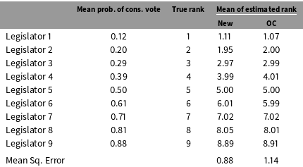
Table 1 shows the mean estimates and mean squared error based on the uniform bill distribution with 100 votes. Both the new estimator and the OC estimator recover the true rank of the ideal points quite well, although the new estimator has slightly lower mean squared error.

Table 1.

Estimate means for the uniform bill distribution.

Note: $N=100$ votes. Based on 10,000 Monte Carlo simulations. “New” indicates the estimator discussed in Section 3.

Table 2.

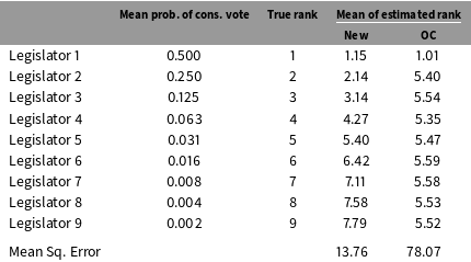
Estimate means for lopsided bill distributions.

Note: $N=100$ votes. Based on 10,000 Monte Carlo simulations. “New” indicates the estimator discussed in Section 3.

Table 2 shows the analogous results based on the lopsided bill distribution. Here, the legislators further to the right are all likely to vote together. Thus, it is difficult to estimate their relative positions. Both estimators do show higher mean squared error. However, while the new estimator and OC estimators performed relatively similarly with the uniform bill distribution, the new estimator performs significantly better here, with a mean squared error over 80% smaller.

Table 3.

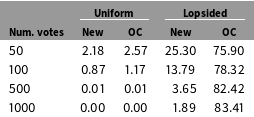
Mean squared error by number of votes

Finally, Table 3 shows mean squared error based on data with different numbers of votes. Again, using the uniform bill distribution, both models perform roughly similarly. However, for data generated using the lopsided bill distribution, the new estimator performs noticeably better. Further, whereas the mean squared error for the new estimator decreases as more votes are added, the mean squared error of OC appears to increase slightly as the number of votes increases.

5.2 Inference

To test the inference, I simulate data for two groups of bills, with vote probabilities for each generated from the uniform bill distribution. For the first simulation, the legislators maintain the same ordering on both sets of bills. Thus, the null hypothesis is true, so the test should not reject at the 5% significance level in more than 5% of simulations. Note that, given the weak assumptions underlying the test, it is likely to be conservative and reject in significantly less than 5% of simulations.

In the next simulation, I choose two neighboring legislators at random and swap their order, which provides as minimal a violation of the null hypothesis as possible. Only one pair of legislators is in a different order in one group of votes as in the other. All other pairs maintain the same ordering. Thus, the null hypothesis is false and can be correctly rejected, but, given that the change is relatively small, then it may be difficult to detect.

Finally, I simulate data in which the ordering of the legislators for the first group of bills is unrelated to the ordering for the second. Here, each possible ordering of the legislators is equally likely, with the ordering chosen for the first group of bills independent of the ordering chosen for the second.

Figure 1.

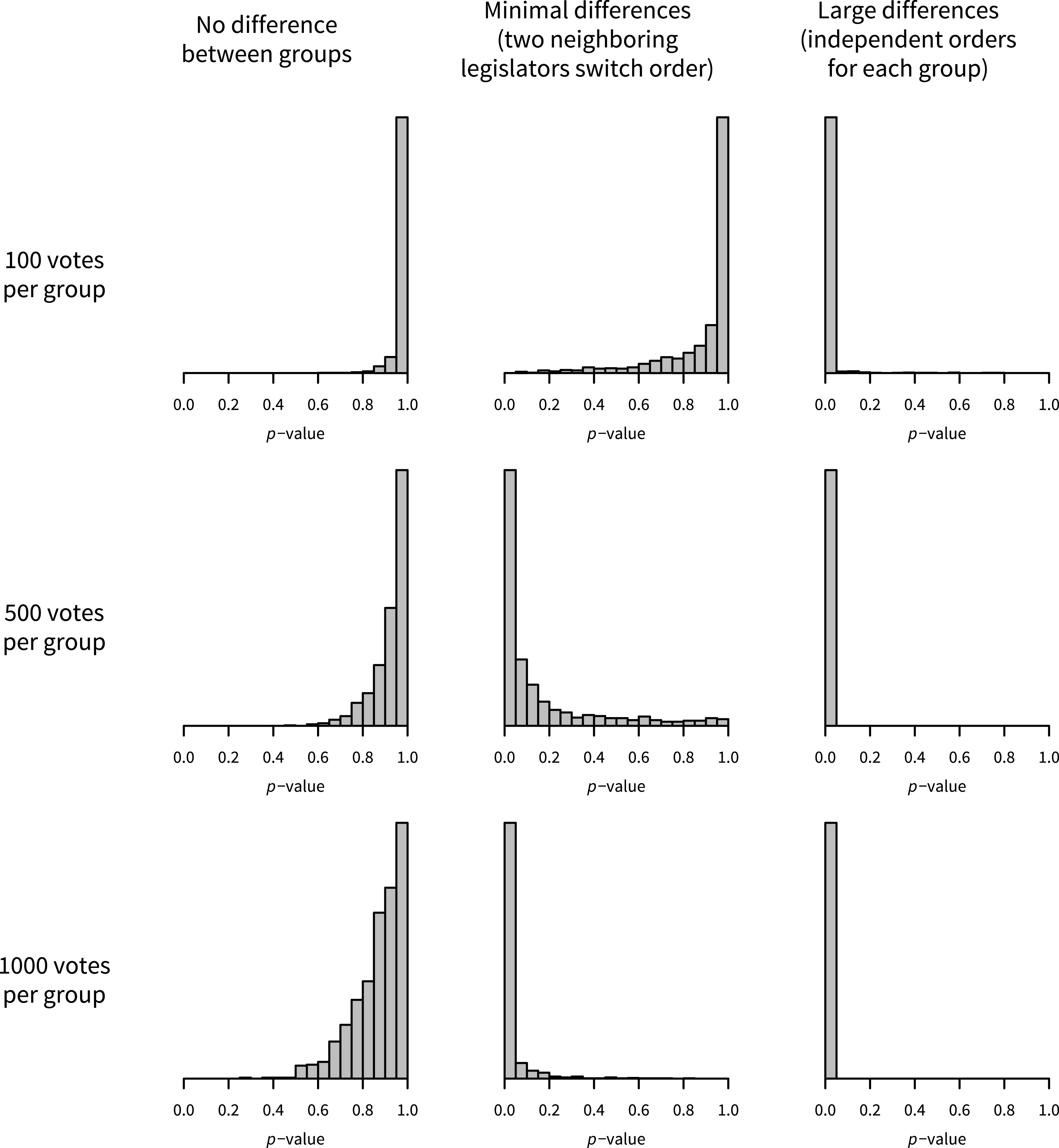
Histograms of p-values for test of same ordering from Monte Carlo simulations.

The results mirror expectations. Figure 1 shows histograms of p-values for each of the three scenarios discussed above and for each of 100, 500, and 1000 votes per group. The p-values in the first column, where the null hypothesis is true, tend to be greater than would be expected under a uniform distribution and the probability of rejection under the null hypothesis is below the nominal level of the test. This indicates the test is more conservative than possible, which is unsurprising.

In the second column, the null hypothesis is false but the orderings differ as little as possible. Here, the power of the test is quite low with 100 votes. However, as the number over voter increases, so does the power of the test. By 1000 votes, the probability of rejecting the null at the 5% significance level is 86.9%.

In the third column, the null hypothesis is false and a legislator’s ideology on one dimension is independent of her ideology on the other. Here, even with only 100 votes per group, the probability of rejecting the null is estimated to be 97.4%. With at least 500 votes per group, the power is over 99.9%.

6 Supreme Court

6.2 Is the Supreme Court multidimensional?

First, consider the question of whether the Supreme Court is multidimensional. Using data from the Supreme Court Database (Spaeth et al. Reference Spaeth, Epstein, Andrew D., Segal, Ruger and Benesh2015), I will use the hypothesis test developed in Section 4 to test whether a common dimension can explain voting on pairs of issue areas. I aggregate cases into four groups based on the Supreme Court Database’s coding of issue area: (1) criminal procedure, which includes only cases coded as “criminal procedure,” (2) civil liberties, which includes cases coded as “civil rights,” “First Amendment,” “due process,” and “privacy,” (3) economics, which includes cases coded as “economic activity,” “unions,” and “federal taxation,” and (4) other, which includes all other cases. Because the criminal procedure issue area is sometimes grouped together with the civil liberties issue areas and these issue areas are the ones “conventionally associated with the standard left–right splits on the Court” (Bailey Reference Bailey2013), I test whether a single ordering could explain voting on criminal procedure and civil liberties cases, treated as a single group, and on economics for each decade beginning with the 1950s.Footnote ¹⁵ I then similarly test whether a single ordering could explain voting on criminal procedure and economics, on civil liberties and economics, and on criminal procedure and civil liberties.

Table 4.

Tests of the hypothesis that the ideal points of Supreme Court justices are in the same order on cases on two different issue areas.

Note: Data from the Supreme Court Database (Spaeth et al. Reference Spaeth, Epstein, Andrew D., Segal, Ruger and Benesh2015). Civil liberties combines “civil rights,” “First Amendment,” “due process,” and “privacy” issue areas. Economics combines “economic activity,” “unions,” and “federal taxation” issue areas.

Table 4 shows the p-value computed for each comparison in each decade. Several comparisons are significant during the 1960s. Tests for the comparison between economics and criminal procedure, between economics and civil liberties, and between economics and both criminal procedure and civil liberties reject the null hypothesis that the ideal points have a common ordering during the 1960s at the 5% significance level. The test comparing criminal procedure and economics also nearly rejects for the 1970s ( $p=0.066$ ).

The p-values reported in the table make no adjustment for the fact that tests are performed for six different decades. However, even when the p-values for each comparison are adjusted using the Holm procedure so that the family wise error rate—that is, the collective probability of falsely rejecting the null across all six decades—for each comparison across all six decades is less than 5%, the null hypothesis can be rejected for the comparisons between economics and civil liberties (adjusted p-value of $0.039$ ) and between economics and both criminal procedure and civil liberties (adjusted p-value of $0.009$ ).Footnote ¹⁶

Thus, the extent to which the Court is multidimensional—that is, the extent to which different orderings are needed to explain Supreme Court voting on different issue areas—may depend on the time period in question. For the 1960s, we can reject the hypothesis that the justices had the same ordering on cases involving economics as on criminal procedure and civil liberties. On the other hand, there is no evidence that multiple dimensions are needed for other decades. Note that, while the number of cases the Court considered was slightly lower during the 1990s and 2000s, this alone does not appear to explain the difference, both because there were roughly equal numbers of cases considered for each issue area during the 1960s and 1980s and because the significance of the results persist for the 1960s even when using shorter, five-year periods of time.