1 Introduction
We study generic points for non-ergodic measures for certain non-statistical maps of the interval. Our results apply to a large class of interval maps admitting
$d \ge 2$
 equally sticky neutral fixed points. We first present our results in the context of a simple example. The full description will be given in §2.
Following [Reference Sera and YanoSY19], consider the transformation
$f \colon [0,1]\to [0,1]$
 given by

where
$c_1 = c_3 = 18$
 and
$c_2 = 72$
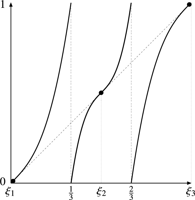
 , so that f is full-branched (see Figure 1). The map (1.1) has derivative
$f'(\cdot )> 1$
 , except at the neutral fixed points
$\xi _1 =0$
 ,
$\xi _2 = 1/2$
 , and
$\xi _3 =1$
 . This map admits a unique
$\sigma $
 -finite absolutely continuous ergodic invariant measure
$\mu $
 which gives infinite mass to the unit interval. (Unique up-to scaling by a positive constant.)
The map f given in (1.1).

Figure 1. Long description
The graph is set within a square frame. The vertical y-axis is labeled 0 at the bottom and 1 at the top with an upward arrow. The horizontal x-axis has labels xi sub 1 at the origin, 1 over 3, xi sub 2, 2 over 3, and xi sub 3 at the far right with a rightward arrow. A dashed diagonal line y equals x runs from the origin to the top-right corner.
There are three solid black curves representing the function f.
* The first curve starts at a solid black dot at the origin (xi sub 1, 0) and curves upward steeply, ending at the top edge of the square at x equals 1 over 3.
* The second curve starts at the x-axis at x equals 1 over 3 and curves upward, intersecting the dashed diagonal line at a solid black dot labeled xi sub 2. It continues upward to the top edge at x equals 2 over 3.
* The third curve starts at the x-axis at x equals 2 over 3 and curves upward to end at a solid black dot at the top-right corner (xi sub 3, 1).
Vertical dashed lines mark the boundaries at x equals 1 over 3, xi sub 2, and 2 over 3.
For
$x \in X$
 , let
$\delta _x$
 denote the Dirac delta measure at x. By [Reference Coates, Melbourne and TalebiCMT24], the map f given by (1.1) is non-statistical in the sense that for Lebesgue almost every x, the empirical measures

do not converge in the space of Borel probability measures in the weak
$\ast $
 topology, as
$n\to \infty $
 . Even more, for Lebesgue-almost every point x, these measures distribute along the simplex
$\pi {\mathcal S}$
 of invariant measures supported at the fixed points, where

and where
${\mathcal M}(f)$
 denotes the space of f-invariant Borel probability measures. Indeed, letting

by [Reference Coates, Melbourne and TalebiCMT24, Theorem A], one has

Given an f-invariant probability measure
$\nu $
 , consider its set of generic points or basin of attraction,

By [Reference Coates, Melbourne and TalebiCMT24], the basin of attraction of any measure in
$\pi {\mathcal S}$
 is negligible in terms of the Lebesgue measure

Moreover, by [Reference Pfister and SullivanPS07, Theorem 4.1] (see also (1.9)), it is also negligible in terms of the topological entropy (here, we use the concept of topological entropy
$h_{\text {top }}(f,\cdot )$
 on general (not necessarily compact) subsets following [Reference BowenBow74]) of f

Our main result, applied to the map (1.1), tells us that despite (1.5) and (1.6), these basins of attraction are in fact maximal in terms of Hausdorff dimension (we recall its definition in §6.5).
Theorem 1.1. For every
${\overline {p}} \in {\mathcal S}$
 ,
$ \dim _{\mathrm {H }} \mathscr {G} ( \nu _{\overline {p}} ) = 1. $

Note that the set
${\mathcal V}(x)$
 defined in (1.2) is a non-empty closed connected subset of
${\mathcal M}(f)$
 . Our second result tells us that for any closed connected subset of
$\pi {\mathcal S}$
 , the conclusion of the above theorem remains true.
Theorem 1.2. For every non-empty closed connected subset
${\mathcal C} \subset {\mathcal S}$
 ,
$ \dim _{\mathrm {H }} \{ x \colon {\mathcal V}(x) = \pi {\mathcal C} \} = 1. $

Theorems 1.1 and 1.2 fall within the scope of multifractal analysis, which investigates the ‘size’ of certain level sets of asymptotic quantifiers such as Birkhoff averages and local dimensions. In this type of analysis, two sorts of behavior are frequently studied: when a limit, say the average of a function
$\phi \colon X\to {\mathbb R}$
 , exists,

or when a limit does not exist, and the full range of irregular behavior with lower and upper limits
$\alpha <\beta $
 is investigated,

For a map f being a full shift and a function
$\phi $
 being Hölder continuous, the sets (1.7) and (1.8) can be characterized in terms of their Hausdorff dimension and topological entropy, and studied in terms of certain Gibbs measures which indeed govern the decay of deviations from the expected asymptotic average. See, for example, [Reference Barreira, Pesin and SchmelingBPS97] for references to some classical results.
The investigation of entropy of (1.7) and (1.8) is done in terms of certain rate functions that govern the decay of the distribution of Birkhoff averages over space. This type of analysis is also referred to as level-1 large deviation results (see [Reference EllisEll85, Reference YoungYou90] for details on rate functions and [Reference Takens and VerbitskiyTV03] for applications to multifractal analysis).
Here, we study level-2 deviations, focusing on empirical measures and their distributions. The study of divergence points, such as in (1.8), from the point of view of distributional measures (1.4) and quantification in terms of entropy, is given, for example, in [Reference Ercai, Küpper and LinEKL05]. In a similar spirit, for dynamical systems satisfying the specification property, [Reference Takens and VerbitskiyTV03] studies the entropy of Birkhoff averages-level sets, with a particular focus also on the Manneville–Pomeau map. As a precursor to [Reference Takens and VerbitskiyTV03, Reference Ercai, Küpper and LinEKL05], [Reference BowenBow74] showed that for a continuous map f on a compact metric space X, the entropy of f on the set of generic points (1.4) of an ergodic probability measure
$\nu $
 is

Non-generic points can also be described. By [Reference Pfister and SullivanPS07, Theorem 4.1] for any non-empty connected compact set
$\mathcal {C}\subset {\mathcal M}(f)$
 in the space of invariant Borel probability measures,

The equality in (1.9) also holds, but under stronger hypotheses, see [Reference Pfister and SullivanPS07]. In the setting of Theorem 1.1, one can show that (1.9) implies (1.6).
The study of Hausdorff dimension of level sets (1.7) and (1.8) usually requires some type of hyperbolicity as the results collected in [Reference Barreira, Pesin and SchmelingBPS97] illustrate. In [Reference Gelfert and RamsGR09, Reference Johansson, Jordan, Öberg and PollicottJJÖP10], the authors study non-uniformly hyperbolic interval maps with indifferent fixed points. These maps can be considered as on the boundary to hyperbolicity as they have the specification property and have a finite number of ergodic non-hyperbolic measures supported on parabolic fixed points. The studies in [Reference Gelfert and RamsGR09, Reference Johansson, Jordan, Öberg and PollicottJJÖP10] follow an approach of bridging measures based on ‘exhausting’ the non-uniformly hyperbolic part of dynamics by ‘uniformly hyperbolic sub-dynamics’, see also [Reference Barreira and SchmelingBS00]. Theorems 1.1 and 1.2 focus on empirical measures and the non-hyperbolic part. The approach in [Reference Gelfert and RamsGR09] will also be a key step to prove the assertion about the dimension of (1.4) in Theorem 1.1.
The phenomenon (1.3) for a map with just two parabolic fixed points was shown in [Reference Aaronson, Thaler and ZweimüllerATZ05, Reference Coates and LuzzattoCL24, Reference Barrientos and ChavezBC24] and in [Reference Coates, Melbourne and TalebiCMT24] for maps with several parabolic fixed points. More generally, non-statistical behavior was observed in other contexts. For example, in the quadratic family, Hofbauer and Keller [Reference Hofbauer and KellerHK95] prove that there are uncountably many parameters which correspond to a map f which has ‘maximal oscillation’ in the sense that for Lebesgue almost-every initial condition, the empirical measures accumulate on the full simplex of f-invariant Borel probability measures. In [Reference TalebiTal22], the maximal oscillation-property was shown to hold generically for a certain class of rational maps. Finally, [Reference Andersson and GuihéneufAG22] establishes an analogous version of (1.3) for certain irrational linear flows of the two-torus (see also the references therein for further results in this direction).
The paper is organized as follows. In §2, we introduce the more general setting which we study (for which (1.1) is a particular example) and state our main result, Theorem A. Theorems 1.1 and 1.2 are special cases of Theorem A. Section 4 provides details on repellers and return times. In §§3, 5, and 6, we prove Theorem A. In §8, we provide further examples to which Theorem A applies.
2 Assumptions and statement of results
2.1 Assumptions
We recall some classical definitions and make precise the assumptions we use throughout the paper. Throughout, we let X denote either the circle
$\mathbb {S}^1$
 or the interval
$[0,1]$
 . We say that a non-singular transformation
$f\colon X\to X$
 is Markov if there exists a countable partition (modulo
$\mathrm {Leb}$
 )
${\mathcal P}$
 of X into closed sub-intervals such that the restriction of f to any partition element is a bijection onto a union of partition elements. A Markov map f with partition
${\mathcal P}$
 is topologically mixing if for every
$a,b \in {\mathcal P}$
 , there exists an
$N\in {\mathbb N}$
 such that
$f^n (a) \cap b \neq \emptyset $
 for every
$n \geq N$
 .
Assumption 2.1. Assume
$f\colon X \to X$
 is a Markov map with respect to a partition
${\mathcal P}$
 .
Assumption 2.2. There exists a union of partition elements Y so that the first return map
$F\colon Y \to Y$
 given by

where

is a topologically mixing
$C^2$
 uniformly expanding Gibbs–Markov map with respect to a refinement
${\mathcal Q}$
 of
${\mathcal P}$
 . That is, F is Markov with respect to
${\mathcal Q}$
 , topologically mixing, and the following additional properties hold.
-
• (Finite images) $\mathrm {Card} \{ F (a) \colon a \in {\mathcal Q} \} < \infty $
 , that is, there exist
$Y_1,\ldots , Y_L$
so that each
$Y_i$
is a union of elements of
${\mathcal Q}$
and
$\{F(a)\colon a\in {\mathcal Q}\} = \{ Y_1, \ldots , Y_L\}$
.
-
• (Bounded distortion) There exist $\theta \in (0,1)$
and
$C> 0$
so that the function
$\log ({d m}/{dm \circ F})$
is
$d_\theta $
-Lipschitz on elements of
${\mathcal Q}$
, where
$d_{\theta }$
is the metric and -
• ( $C^{ 2 }$
branches) For every
$a\in {\mathcal Q}$
, the map
$F|_{\mathrm {int}(a)}\colon \mathrm {int}(a) \to F(\mathrm {int}(a))$
is a
$C^{ 2 }$
diffeomorphism. (Notice that we do not necessarily assume that F has
$C^{ 2 }$
extension to the closure of a.) -
• (Uniform expansion) There exists $\unicode{x3bb}> 1$
such that
$\inf _{ x\in Y} |F'(x)|> \unicode{x3bb} $
.









 and






Lemma 2.3. Up to taking a possible refinement of the partition
${\mathcal Q}$
 , we may assume that
$F({\mathcal Q}) = \{ Y_1, \ldots , Y_n \}$
 is a collection of disjoint subintervals which partition Y.
Proof. Let
$\{ y_1 < y_2 \cdots < y_{N - 1} < y_{N}\}$
 be the collection of end points of the intervals
$Y_i$
 ordered so that
$y_i < y_{i + 1}$
 and let
${\mathcal Y}$
 denote the partition of Y given by all intervals of the form
$[y_{i}, y_{ i + 1 }]$
 that intersect Y. As each
$Y_i$
 is a union of elements of
${\mathcal P}$
 , it follows that each element in
${\mathcal Y}$
 is also a union of elements of
${\mathcal P}$
 .
As each
$Y_i$
 is a finite union of elements in
${\mathcal Y}$
 , f is a bijection on elements of
${\mathcal P}$
 and we can refine
${\mathcal P}$
 to form a new partition
$\widetilde {{\mathcal Q}}$
 so that
$f(a) \in {\mathcal Y}$
 for all
$a\in \widetilde {{\mathcal Q}}$
 .
Remark 2.4. Up to taking a refinement of
${\mathcal Q}$
 , we can assume that
$\tau $
 takes a finite and constant value on the interior of every
$a\in {\mathcal Q}$
 .
Remark 2.5. As the first return map F is Gibbs–Markov, it preserves an invariant probability measure
$\mu _Y$
 which is equivalent to Lebesgue (see, for example, [Reference AaronsonAar97, Ch. 4]). This implies that f preserves the
$\sigma $
 -finite f-invariant ergodic measure
$\mu $
 equivalent to Lebesgue given by

Defining
$\mu $
 in this way, one notes that
$\mu |_Y = \mu _Y$
 (if
$A \subset Y$
 , then one has that
$\{ \tau> n \} \cap f^{-n}) A = \emptyset $
 for every
$n \ge 1$
 as
$Y \cap f^{-n} A \subset \{ \tau \le n \}$
 ) and that

Notice that in our definition of Gibbs–Markov in Assumption 2.2, we assume the finite image property instead of the slightly weaker ‘big image property’ which also commonly appears in the literature (see, for example, [Reference ZweimüllerZwe98, Reference ZweimüllerZwe00, Reference GouëzelGou10]). This stronger assumption guarantees that
$\mu _Y$
 , and hence
$\mu $
 , is equivalent to Lebesgue as opposed to only being absolutely continuous with respect to Lebesgue.
Assumption 2.6. There exist constants
$d \in {\mathbb N}$
 ,
$\alpha \in (0,1)$
 , and
$\gamma _1, \ldots , \gamma _d>0$
 , and a partition (mod
$\mathrm {Leb}$
 ) of
$X \setminus Y$
 into open sets
$X_1,\ldots ,X_d$
 such that for every
$i,j\in \{1,\ldots ,d\}$
 :
-
(1) there is a single fixed point $\xi _j \in X_j$
; -
(2) for $i \neq j$
, orbits cannot pass from
$X_i$
to
$X_j$
without first passing through Y, that is, if
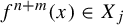
$f^{ n } (x) \in X_{ i }$
and
$f^{ n + m }(x) \in X_{ j }$
for some
$i \neq j$
and
$m\in {\mathbb N}$
, then there is
$k \in \{1,\ldots ,m-1\}$
such that
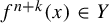
$f^{ n+k }( x) \in Y$
, -
(3) $\mu _Y ( \tau ^{(j)}> n ) \sim \gamma _j n^{-\alpha }$
, where







Remark 2.7. Notice that each connected component of  is the preimage of an interval (a connected component of Y) by one of the branches of f (a
$C^2$
 diffeomorphism). Thus, the sets
$J_n$
 necessarily accumulate at fixed points of f, in the sense that

Remark 2.8. Item (2) in Assumption 2.6 tells us that for any
$x \in Y$
 , only one of the values
$\tau ^{(1)} (x), \ldots , \tau ^{(d)}(x)$
 can be non-zero. In particular,

and so

In particular,
$\int \tau \, d\mu _Y = \infty $
 and so
$\mu ( X ) = \infty $
 .
2.2 Statement of results
Throughout the remainder of the article, we assume that f is a map satisfying Assumptions 2.1–2.6. Compare also Figure 2. We consider

Denoting by  the nth empirical measure of
$x \in X$
 , we consider

of weak
$\ast $
 limit points of the empirical measures. The following is our main result.
Theorem A. If Assumptions 2.1–2.6 hold, then for every closed connected set
${\mathcal C}\subset {\mathcal S}$
 ,

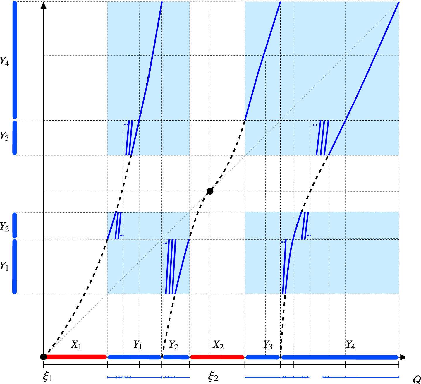
An example of a Markov map
$f\colon [0,1]\to [0,1]$
 (dashed curve) with two parabolic fixed points
$\xi _1,\xi _2$
 and its Gibbs–Markov first return map
$F\colon Y\to Y$
 (solid curve) on the set Y (union of intervals
$Y_1,\ldots,Y_4$
 ). See Example 8.3. The collection
$\{Y_1,\ldots ,Y_4\}$
 of sets
$\{F(a)\colon a\in {\mathcal Q}\}$
 cover Y, see Assumption 2.2. (Color online.).

Figure 2. Long description
The graph is plotted on a square domain from 0 to 1 on both axes.
- Horizontal Axis: Labeled with intervals X sub 1 (red), Y sub 1 (blue), Y sub 2 (blue), X sub 2 (red), Y sub 3 (blue), and Y sub 4 (blue). Two fixed points are marked: xi sub 1 at the origin and xi sub 2 near the center. A secondary axis below labeled Q shows a Cantor-like set structure.
- Vertical Axis: Labeled with blue vertical bars corresponding to intervals Y sub 1, Y sub 2, Y sub 3, and Y sub 4.
- Curves: A dashed black curve represents the Markov map f, which passes through the origin and xi sub 2. A solid blue curve represents the first return map F, consisting of several steep branches that span the height of the shaded blue regions.
- Shaded Regions: Four light blue rectangular zones are positioned where the x-intervals Y sub 1 through Y sub 4 intersect with the y-intervals Y sub 1 through Y sub 4.
- Geometric Features: A diagonal dotted line y equals x serves as a reference. The solid blue branches of F are restricted to the x-intervals Y sub 1, Y sub 2, Y sub 3, and Y sub 4, showing a piecewise monotonic increase within each interval.
Considering the special case that
${\mathcal C} = \{ {\overline {p}} \}$
 , one obtains the following corollary.
Corollary 2.9. If Assumptions 2.1–2.6 hold, then
$\dim _{\mathrm {H }} \mathscr {G} ( \nu _{{\overline {p}}} ) = 1$
 for every
${\overline {p}} \in {\mathcal S}$
 .
Remark 2.10. We only treat the case that
$\alpha \in (0,1)$
 even though the case
$\alpha = 1$
 is also known to lead to non-statistical behavior [Reference Coates, Melbourne and TalebiCMT24]. Our method of proof will rely heavily on knowing that occupation times of neighborhoods of the fixed points converge in distribution to a non-degenerate limit. For
$\alpha \in (0,1]$
 , it is known that in our present setting, these occupation times will converge in distribution to a generalized arcsine law (cf. [Reference Sera and YanoSY19, Reference SeraSer20] and Lemma 5.3 for a precise statement). However, when
$\alpha = 1$
 , this arcsine law is degenerate and our methods break down.
One can also consider the case
$\alpha = 0$
 , which corresponds to the map making flat tangencies at the neutral fixed points (that is, the derivative at the fixed points converge to
$1$
 exponentially fast). In this case, the tails of the return time
$\mu _Y ( \tau> n )$
 decay logarithmically [Reference DesaiDes23] and our methods (which rely heavily on
$\mu _Y ( \tau> n )$
 decaying polynomially) break down.
Sections 3–7 are devoted to proving Theorem A. It will be convenient to first prove Corollary 2.9, which is a special case.
The first key step is to establish a coding of generic points in terms of the asymptotic behavior of their return times. For this, we will consider the joint behavior of the return times
$\tau ^{(1)},\ldots ,\tau ^{(d)}$
 and their Birkhoff sums under F. To this end, we introduce

and let

and define the
$\tau ^{(i)}_k$
 analogously for
$i=1,\ldots ,d$
 . In §3, we will show

Equation (2.3) reduces the problem of understanding the observables
$e_n\colon X \to {\mathcal M}(f)$
 under the dynamics of f to understanding the Birkhoff sums of the function
${\overline {\tau }} \colon Y \to {\mathbb N}^d$
 under the dynamics of a uniformly expanding Gibbs–Markov map F.
By Remark 2.4,
${\overline {\tau }}$
 is piecewise constant. So, together with (2.3), we obtain a symbolic description of
$\mathscr {G} (\nu _{{\overline {p}}})$
 (albeit one that requires an infinite alphabet) and can start building approximations of
$\mathscr {G} ( \nu _{{\overline {p}}} )$
 . Namely, we will construct collections
${\mathcal A}$
 of cylinder sets where the return times have a certain prescribed behavior up to some finite time. This will be done in such a way that: the limit points of
$({\overline {\tau }}_k/\tau _k)_k$
 will all be close to
${\overline {p}}$
 for points in the maximal invariant set of
${\mathcal A}$
 ; and the dimension of this maximal invariant set is close to
$1$
 . See §§4 and 5.
In §6, we then consider a sequence
$({\mathcal A}_i)_i$
 of increasingly better approximations to
$\mathscr {G}(\nu _{\overline {p}})$
 to build a set
$\Gamma \subset \mathscr {G} ( \nu _{\overline {p}} )$
 . We conclude by arguing that
$\dim _{\mathrm {H}} \Gamma = 1$
 .
Finally, in §7, we explain how the proof of Corollary 2.9 can be strengthened to prove Theorem A.
3 Coding of
$\nu _{\bar p}$
-generic points

In this section, we explore equivalent characterizations of the convergence of the empirical measures in terms of the return times
${\overline {\tau }}$
 by relating
${\mathcal V}(x)$
 and the set

Theorem 3.1. Let be
${\mathcal T}(x)$
 a closed connected subset of
${\mathcal S}$
 and suppose that

Then,
${\mathcal V}(x) = \pi ({\mathcal T}(x) )$
 .
The above theorem will be proven at the end of this section. When
${\mathcal C}$
 contains a single point
${\overline {p}}$
 , Theorem 3.1 reduces to the following result.
Corollary 3.2. For all
$x\in X$
 and
${\overline {p}} \in {\mathcal S}$
 ,

We begin with the following intermediate result.
Proposition 3.3. If
$\mathcal {T}(x) \subset {\mathcal S}$
 , then
${\mathcal V}(x) \subset \pi {\mathcal S}$
 .
To prove Proposition 3.3, we first collect some preliminary results. From the ergodic theorem for infinite measures, we know that

holds for Lebesgue-almost every x. (The ergodic theorem (see [Reference AaronsonAar97, Exercise 2.2.1]) here tells us that
$e_n(x)(A) \to 0$
 for
$\mu $
 -almost every x and for all A with
$\mu (A) < +\infty $
 . The fact that any compact set which does not contain any of the neutral fixed points has finite measure is an easy consequence of Remark 2.7 and (2.1).) Recall that
$e_n(x)(K)$
 is just the proportion of time up to time n that the orbit of x spends in K. So, if (3.2) holds for some x, then its orbit must spend proportion
$1$
 of its time near the fixed points. This, in turn, suggests
${\mathcal V}(x) \subset \pi {\mathcal S}$
 . Indeed, we get the following result.
Lemma 3.4. For any
$x\in X$
 ,
${\mathcal V}(x) \subset \pi {\mathcal S}$
 and (3.2) are equivalent.
Proof. The Portmanteau theorem tells us that
${\mathcal V}(x) \subset \pi {\mathcal S}$
 if and only if the only limit point of
$(e_n(x)(A))_n$
 is
$0$
 whenever
$A\subset X$
 is such that
$ \partial A \cap \{ \xi _1 , \ldots , \xi _d\} = \emptyset $
 . The result quickly follows.
From our discussion above, it is now clear that
${\mathcal V}(x) \subset \pi {\mathcal S}$
 for Lebesgue-almost every x. (Indeed, note that by [Reference Coates, Melbourne and TalebiCMT24], the reverse inclusion
$\pi \mathcal {S}\subset \mathcal {V}(x)$
 also holds for Lebesgue-typical x). We are interested, though, in the behavior of non-typical points. Moreover, we want to encode condition (3.2) using the symbolic dynamics of the induced map. For that, we introduce the condition


Proof. Assume (3.2). Notice that

Hence, (3.3) follows immediately from (3.2) by taking
$K = Y$
 .
Now, assume (3.3). As
$K \subset X$
 is a compact set which does not contain any of the neutral fixed points, we know from Remark 2.7 that
$\sup _{ K \setminus Y } \tau < \infty $
 . Setting

the number of entrances to K between successive returns to Y is at most N, that is,

For each
$n \in {\mathbb N}$
 , choose
$k_{ n } \in {\mathbb N}$
 such that

By the definition of
$k_{ n }$
 and N, we have

by our assumption on x. This proves (3.2).
Proof of Proposition 3.3
By Lemmas 3.4 and 3.5, it is enough to show that
${\mathcal T}(x) \subset {\mathcal S}$
 implies (3.3). We first claim that

From (2.2), we know that
$\sum _{ j = 1 }^{d} \tau _k^{(j)}(x) / \tau _k (x) \le 1$
 . So, the sequence in the limit in (3.4) is bounded and, hence, we can choose a subsequence
$(k_\ell )_\ell $
 so that

for some
$c \in [0,d]$
 . By the compactness of
$[0,1]^d$
 , up to passing to a further subsequence, we can assume that
$\lim _{\ell \to \infty } ( {\overline {\tau }}_{ k_\ell }/ \tau _{k_\ell } ) (x) = (p_1,\ldots ,p_d)$
 . However, as all the limit points
${\mathcal T} (x)$
 of
$(({\overline {\tau }}_k/\tau _k)(x))_k$
 are contained in
${\mathcal S}$
 , we find that

which proves (3.4).
Now, using (2.2), we see that

Define

Lemma 3.6. If
${\mathcal V}(x) \subset \pi {\mathcal S}$
 , then
${\mathcal V}(x) = \pi ( \widetilde {\mathcal T}(x) )$
 .
Proof. Suppose that
${\mathcal V}(x) \subset \pi {\mathcal S}$
 .
As the observable  is continuous at the continuity points of any measure in
$\pi {\mathcal S}$
 , the Portmanteau theorem tells us that if
$e_{n_k}(x) \to \nu _{\overline {p}}$
 for a subsequence
$(n_k)_k$
 and some
${\overline {p}} \in {\mathcal S}$
 , then

Thus,
${\mathcal V}(x) \subset \pi \widetilde {\mathcal T}(x)$
 .
Now, suppose that
$\lim _{k\to \infty }(e_{n_{k}}(x) (X_1), \ldots , e_{n_k}(x)(X_d)) = {\overline {p}}$
 for a subsequence
$(n_k)_k$
 . Reasoning as in (3.5), we see that the only possible limit point of
$(e_{n_k}(x))_k$
 is
$\nu _{\overline {p}}$
 . By compactness,
$\lim _{k \to \infty }e_{n_k}(x) = \nu _{\overline {p}}$
 , which gives
$\widetilde {{\mathcal T}}(x) \subset \pi ^{-1}{\mathcal V}(x)$
 .
Proof of Theorem 3.1
Suppose that
${\mathcal T}(x)$
 is a closed connected subset of
${\mathcal S}$
 . By Proposition 3.3,
${\mathcal V}(x) \subset \pi {\mathcal S}$
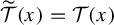
 . Thus, from Lemma 3.6, it is enough to show that
$\widetilde {\mathcal T}(x) = {\mathcal T}(x)$
 . As

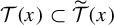
it is clear that
${\mathcal T}(x) \subset \widetilde {{\mathcal T}}(x)$
 .
By Assumption 2.6(2), the orbit of x spends all of its time in at most one of the sets
$X_{ 1 }, \ldots , X_{ d }$
 between any two successive entrances to Y. Thus, for any given
$j = 1,\ldots , d$
 ,
$k \in {\mathbb N}$
 , and
$0 \le \ell < \tau _{k + 1} (x) - \tau _k(x)$
 , one has for
$n = \tau _k(x) + \ell $
 that either

and the former is increasing in
$\ell $
 and the latter is decreasing in
$\ell $
 . (Notice that the derivative of
$t \mapsto ({ a + t }/{ b + t })$
 is
$({ b - a }/{ ( b + t )^{ 2 }})$
 , which is non-negative whenever
$b \ge a$
 .) Thus, the sequence
$(e_n(X_j))_n$
 is strictly monotonic on each time interval
$[\tau _{k}(x), \tau _{k+1}(x)] \cap {\mathbb N}$
 . This tells us that

Suppose that (3.1) is satisfied and let

Hence, as
${\mathcal T}(x)$
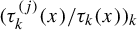
 are the limit points of
$(\tau _k^{(j)}(x)/\tau _k(x))_k$
 , for all k sufficiently large, we get

Thus, we get that

which implies that
$\widetilde {\mathcal T}(x)\subset {\mathcal T}(x)$
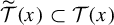 . This concludes the proof.
4 Auxiliary results on repellers and return times
In this section, we collect some auxiliary results on ‘sub-repellers’ for some (high enough) iterate
$F^n$
 of our initial map F.
4.1 Cylinders and associated maximal invariant sets
Given
$n\in {\mathbb N}$
 , we let

denote the refinement of
${\mathcal Q}$
 under F into n-cylinders. Write

for the collection of all cylinders. Given
$a \in {\mathcal Q}^{n}$
 and
$b\in {\mathcal Q}^{*}$
 , we write
 .
We denote by
$|a|$
 the length of the interval
$a\in {\mathcal Q}^\ast $
 .
Unless there is a risk of misunderstanding, given a collection of n-cylinders
${\mathcal A} \subset {\mathcal Q}^n$
 , we use the symbol
${\mathcal A}$
 also to denote the union of all partition elements that
${\mathcal A}$
 contains. For
${\mathcal A} \subset {\mathcal Q}^n$
 , consider the associated maximal invariant set

Given any
$A \subset X$
 , we denote by
${\mathcal Q}_{A}^\ell $
 the set of
$\ell $
 -cylinders whose interiors intersect A,

Remark 4.1. Notice that if
${\mathcal A} \subset {\mathcal Q}^n$
 , then for every
$k\in {\mathbb N}_0$
 and
$s\in \{0,\ldots , n - 1\}$
 ,

4.2 Geometric properties of repellers formed from maximal invariant sets
Given a finite collection
${\mathcal A} \subset {\mathcal Q}^n$
 , we define the virtual dimension
$\mathrm {vdim} \,\Lambda ( {\mathcal A} ) $
 of its maximal invariant set
$\Lambda ( {\mathcal A} )$
 defined in (4.1) by setting

By Assumption 2.2, the map F is a
$C^{ 2 }$
 uniformly expanding Markov map with bounded distortion. Hence, there exist a
$\unicode{x3bb}> 1$
 and a constant
$D> 0$
 such that for every
$n\in {\mathbb N}$
 ,

In particular, map
$g = F^n|_{\Lambda ({\mathcal A} )}$
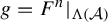 is an expanding repeller in the sense of [Reference Przytycki and UrbańskiPU10]. That is, equipping Y with the topology induced by the separation time distance,
$\Lambda ({\mathcal A})$
 is a repeller for g:
-
• $g(\Lambda ({\mathcal A})) = \Lambda ( {\mathcal A} )$
; -
• $g|_{{\mathcal A}}$
is continuous; -
• ${\mathcal A} \subset Y$
is open and
$\Lambda ( {\mathcal A} ) = \bigcap _{ k = 0 }^{ \infty } g^{-k} {\mathcal A}$
; and -
• g is expanding: $|(g^k)'(x)| \ge \unicode{x3bb} ^{nk}$
for all
$x\in \Lambda ( {\mathcal A})$
.






Remark 4.2. Estimates (4.3) imply that

and

From [Reference Palis and TakensPT93, proof of Theorem 3, §4.2], we then obtain the following lemma.
Lemma 4.3. Let
${\mathcal A} \subset {\mathcal Q}^n$
 be a finite subcollection. If
$F^n\colon \Lambda ( {\mathcal A} ) \to \Lambda ( {\mathcal A} )$
 is topologically mixing, then

where
$D> 0$
 and
$\unicode{x3bb}> 1$
 are as in (4.3).
A Borel probability measure m is geometric for
$F^n|_{\Lambda ( {\mathcal A})}$
 if it is ergodic and invariant for
$F^n$
 ,
$m ( \Lambda ( {\mathcal A} ) )= 1$
 , and if there exists a constant
$E> 0$
 so that

for all
$x \in \Lambda ( {\mathcal A} )$
 and all
$r> 0$
 . The following is provided, for example, by [Reference Przytycki and UrbańskiPU10, Theorem 9.1.6] and [Reference Przytycki and UrbańskiPU10, Theorem 8.1.6], by taking m to be the Gibbs state corresponding to the function
$-d\log |(F^n)'|$
 (with respect to the mixing expanding repeller
$F^n|_{\Lambda ({\mathcal A})}$
 ), with
$d= \dim _{\mathrm {H}}\Lambda ({\mathcal A})$
 .
Lemma 4.4. For any
${\mathcal A}\subset {\mathcal Q}^n$
 so that
$F^n|_{ \Lambda ({\mathcal A})}$
 is topologically mixing, there exists a corresponding geometric measure m.
4.3 Return times on cylinders
By Remark 2.4, the function
$\tau $
 (and, hence, the vector-valued function
${\overline {\tau }}$
 ) is constant on the interior of each element of
${\mathcal Q}$
 . Thus, for any
$n\in {\mathbb N}$
 , the value of
${\overline {\tau }}_{ n }(x)$
 is completely determined by the n-cylinder which contains x. For
$a\in {\mathcal Q}^{ n }$
 , we will thus write
${\overline {\tau }}_{ n }(a)$
 for the value of
${\overline {\tau }}_{ n }|_{ \mathrm {int}(a) }$
 .
Remark 4.5. For
$x,y,v,w>0$
 ,

For
$\overline {x}, \overline {y} \in {\mathbb R}^{ d }$
 , and
$v,w \neq 0$
 , we have that

From Remark 4.5, we obtain the following simple inequalities. Here, all equalities involving vectors in
${\mathbb R}^d$
 are to be understood coordinate-wise. For
$\overline {x} \in {\mathbb R}^d$
 , let
 .
Lemma 4.6. For every
$a \in {\mathcal Q}^n$
 and
$b \in {\mathcal Q}^k$
 such that
$ab\in {\mathcal Q}^{n+k}$
 :
-
(1) $|({{\overline {\tau }}_{ n + k }}/{\tau _{ n + k}})(ab)- ({{\overline {\tau }}_n}/{\tau _n}) (a)| \leq ({2 \tau _k (b)})/({\tau _{n} (a) + \tau _k (b)})$
; -
(2) $|({{\overline {\tau }}_{ n + k}}/{\tau _{ n + k}})(ab) - ({{\overline {\tau }}_k}/{\tau _k}) (b)| \leq ({2 \tau _n (a)})/({\tau _{n}(a) + \tau _k (b)})$
; -
(3) $\min \{({{\overline {\tau }}_{n}}/{\tau _{n}}) (a), ({{\overline {\tau }}_{k}}/{\tau _{k}}) (b)\} \le ({{\overline {\tau }}_{n + k}}/{\tau _{n + k}}) (ab)\leq \max \{({{\overline {\tau }}_{n}}/{\tau _{ n }}) (a), ({{\overline {\tau }}_{k}}/{\tau _{k}}) (b)\}$
.



Proof. First, notice that

The inequality in item (3) then follows from (4.7). Also note that
$|{\overline {\tau }}_j/\tau _{ j }| \le 1$
 . Hence, (4.8) implies

together with the analogous lower bound. This proves item (1). The proof of item (2) is analogous.
5 Approximation by repellers
Recall the big image property for F from Assumption 2.2 stating that  for some
$L\in {\mathbb N}$
 . It hence follows that

In this section, we will prove the following proposition.
Proposition 5.1. For every
${\overline {p}} \in {\mathcal S}$
 and every
$\varepsilon> 0$
 , there exist
$n,N \in {\mathbb N}$
 , a finite subset
${\mathcal A} \subset {\mathcal Q}^n$
 , and a Borel probability measure m on Y such that: the image of
${\mathcal A}$
 under
$F^n$
 covers Y and, in particular,
$F^n ( {\mathcal A} ) = {\mathcal Y}$
 ;
$m(\Lambda ({\mathcal A})) = 1$
 ; and
$m ( \Lambda ({\mathcal A}) \cap Y_i )> 0$
 for each
$i = 1, \ldots , L$
 . Moreover,

Throughout this section, we fix
${\overline {p}}\in {\mathcal S}$
 and
$\varepsilon \in (0,1)$
 . In §5.1, we construct, for each
$n \in {\mathbb N}$
 sufficiently large, a collection of n-cylinders
${\mathcal A}(n)$
 . In §§5.2 and 5.3, we show, for all
$\ell \in {\mathbb N}$
 sufficiently large, that cylinders
$a \in {\mathcal Q}_{\Lambda ({\mathcal A}(n))}^{\ell }$
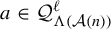 satisfy the assertion (5.2) of Proposition 5.1 with respect to a certain measure
$m(n)$
 on
$\Lambda ({\mathcal A}(n))$
 .
5.1 Construction of
${\mathcal A}(n)$

Proposition 5.2. There exists
$C\in (0,1)$
 so that for every n sufficiently large, there is a finite collection
${\mathcal A}(n) \subset {\mathcal Q}^{ n }$
 such that:
-
(1) ${\mathcal A}(n) \subset \{ a \in {\mathcal Q}^n \colon {\overline {\tau }}_{ n } (a) / \tau _{ n } (a) \in B_{ 3\varepsilon /4 } ( {\overline {p}} ) \}$
; -
(2) $\mathrm {Leb} ({\mathcal A} (n) \cap Y_i)> C$
for all
$i = 1, \ldots , L$
; -
(3) $F^{ n } {\mathcal A}(n) = {\mathcal Y}$
.




We divide the proof of Proposition 5.2 into several intermediate lemmas. First, we give the following uniform lower bound for the Lebesgue measure of the set of points x where the ratio
$({\overline {\tau }}_{ n } / \tau _{ n }) (x)$
 is close to
${\overline {p}}$
 .
Lemma 5.3. There exists
$C^{\prime }> 0$
 such that

for all n sufficiently large.
Proof. Let us first prove that there exists a random variable
$\boldsymbol {Z}$
 whose distribution
$\boldsymbol Z_{ * } {\mathbb P}$
 on
${\mathcal S}$
 is equivalent to
$\mathrm {Leb}$
 and such that the random variables

converge in distribution to
$\boldsymbol {Z}$
 as
$n\to \infty $
 , that is,

This follows from [Reference SeraSer20, Corollary 4.2 and Theorem 3.3], provided one can check [Reference SeraSer20, Assumptions 2.1, 2.2, and 2.6]. Assumption 2.6 yields [Reference SeraSer20, Assumption 2.1], and then Assumption 2.6(3) together with [Reference SeraSer20, Lemma 2.4] gives [Reference SeraSer20, Assumption 2.2]. Finally, as
$F $
 is topologically mixing, it is exponentially continued fraction mixing (see, for example, [Reference AaronsonAar97, §4]), which yields [Reference SeraSer20, Assumption 2.6].
Recall that, as in the proof of Theorem 3.1, we have that for all
$x\in X$
 ,

Thus, as the distribution of
$\boldsymbol Z_\ast {\mathbb P}$
 of
$\boldsymbol Z$
 is equivalent to Lebesgue on
${\mathcal S}$
 , we can take
$A = B_{\varepsilon / 2 } ( {\overline {p}} )$
 in the above to obtain

This implies the conclusion of the lemma for the measure
$\mu $
 . Finally, as (see Remark 2.5)
$\mu $
 is equivalent to
$\mathrm {Leb}$
 , this implies the assertion.
Lemma 5.4. There is
$k_0 \in {\mathbb N}$
 such that for every
$i,j\in \{1,\ldots ,L\}$
 , there exists
$a_{ij}\subset Y_i$
 such that
$a_{ij}\in {\mathcal Q}^{k_0}$
 and
$F^{k_0}(a_{ij})=Y_j$
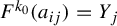 .
Proof. Fix
$i,j \in \{ 1, \ldots , L \}$
 and fix
$a_i \in {\mathcal Q}$
 with
$a_i \subset Y_i$
 . As F is topologically mixing, we can choose
$k_{ij} \in {\mathbb N}$
 to be such that, for all
$n \ge k_{ij}$
 ,

Let  . Hence, there is
$a_{ij} \in {\mathcal Q}^{k_0} \cap a_i$
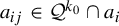 such that
$F^{k_0}( a_{ij}) \cap Y_j \neq \emptyset $
 . However, we know that
$F^{k_0}( a_{ij}) \in \{ Y_1, \ldots , Y_L \}$
 , Hence, we get
$F^{k_0}(a_{ij}) = Y_j$
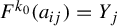 .
Proof of Proposition 5.2
Given
$n \in {\mathbb N}$
 , let

and let
${\mathcal B}(n)^\prime \subset {\mathcal B}(n)$
 be a finite sub-collection so that
$\mathrm {Leb} ( {\mathcal B}(n)^\prime ) \ge \tfrac 12 \mathrm {Leb}( {\mathcal B}(n) )$
 . Thus, by Lemma 5.3, there exists some constant
$C^\prime> 0$
 so that

Let
$k_0$
 and
$\{ a_{ij} \}_{i,j = 1}^{L}$
 be as given by Lemma 5.4. As F is assumed to be a topologically mixing Gibbs–Markov map, each element of
${\mathcal Y}$
 is a union of elements of
${\mathcal Q}$
 , and the union of all elements in
${\mathcal Y}$
 equals Y. So, for any cylinder
$b \in {\mathcal Q}^n$
 , we know from (5.1) that there exist
$p(b),s(b) \in \{ 1, \ldots , L\}$
 so that
$b \subset Y_{p(b)}$
 and
$F^n (b) = Y_{s(b)}$
 . Thus, for all
$i,j\in \{1,\ldots , L\}$
 , the cylinder
$a_{i p(b)} b a_{s(b) j} \in {\mathcal Q}^{n + 2 k_0}$
 is always non-empty and satisfies

To choose now our collection, given
$n> 2k _0$
 , we set

By construction,
${\mathcal A}(n)$
 satisfies item (3) of the proposition.
Letting
$i = 1, \ldots , L$
 ,

So, for all n large enough that (5.3) holds, there is a
$C> 0$
 such that
$\mathrm {Leb}({\mathcal A}(n)\cap Y_i )> C$
 . This concludes item (2).
Now, consider an arbitrary element
$a_{ip} b a_{sj} \in {\mathcal A}(n)$
 for some
$n \ge 1$
 . From Lemma 4.6(2) and the fact that
$\tau _n \ge n$
 , we know that

where

Similarly, by Lemma 4.6(1),

So, as
$b \in {\mathcal B}(n - 2 k_0)^\prime \subset {\mathcal B}(n - 2 k_0)$
 , we have

Thus, combining (5.4), (5.5), and (5.6), we find that

provided that n is sufficiently large. This yields item (1) and completes the proof.
5.2 Return time on
${\mathcal A}(n)$

Let n be large enough so that the conclusions of Proposition 5.2 hold. Let
${\mathcal A}(n)$
 be as provided by Proposition 5.2 and let
 .
Lemma 5.5. There exists
$N_0 = N_0 ({\mathcal A}(n)) \in {\mathbb N}$
 such that

Proof. We first claim that

Notice that item (1) of Proposition 5.2 implies (5.8) for
$k=1$
 . Proceeding inductively on k, let
$a \in {\mathcal Q}^{(k+1)n}_{\Lambda (n)}$
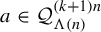 . By Remark 4.1, we have
$a = a_1 \cdots a_ka_{k+1}$
 , for
$a_i \in {\mathcal A}(n)$
 . It follows from Lemma 4.6(3) that

together with the analogous lower bound. Hence, from (5.8) and our inductive hypothesis,

yielding (5.8).
We finally conclude (5.7). As
${\mathcal A}(n)$
 only contains finitely many cylinders, the value

is finite. Let
$b \in {\mathcal Q}^{ s } \cap {\mathcal A}(n)$
 with
$s \in \{1,\ldots , n\}$
 . It follows from Lemma 4.6(1) that

Choose  so that
$2 M / N_0 < \varepsilon / 4$
 . For every
$\ell> N_0$
 and
$a \in {\mathcal Q}^\ell _{\Lambda (n)}$
 , relation (5.9) together with (5.8) implies that
$( {\overline {\tau }}_{ \ell } / \tau _{ \ell } )(a) \in B_{ \varepsilon } ( {\overline {p}} )$
 . This proves the lemma.
5.3 Geometric properties of
${\mathcal A}(n)$

For each n large enough so that Proposition 5.2 holds, let
${\mathcal A}(n)$
 be as provided by Proposition 5.2 and let
$\Lambda (n) = \Lambda ( {\mathcal A}(n) )$
 .
Lemma 5.6. There exists a
$C'> 0$
 such that
$\dim _{\mathrm {H}} \Lambda (n)> 1 - C'/n$
 for all n sufficiently large.
Proof. Consider the function
$h \colon [0,1] \to {\mathbb R}$
 given by

Let  so that, by (4.2),
$h ( s(n) ) = 1$
 . It follows from item (2) in Proposition 5.2 that

and this property holds for all n sufficiently large. We get

giving that
$h'(t) \ge Cn \log \unicode{x3bb} $
 . It follows that

Using Lemma 4.3, with the above, we get

Letting  , the assertion follows.
Fix  to be the geometric measure for
$F^n|_{\Lambda (n)}$
 whose existence is guaranteed by Lemma 4.4.
Lemma 5.7. For all n sufficiently large, there exists an
$N_1 = N_1 ({\mathcal A}(n))$
 so that

Proof. As m is geometric for
$F^n|_{\Lambda (n)}$
 , by (4.6), there exists an
$E(n)> 0$
 so that

Using (4.4), we can choose
$N_1 = N_1 ({\mathcal A}(n)) \in {\mathbb N}$
 so that for
$\ell \ge N_1$
 ,

If
$n> 2C^\prime / \varepsilon $
 , then Lemma 5.6 ensures
$\dim _{\text {H }} \Lambda (n) \ge 1 - \varepsilon /2$
 . Combining this with (5.11) and (5.12) concludes the proof.
5.4 Proof of Proposition 5.1
Fix n large enough so that Lemma 5.7 and Proposition 5.2 hold. Let
${\mathcal A} = {\mathcal A}(n) \subset {\mathcal Q}^n$
 be as in Proposition 5.2 and let
$N_0,N_1$
 be as in Lemmas 5.5 and 5.7. Fix
 and let m be the geometric measure for
$F^n|_{\Lambda ( {\mathcal A})}$
 whose existence is guaranteed by Lemma 4.4. Then, Lemmas 5.5 and 5.7 yield assertion (5.2). Moreover,
$m ( \Lambda ( {\mathcal A} ) )= 1$
 and
$F^n ( {\mathcal A} ) = {\mathcal Y}$
 by item (3) of Proposition 5.2.
Fix
$i \in \{ 1 , \ldots , L\}$
 . As
$Y_i \cap {\mathcal A}$
 is a finite collection of intervals, we know from (4.6) that

where
$r = \min _{ a \in {\mathcal A} \cap Y_i } |a|$
 for some
$E'> 0$
 . The latter is strictly positive by item (2) of Proposition 5.2. This concludes the proof.
6 Proof of Corollary 2.9
Throughout this section, we fix an arbitrary
${\overline {p}} \in {\mathcal S}$
 . We are going to show that

To do so, we first construct a fractal set
$\Gamma $
 , see §6.1. In §6.2, we construct a Borel probability measure supported on
$\Gamma $
 . Section 6.3 states some auxiliary results. In §6.4, we show
$\Gamma \subset \mathscr {G} (\nu _{\overline {p}})$
 . In §6.5, we prove
$\dim _{\mathrm {H}} ( \Gamma ) = 1$
 , which implies (6.1).
6.1 Construction of a fractal set
$\Gamma $

Fix a sequence
$(\varepsilon _{ i })_{i\ge 0} \subset (0,1)$
 such that
$\lim _{i\to \infty }\varepsilon _{ i } = 0$
 . For each
$i \ge 0$
 , fix

as given by Proposition 5.1.
Let
$(k_{ i })_{i \ge 0} \subset {\mathbb N}$
 be an arbitrary sequence of integers. In the remainder of this subsection, we construct a fractal set
$\Gamma = \Gamma ( (k_i)_i )$
 which will depend on this sequence. The precise choice of
$(k_i)_{i}$
 , and hence the precise choice of
$\Gamma $
 , will be fixed in §6.3. Set

and define

Heuristically, the set
$\Gamma $
 consists of points that enter a neighborhood of
$\Lambda _i$
 at time
$t_i$
 and spend time
$k_in_i$
 close to
$\Lambda _i$
 before moving close to
$\Lambda _{i+1}$
 at time
$t_{i+1}$
 . Note that for each
$i\ge 0$
 ,
${\mathcal B}_{ i } \subset {\mathcal Q}^{ t_{ i } }$
 and that the collection
${\mathcal B}_{ i }$
 covers
$\Gamma $
 . By definition, the collections
$({\mathcal B}_i)_i$
 are ‘nested’ in the sense that every element in
${\mathcal B}_{i+1}$
 is a subset of an element of
${\mathcal B}_i$
 for every i.
Lemma 6.1.
$\Gamma $
 is non-empty and compact.
Proof. It is enough to check that for every index
$i\ge 0$
 for every
$a\in {\mathcal A}_{i+1}$
 , there exists
$a'\in {\mathcal A}_i$
 such that
$F^{n_i}(a')\supset a$
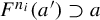 . This follows from the fact that Proposition 5.1 ensures
$F^{n_i} ( {\mathcal A}_i ) = {\mathcal Y}$
 . So, every
${\mathcal B}_i$
 is non-empty and the intersection in (6.3) is the intersection of a nested sequence of compact sets. This implies the assertion.
6.2 Construction of m
We now construct a Borel measure m on Y satisfying
$m ( \Gamma ) =1$
 . We first define m on cylinders
$b a \in {\mathcal Q}^{t_i + s}$
 , where
$b\in {\mathcal Q}^{t_i}$
 and
$a \in {\mathcal Q}^{s}$
 for
$s = 1,\ldots ,k_{i}n_{i}$
 , inductively on i. For
$i = 0$
 ,
$s =1,\ldots ,k_1n_1 $
 , and
$a \in {\mathcal Q}^s$
 , we set

Proceeding inductively, for
$i \ge 1$
 ,
$s=1,\ldots ,k_{i}n_{i}$
 , and
$b a \in {\mathcal Q}^{t_i + s}$
 with
$b \in {\mathcal Q}^{t_i}$
 and
$a\in {\mathcal Q}^s$
 , we define

where

Remark 6.2. As
$F^{t_i} (b) \in {\mathcal Y}$
 , Proposition 5.1 ensures that
$C_i (b)> 0$
 for all
$b \in {\mathcal B}_i$
 .
This defines m on all of
${\mathcal Q}^*$
 . One readily checks that this extends to a Borel probability measure on Y. By construction,
$m({\mathcal B}_i) = 1$
 for every
$i\ge 1$
 , and, in particular,
$m(\Gamma )=1$
 .
6.3 Choice of the sequence
$(k_i)_i$

In the section, we fix the choice of the sequence
$(k_i)_i$
 . First, we introduce

and

For every
$x\in \Gamma $
 and each
$i\ge 0$
 , and
$s = 1,\ldots , k_{i}n_{i}$
 , define the cylinders

such that

In what follows, we will regularly suppress the dependence of the associated
$b_i$
 and
$a_i$
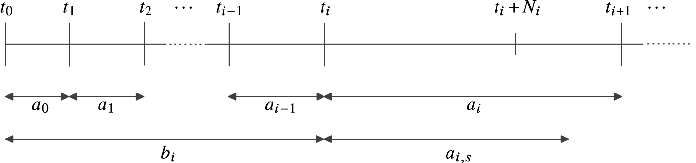
 on x to ease notation. See Figure 3.


We can now state our precise conditions on
$(k_i)_i$
 .


Remark 6.3. Condition (6.10) enables the application of Proposition 5.1, compare (6.2).
By our recursive decomposition into symbolic blocs
$b_{i+1}=b_ia_i$
 , the asymptotic growth of
${\overline {\tau }}/\tau $
 is essentially determined by the ‘immediate past’
$a_i$
 : see the proof of Lemma 6.8 where conditions (6.11) and (6.12) enable estimates (6.20) and (6.22), respectively. Analogous arguments are used to prove Lemma 7.1.
Conditions (6.13)–(6.14) and (6.15)–(6.16) control that arising distortion terms are small (see the proof of Lemma 6.6 and estimates (6.24) and (6.25), respectively).
In the remainder of the section, we prove the following proposition.

We divide the proof into the following lemmas.

Proof. Note that the collection
$\{ b_i (x) \colon x \in \Gamma \}$
 is finite. We also know that the quantities on the tops of the fractions in (6.13) and (6.14) depend on
$k_0,\ldots ,k_{i-1}$
 , but not
$k_i$
 . So, there exists some constant
$L_i < +\infty $
 which is independent of
$k_i$
 (but may depend on
$k_0,\ldots ,k_{i-1}$
 ) such that

We know from Remark 4.2 that
$|\!\log |a_i(x)|| \ge k_{i} n_i \log \unicode{x3bb} $
 . We also know from (6.17) that
$|\!\log m_{i} (a_i)| / \log |a_{i} | \in B_{\varepsilon _i} (1)$
 . In particular, we must have that

So, we can choose
$k_i$
 recursively to grow fast enough so that (6.13) and (6.14) hold.
For what follows, recall from Proposition 5.1 that

Lemma 6.6. If (6.13) and (6.14) hold, then for every
$x \in \Gamma $
 ,

Proof. Let
$x\in \Gamma $
 and consider the associated sequence
$(a_i)_i$
 and
$(b_i)_i$
 in (6.8) and (6.9). Using the definition of m in (6.4), the bounded distortion of F in (4.4), we get

Using (6.17), together with (6.13) and (6.14), we find the lower bound

Analogously, we obtain the upper bound

Taking the limit as
$i\to \infty $
 concludes the proof.

Proof. Suppose that
$(k_i)_i$
 is chosen to grow fast enough so that (6.13) and (6.14) hold by Lemma 6.5. The top of the fractions in (6.15) and (6.16) do not depend on the choice of sequence
$(k_i)_i$
 . However, we know that

Moreover, Lemma 6.6 tells us that then,

Choosing
$(k_i)_{i}$
 to grow sufficiently quickly ensures that (6.15) and (6.16) hold.
Proof of Proposition 6.4
Conditions (6.10) and (6.12) are satisfied whenever
$k_i$
 is chosen to be large enough. Moreover, the top of the fraction in (6.11) depends only on
$k_0,\ldots ,k_{i-1}$
 and not on
$k_i$
 . These observations together with Lemmas 6.5 and 6.7 ensure that
$(k_i)_i$
 can be chosen such that (6.10)–(6.16) hold. This completes the proof.
For the remainder of this section, we fix
$(k_i)_i$
 satisfying (6.10)–(6.16) and fix the corresponding choices of
${\mathcal B}_i$
 ,
$\Gamma $
 , and m.
6.4 Limit behavior of points in
$\Gamma $

Lemma 6.8. For all
$x\in \Gamma $
 ,
${\mathcal V}(x) = \nu _{ {\overline {p}}}$
 .
Proof. Let
$x \in \Gamma $
 . By Corollary 3.2, it is enough to show that
${\mathcal T}(x) = {\overline {p}}$
 .
Recall the definition of the associated cylinders
$a_{i,s} \in {\mathcal Q}_{\Lambda _i}^{s}$
 ,
$a_{i} \in {\mathcal Q}_{\Lambda _i}^{k_in_i}$
 , and
$b_i \in {\mathcal B}_i$
 in (6.8) and (6.9). Recall from Proposition 5.1 that

We also make use of the following inequalities which come from the definition (6.6) and the fact that
$\tau \ge 1$
 :

for all
$s = 1,\ldots , k_in_i $
 .
Recalling that
$b_i = a_0 \cdots a_{i - 1}$
 , we can write
$b_{ i + 1 } = b_i a_i$
 . Then, from Lemma 4.6(2) together with (6.19) and (6.11),

So, using (6.18) with
$s = k_{ i }n_{i}$
 , we obtain

We now fix
$i \ge 1$
 and consider the intermediate times
$t_{i} + s$
 where
$s= 1 ,\ldots , k_in_{ i } - 1$
 . Let us first consider the range
$s = 1 , \ldots , N_{i} - 1$
 . By Lemma 4.6(1) together with (6.19) and (6.12), we have that

So, using (6.21), we know that

Now, let us consider the range
$s = N_{ i }, \ldots , k_{i}n_{i} - 1$
 . By Lemma 4.6(3), we know that

Thus, by (5.7) and (6.21), we find that

As we assume that
$\varepsilon _i\to 0$
 , this proves
${\mathcal T}(x) = {\overline {p}}$
 .
6.5 Hausdorff dimension of
$\Gamma $

Let us recall the definition of Hausdorff dimension (see [Reference FalconerFal97] for further details). Given
$S\subset [0,1]$
 and
$d\ge 0$
 , let

where the infimum is taken over all countable covers
$\{U_k\}$
 of S. The Hausdorff dimension of S is defined by
 .
Lemma 6.9.
$\dim _{\mathrm {H}} \Gamma = 1. $

Proof. Let
$x\in \Gamma $
 . Recall the definition of the associated cylinders
$a_{i,s} \in {\mathcal Q}_{\Lambda _i}^{s}$
 ,
$a_{i}\in {\mathcal Q}_{\Lambda _i}^{k_in_i}$
 , and
$b_i\in {\mathcal B}_i$
 in (6.8) and (6.9). We will show that

Set

and recall from Lemma 6.6 that
$\lim _{i\to \infty } \ell _i = 1$
 . Consider first the range
$s = 0, \ldots , N_i$
 . We proceed as in the proof of Lemma 6.6. Using the definition (6.4), the bounded distortion (see Remark 4.2)

where in the final inequality, we have used (6.15) and (6.16).
Now, let us consider the range
$s = N_i, \ldots ,k_in_{i}$
 . We begin as before, but this time, we make use of (4.7) to obtain

Then, we notice, using (6.15) and (6.16), that

Recalling (6.17), we have
$\log m_i (a_{i,s}) / \log |a_{i,s}| \ge 1 - \varepsilon _i$
 . Combining this with (6.24), (6.25), and (6.26), we obtain

Proceeding in the same way as above, one can find analogous upper bounds for (6.24), (6.25), and (6.26), which yield

As
$\lim _{i \to \infty } \underline {\delta }_i = \lim _{ i \to \infty } \overline {\delta }_i = 1$
 , we obtain (6.23).
Denote by
${\mathcal Q}^\ell (x)$
 the element of the partition
${\mathcal Q}^\ell $
 which contains x. Recall that, by the above, for every
$x\in \Gamma $
 , for
$\ell =t_i=k_0n_0+k_1n_1+\cdots +k_{i-1}n_{i-1}$
 associated with x, there is a sequence
$b_i(x)=a_0(x)a_1(x)\cdots a_{i-1}(x)$
 , where
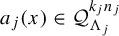
$a_j(x)\in {\mathcal Q}^{k_jn_j}_{\Lambda _j}$
 and

Likewise, for
$\ell =t_i+s$
 , with
$s=1,\ldots ,k_in_i$
 ,

From the above, we get

As the refinements of the partition
${\mathcal Q}$
 separate points, the assertion of the lemma then follows from the mass distribution principle (compare [Reference FalconerFal97, Ch. 2]).
7 Proof of Theorem A
In this section, we prove Theorem A. We will follow the same structure as for the proof of the special case in §6. The only significant difference is how the sets
${\mathcal A}_{i}$
 are chosen in the construction of the fractal set
$\Gamma $
 . Throughout this section, we fix a closed connected subset
${\mathcal C} \subset {\mathcal S}$
 . In §7.1, we construct a set
$\Gamma $
 . In §7.2, we show that
$\Gamma \subset \{ x \colon {\mathcal V}(x) = \pi {\mathcal C} \}$
 . In §7.3, we conclude
$\dim _{\mathrm {H}} \Gamma = 1$
 , which proves Theorem A.
7.1 Construction of a fractal set
$\Gamma $

Let
$({\overline {p}}_i)_{i\ge 0} \subset {\mathcal C}$
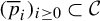 be a sequence whose limit points are equal to
${\mathcal C}$
 and so that
$\lim _{i \to \infty }| {\overline {p}}_{i} - {\overline {p}}_{i + 1 } | = 0$
 . Let
$(\varepsilon _i)_{i\ge 0} \subset (0,1)$
 be such that
$\lim \varepsilon _i = 0$
 . For each
$i\ge 0$
 , let
 ,
${\mathcal A}_i = {\mathcal A}( \varepsilon _i ,{\overline {p}}_i) \subset {\mathcal Q}^{n_i}$
 ,
$\Lambda _i = \Lambda ( {\mathcal A}_i )$
 ,
$N_i = N( \varepsilon _i,{\overline {p}}_i)$
 , and
$m_i = m ( \varepsilon _i,{\overline {p}}_i)$
 be as given in Proposition 5.1. With these definitions in place, we define
$M_i,E_i$
 as in (6.6). Then, we may repeat verbatim the proof of Proposition 6.4 to give the existence of a sequence
$(k_i)_{i \ge 0}$
 satisfying the conditions (6.10)–(6.16). Fixing such a sequence
$(k_i)_{i}$
 , we set

and define

Repeating the proof of Lemma 6.1, we see that
$\Gamma $
 is non-empty and compact. Following §6.2, we construct a probability measure m on
$\Gamma $
 exactly as before.
7.2 Limit behavior of points in
$\Gamma $

Lemma 7.1.
${\mathcal V}(x) = \pi {\mathcal C}$
 for every
$x\in \Gamma $
 .
Proof. Let
$x \in \Gamma $
 . From Theorem 3.1, it is enough to show that
${\mathcal T}(x) = {\mathcal C}$
 and (3.1) holds.
Recall the definition of the cylinders
$a_{i,s}(x) \in {\mathcal Q}_{\Lambda _i}^{s}$
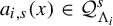 ,
$a_{i}(x) \in {\mathcal Q}_{\Lambda _i}^{k_in_i}(x)$
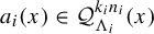 , and
$b_i(x) \in {\mathcal B}_i$
 in (6.8) and (6.9) (see also Figure 3). We suppress the dependence of
$a_{i,s},a_i$
 , and
$b_i$
 on x to ease notation. Recall from item (1) of Proposition 5.1 that

Writing
$b_{i+1} = b_i a_{i}$
 , it follows from Lemma 4.6(2) together with (6.19) and (6.11) that

So, using (7.1) with
$s = k_{ i }n_{i}$
 , we obtain

This gives the conclusion of the lemma along the subsequence
$t_i$
 , in the sense that

We now fix
$i \ge 1$
 and consider the intermediate times
$t_{i} + s$
 , where
$s= 1 ,\ldots , k_{i}n_{i} - 1$
 . Let us first consider the range
$s = 1 , \ldots , N_{i} - 1$
 . By Lemma 4.6(1) together with (6.19) and (6.12), we have that

So, using (6.21), we know that

Now, let us consider the range
$s = N_{ i}, \ldots , k_{i}n_{i}-1, k_{i}n_{i}$
 . By Lemma 4.6(3), we know that

where the inequality holds coordinate-wise. Let
$\delta _i = \max \{ 3\varepsilon _{i-1}, 3\varepsilon _{i} \}$
 , and recall from (7.3) and (7.1) that
$({\overline {\tau }}_{ t_{ i } } / \tau _{ t_{ i } } ) (b_i) \in B_{\delta _i}({\overline {p}}_{i-1})$
 and
$({\overline {\tau }}_{ s } / \tau _{ s } ) (a_{i,s}) \in B_{\delta _i}({\overline {p}}_{i})$
 . Thus,

where
$R_i^{\delta _i}$
 is the
$\delta _i$
 -neighborhood of the d-dimensional rectangle
$R_i$
 that has
${\overline {p}}_i$
 and
${\overline {p}}_{i+1}$
 as vertices and is given by

As
$\lim _{i \to \infty } | {\overline {p}}_i - {\overline {p}}_{i+1} | = 0$
 , and as
$\lim _{i \to \infty } \delta _i = 0$
 , we know that the rectangles
$R^{\delta _i}_{i}$
 accumulate precisely at the limit points
${\mathcal C}$
 of
$({\overline {p}}_i)_i$
 . This concludes that
${\mathcal T}(x) = {\mathcal C}$
 .
To check that (3.1) holds, let
$k\in {\mathbb N}$
 and choose i such that
$t_i\le k< t_{i+1}$
 . Hence, it follows from (7.5) that

As
$k\to \infty $
 , we get
$i\to \infty $
 and hence, the latter tends to
$0$
 . This implies that (3.1) holds and hence proves the lemma.

8 Examples
We consider an interval map
$f \colon X \to X$
 that admits a Markov partition
${\mathcal P}$
 which has
$d\ge 2$
 neutral fixed points
$\{\xi _1,\ldots , \xi _d\}$
 . At these neutral fixed points, we will always assume that we have the following expansion:

We assume that there is a partition
$I_1,I_2,\ldots $
 of X (modulo
$\mathrm {Leb}$
 ) into
$d + d'$
 open sub-intervals, where
$0 \le d' \le + \infty $
 such that each
$I_i$
 is a union of elements in
${\mathcal P}$
 and each restriction
 is a
$C^2$
 diffeomorphism onto its image. (Notice that we do not impose that
$f_i$
 extends to a
$C^2$
 diffeomorphism on the closure of
$I_i$
 .)
Example 8.1. Suppose that
$d' = 0$
 and that each branch of the map is full in the sense that
$f_i(I_i) = (0,1)$
 and monotone increasing. Moreover, we assume that

and that Adler’s distortion condition holds:

In this case, we obtain a map with d full orientation-preserving branches, each of which contains a neutral fixed point satisfying (8.1). In this case, we define

where in the case
$d = 2$
 ,
$\{ \gamma , f \gamma \}$
 is the unique orbit of period 2. The fact that this map satisfies Assumptions 2.1–2.6 for this choice of Y can be found in [Reference Coates, Melbourne and TalebiCMT24, §4.1].
Example 8.2. We can generalize the previous example by allowing an additional
$1 \le d' \le +\infty $
 uniformly expanding branches. As in Example 8.1, we assume that both (8.2) and (8.3) hold, and we set

regardless of the value of d. The fact that such maps satisfy Assumptions 2.1–2.6 can be found in [Reference Coates and MelbourneCM25, Example 5.14].
Example 8.3. Another way which can generalize Example 8.1 is by allowing for critical and/or singular points at the preimages of the neutral fixed points. For simplicity, we will stick to the case that
$d = 2$
 , which was introduced in [Reference Coates, Luzzatto and MuhammadCLM23]. The fact that these maps satisfy Assumptions 2.1–2.6 can be found in [Reference Coates, Melbourne and TalebiCMT24, §4.2].
Acknowledgements
K.G. has been supported (in part) by CAPES—Finance Code 001, CNPq grant 305327/2022-4 and FAPERJ—Carlos Chagas Filho Foundation for Research Support of the State of Rio de Janeiro, Processes E-26/200.371/2023, E-26/200.133/2026. This study was funded by FAPERJ—Carlos Chagas Filho Foundation for Research Support of the State of Rio de Janeiro, Processes SEI E-26/200.371/2023, E-16/2014 INCT/FAPERJ, and E-26/200.027/2025 and 200.028/2025, and by the FAPESP Carlos Chagas Filho Foundation for Research Support of the State of São Paulo Research Foundation grant 2022/16259-2. The authors thank their home institutions for their hospitality while preparing this paper. The authors thank Gabriela Estevez for pointing out the elegant inequality in (4.7) which made many of our arguments less tedious. The authors would also like to also thank Daniel Smania for stimulating conversations at the onset of this project and for showing us [Reference Moreira and SmaniaMS14], which inspired some of the ideas in §5. A big thank you also to Fabio Tal for giving the key idea which led to the removal of the assumption that
${\mathcal C}$
 is convex in Theorem A.