2.1. Results for the directed k-neighbor graph

As a first step, we study the cases where the occurrence of percolation is deterministic. On the one hand, choosing only one neighbor is never enough for percolation; on the other hand, choosing a sufficiently large number of neighbors leads to the almost-sure existence of a path connecting the origin to infinity.

Let us sketch why these statements are true.

1. (i) If there exists a path starting from the origin and reaching an $\ell_1$ -distance n from the origin, then this path is unique and has at least n steps. But such a path exists with probability at most $2d \cdot (2d-1)^{n-1} \cdot (2d)^{-n}$ , which converges to zero as n tends to infinity. Here, $2d \cdot (2d-1)^{n-1}$ is an upper bound for the number of n-step paths in $\mathbb{Z}^d$ .

2. (ii) The reason this holds is that the maximal distance to the origin is strictly increasing between generations. To be more precise, for $n \in \mathbb{N}_0$ we define $G_n$ , the nth generation of vertices, inductively as follows. We initialize $G_0=\{0\}$ , and define $G_{n+1}$ as the set of those neighbors chosen by the vertices of $G_n$ (according to the definition of the k-DnG) that are not included in $\cup_{j=0}^nG_j$ . Since $k \geq d+1 = d$ , among any k neighbors of any vertex x there exists one, say y, whose $\ell_1$ -norm $\|y\|_1$ is larger than $\|x\|_1$ . In this way, we can show via induction that, for all $n \in \mathbb{N}$ , $\max_{x \in G_n}\|x\|_1 < \max_{x \in G_{n+1}}\|x\|_1$ . This then implies that there exists an infinitely long directed path starting at the origin.

Let us now turn our attention towards the intermediate supercritical percolation phase. Here, our tools for the proof are restricted to sufficiently high dimensions d.

The proof can be found in Section 4.1 and mainly relies on a variation of the technique established in [Reference Cox and Durrett5] plus precise estimates on the probability that two independent simple oriented random walks meet each other and then take a common step. In fact the proof of Theorem 2.1 establishes positive probabilities for the existence of infinite, self-avoiding, and monotone paths, i.e. paths with strictly increasing $\ell_1$ -norm.

Last, but not least, we come to the question of monotonicity with respect to the parameters. It is also easy to see that for $d \geq k$ we have $\theta^{\rm D}(k,d) <1$ and, by the assertion of Remark 2.1, $\theta^{\rm D}(k,d)=1$ for $d\le k-1$ , so $d\mapsto \theta^{\rm D}(k,d)$ can be decreasing. However, in view of similar results in the continuum [Reference Häggström and Meester7], it seems reasonable to assume that $d\mapsto \theta^{\rm D}(k,d)$ is increasing for large d. At least, we can deduce the following monotonicity along diagonals of the parameter space.

The proof of Theorem 2.2 can be found in Section 4.1 and is based on a coupling argument. We will see that it is essential that both k and d increase by one to make the coupling work. For example, issues arise when trying to deduce a similar coupling between the settings $k=d=2$ and $k=2,d=3$ . Though we expect percolation occurs in both settings, a similar coupling would give rise to a two-dimensional model where some vertices have only out-degree one. In such a case, it seems that the additional edges that appear in the 2-DnG in two dimensions are pivotal in the sense that they enable percolation to occur, whereas it may not occur without the presence of these edges. Still, we expect that if we restrict ourselves to parameters $k \leq d$ a similar relation between the d-dimensional and $(d+1)$ -dimensional settings should exist. We state this in Conjecture 3.2 below.

2.2. Results for the undirected k-neighbor graph

To state our results and proofs for the k-UnG we first introduce the following notation. It is clear that $\theta^{\rm U}(k,d) \geq \theta^{\rm D}(k,d)$ for any $k,d\in \mathbb{N}$ because any directed edge in the k-DnG corresponds to an undirected edge in the k-UnG (and at most two directed edges can correspond to the same undirected edge). This way, Theorem 2.1 Remark 2.1(ii) also hold with $\theta^{\rm D}$ replaced by $\theta^{\rm U}$ everywhere. Moreover, we can now also deal with lower dimensions.

However, even in the undirected sense, $k=1$ is still not sufficient for percolation in any dimension $d \in \mathbb{N}$ .

We recently learned that Proposition 2.1 directly follows from results in [Reference Hirsch, Holmes and Kleptsyn9] studying a more general percolation model. Nevertheless, since the notation in [Reference Hirsch, Holmes and Kleptsyn9] is quite different, we also present our proof for the reader’s convenience and for completeness.

2.3. Results for the bidirectional k-neighbor graph

Clearly, $\theta^{\rm B}(k,d) \leq \theta^{\rm D}(k,d)$ , so we already know that, if each vertex chooses a single neighbor, the bidirectional model will not percolate. A stronger result holds for this model, however. The following lemma presents an upper bound for k in terms of d for which we can verify that the bidirectional model does not percolate. To state this lemma, let us denote by c(d) the connective constant of $\mathbb{Z}^d$ (see, e.g., [Reference Grimmett6]), which is defined by $c(d) \,:\!=\, \lim_{n \to \infty}c_n(d)^{1/n}$ , where $c_n(d)$ is the number of self-avoiding paths of length n in the d-dimensional hypercubic lattice that start at the origin. Via a quick subadditivity argument we can show that the limit c(d) actually exists and satisfies $d < c(d) < 2d -1$ .

Let us note that this result can be interpreted in two ways. First, for given d, it guarantees absence of percolation for all sufficiently small k and, for example, $\theta^{\rm B}(2,d)=0$ for any $d\geq 2$ (while it is clear that $\theta^{\rm B}(2,1)=1$ ), $\theta^{\rm B}(3,d)=0$ for any $d \geq 3$ , and $\theta^{\rm B}(4,d)=0$ for any $d \geq 6$ , as can be seen from the lower bounds on c(d) in [Reference Hara, Slade and Sokal8, Table 1] (e.g. $c(6)\geq 10.874\,038$ ). However, also for fixed k, since $2d(2d-1)/c(d)>2d$ , for sufficiently large d, there is no percolation thanks to Lemma 2.1. This is because, in high dimensions, it is unlikely for two neighboring vertices to pick the same connecting edge. This behavior is rather different from the case of the k-DnG and the k-UnG, where there is percolation for all $k \geq 3$ in all sufficiently high dimensions.

Table 1.

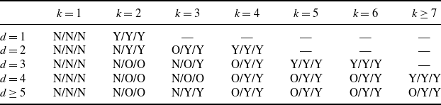
Percolation results and open cases for the BnG/DnG/UnG. For given k and d, ‘Y’ means that the given graph percolates, ‘N’ means that it does not, while ‘O’ means that the given case is (at least partially) open. Percolation in the case $k=d=2$ was verified in [Reference Coupier, Henry, Jahnel and Köppl4]; see Section 3.1 for a discussion on the case $k=2$ for general d.

The proof strategy for Theorem 2.3 is to verify that percolation occurs when restricting ourselves to a two-dimensional plane, see Section 4.2. This approach is also applicable in the bidirectional model, and yields the following result.

An application of the upper bound $c(2)\leq 2.679\,192\,495$ from [Reference Pönitz and Tittmann17] for the connective constant of $\mathbb{Z}^2$ immediately yields the following corollary.

This corollary allows us to verify percolation, e.g., for the $(2d-1)$ -BnG for $d \geq 3$ , for the $(2d-2)$ -BnG for $d \geq 5$ , for the $(2d-3)$ -BnG for $d \geq 8$ , and for the $(2d-4)$ -BnG for $d \geq 10$ . (Thus, the smallest-dimensional positive percolation result that we obtain from the corollary is that $\theta^{\rm B}(5,3) >0$ .)

Note that, compared to the dimension d, we always need rather large k to percolate. In high dimensions, we can improve the ratio slightly by using that the k-BnG model (just as the k-UnG model) in any dimension d is a 1-dependent Bernoulli bond percolation model. Let

\[ p_{\sup}(\mathbb{Z}^d)=\sup\{p\in(0,1)\colon\text{some 1-dependent bond percolation model does not percolate}\}.\]

According to a recent result in [Reference Balister, Johnston, Savery and Scott3], we have $\lim_{d\to\infty} p_{\sup}(\mathbb{Z}^d) \leq 0.5847$ . This, together with the fact that the k-BnG model (just as the k-UnG model) in any dimension d is a 1-dependent bond percolation model where each edge is open with probability $p=k^2/(4d^2)$ , immediately implies the following proposition.

Let us remark that another result in [Reference Balister, Johnston, Savery and Scott3] is that $p_{\sup}(\mathbb{Z}^2) \leq 0.8457$ . This, together with the assertion that $p_{\sup}(\mathbb{Z}^d) \leq p_{\sup}(\mathbb{Z}^{d-1})$ , yields that for $\alpha>2\sqrt{0.8457}$ we have $\theta^{\rm B}(\lfloor \alpha d \rfloor, d)>0$ . However, this statement is weaker than Proposition 2.2 given that $2\sqrt{0.8457} \approx 1.8392 > \sqrt{4(1-1/2.679\,192\,495)}$ .

Of course, the k-UnG model is also a 1-dependent bond-percolation model, but the same approach unfortunately does not yield any new results in this case. Indeed, here, each edge is open with probability $p=k(4d-k)/(4d^2)$ . Thus, for $k=d$ it always holds that $p=3/4<0.8457$ , while for $k>d$ (and for $d \geq 2$ even for $k \geq 4$ ) we already know that $\theta^{\rm D}(k,d)=1$ .

We summarize our results in Table 1.

3.1. Directed k-neighbor graphs

Until very recently, for the k-DnG the most pressing open question was whether it percolates for $k=2$ in $d=2$ . Very recently, the first two authors of this paper together with David Coupier and Benoît Henry published a preprint proving that it indeed percolates for $k=d=2$ [Reference Coupier, Henry, Jahnel and Köppl4, Theorem 2.3]. According to simulations (see Figure 1), the proportion of vertices that can be reached from the origin is actually quite high. The heuristic that it is easier for the DnG to percolate in higher dimensions suggests the following conjecture.

Figure 1.

Samples of the 2-DnG in boxes with side length n. The colored vertices are those contained in the connected component of the origin.

Note that the complement of the k-DnG in d dimensions with respect to $\mathbb{Z}^d$ , i.e. the graph with vertex set $\mathbb{Z}^d$ and the edge set formed by all nearest-neighbor edges of $\mathbb{Z}^d$ not contained in the k-DnG, is in distribution a $(2d-k)$ -DnG. So the 2-DnG is an example of phase coexistence in a self-complementary (directed) graph in two dimensions.

With regards to the monotonicity statement, Theorem 2.2, we expect a corresponding statement also to hold along the diagonal of the (k, d)-plane grid.

Given percolation in the 2-DnG for $d=2$ , one possible way to prove Conjecture 3.1 would be to verify Conjecture 3.2, but at least for higher dimensions d there might be simpler arguments making use of intersection properties of random walks to show that $\theta^{\rm D}(2,d) > 0$ . Of course, this would also imply that $\theta^{\rm U}(k,d)>0$ for all $k,d\geq2$ .

3.2. Bidirectional k-neighbor graphs

For the bidirectional model the most intriguing question seems to be what the smallest $k=k(d)$ is such that $\theta^{\rm B}(k(d),d)>0$ holds for all d (or at least for all d sufficiently large). Heuristically, we would expect that we do not percolate when the expected degree of a vertex is less than two, because the chance of backtracking, i.e. not getting a new edge, is then too large. However, as soon as we have an expected degree of at least two, we could imagine that this is sufficient to percolate, since we usually get at least one new edge in each step while walking along a path. At least in low dimensions (which are still accessible for numerical computations) the numerical tests seem to support the following conjecture – see Figures 2 and 3.

Figure 2.

Samples of the 3-BnG in boxes with side length n. The colored vertices are those contained in the connected component of the origin.

Figure 3.

Probability of reaching the boundary of boxes $S_n$ of varying side length n in the d-BnG for $d \in \{2,3,4,5\}$ (sample size: 10 000).

In particular this would imply that the d-BnG does not percolate for dimensions $d=2,3$ but percolates for $d \geq 4$ , and that the 3-BnG percolates in $d=2$ .

3.3. XOR percolation

Let us briefly consider another variant of lattice k-neighbor graphs, namely the exclusively unidirectional k-nG (k-XnG), in which we open an undirected edge between two vertices whenever exactly one of them chooses the other one as one of its k chosen neighbors. The letter X refers to the ‘XOR’ (exclusive ‘or’) in the edge-drawing rule.

Although the parameter k of the k-XnG can range between 1 and 2d (just as for the k-BnG, k-DnG, and k-UnG), actually it suffices to consider $1 \leq k \leq d$ , thanks to the following considerations.

Of course, the assertion of Remark 3.1 also holds for $k=2d$ if we define the 0-XnG as $\mathbb{Z}^d$ with no edges, from which it is clear that $\theta^{\rm X}(2d,d)=0$ for all d, where we write $\theta^{\rm X}$ for the percolation probability of the XnG analogously to (2.1). Hence, we can limit our analysis to the cases $1\le k\le d$ .

It is also easy to see that, since the k-XnG is a subgraph of the k-UnG, we have $\theta^{\rm X}(1,d)=0$ for all $d \geq 1$ and thus, by Remark 3.1, $\theta^{\rm X}(2d-1,d)=0$ for all d. Moreover, the 2-XnG is also not percolating in one dimension, so the first non-trivial case is $k=d=2$ ; see Figure 4 for some simulations.

Figure 4.

Samples of the 2-XnG in boxes with side length n. The colored vertices are those contained in the connected component of the origin.

Since the probability of an edge being open in the k-XnG is given by $k(2d-k)/(2d^2)$ , which is maximized at $k=d$ with maximum value $\frac{1}{2}$ , the d-XnG seems to be critical in dimension d. Moreover, for $k\ge 2$ , and $e_1, e_2$ edges that share a common vertex,

\begin{equation*} \mathbb{P}(e_1,e_2\text{ open})=\frac{(2d-k)(k(4k-1)(2d-k)-k^2)}{8d^3(2d-1)} \leq \frac{k^2(2d-k)^2}{4d^4}=\mathbb{P}(e_1\text{ open})^2,\end{equation*}

with equality if and only if $k=d$ . Thus, the model features negative correlations that decrease in $k\in\{2,\dots,d\}$ and in particular, for $k=d$ , we even have pairwise independence. This, together with the fact that, for fixed d, the probability of an edge being open in the k-XnG increases, allows us to formulate the following conjecture.

Despite our heuristic justification, it is not clear to us how to verify this conjecture. In particular, we are not aware of a coupling between the k-XnG and the l-XnG for $1 \leq k < l \leq d$ , while the k-DnG (respectively k-UnG, k-BnG) is a subgraph of the l-DnG (resp. l-UnG, l-BnG) whenever $1 \leq k \leq l \leq 2d$ .

Let us finally mention that, in view of the first-moment method for the proof of existence of subcritical regimes (see, for example, Lemma 2.1) we would need to establish $\mathbb{P}(e_1\text{ open}\mid e_2\text{ open})c(d)<1$ , which is unfortunately not true for any $2\le k\le d$ . Also, none of the methods we have used to prove existence of supercritical percolation regimes seem to apply to the k-XnG, so determining whether it actually percolates for certain choices of d and k remains a goal for our future research.

Focusing on the case $k=2$ , we have performed simulations that suggest absence of percolation for $d=2$ – see Figures 5(a) and 5(b).

Figure 5.

Numerical experiments for the XnG in dimensions $d=2,3$ (sample size=1000).

Based on this and Figure 5(c), we can at least formulate the following conjecture.

3.4. In-percolation and strong percolation

As already mentioned in the introduction, our notion of directed percolation (2.1) corresponds to out-percolation in [Reference Balister and Bollobás2]. In this paper, we have not developed any specific proof techniques for strong percolation or in-percolation. Nevertheless, it is clear that, for fixed d and k, percolation in the k-BnG implies strong percolation, while strong percolation implies both in- and out-percolation in the k-DnG. Moreover, in- or out-percolation in the k-DnG implies percolation in the k-UnG, analogously to the continuum case (where these implications were mentioned in [Reference Balister and Bollobás2]). Hence, our positive percolation results for the k-BnG yield similar results for strong percolation, and our negative (out-)percolation results for the k-DnG imply the absence of strong percolation. Furthermore, writing

\[ \theta^{{\rm D}'}(k,d) = \mathbb{P}(\text{there exists an infinite directed path in the}\ \textit{k}\text{-DnG ending at }o) \]

for the analogue of $\theta^{\rm D}(k,d)$ for in-percolation, we have $\theta^{{\rm D}'}(1,d)=0$ , since $\theta^{\rm U}(1,d)=0$ holds thanks to Proposition 2.1.

One reason why we could be led to believe that Conjecture 3.6 is true is the following simple argument, which is based on the mass-transport principle (see, e.g., [Reference Lyons and Peres16, Chapter 8]). Consider the function $F(x,y;\omega) \,:\!=\, \mathbf{1}_{\{x \to y\}}(\omega)$ , $x,y\in \mathbb{Z}^d$ , where $\omega$ is a realization of the directed k-DnG on $\mathbb{Z}^d$ . This function F is clearly diagonally invariant with respect to lattice shifts, i.e. $F(x+z,y+z;\,\omega+z) = F(x,y;\,\omega)$ . So, if we let $\overrightarrow{C_0}$ denote the out-component of the origin and $\overleftarrow{C_0}$ denote the in-component, then the classical mass-transport principle [Reference Lyons and Peres16, p. 274] implies that

\begin{equation*} \mathbb{E}\big[\lvert\overrightarrow{C_0}\rvert\big] = \sum_{x \in \mathbb{Z}^d}\mathbb{E}[F(0,x;\cdot)] = \sum_{x \in \mathbb{Z}^d}\mathbb{E}[F(x,0;\cdot)] = \mathbb{E}\big[\lvert\overleftarrow{C_0}\rvert\big].\end{equation*}

Hence, if we have out-percolation at parameters d, k, then at least the expected size of the in-cluster is also infinite, and vice versa. A sharp-threshold result (including exponential tails of the cluster size distribution in the subcritical phase) would yield the conjecture.

Let us further remark that Conjecture 3.6 is not known either in the continuum case. Without such a result, it seems that in-percolation is in general more difficult to deal with than out-percolation, due to increased combinatorial complexity. For example, showing that the 1-DnG does not percolate was relatively straightforward (cf. the proof of Remark 2.1(i)), but proving the lack of in-percolation in the same graph (cf. the proof of Proposition 2.1) already presented more challenges. Further, in the two-dimensional Poisson case in the proof of [Reference Balister and Bollobás2, Theorem 2], the authors showed directly that out-percolation occurs for $k=13$ , but for in-percolation for the same k the same method did not work. They derived that their arguments for out-percolation actually imply strong percolation and therefore also in-percolation.

We have seen that, for d large, out-percolation in the k-DnG already occurs for $k=3$ , while for the k-BnG percolation definitely requires $k=\Omega(\sqrt d)$ , and all the examples where we have verified percolation are such that $k>d$ . It is an interesting open question whether strong percolation is closer to directed (out-)percolation than to bidirectional percolation in this respect. The aforementioned arguments of [Reference Balister and Bollobás2] suggest the former.

4.1. Proofs for the k-DnG

In this section, we carry out the proofs of Theorems 2.1 and 2.2.

Proof of Theorem 2.1. We follow [Reference Cox and Durrett5, Section 2]. Since we have already verified the assertion of Remark 2.1, without loss of generality we will assume that $k \leq d$ . Let $\mathcal R_n$ denote the set of oriented paths from the origin to level n (i.e. all vertices at $\ell_1$ -distance n) with strictly increasing $\ell_1$ -distance that stay within the first closed quadrant, in other words all vertices on the path have non-negative coordinates, and let $N_n$ be the number of open paths in $\mathcal R_n$ . Then $W_n=(2/k)^nN_n$ is a martingale with respect to $\mathcal F_n$ , the sigma-algebra generated by the first n steps of a simple and symmetric oriented random walk T with $T_0=o$ and $T_{n+1}=T_n+e_i$ , where i is uniformly chosen from $\{1,\dots ,d\}$ for all $n\in\mathbb{N}_0$ . Indeed, using the fact that the expected number of monotone (i.e. with respect to $\ell_1$ -distance increasing) edges is given by the expectation of a hypergeometric random variable, i.e.,

\begin{equation*} \sum_{\ell=0}^k \ell\binom{d}{\ell}\binom{d}{k-\ell}\big/\binom{2d}{k}=\frac{k}{2}, \end{equation*}

and we can use independence to see that $\mathbb{E}[N_{n+1}\mid\mathcal F_n]=kN_n/2$ .

Since $\mathbb{E}[W_1]=1$ , we can apply the martingale convergence theorem to ensure the existence of a random variable W with $W_n\to W$ almost surely. Using the second-moment method, it now suffices to show that $\limsup_{n\uparrow\infty}\mathbb{E}[W_n^2]<\infty$ , since by the Paley–Zygmund inequality we then have that $\mathbb{P}(W>0)>0$ , which implies $\theta^{\rm D}(k,d)>0$ .

For this, note that

\begin{equation*} \mathbb{E}[N_n^2] = \sum_{s,t\in \mathcal R_n}\mathbb{P}(s,t\text{ open}) = \sum_{s,t\in \mathcal R_n}p^{K(s,t)}q^{L(s,t)}p^{2(n-K(s,t)-L(s,t))}, \end{equation*}

where $p=k/(2d)$ denotes the probability that a given edge is open, $q=k(k-1)/(2d(2d-1))$ denotes the probability that two different edges that emerge from the same vertex are open, K(s, t) is the number of joint edges in two paths s and t, and L(s, t) is the number of vertices x in s and t such that s and t do not have a joint edge after x. Now note that $q<p^2$ , which implies that $\mathbb{E}[N_n^2] \leq \sum_{s,t\in \mathcal R_n} p^{2n-K(s,t)}$ . The right-hand side is precisely the same as the right-hand side of the display below [Reference Cox and Durrett5, (2.7)]. Thus, a verbatim application of the arguments of [Reference Cox and Durrett5, Section 2] implies that $\lim_{n\to\infty} \mathbb{E} W_n^2 <\infty$ holds if and only if $p =k/(2d)> \varrho(d)$ , where for two independent (simple, symmetric, nearest-neighbor, oriented) random walks $ S=(S_n)_{n\in\mathbb{N}_0}$ and $ S'=(S'_n)_{n\in\mathbb{N}_0}$ on the first quadrant of $\mathbb{Z}^d$ started from the origin, we define

\[ \varrho(d) = \mathbb{P}(\text{there exists } m\geq 0 \colon S_m = S'_m \text{ and } S_{m+1} = S'_{m+1}). \]

Further, let $\tau_d=\inf\{m \geq 0 \colon S_m= S'_m \text{ and } S_{m+1} = S'_{m+1}\}$ . According to [Reference Cox and Durrett5, p. 155], for all d,

(4.1) \begin{equation} \mathbb{P}(\tau_d=0)=d^{-1}, \qquad \mathbb{P}(\tau_d=1)=0, \qquad \mathbb{P}(\tau_d=2)=d^{-3}-d^{-4}, \end{equation}

and, for $3 \leq \ell \leq d$ , $\mathbb{P}(\tau=\ell) \leq d^{-\ell} \ell!$ , while, for $j\geq 1$ and $\ell \in(jd,(j+1)d]$ ,

(4.2) \begin{equation} \mathbb{P}(\tau=\ell) \leq d^{-1} (2\pi d)^{1/2} \bigg(\frac{{\mathrm{e}}^{-1/13}}{\sqrt{2\pi}}\bigg)^d j^{-({d-1})/{2}}, \end{equation}

so that

(4.3) \begin{align} \varrho(d) & = \mathbb{P}(\tau_d<\infty) \nonumber \\ & \leq d^{-1} + d^{-3} -d^{-4} + \sum_{\ell=3}^d d^{-\ell}\ell! + (2\pi d)^{1/2}\bigg(\frac{{\mathrm{e}}^{-1/13}}{\sqrt{2\pi}}\bigg)^d\sum_{j=1}^{\infty}j^{-({d-1})/{2}} \nonumber \\ & = d^{-1} + d^{-3} -d^{-4} + \sum_{\ell=3}^d d^{-\ell}\ell! + (2\pi d)^{1/2}\bigg(\frac{{\mathrm{e}}^{-1/13}}{\sqrt{2\pi}}\bigg)^d\zeta\bigg(\frac{d-1}{2}\bigg) =\!:\, U(d), \end{align}

where $\zeta$ denotes the Riemann zeta function. To conclude that we do indeed percolate, it suffices to verify that U(d) is less than $k/(2d)$ . In low dimensions we can compute the right-hand side numerically. More precisely, Table 2 shows the smallest values of k such that U(d) is less than $k/(2d)$ , for $d=4,5,6,7$ .

Table 2.

Values of the right-hand side of (4.3) and the smallest k such that this right-hand side is below $k/(2d)$ , for $4 \leq d \leq 7$ .

In particular, we see from Table 2 that $U(d)<k/(2d)$ holds for $k=3$ and $d=7$ . Now, in order to lift this to higher dimensions $d>7$ for the same $k=3$ , we rewrite

\[ 2dU(d) = 2\Bigg(1 + \frac{1}{d^2} - \frac{1}{d^3} + \sum_{\ell=3}^{d}\ell!/d^{\ell-1} + (2\pi)^{1/2}g(d)\zeta\bigg(\frac{d-1}{2}\bigg)\Bigg), \]

with $g(d)=d^{3/2}(\mathrm e^{-1/13}/\sqrt{2\pi})^d$ . Now, observe that, for all $d \geq 4$ , the terms $d^{-2} - d^{-3}$ , $\sum_{\ell=3}^{d} \ell ! / d^{\ell-1}$ , g(d), and $\zeta((d-1)/2)$ are all decreasing in d. Therefore, for a given k, if $2 d U(d) \leq k$ , then $2d' U(d') \leq k$ for all $d' > d$ , which implies the claim.

Note that Table 2 also guarantees percolation for $k \geq 6$ for $d=4$ and for $k \geq 4$ for $d=5,6$ . Therefore, in order to finish the proof of the theorem, we have to treat three special low-dimensional cases separately: $(k,d)=(4,4)$ (of course, percolation here also implies percolation for $(k,d)=(5,4)$ ), $(k,d)=(3,5)$ , and $(k,d)=(3,6)$ . As for the first one, we use a computer to get the precise values of $\mathbb{P}(\tau_4=k)$ for $k=3,4,5$ by generating all length-six random walk trajectories and computing how many of them belong to these events respectively (for $\mathbb{P}(\tau_4=l)$ , $l=0,1,2$ , we of course obtain the same precise values as [Reference Cox and Durrett5]). This yields

\[ \mathbb{P}(\tau_4=3)=\frac{3}{512}, \qquad \mathbb{P}(\tau_4=4)=\frac{279}{65\,536}, \qquad \mathbb{P}(\tau_4=5)=\frac{831}{262\,144}. \]

Thus, using (4.1) and (4.2),

\begin{align*} \varrho(4) & \leq \frac{1}{4} + \frac{3}{256} + \frac{3}{512} + \frac{279}{65\,536} + \frac{831}{262\,144} \\ & \quad + \frac{3}{4}\sqrt{8\pi}\bigg(\frac{{\mathrm{e}}^{-1/13}}{\sqrt{2\pi}}\bigg)^4 + \sum_{j=2}^{\infty}\sqrt{8\pi}\bigg(\frac{{\mathrm{e}}^{-1/13}}{\sqrt{2\pi}}\bigg)^4\sum_{j=1}^{\infty}j^{-{3}/{2}} \\ & \approx 0.495\,542 < 0.5 = k/(2d). \end{align*}

It follows that $\theta^{\rm D}(4,4)>0$ .

With similar methods we can show that $\theta^{\rm D}(3,5)>0$ and $\theta^{\rm D}(3,6)>0$ . Indeed, for $d=5$ we obtain, via explicit computer-assisted computations,

\[ \mathbb{P}(\tau_5=3)=\frac{44}{15\,625}, \qquad \mathbb{P}(\tau_5=4)=\frac{712}{390\,625}, \qquad \mathbb{P}(\tau_5=5)=\frac{12\,136}{9\,765\,625}. \]

This already implies that $\theta^{\rm D}(3,5)>0$ because

\[ \varrho(5) \leq \frac{1}{5} + \frac{4}{625} + \frac{44}{15\,625} + \frac{712}{390\,625} + \frac{12\,136}{9\,765\,625} + \sqrt{10\pi}\bigg(\frac{{\mathrm{e}}^{-1/13}}{\sqrt{2\pi}}\bigg)^5\zeta(2) \approx 0.275\,703, \]

which is less than $k/(2d)=0.3$ . For $d=6$ , determining the value of $\mathbb{P}(\tau_6=k)$ , $k=3,\ldots,{}6=d$ numerically would be computationally quite demanding. However, we see from Table 2 that the right-hand side of (4.3) is just slightly larger than $k/(2d)=1/4=0.25$ . It turns out that in this case, it suffices to compute $\mathbb{P}(\tau_6=3)$ numerically, which equals $35/23\,328$ . Estimating $\mathbb{P}(\tau_6>3)$ according to (4.3), we obtain

\[ \varrho(6) \leq \frac{1}{6} + \frac{5}{1296} + \frac{35}{23\,328} + \sum_{k=4}^6 6^{-k}k! + \sqrt{12\pi}\bigg(\frac{{\mathrm{e}}^{-1/13}}{\sqrt{2\pi}}\bigg)^6\zeta\bigg(\frac{5}{2}\bigg) \approx 0.242\,338 \!<0.25 = \frac{k}{2d}, \]

which concludes the proof.

Now we continue with the proof of Theorem 2.2.

Proof of Theorem 2.2. We use a randomized coupling approach that ensures that, if the origin is connected to infinity in the d-dimensional k-DnG, then the origin is also connected to infinity in the $(d+1)$ -dimensional $(k+1)$ -DnG.

For this, consider the following algorithm started at the origin $(\boldsymbol o,o)\in \mathbb{Z}^d\times \mathbb{Z}$ . Let $h_{\boldsymbol{o}}\in \mathbb{N}_0$ be the smallest integer such that the edge $((\boldsymbol{o},h_{\boldsymbol{o}}),(\boldsymbol{o},h_{\boldsymbol{o}}+1))$ is closed. Note that, since $k \leq 2d$ , we have $k+1<2(d+1)$ , so that almost surely such an $h_{\boldsymbol{o}}$ exists. Now, note that $(\boldsymbol{o},h_{\boldsymbol{o}})$ has at least k open directed edges towards neighbors in $\mathbb{Z}^d\times\{h_{\boldsymbol{o}}\}$ . In the case that there are even $k+1$ such edges, we sample k of the associated neighbors uniformly and call them $x^{\boldsymbol{o}}_1,\dots, x^{\boldsymbol{o}}_k$ . Next, for each of the neighbors $x^{\boldsymbol{o}}_i$ , we again find the first closed edge $((x^{\boldsymbol{o}}_i,h_{x^{\boldsymbol{o}}_i}),(x^{\boldsymbol{o}}_i,h_{x^{\boldsymbol{o}}_i}+1))$ and proceed as before. We iterate this algorithm further, but only for those nodes that have a $\mathbb{Z}^d$ -component that has not been visited in previous steps. For those nodes with a $\mathbb{Z}^d$ -component that is not visited at all, we simply draw k of their neighbors in $\mathbb{Z}^d$ uniformly at random.

Hence, by symmetry and independence, the resulting configuration of open directed edges in $\mathbb{Z}^d$ follows the distribution of the d-dimensional k-DnG. Second, if there exists an open directed path connecting the origin to infinity in a configuration in $\mathbb{Z}^d$ , necessarily, in any pre-image of that configuration in $\mathbb{Z}^{d+1}$ , the origin is also connected to infinity via a directed open path. This gives the desired result.

4.2. Proofs for the k-UnG

Proof of Theorem 2.3. We prove the positive percolation probability in the 2-UnG via a dual approach. That is, let $\mathbb{Z}'^2\,:\!=\,\big\{x+\big(\frac12,\frac12\big)\colon x\in\mathbb{Z}^2\big\}$ be the two-dimensional dual lattice of $\mathbb{Z}^2$ . An edge $e'\in\mathbb{Z}'^2$ has exactly one edge $e\in\mathbb{Z}^2$ that crosses e’, and we say the edge e’ is open if and only if the edge e is open. For the 2-UnG model in two dimensions it thus follows that, for any such edge $e'\in\mathbb{Z}'^2$ , $\mathbb{P}(e' \text{ is closed})=1-\mathbb{P}(e\text{ is open})=1-\frac34=\frac14$ . Moreover, the negative correlations between edges that are present in the 2-UnG model also appear in its dual. Namely, whenever, for edges $e'_1,e'_2\in\mathbb{Z}'^2$ , their unique associated edges $e_1,e_2\in\mathbb{Z}^2$ are neighbors, then $\mathbb{P}(e'_1,e'_2\text{ closed})=\frac{1}{24}\leq\frac{1}{16}=\mathbb{P}(e'_1\text{ closed})^2$ . Otherwise, the status of the two dual edges is independent. This can be extended so that, for any $n\geq 2$ and any self-avoiding path $(e'_1,\dots, e'_n)$ of nearest-neighbor vertices in $\mathbb{Z}'^2$ with $\mathbb{P}(e'_1,\dots, e'_n\text{ closed})>0$ ,

\begin{equation*} \mathbb{P}(e'_1,\dots,e'_n\text{ closed}) = \prod_{i=0}^{n-1}\mathbb{P}(e'_{i+1}\text{ closed}\mid e'_1,\dots,e'_i\text{ closed}) \le 4^{-n}. \end{equation*}

As such, we can use the negative correlation to bound the probability that there exists a closed circuit in the dual that surrounds the origin. For any $n\geq 4$ , the number of such circuits of length n is at most $nc_{n-1}(2)$ , where we recall that $c_n(2)$ denotes the number of self-avoiding paths of length n in $\mathbb{Z}^2$ . As $c_n(2)=(c(2)+o(1))^{n-1}$ by the definition of $c_n$ and c (cf. Section 2.3), we thus arrive at

(4.4) \begin{align} 1-\theta^{\rm U}(2,2) & = \mathbb{P}(\text{there exists a closed circuit }\gamma\text{ in }\mathbb{Z}'^2 \text{ that surrounds the origin}) \nonumber \\ & \leq \sum_{n\ge4}\sum_{\text{ circuits}\,\gamma:|\gamma|=n}\mathbb{P}(\gamma\text{ closed in }\mathbb{Z}'^2) \leq \sum_{n\ge4}n(c(2)+o(1))^{n-1}4^{-n}, \end{align}

which is finite, since $c(2)\leq 3$ . We now apply an argument from [Reference Swart18] (see also the references therein) to show that this probability is in fact smaller than one 1, which yields $\theta^{\rm U}(2,2)>0$ . Let $D_m=\{0,\ldots, m\}^2$ and say that a vertex $i\in \mathbb{Z}^2$ is ‘wet’ when there exists a $j\in D_m$ such that $i\to j$ , that is, when there exists a path of open edges from i to j in the primary lattice. Suppose the component of the origin is finite almost surely. Then the number of wet vertices is finite almost surely as well, and there exists a circuit of closed edges in the dual that surrounds all the wet sites. By the same argument as in (4.4),

\begin{equation*} \mathbb{P}(D_m \not\to \infty ) \leq \sum_{n\ge4m}\sum_{\text{ circuits}\,\gamma:|\gamma|=n}\mathbb{P}(\gamma\text{ closed in }\mathbb{Z}'^2) \leq \sum_{n\ge4m}n(c(2)+o(1))4^{-n}, \end{equation*}

where we can start the outer sum from 4m since a circuit that surrounds all wet vertices must surround $D_m$ and hence have length 4m at least. As a result, since the sum is finite for each $m\in\mathbb{N}$ , choosing m large enough yields that $\mathbb{P}(D_m\to \infty)>0$ and hence $\mathbb{P}(i\to \infty)>0$ for some $i\in D_m$ . By translation invariance, it then follows that $\theta^{\rm U}(2,2)>0$ , as desired.

To prove that $\theta^{\rm U}(3,3)>0$ , it suffices to show that with positive probability o is connected to infinity via any two-dimensional plane S of $\mathbb{Z}^3$ including o. This can be done via the dual approach employed in the first part of the proof. Namely, each edge e of the 3-UnG is open with probability $\mathbb{P}(e \text{ open})=1-\mathbb{P}(e\text{ closed})=1-\big(\binom{5}{3}/\binom{6}{3}\big)^2=\frac34$ , which applies in particular to all edges contained in the restriction of the 3-UnG to S. Thus, for any edge e ^′ of the dual lattice corresponding to S, we have $\mathbb{P}(e'\text{ closed})=1/4$ . Then, for any two dual edges for which their associated non-duals are not nearest neighbors, their status is independent, and otherwise,

\[ \mathbb{P}(e'_1,e'_2\text{ closed}) = \binom{5}{3}\binom{5}{3}\binom{4}{3}\big/\binom{6}{3}^3 = \frac{1}{20} \leq \frac{1}{16} = \mathbb{P}(e'_1\text{ closed})^2, \]

whence the proof can be finished analogously to the one for the 2-UnG.

Proof of Proposition 2.1. Assume for a contradiction that we do have $\theta^{\rm U}(1,d)>0$ for some $d \in \mathbb{N}$ , and let A then denote the event of positive probability that there exists an infinite path starting from o consisting of edges of the 1-UnG. Let $o=X_0,X_1,X_2,\ldots$ be any infinite path of the 1-UnG starting from o. Now, if $X_0,X_1,X_2$ is the sequence of vertices in an infinite path (on the event A), we put $K=\inf\{k \geq 0 \colon (X_k,X_{k+1})\ \text{is not an edge of the 1-DnG}\}$ . We know from the proof of Remark 2.1(i) that $K<\infty$ almost surely. Next, let us define

\[ L=\inf\{ k > K \colon (X_{k},X_{k+1}) \text{ is an edge of the 1-DnG}\}.\]

Now we claim that $L=\infty$ on the event $\{K<\infty\}$ (where we put $K=\infty$ on the event $A^\mathrm{c}$ ). Indeed, for all $k=K,K+1,\ldots,L-1$ , $(X_{k+1},X_k)$ is an edge of the 1-DnG because it follows from the definition of K that $(X_{k},X_{k+1})$ is not an edge of the 1-DnG, but $(X_k,X_{k+1})$ is an edge of the 1-UnG, and this is only possible if $(X_{k+1},X_k)$ is an edge of the 1-DnG. But now, if $L<\infty$ , then $(X_{L},X_{L-1})$ is an edge of the 1-DnG, so that $(X_{L},X_{L+1})$ cannot be an edge of the 1-DnG, since there is only one edge going out of $X_L$ . This implies the claim.

Let us denote the $\ell_1$ -sphere of radius $n\in\mathbb{N}_0$ by $S^{(1)}_n$ (with $S^{(1)}_0=\{o\}$ ). Note that $\mathbb{P}(\kappa<\infty\mid A)=1$ , where $\kappa = \inf\{k \geq 0 \colon o \not\rightsquigarrow S^{(1)}_k \text{in the 1-DnG}\}$ represents the event that there exists no path along open (directed) edges from the origin to some vertex in $S^{(1)}_k$ . Since $o \in S_0^{(1)}$ and o is always connected to one of its nearest neighbors by a directed edge, we have $\mathbb{P}(\kappa \geq 2)=1$ . Given that $\kappa$ is an $\mathbb{N}_0 \cup \{\infty\}$ -valued random variable, we can find $k_0\in\mathbb{N}\setminus\{1\}$ and $\varepsilon>0$ such that $\mathbb{P}(\kappa = k_0 \mid A) \geq \varepsilon$ . Now, by our previous observation that $L=\infty$ on $\{K<\infty\}$ , since from o to $S^{(1)}_{\kappa-1}$ there always exists a directed path in the 1-DnG, on the event $\{\kappa = k_0\} \cap A$ , there must exist a self-avoiding directed path of length n in the 1-DnG ending at some vertex of $S^{(1)}_{k_0-1}$ for all $n\in\mathbb{N}_0$ .

Thus, writing $c_{n,k_0-1}(d)$ for the number of self-avoiding paths in the d-dimensional lattice of length n starting from (or ending at) $S^{(1)}_{k_0-1}$ , it is clear that

\[\lim_{n\to\infty} c_{n,k_0-1}(d)^{1/n} = \lim_{n\to\infty} c_{n,1}(d)^{1/n}=c(d) \leq 2d-1,\]

where c(d) is the connective constant of $\mathbb{Z}^d$ . Now, any self-avoiding path of length n ending at $S^{(1)}_{k_0-1}$ is open with probability $(2d)^{-n}$ . Hence,

\begin{multline*} \mathbb{P}\big(\text{there exists a self-avoiding path of length}\ \textit{n}\ \text{starting from}\ \textrm{S}^{(1)}_{\textrm{k}_0-1} \text{included in 1-DnG}\big) \\ \leq \bigg(\frac{2d-1}{2d}\bigg)^n, \end{multline*}

which decays exponentially fast in n. This contradicts the assertion that the left-hand side is bounded from below by $\mathbb{P}(A)\varepsilon>0$ independently of n. Therefore, $\mathbb{P}(A)=0$ , as desired.

4.3. Proofs for the k-BnG

Proof of Lemma 2.1. Note first that the system is negatively correlated in the sense that, for all directed edges $\vec{\ell}_1=(x_1,x_2)\neq\vec{\ell}_2=(y_1,y_2)$ , $\mathbb P(\vec{\ell}_1\text{ open and }\vec{\ell}_2\text{ open})\le \mathbb P(\vec{\ell}_1\text{ open})^2$ . Indeed, if $x_1\neq y_1$ , then the inequality is an equality by independence. However, if $x_1=y_1$ and $x_2\neq y_2$ , then $\mathbb P(\vec{\ell}_1\text{ open}\mid\vec{\ell}_2\text{ open}) = (k-1)/(2d-1)\le k/(2d)=\mathbb P(\vec{\ell}_1\text{ open})$ . Note that the negative correlation also carries over to the bidirectional case since, for $\ell_1,\ell_2$ undirected with $x_1=y_1$ and $x_2\neq y_2$ , $\mathbb P(\ell_1\text{ open}\mid\ell_2\text{ open})=k(k-1)/(2d(2d-1))\le k^2/(2d)^2 = \mathbb P(\ell_1\text{ open})$ . Let us denote by $\ell_n$ the straight line starting at the origin up to the node $(ne_1)$ . Then, using the first moment method and negative correlations, for all $n\ge 1$ ,

\begin{align*} & \mathbb{P}(o\leftrightsquigarrow \infty\ \text{in the}\ \textit{k}\text{-BnG on}\ \mathbb{Z}^\textrm{d}) \\ & \le \mathbb{P}(\text{there exists a self-avoiding open path starting at }o\ \text{of length}\ n)\\ & \le c_n(d)^n\mathbb{P}(\ell_n\text{ is open}). \end{align*}

Finally, for a suitable constant $C>0$ , $\mathbb{P}(\ell_n\text{ is open})\le C p^n$ , where $p=k(k-1)/(2d(2d-1))$ is the probability that the origin samples two fixed edges to be open. This leads to the criterion for absence of percolation $c(d)p<1$ .

Proof of Proposition 2.2. As in the proof of the assertion $\theta^{\rm U}(3,3)>0$ of Theorem 2.3, it suffices to verify that there is an infinite path starting from o in the restriction of the k-BnG to a fixed two-dimensional plane S including o with positive probability. Using the duality approach of the proof of Theorem 2.3, dual edges of the two-dimensional lattice of S are open with probability $(k/(2d))^2$ (which is the probability that the corresponding edge of the original graph is open in the bidirectional sense). Further, the indicators of two dual edges being open, i.e. the corresponding edges of the k-BnG restricted to S being open, are non-positively correlated. Indeed, we saw already in the proof of Lemma 2.1 that the indicators of two edges of the k-BnG being open are either independent or strictly negatively correlated. Now, if the indicators of two events are independent or strictly negatively correlated, then so are the indicators of the complements of the two events. We see from the proof of Theorem 2.3 that, given these non-positive correlations, it suffices to choose k and d in such a way that a dual edge is closed with probability at most $1/c(2)$ . This holds whenever $(k/(2d))^2 > 1-1/c(2)$ or, equivalently, $k>d\sqrt{4(1-1/c(2))}$ , as asserted.