3.1. Direct forcing/fictitious domain method

The IR-DNS approach used in this work is the direct forcing/fictitious domain (DF/FD) method (Yu & Shao Reference Yu and Shao2007; Yu et al. Reference Yu, Lin, Shao and Wang2016). The key idea of this method is to fill the interior domain of solid particles with fictitious fluids, and introduce a pseudo-body force (i.e. distributed Lagrange multiplier Glowinski et al. Reference Glowinski, Pan, Hesla and Joseph1999) over the solid region to enforce the rigid-body constraints. For simplicity of description, we consider only one particle in the following formulae. Let $P(t)$ represent the solid domain and $\varOmega$ represents the entire domain including both the interior and exterior of the solid body. The particle density, volume and moment of inertia tensor, translational velocity and angular velocity are denoted by $\rho _s$, $V_p$, $\boldsymbol J$, $\boldsymbol U$ and $\boldsymbol \omega _p$, respectively. The viscosity and density of the fluid are $\mu$ and $\rho _f$.

We introduce the following characteristic scales for the non-dimensionalization: $L_c$ for length, $U_c$ for velocity, $L_c/U_c$ for time, ${\rho _f}U_c^2/L_c$ for the body force. Then the dimensionless FD formulation for incompressible fluid can be written as

(3.1)$$\begin{gather} \frac{\partial {\boldsymbol{u}}}{\partial t}+{\boldsymbol{u}} \boldsymbol{\cdot} \boldsymbol{\nabla} {\boldsymbol{u}}= \frac{\nabla^2 {\boldsymbol{u}}}{Re}-\boldsymbol{\nabla} p +{\boldsymbol{\lambda}} \text{ in }{\varOmega}, \end{gather}$$

(3.2)$$\begin{gather}{\boldsymbol{u}}={\boldsymbol{U}}+{\boldsymbol{\omega}_p} \times {\boldsymbol{r}}\text{ in }{P(t)}, \end{gather}$$

(3.3)$$\begin{gather}\boldsymbol{\nabla} \boldsymbol{\cdot} {\boldsymbol{u}} =0 \text{ in }{\varOmega}, \end{gather}$$

(3.4)$$\begin{gather}(\rho_r -1)V_p^*\left(\frac{{\rm d} {\boldsymbol{U}}}{{\rm d} t}-Fr \frac{\boldsymbol{g}}{ g}\right)={-}\int_P {\boldsymbol{\lambda}}\, {\rm d}{\boldsymbol {x}}, \end{gather}$$

(3.5)$$\begin{gather}(\rho_r -1)\frac{{\rm d} ({\boldsymbol{J}}^* \boldsymbol{\cdot}{\boldsymbol{\omega }}_p)}{{\rm d} t}={-}\int_P{\boldsymbol r}\times{\boldsymbol{\lambda}}\,{\rm d} {\boldsymbol {x}}, \end{gather}$$

where $\boldsymbol u$, $p$ and $\boldsymbol \lambda$, $\boldsymbol r$ represent the fluid velocity, pressure, pseudo-body force and position vector with respect to the mass centre of the particle, respectively. Here $\rho _r$ is the particle–fluid density ratio defined by $\rho _r=\rho _s/\rho _f$, $Re$ the Reynolds number defined by $Re=\rho _{f} U_c L_c/\mu$ and $Fr$ is the Froude number defined by $Fr=gL_c/U_c^2$, with $g$ being the gravitational acceleration; $V_p^*$ and ${\boldsymbol J}^*$ are the dimensionless particle volume and moment of inertia tensor, defined by $V_p^*=V_p/L_c^3$ and ${\boldsymbol J}^*={\boldsymbol J}/\rho _s L_c^5$.

A fractional-step temporal scheme is used to decouple the system (3.1)–(3.5) into two subproblems.

1. (1) The fluid subproblem for ${\boldsymbol {u}}^*$ and $p$ is given by

   (3.6)$$\begin{gather} \frac{{\boldsymbol u}^*-{\boldsymbol u}^n}{\Delta t}-\frac{1}{2}\frac{\nabla^2{\boldsymbol u}^*}{Re}={-}\boldsymbol{\nabla} p-\frac{1}{2}[3({\boldsymbol u} \boldsymbol{\cdot} \boldsymbol{\nabla} {\boldsymbol u})^n-({\boldsymbol u} \boldsymbol{\cdot} \boldsymbol{\nabla} {\boldsymbol u})^{n+1}]+\frac{1}{2}\frac{\nabla^2{\boldsymbol u}^n}{Re}+{\boldsymbol \lambda}^n, \end{gather}$$
   (3.7)$$\begin{gather}\boldsymbol{\nabla} \boldsymbol{\cdot} {\boldsymbol u}^*=0. \end{gather}$$

   A finite-difference-based projection method on a homogeneous half-staggered grid is used. All spatial derivatives are discretized with a second-order central difference scheme.

2. (2) The particle subproblem for ${\boldsymbol U}^{n+1}$, ${\boldsymbol \omega }_p^{n+1}$, ${\boldsymbol \lambda }^{n+1}$ and ${\boldsymbol u}^{n+1}$ is given by

   (3.8)$$\begin{gather} \rho_r V_p^* \frac{{\boldsymbol U}^{n+1}}{\Delta t}=(\rho_r-1) V_p^* \left(\frac {{\boldsymbol U}^n}{\Delta t}-Fr\frac{\boldsymbol g}{g}\right)+\int_P \left({\frac{{\boldsymbol u}^*}{\Delta t}- {\boldsymbol \lambda}^n}\right)\,{\rm d}{\boldsymbol{x}}, \end{gather}$$
   (3.9)$$\begin{gather}\rho_r \frac{{\boldsymbol J}^{*}\boldsymbol{\cdot} {\boldsymbol \omega }_p^{n+1}}{\Delta t}=(\rho_r-1) \left[\frac{{\boldsymbol J}^{*} \boldsymbol{\cdot} {\boldsymbol \omega }_p^{n}}{\Delta t}-{\boldsymbol \omega }_p^{n} \times ({\boldsymbol J}^{*} \boldsymbol{\cdot} {\boldsymbol \omega }_p^{n})\right]+\int_P {\boldsymbol r} \times \left({\frac{{\boldsymbol u}^*}{\Delta t}- {\boldsymbol \lambda}^n}\right)\, {\rm d}{\boldsymbol {x}}. \end{gather}$$
   The pseudo-body forces $\boldsymbol \lambda$ are then updated from
   (3.10)\begin{equation} {\boldsymbol \lambda}^{n+1}=\frac{{\boldsymbol U}^{n+1}+{\boldsymbol \omega}_p^{n+1}\times {\boldsymbol r}-{\boldsymbol u}^*}{\Delta t}+{\boldsymbol \lambda}^n. \end{equation}

Finally, the fluid velocities ${\boldsymbol u}^{n+1}$ at the Eulerian nodes are corrected as

(3.11)\begin{equation} {\boldsymbol u}^{n+1}={\boldsymbol u}^{*}+\Delta t ({\boldsymbol \lambda}^{n+1}-{\boldsymbol \lambda}^{n}). \end{equation}

In the above manipulations, a discrete $\delta$ function in the form of a trilinear function is employed to transfer quantities between the Eulerian and Lagrangian nodes.

3.2. Collision model

We implement a soft-sphere collision model with lubrication correction to solve the short-ranged inter-particle interaction. A discrete element model based on a nonlinear soft-sphere approach is coupled to our DF/FD solver. The total contact force acting on particle $i$ by another particle $j$ is described by

(3.12)$$\begin{gather} {{\boldsymbol{F}}_{ij,n}} = ({-{k_n}\delta _n^{{3/2}} - {\eta _n}{\boldsymbol{u}_{ij}} \boldsymbol{\cdot} {\boldsymbol{n}}} ){\boldsymbol{n}}, \end{gather}$$

(3.13)$$\begin{gather}\boldsymbol{F}_{ij,t}=({-}k_{t} \delta_{t}-\eta_{t} \boldsymbol{u}_{ij,t} \boldsymbol{\cdot} \boldsymbol{t}) \boldsymbol{t}, \end{gather}$$

where ${{\boldsymbol {F}}_{ij,n}}$, $\delta _n$, $k_n$ and $\eta _n$ are the normal contact force, overlapping distance, stiffness coefficient and damping coefficient, respectively, and ${{\boldsymbol {F}}_{ij,t}}$, $\delta _t$, $k_t$, $\eta _t$ are the corresponding parameters in the tangential direction. Also, $\boldsymbol {n}$ is the unit normal vector pointing from the centre of particle $i$ to that of particle $j$, and $\boldsymbol {t}$ is the unit tangential vector. If $\boldsymbol {u}_{ij} = \boldsymbol {u}_i-\boldsymbol {u}_j$ denotes the relative velocity between particles then the relative normal velocity can be written as $\boldsymbol {u}_{i j, n}=(\boldsymbol {u}_{i j} \boldsymbol {\cdot } \boldsymbol {n}) \boldsymbol {n}$, and the slip velocity at the contact point is

(3.14)\begin{equation} \boldsymbol{u}_{i j, t}=\boldsymbol{u}_{i j}-\boldsymbol{u}_{i j, n}+(a_{i} \boldsymbol{\omega}_{i} \times \boldsymbol{n}+a_{j} \boldsymbol{\omega}_{j} \times \boldsymbol{n}), \end{equation}

where $a$ denotes the radius of the particle and $\omega$ is the rotational velocity of the particle.

The values of $k_n$ and $k_t$ are given using the Hertzian contact theory and Mindlin's theory (Crowe et al. Reference Crowe, Schwarzkopf, Sommerfeld and Tsuji2011)

(3.15)$$\begin{gather} {k_n} = \frac{4}{3}{\left( {\frac{{1 - \sigma _i^2}}{{{E_i}}} + \frac{{1 - \sigma _j^2}}{{{E_j}}}} \right)^{ - 1}}{\left( {\frac{{{a_i} + {a_j}}}{{{a_i}{a_j}}}} \right)^{-{1/ 2}}}, \end{gather}$$

(3.16)$$\begin{gather}k_{t}=8\left(\frac{2-\sigma_{i}}{G_{i}}+\frac{2- \sigma_{j}}{G_{j}}\right)^{{-}1}\left(\frac{a_{i}+a_{j}}{a_{i} a_{j}}\right)^{{-}1/2}\delta_{n}^{1/2}, \end{gather}$$

where $E$ and $\sigma$ are the Young's modulus and Poisson ratio, respectively, and $G = {E/{2({1 + \sigma })}}$ is the particle shear modulus. Damping coefficients are given as (Barnocky & Davis Reference Barnocky and Davis1988; Tsuji, Tanaka & Ishida Reference Tsuji, Tanaka and Ishida1992)

(3.17a,b)\begin{equation} \eta _n = {\phi_n}\sqrt {{m_p}{k_n}} \delta _n^{{1/4}}, \quad \eta_t = {\phi_t}\sqrt {{m_p}{k_t}} \delta _t^{{1/4}}, \end{equation}

where ${m_p} = {{{m_i}{m_j}}/{( {{m_i} + {m_j}} )}}$ is the effective mass, $\phi _n$ is a constant related to the dry coefficient of restitution $e_d$ as shown in Tsuji et al. (Reference Tsuji, Tanaka and Ishida1992). If $| {{\boldsymbol {F}_t}} | \ge f| {{\boldsymbol {F}_n}} |$ then the tangential force is given by the Coulomb-type friction law

(3.18)\begin{equation} {\boldsymbol{F}}_{t}={-}f|{\boldsymbol{F}}_{n}|{\boldsymbol{t}}, \end{equation}

where $f$ is the friction coefficient. The time step for the collision is set to be one tenth of that for the flow solution (i.e. $\Delta t_c = \Delta t/10$).

Since the DF/FD method is a fixed mesh method, the correction of the lubrication force is needed when two spheres are very close to each other. The lubrication force corrections have the form

(3.19)\begin{equation} \boldsymbol{F}_{ij,lub}={-}6 {\rm \pi}\mu_{f} a \boldsymbol{u}_{ij,n}[\lambda(\epsilon)-\lambda(\epsilon_{al})], \end{equation}

where $\epsilon _{al}=\Delta x/a$ is the threshold gap below which the lubrication correction is activated, where $a$ represents the radius of the particle and $\Delta x$ is the grid size, and $\lambda (\epsilon )$ is a function of the normalized gap distance $\epsilon = {{{\zeta _n}}/a}$ (Jeffrey Reference Jeffrey1982), so

(3.20)\begin{equation} \lambda ( \epsilon )=\frac{1}{{4\epsilon }} - \frac{9}{{40}}\ln ( \epsilon ) - \frac{3}{{112}}\epsilon \ln ( \epsilon ) + 0.673 + O( \epsilon ). \end{equation}

Note that the lubrication correction is kept constant for $\epsilon < \epsilon _1$ to account for the lubrication force saturation due to the effect of the surface roughness. In addition, the lubrication force correction is turned off for $\epsilon \leqslant -\epsilon _{2}$ when two particles overlap and the squeezing fluid film is damaged. Here $\epsilon _1$ and $\epsilon _2$ are set to be 0.001 in our simulations.

3.3. Simulation set-up

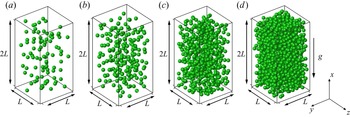
In the present study we focus on modelling of the interfacial terms for the case where the mean slip velocity exists. Thus, we use the DNS data on the particle sedimentation to establish the correlations for the interfacial terms. As shown in figure 1, the particles are freely settling in a periodic cuboid, with the size of $L_{x} \times L_{y} \times L_{z}=2L \times L \times L$. The domain is discretized using a uniform Cartesian grid, and the spatial resolution with respect to the particle size is $d_p/\Delta x = 25.6$. The mean velocity of the suspension in the direction of gravity (i.e. $x$-direction) is kept zero by instantaneously adjusting the pressure gradient.

Figure 1.

Sketches of the particle sedimentation in a fully periodic domain for three different particle volume fractions: (a) $\phi = 2.3\,\%$, (b) $\phi = 5.0\,\%$, (c) $\phi = 14.2\,\%$, (d) $\phi = 30.2\,\%$.

The parameter settings for our simulations are listed in tables 2 and 3. For convenience, we use $\phi$ to denote the particle (or solid) volume fraction. The particle number $N_p$ is given by

(3.21)\begin{equation} N_{p}=\left[\frac{6 \phi}{\rm \pi}\left(\frac{L}{d_{p}}\right)^{3}\right]. \end{equation}

We select four solid volume fractions $\phi =2.3\,\%$, $5.0\,\%$, $14.2\,\%$ and $30.2\,\%$, and two domain sizes: $L/d_p=5$ and 10 for the liquid–solid case of $\rho _r=2.0$, as shown in table 2. We also perform some simulations for $\rho _r=$ 0.01 and 1000, which represent the bubble–liquid and gas–solid systems, respectively, as shown in table 3. Numerical instability was encountered for $\rho _r=$ 0.001 at high particle volume fractions, hence, $\rho _r=$ 0.001 is not considered.

Table 2.

Simulation settings for particles settling in a fully periodic domain at $\rho _r = 2.0$. Here $N_p$ is the total particle number and $\phi$ is the mean solid volume fraction. Because we have two computational domain sizes, the particle numbers before the ‘$/$’ correspond to $L/d_p = 5$ while the numbers after the ‘$/$’ correspond to $L/d_p = 10$.

Table 3.

Simulation settings used for particles settling in a fully periodic domain of $L/d_p = 10$ for various density ratios.

We take the sphere diameter $d_p$ as the characteristic length, and the characteristic velocity $u_c$ is selected as

(3.22)\begin{equation} u_c=\sqrt{\frac{4 d_p}{3}(\rho_{r}-1) g}. \end{equation}

The Galileo number is widely used to measure the particle settling effect, which is defined as

(3.23)\begin{equation} Ga = \frac{{\sqrt {d_p^3( {{\rho _r} - 1} )g} }}{\nu }. \end{equation}

The mean relative (or slip) velocity $u_r$ is defined as the difference between the average solid and fluid-phase velocities directed along the $x$ axis as

(3.24)\begin{equation} {u_r} = \langle {{u_1}} \rangle - \langle {{u_{p,1}}}\rangle. \end{equation}

The particle Reynolds number is defined as $R{e_p} = {u_r}{d_p}/\nu$.

We set $E/(\rho _f u_c^2)=2 \times 10^4$, $\sigma$ = 0.33 and $f = 0.3$ for the collision model. The dimensionless time step is $\Delta t=0.005$ and the statistics are obtained from averaging the data for a duration of 1000 non-dimensional time unit $(d_p/u_c)$ after the statistically steady state is reached. The statistics for the solid-phase velocity and volume fraction are obtained from the data in the solid domain (i.e. inside the particle boundary). Note that we have examined the effects of the box size and the mesh resolution on the results in Appendix A, and ensured that our results are not affected significantly by the box size and the mesh resolution.

4.1. Modelling of dissipation interfacial term

Using the spatial averaging theorem, Schwarzkopf et al. (Reference Schwarzkopf, Crowe and Dutta2009) derived the dissipation rate transport equation of the fluid phase, in which the interfacial terms due to the presence of particles have the form (see also Crowe et al. (Reference Crowe, Schwarzkopf, Sommerfeld and Tsuji2011) for the derivation)

(4.1)\begin{align} {I_\varepsilon } ={-} \frac{{{\rho_f \nu ^2}}}{V}\frac{\partial }{{\partial {x_k}}}\int_{{S_{I}}} {\frac{{\partial {u'_i}}}{{\partial {x_j}}}} \frac{{\partial {u'_i}}}{{\partial {x_j}}}{n_k}\,{\rm d}S + \frac{{2\nu }}{{ V}}\int_{{S_I}} {\frac{{\partial {u'_i}}}{{\partial {x_j}}}} \frac{{\partial p'}}{{\partial {x_j}}}{n_i}\,{\rm d}S - \frac{{{\rho_f \nu ^2}}}{V}\int_{{S_I}} {\frac{\partial }{{\partial {x_k}}}} \left[ {\frac{{\partial {u'_i}}}{{\partial {x_j}}}\frac{{\partial {u'_i}}}{{\partial {x_j}}}} \right]{n_k}\,{\rm d}S. \end{align}

The first and second terms on the right-hand side of (4.1) are not important, as demonstrated by Schwarzkopf et al. (Reference Schwarzkopf, Crowe and Dutta2009). For the Stokes flow in the dilute limit, the last term of (4.1) can be simplified as (Schwarzkopf et al. Reference Schwarzkopf, Crowe and Dutta2009; Crowe et al. Reference Crowe, Schwarzkopf, Sommerfeld and Tsuji2011)

(4.2)\begin{equation} - \frac{{{\rho_f{\nu}^2}}}{V}\int_{{S_I}} {\frac{\partial }{{\partial {x_k}}}} \left( {\frac{{\partial {u'_i}}}{{\partial {x_j}}}\frac{{\partial {u'_i}}}{{\partial {x_j}}}} \right){n_k}\,{\rm d}S = 72{\rm \pi} \frac{{{\rho_f \nu ^2}}}{V}\sum_k {\frac{{{{( {\langle {{u_i}} \rangle - {u_{pki}}} )}^2}}}{{{d_p}}}} = 24\frac{\nu }{{d_p^2}}{I_k}.\end{equation}

The constant ‘24’ can be replaced by the so-called dissipation interfacial term coefficient $C_{\varepsilon 3}$ to account for non-Stokesian effects, resulting in

(4.3)\begin{equation} {I_\varepsilon} = {C_{\varepsilon 3}}\frac{\nu }{{d_p^2}}{I_k}. \end{equation}

Accurate computation of the interfacial term via the integration of (4.2) on the particle surface is difficult for the non-body-fitted approach. Therefore, we quantify it by considering the dissipation rate balance equation (Schwarzkopf et al. Reference Schwarzkopf, Crowe and Dutta2009). For the fully developed homogeneous system with $\mathrm {d} k / \mathrm {d} t = 0$, $\mathrm {d} \varepsilon / \mathrm {d} t=0$ and $\partial \langle {\cdot } \rangle /\partial {x_i} = 0$, the $k$ and $\varepsilon$ equations reduce to

(4.4)$$\begin{gather} {I_k} = \phi_f \rho_f \varepsilon, \end{gather}$$

(4.5)$$\begin{gather}{I_\varepsilon } = {C_{\varepsilon 2}}\phi_f \rho_f \frac{{{\varepsilon ^2}}}{k}. \end{gather}$$

From (4.3)–(4.5), we have

(4.6)\begin{equation} \frac{{{C_{\varepsilon 3}}}}{{{C_{\varepsilon 2}}}} = \frac{{d_p^2}}{\nu }\frac{\varepsilon }{k}. \end{equation}

From (2.21) and (4.4), one can obtain

(4.7)\begin{equation} \varepsilon = \frac{{F_D u_r } }{{\phi _f \rho_f }}.\end{equation}

Substituting (4.7) into (4.6) yields

(4.8)\begin{equation} \frac{{{C_{\varepsilon 3}}}}{{{C_{\varepsilon 2}}}} = \frac{{d_p^2}}{\nu }\frac{1}{{\phi_f \rho_f k}}{F_D}{u_r} = R{e_p}\frac{{{d_p}{F_D}}}{{(1-\phi) \rho_f ({k/u_r^2})u_r^2}}, \end{equation}

which indicates that ${C_{\varepsilon 3}}/{{C}_{\varepsilon 2}}$ is related to the relative TKE $k/u_r^2$ and the mean drag force $F_D$. Hence, to model the interfacial term in the dissipation rate equation, the correlations for the mean drag and the relative TKE are required.

Based on interface-resolved simulations of the flow past fixed random assemblies of monodisperse spheres ($0.1 \le \phi \le 0.5$, $0.01 \le Re_m \le 300$, where $Re_m=(1-\phi )Re_p$), Mehrabadi et al. (Reference Mehrabadi, Tenneti, Garg and Subramaniam2015) proposed the following correlation for the particle-induced relative TKE:

(4.9)\begin{equation} \frac{k}{{u_r^2}} =\phi + 1.25\phi (1 - \phi )^3 \exp (- \phi Re_m^{1/2} ). \end{equation}

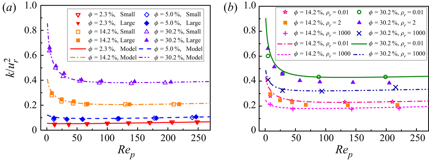
This was shown to be applicable to the dynamic sedimentation system. In the present work we attempt to quantify the relative TKE for the dynamic sedimentation system at different density ratios. Figure 2(a) shows the variation of $k/u_r^2$ with the particle Reynolds number for different solid volume fractions at a density ratio of 2. $k/u_r^2$ for two different box sizes of $L/d_p=10$ and 5, which shows that $k/u_r^2$ slightly increases with increasing domain size. Figure 2(b) shows the effects of the density ratio on $k/u_r^2$ for $\phi =14.2\,\%$ and $30.2\,\%$. From figure 2(a), $k/u_r^2$ decreases rapidly with increasing particle Reynolds number at relatively small $Re_p$, particularly for dense suspensions, consistent with previous simulations of Mehrabadi et al. (Reference Mehrabadi, Tenneti, Garg and Subramaniam2015). For dilute suspensions, we observe a slight increase in $k/u_r^2$ with increasing $Re_p$ at $Re_p > 100$. From figure 2(b), $k/u_r^2$ is higher for a lower density ratio. Using the present DNS data ($0.023 \le \phi \le 0.302$, $Re_p \le 250$) and inspired by the correlation function form of Mehrabadi et al. (Reference Mehrabadi, Tenneti, Garg and Subramaniam2015), a correlation for the relative TKE is obtained as

(4.10)\begin{align} \frac{k}{{u_r^2}} &= 0.92\rho _r^{ - 0.02}{\phi ^{0.78}} + 0.05{\phi ^{0.3}}(1 - \phi ){( {R{e_p}/200} )^{1.1}}\nonumber\\ &\quad + 25{\phi ^2}{( {{\rho _r} + 0.5} )^{ - 0.15}}{(1 - \phi )^3}\exp ( { - {\phi ^{1/2}}{{( {1 - \phi } )}^{1/2}}R{e_p}^{1/2}} ). \end{align}

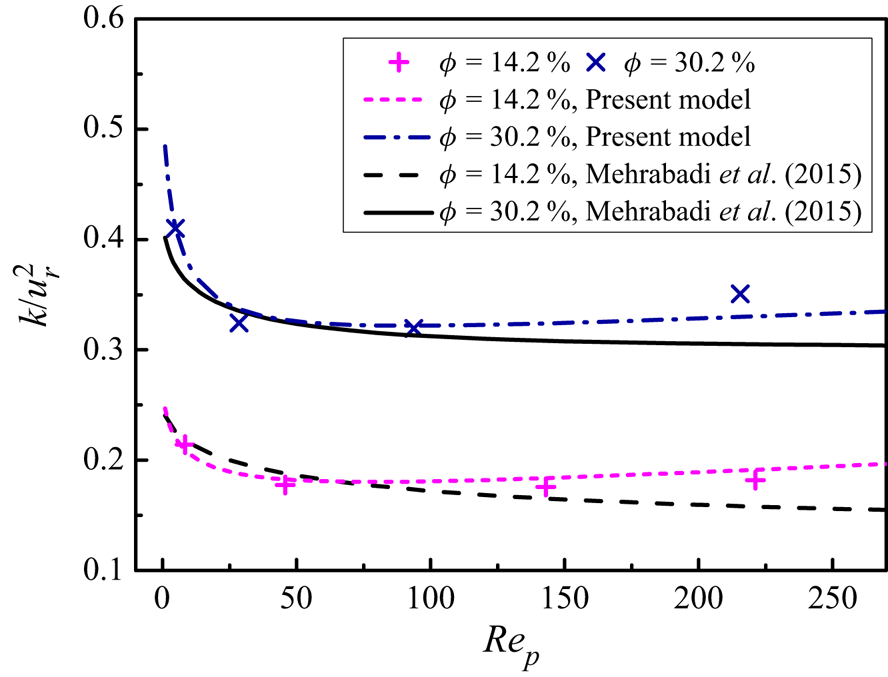
Figure 2 shows that the above correlation agrees well with our DNS data. Figure 3 compares the present correlation of the relative TKE for $\rho _r=1000$ to that of Mehrabadi et al. (Reference Mehrabadi, Tenneti, Garg and Subramaniam2015) obtained from the simulations of fixed spheres. Both correlations are in fairly good agreement with each other. One discrepancy is that the relative TKE of Mehrabadi et al. (Reference Mehrabadi, Tenneti, Garg and Subramaniam2015) decreases monotonically with increasing $Re_p$, whereas ours slightly increases with increasing $Re_p$ for $Re_p > 100$. Mehrabadi et al. 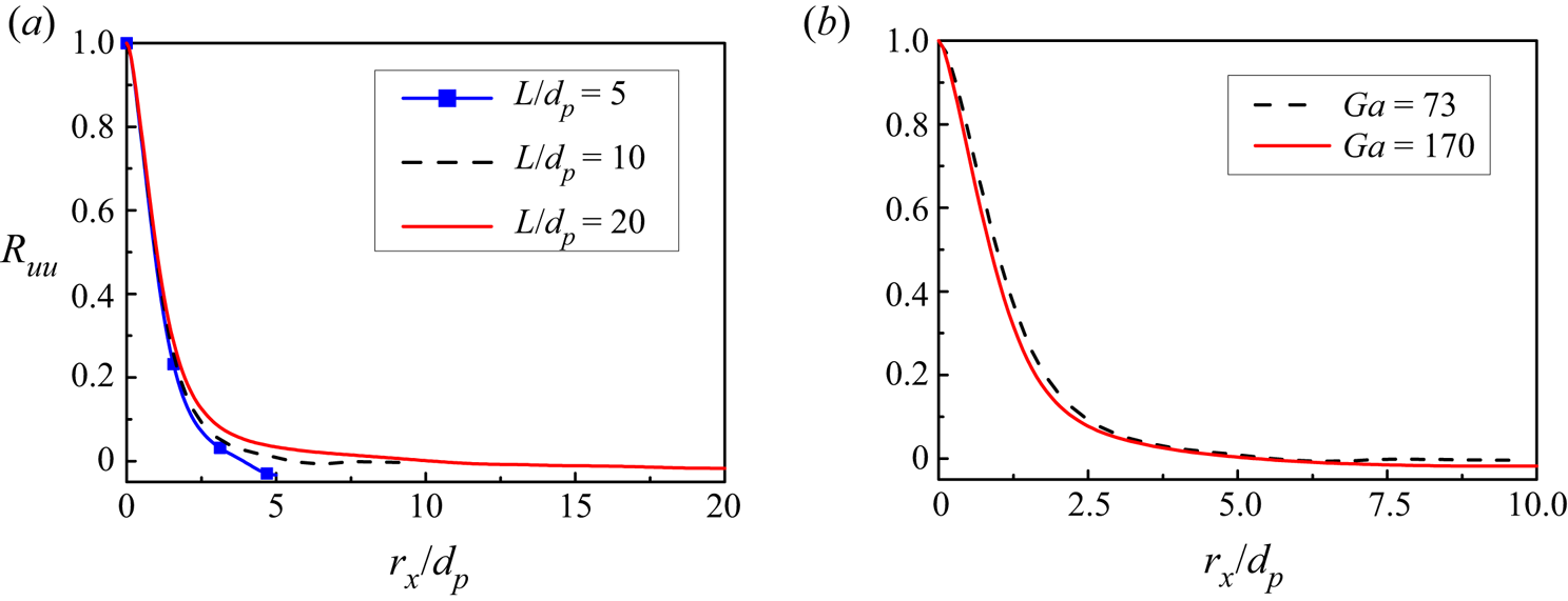(Reference Mehrabadi, Tenneti, Garg and Subramaniam2015) observed that the relative TKE for freely moving particles was slightly greater than that for fixed particles at relatively high $Re_p$. Our computational domain size is larger than that of Mehrabadi et al. (Reference Mehrabadi, Tenneti, Garg and Subramaniam2015), and it has been observed that the relative TKE increases with increasing domain size. Therefore, the differences in the domain size and particle mobility may be responsible for the above discrepancy.

Figure 2.

Relative TKE $k/u_r^2$ as a function of $Re_p$ for (a) $\rho _r = 2.0$ and different domain sizes, and (b) $\rho _r = 0.01$ and 1000 at $L/d_p=10$. The symbols represent the IR-DNS data, while the lines denote the corresponding correlations (4.10). In the legend of (a), ‘small’ represents the smaller domain of $L/d_p = 5$, while ‘large’ represents the larger domain of $L/d_p = 10$.

Figure 3.

Comparison of relative TKE $k/u_r^2$ obtained from the present simulations and from the correlation of Mehrabadi et al. (Reference Mehrabadi, Tenneti, Garg and Subramaniam2015). Our IR-DNS data for $\rho _r = 1000$, denoted by the symbols, and our correlation (4.10), denoted by the lines, are both shown.

We now intend to establish the correlation for the mean drag from our DNS data, which is also required for modelling the dissipation interfacial term (4.8). We take the following form for the drag correlation

(4.11)\begin{equation} {F_D} = \beta u_r,\end{equation}

where $\beta$ is the momentum transfer coefficient.

For $\phi \le 0.1$, we adopt the correlation of $\beta$ obtained in our previous work (Xia et al. Reference Xia, Yu, Pan, Lin and Guo2022b),

(4.12)\begin{equation} \beta_1 = \frac{3}{4}{C_d}\frac{{{\rho _f}\phi (1 - \phi ) {{u_r}}}}{{{d_p}}}{(1 - \phi )^{ - n}}, \end{equation}

where $C_d$ is the modified drag coefficient

(4.13)\begin{equation} C_d=\frac{24}{(1-\phi) R e_{p}}(1+0.15((1-\phi) Re_{p})^{0.687}), \end{equation}

and $n$ is the exponent of the correction function in the form

(4.14)\begin{equation} n=(3.88-0.38 \ln (R e_{p})) \ln (\phi^{{-}1}) \rho_{r}^{{-}0.038}. \end{equation}

For $\phi > 0.1$, based on our DNS data and the modification of the drag correlation of Tang et al. (Reference Tang, Peters, Kuipers, Kriebitzsch and van der Hoef2015) by considering the effects of particle mobility and density ratio, we obtain the following drag correlation:

(4.15)\begin{align} \beta_2 &= 180\frac{{\mu {\phi ^2}}}{{d_p^2(1 - \phi )}} + 18\frac{{{\mu}{{(1 - \phi )}^3}\phi ( {1 + 1.5\sqrt \phi })}}{{d_p^2}}+ \frac{{18\mu \phi (1 - \phi )R{e_m}}}{{d_p^2}}\left[ 0.11\phi ( {1 + \phi } ) \vphantom{\frac{{0.0644}}{{{{(1 - \phi )}^4}}}}\right.\nonumber\\ &\quad -\left. \frac{{0.00456}}{{{{(1 - \phi )}^4}}} +\left( 0.169(1 - \phi )+ \frac{{0.0644}}{{{{(1 - \phi )}^4}}} \right)Re_m^{ - 0.343} \right]\nonumber\\ &\quad + 2.76 Re_m^{0.8}\rho _r^{ - 0.05}\frac{{\mu {\phi ^2}}}{{d_p^2(1 -\phi)}}. \end{align}

We note that in order to avoid the discontinuity of $\beta$ at the critical solid volume fraction (e.g. 0.1 here), Lu et al. (Reference Lu, Gidaspow, Bouillard and Liu2003) proposed a continuous stitching function as $\beta = \kappa {\beta _1} + (1 - \kappa ){\beta _2}$, with $\kappa = \arctan [ {150 \times 1.75(0.1 - \phi )} ]/{\rm \pi} + 0.5$ being an inverse tangent function.

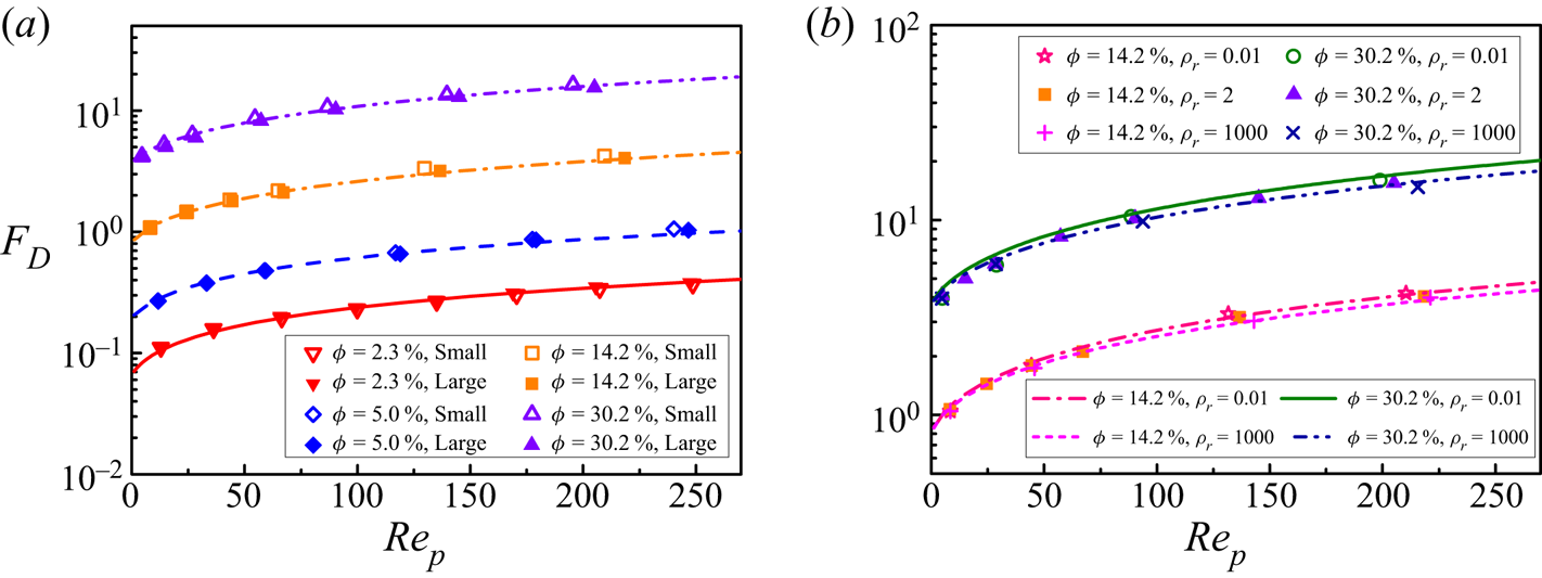
The mean drag forces $F_D$ obtained from IR-DNS normalized with ${3{\rm \pi} \mu (1 - \phi ){d_p}{u_r}/d_p^3}$ at different $Re_p$ and $\phi$ are compared with the present drag correlations in figure 4. The correlations agree well with our DNS data for all cases considered, as shown in figure 4.

Figure 4.

Mean drag forces $F_D$, normalized with ${3{\rm \pi} \mu (1 - \phi ){d_p}{u_r}/d_p^3}$, as a function of $Re_p$ for different $\phi$, and (a) $\rho _r = 2.0$, (b) $\rho _r = 0.01$–1000 and $L/d_p=10$. The symbols denote the IR-DNS data, while the lines present the corresponding drag correlation (4.12) or (4.15). In the legend of (a) , ‘small’ represents the smaller domain of $L/d_p = 5$, while ‘large’ represents the larger domain of $L/d_p = 10$.

With the established correlations for the relative TKE (4.10) and the mean drag coefficient (4.11), the ratio ${C_{\varepsilon 3}}/{{C}_{\varepsilon 2}}$ can be modelled as

(4.16)\begin{equation} \frac{{{C_{\varepsilon 3}}}}{{{C_{\varepsilon 2}}}} = \frac{{\beta R{e_p}}}{{\rho_f(1 - \phi ){{( {k/u_r^2} )}}}}\frac{{{d_p}}}{{{u_r}}}. \end{equation}

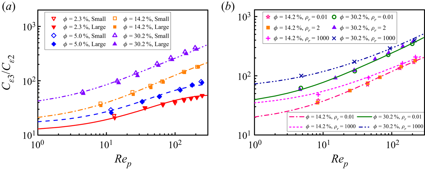
The comparison of this correlation with the IR-DNS data is shown in figure 5. From figure 5(a), ${C_{\varepsilon 3}}/{{C}_{\varepsilon 2}}$ increases with increasing particle Reynolds number or solid volume fraction, when the other parameters are fixed. In addition, the effect of the computational domain size becomes more pronounced at a higher solid volume fraction, and ${C_{\varepsilon 3}}/{{C}_{\varepsilon 2}}$ is larger for a smaller domain size. Figure 5(b) shows that ${C_{\varepsilon 3}}/{{C}_{\varepsilon 2}}$ is much higher for $\rho _r=1000$ than those for $\rho _r=2$ and 0.01, which indicates that the dissipation rate interfacial term is higher for particles with a larger density at the same particle Reynolds number and solid volume fraction.

Figure 5.

Coefficient ratio ${C_{\varepsilon 3}}/{{C}_{\varepsilon 2}}$ as a function of $Re_p$ at different solid volume fractions and (a) $\rho _r = 2.0$, (b) $\rho _r = 0.01$ and 1000, and $L/d_p=10$. The symbols denote the IR-DNS data, while the lines denote the correlation (4.16).

In the dilute limit, $C_{\varepsilon 3}$ can be simplified as

(4.17)\begin{equation} {C_{\varepsilon 3}} = \frac{3}{4}{C_{\varepsilon 2}}\frac{\phi }{{k/u_r^2}}{C_D}R{e_p}. \end{equation}

Therefore, the interfacial term of dissipation rate $I_\varepsilon$ can be expressed as

(4.18)\begin{equation} {I_\varepsilon } = \frac{3}{4}{C_{\varepsilon 2}}\frac{\phi }{{k/u_r^2}}{C_D}R{e_p}\frac{\nu }{{d_p^2}}{I_k} = \frac{3}{4}{C_{\varepsilon 2}}\frac{\phi }{{k/u_r^2}}{C_D}\frac{{{I_k}}}{\tau }, \end{equation}

where $\tau = d_p/u_r$. Our model in the dilute limit (4.18) has a form similar to that of Troshko & Hassan (Reference Troshko and Hassan2001) ($I_\varepsilon = 1.35C_D I_k/\tau$) and Ma et al. (Reference Ma, Santarelli, Ziegenhein, Lucas and Fröhlich2017)($I_\varepsilon = 0.3C_D I_k/\tau$), as shown in table 1.

From (4.8), we have

(4.19)\begin{equation} {\left.{\left[ {(1 - \phi) ( {k/u_r^2} ) \frac{{{C_{\varepsilon 3}}}}{{{C_{\varepsilon 2}}}}} \right]}\right/{\left[ {\frac{{{d_p}{F_D}}}{\rho_f{u_r^2}}} \right]}} = R{e_p}. \end{equation}

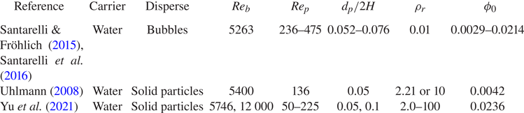
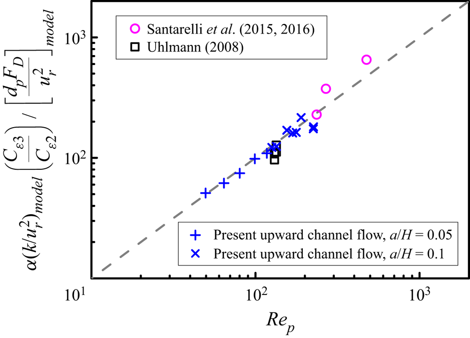
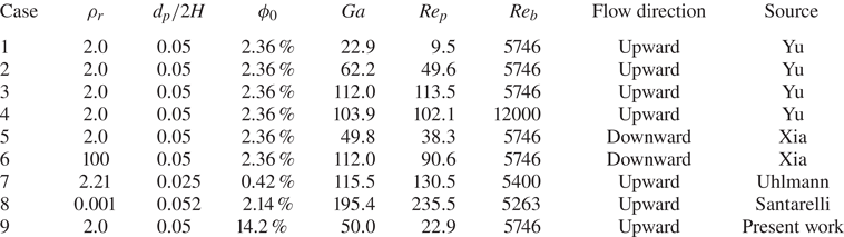
We collect the IR-DNS data on vertical channel flows laden with bubbles or heavy particles in the literature (Uhlmann Reference Uhlmann2008; Santarelli & Fröhlich Reference Santarelli and Fröhlich2015; Santarelli et al. Reference Santarelli, Roussel and Fröhlich2016; Yu et al. Reference Yu, Xia, Guo and Lin2021), as summarized in table 4, and compare them with our model in figure 6. It is noted that the values of ${C_{\varepsilon 3}}/{{C}_{\varepsilon 2}}$ in figure 6 are calculated directly from (4.6), and $F_D$ and ${k/u_r^2}$ are computed with our correlations (4.10) and (4.11). All data are collected in the sedimentation-dominated regime of $\sqrt k /{u_r} \ll 1$ at the channel centre. Our model agrees very well with the DNS data of Yu et al. (Reference Yu, Xia, Guo and Lin2021) for particle Reynolds numbers below 200, and is in fairly good agreement with those of Uhlmann (Reference Uhlmann2008), Santarelli & Fröhlich (Reference Santarelli and Fröhlich2015) and Santarelli et al. (Reference Santarelli, Roussel and Fröhlich2016).

Table 4.

Summary of the previous works on interface-resolved simulations of vertical turbulent particle-laden channel flows.

Figure 6.

Previous IR-DNS data on ${C_{\varepsilon 3}}/{{C}_{\varepsilon 2}}$ at the channel centre for vertical channel flows, as compared with the model (4.19).

4.2. Modelling of the interfacial term in Reynolds stress equation

The presence of particles gives rise to strong anisotropy for the Reynolds stress transport. For the homogeneous sedimentation system at steady state, the Reynolds stress equations (2.4) reduce to

(4.20)\begin{equation} {\varPhi_{ij}} - {\varepsilon_{ij}} + {I_{ij}} = 0. \end{equation}

Considerable efforts have been devoted to the modelling of the dissipation rate tensor ${\varepsilon _{ij}}$, pressure–strain term ${\varPhi _{ij}}$ and interfacial term ${I_{ij}}$.

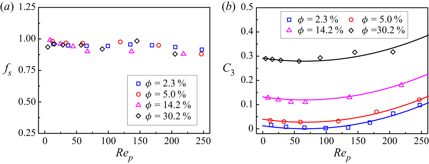
Poelma, Westerweel & Ooms (Reference Poelma, Westerweel and Ooms2007) have demonstrated experimentally that relative motion between the phases induced by gravity forces can lead to significant anisotropy in the fluid-phase dissipation tensor ${\varepsilon _{ij}}$. Using the present DNS data, we determine the coefficient $f_s$ in (2.8), and the results for different $Re_p$ and $\phi$ at $\rho _r=2.0$ are plotted in figure 7(a). Baker et al. (Reference Baker, Fox, Kong, Capecelatro and Desjardins2020) adopted $f_s=0.9$. Figure 7(a) shows that $f_s$ from our DNS data is insensitive to the variation of $Re_p$ and $\phi$, and $f_s=0.9$ is a good choice. It should be noted that the results for $\rho _r=0.01$ and 1000 are similar to those for $\rho _r=2.0$ in figure 7(a), but are not shown here for clarity.

Figure 7.

Plots of (a) $f_s$ and (b) $C_3$ as a function of $Re_p$ for different solid volume fractions and $\rho _r=2$. The symbols denote our IR-DNS data, and the solid lines represent the model (4.22).

For the homogeneous sedimentation system, the pressure–strain term ${\varPhi _{ij}}$ reduces to

(4.21)\begin{equation} {\varPhi_{ij}} ={-} \phi_f \rho_f {C_1}\varepsilon {a_{ij}} + \phi_f \rho_f{C'_1}\varepsilon ( {{a_{ik}}{a_{kj}} - \tfrac{1}{3}{A_2}{\delta _{ij}}} ) - {C_3}( {{I_{ij}} - \tfrac{1}{3}{\delta _{ij}}{I_{kk}}} ). \end{equation}

With the standard coefficients $C_1=1.7$ and $C'_1=1.05$ for the SSG model (Hanjalić & Launder Reference Hanjalić and Launder2011), the only unknown coefficient $C_3$ can be obtained using the DNS data from (4.21). The results are shown in figure 7(b). Obviously, $C_3$ increases with increasing $\phi$. For dilute flows ($\phi = 2.3\,\%$) at $Re_p < 150$, $C_3$ is almost zero. For $\rho _r=2$, $C_3$ is a function of particle volume fraction and particle Reynolds number in the form

(4.22)\begin{equation} {C_3}( {\phi ,R{e_p}} ) = \phi + aR{e_p} + bRe_p^2 + c,\end{equation}

in which $a=3.723 \times 10^{-4}$, $b=2.819 \times 10^{-6}$ and $c=-0.010$. The correlation of ${C_3}$ (4.22) is compared with the DNS data in figure 7(b), and good agreement can be observed. We note that $C_3$ is not sensitive to the variation of the density ratio from our DNS (not shown here), thus, the correlation (4.22) is applicable to other density ratios.

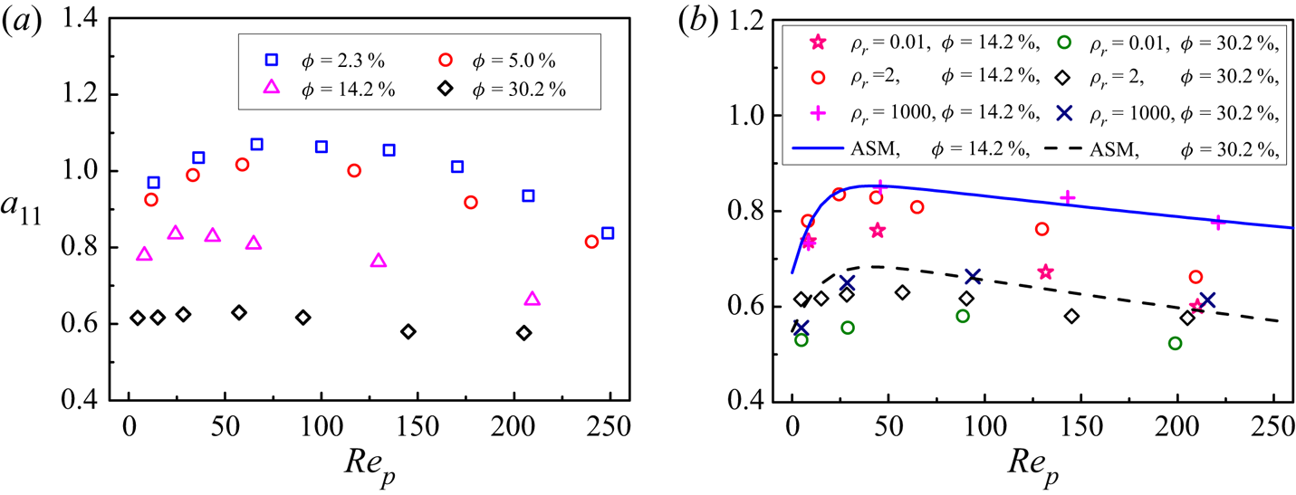
The non-monotonic trend of $C_3$ with $Re_p$ may be related to the particle-induced fluid Reynolds stress anisotropy $a_{ij}$ defined by (2.14), since $C_3$ is determined from (4.21) with the DNS data of $a_{ij}$, $\varPhi _{ij}$ and $I_{ij}$. Our results on the Reynolds stress anisotropy component in the vertical direction $a_{11}$ are shown in figure 8. From figure 8, $a_{11}$ increases with increasing $Re_p$ at relatively low $Re_p$, and then decreases with increasing $Re_p$ above a critical $Re_p$, being opposite to the dependence of $C_3$ on $Re_p$, as shown in figure 7(b). From figure 8, $a_{11}$ decreases with increasing $\phi$, which indicates that the anisotropy of the velocity fluctuation decreases with increasing $\phi$, since $a_{11}+a_{22}+a_{33}=2$ and $a_{22} = a_{33}$. Mehrabadi et al. (Reference Mehrabadi, Tenneti, Garg and Subramaniam2015) argued that the magnitude of anisotropy is determined by the ratio of the length of elongated structures to the inter-particle spacing (Mehrabadi et al. Reference Mehrabadi, Tenneti, Garg and Subramaniam2015). In addition, figure 8(b) shows that $a_{11}$ increases with increasing density ratio, particularly for high $Re_p$, and $a_{11}$ for $\rho _r=1000$ is in good agreement with the algebraic stress model proposed by Mehrabadi et al. (Reference Mehrabadi, Tenneti, Garg and Subramaniam2015) obtained from the DNS data for fixed spheres, which provides evidence for good accuracy of our DNS data.

Figure 8.

Reynolds stress anisotropy component $a_{11}$ for different $Re_p$ and $\phi$ at (a) $\rho _r = 2.0$ and (b) $\rho _r = 0.01$–1000. The symbols denote our IR-DNS data, while the lines represent the model proposed by Mehrabadi et al. (Reference Mehrabadi, Tenneti, Garg and Subramaniam2015) from DNS of fixed particles.

The force term $\varPhi _{ij,3}$ with the coefficient of $C_3$ in the pressure–strain model is caused by the presence of particles, and this term can be combined with the interfacial term $I_{ij}$. Ma et al. (Reference Ma, Lucas, Jakirlić and Fröhlich2020b) defined an effective particle-induced interfacial term $I_{ij}^{*} = {\varPhi _{ij,3}} + {I_{ij}}$, i.e.

(4.23)\begin{equation} I_{ij}^* = {b_{ij}}{I_k} - {C_3}( {{I_{ij}} - \tfrac{1}{3}{\delta _{ij}}{I_{kk}}} ) = [ {( {1 - {C_3}} ){b_{ij}} + \tfrac{2}{3}{C_3}{\delta _{ij}}} ]{I_k}. \end{equation}

Therefore, we have $I_{ij}^* = {b_{ij}^*}{I_k}$, with

(4.24)\begin{equation} {b_{ij}^*} = {( {1 - {C_3}} ){b_{ij}} + \tfrac{2}{3}{C_3}{\delta _{ij}}}. \end{equation}

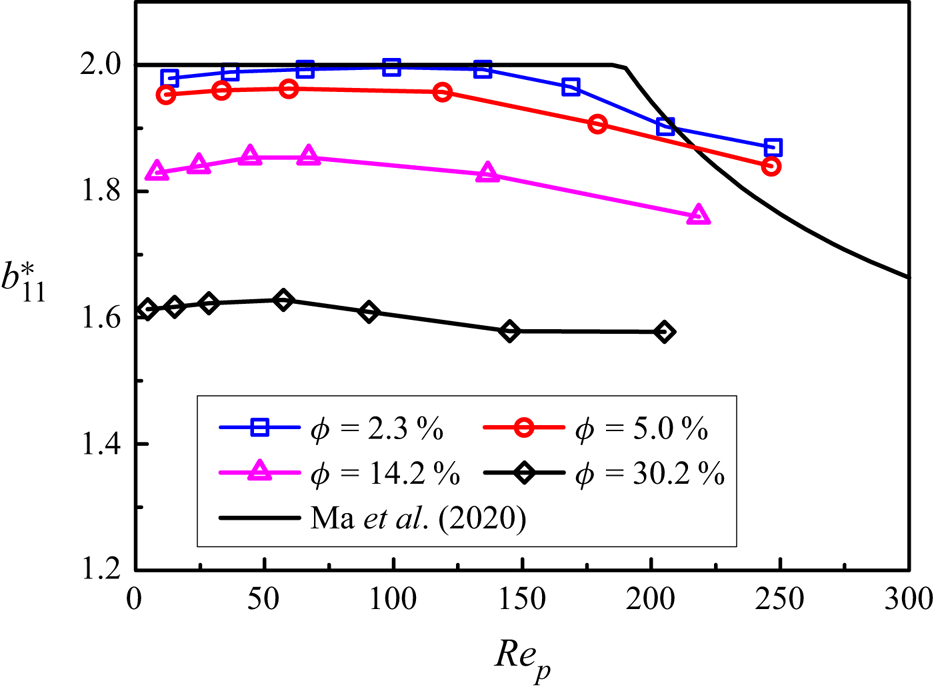
As discussed in § 2, $b_{11}=2.0$ and $b_{22}=b_{33}=0$, if the mean slip velocity exists only in one direction. Figure 9 shows $b_{11}^{*}$ as a function of $Re_p$ for different $\phi$ at $\rho _r=2$. Clearly, $b_{11}^{*}$ decreases with increasing $\phi$, as $a_{11}$ in figure 8, which indicates a trend towards stronger isotropy at a higher $\phi$. For $\phi = 2.3\,\%$ and $Re_p < 150$, our $b_{11}^{*}$ is close to 2.0, which is consistent with the correlation of Ma et al. (Reference Ma, Lucas, Jakirlić and Fröhlich2020b) from DNS of bubbly flows at relatively low particle volume fractions and high particle Reynolds numbers: $b_{11}^{*} = \min (0.67+0.67 \exp (370 R e_{p}^{-1.2}), 2)$ (Ma et al. Reference Ma, Lucas, Jakirlić and Fröhlich2020b).

Figure 9.

Modified interfacial term $b_{11}^*$ as a function of $Re_p$ for different $\phi$ at $\rho _r=2$. The solid line represents the correlation of Ma et al. (Reference Ma, Lucas, Jakirlić and Fröhlich2020b).

5.1. Near-wall RSM for particle-laden turbulent channel flows

Most turbulence models were developed for high Reynolds numbers, and they are not suitable for low-$Re$ wall-bounded channel flows where the viscous effects permeate the whole region. The Reynolds numbers for all IR-DNS data available are low, hence, the near-wall Reynolds stress model (So et al. Reference So, Aksoy, Yuan and Sommer1996) for the single-phase turbulent flows is employed. In the present study we assume that the presence of particles do not affect the model parameters existing in the single-phase case in (2.4) and (2.23), and we only supplement with the particle-induced terms.

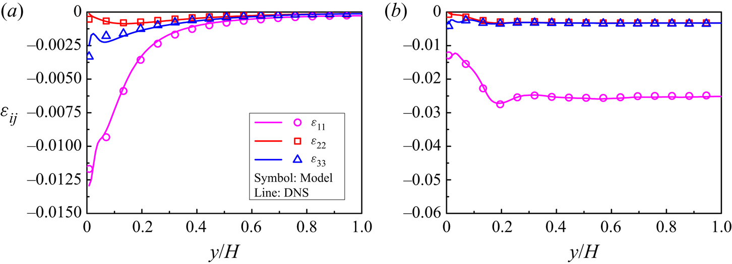
For the dissipation term, the model (2.8) is employed with $f_s=0.9$, as discussed earlier in association with figure 7(a). The components of the dissipation term $\varepsilon _{ij}$ predicted by the model (2.8) using the DNS data of the dissipation rate $\varepsilon$ and Reynolds stresses are compared with the DNS data of $\varepsilon _{ij}$ for the typical cases (cases 1 and 3) in figure 10. Remarkably good agreement can be seen, which indicates that the anisotropic model (2.8) with $f_s=0.9$ is suitable for the particle-laden channel flow.

Figure 10.

Comparison between the dissipation rate tensor $\varepsilon _{ij}$ obtained fully from the DNS simulations and from the model (2.8) with $f_s=0.9$ and the DNS data of the dissipation rate $\varepsilon$ for (a) case 1 ($Re_p=9.5$) and (b) case 3 ($Re_p=113.5$). All values are normalized with $\rho _{f} u_{b}^{3} / H$.

From (2.10)–(2.13), the pressure–strain tensor $\varPhi _{ij}$ for turbulent channel flows reads

(5.1)\begin{align} {\varPhi _{ij}} &={-} \phi_f \rho_f ( {{C_1}\varepsilon + C_1^*{P_k}} ){a_{ij}} + \phi_f \rho_f{C'_1}\varepsilon ( {{a_{ik}}{a_{kj}} - \tfrac{1}{3}{A_2}{\delta _{ij}}} )\nonumber\\ &\quad - \phi_f\rho_f{C_2}({{P_{ij}} - \tfrac{2}{3}{P_k}{\delta _{ij}}} ) - \phi_f \rho_f{C_4}( {{E_{ij}} - \tfrac{2}{3}{P_k}{\delta _{ij}}} )\nonumber\\ &\quad -\phi_f \rho_f (0.033+0.65A_2^{1/2})k{S_{ij}} - {C_3}( {{I_{ij}} - \tfrac{1}{3}{\delta _{ij}}{I_{kk}}} ) + \varPhi_{ij}^w. \end{align}

Here the near-wall correction tensor $\varPhi _{ij}^w$ is given by So et al. (Reference So, Aksoy, Yuan and Sommer1996)

(5.2)\begin{align} \varPhi_{ij}^w = {f_{w}}\phi_f \rho_f [ {( {{C_1}\varepsilon + C_1^*{P_k}} ){a_{ij}} - {C'_1}\varepsilon ( {{a_{ik}}{a_{kj}} - \tfrac{1}{3}{A_2}{\delta _{ij}}} ) + {\alpha^*}( {{P_{ij}} - \tfrac{2}{3}{P_k}{\delta _{ij}}} ) + 2{\gamma ^*}k{S_{ij}}} ], \end{align}

where $f_{w}$ is a damping function given as $f_{w}=\exp [-(\operatorname {Re}_{t} / 200)^{2}]$, with $Re_t$ being the turbulent Reynolds number $R{e_t} = {k^2}/\varepsilon \nu$. Here $\alpha ^{*}$ and $\gamma ^{*}$ are constants in the SSG model, which can provide a better prediction for a fully developed channel flow in the near-wall region.

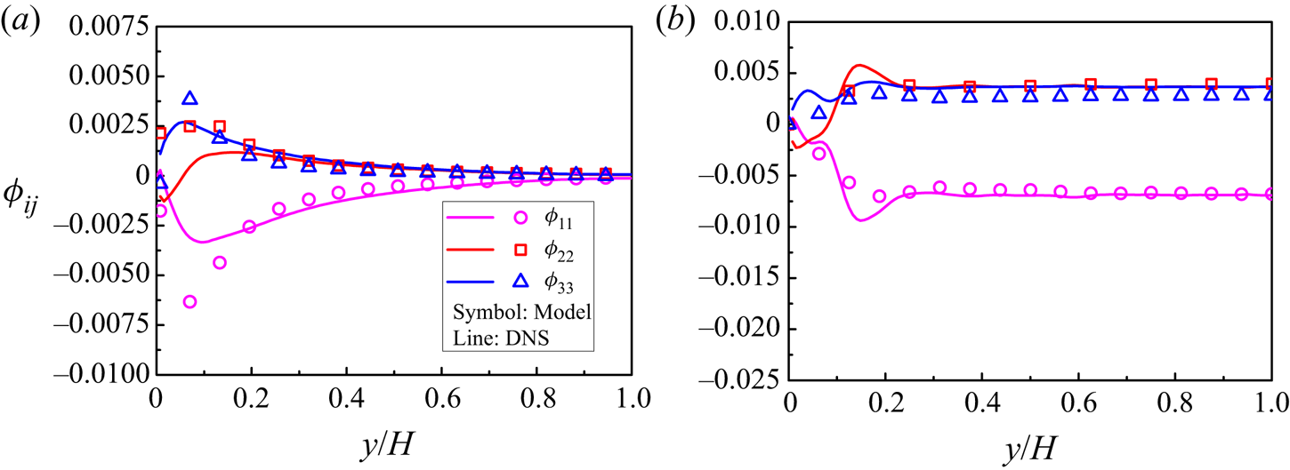
Comparison between the pressure–strain terms obtained directly from (2.9) and from the model (5.1) using the DNS data for cases 1 and 3 is shown in figure 11. The model predicts well the pressure–strain term for both shear-induced turbulence and particle-induced turbulence in the bulk region, but the accuracy of the model is not good in the near-wall region. It is a difficult issue how to accurately model the pressure–strain term in the near-wall region for low-$Re$ wall-bounded flows even for the single-phase case.

Figure 11.

Comparison between the pressure–strain terms $\varPhi _{ij}$ obtained directly from (2.9) and from the model (5.1) using the DNS data for (a) ($Re_p=9.5$) and (b) case 3 ($Re_p=113.5$). All values are normalized with $\rho _{f} u_{b}^{3} / H$.

In the modelled $\varepsilon$ equation, to account for near-wall effects, the term ${\varepsilon _\varepsilon }$ is modified as

(5.3)\begin{equation} {\varepsilon _\varepsilon } = {C_{\varepsilon 2}}\phi_f \rho_f \frac{{\varepsilon \tilde \varepsilon }}{k}, \end{equation}

where $\tilde \varepsilon = \varepsilon - 2\nu {(\sqrt k /y)^2}$, with $y$ being the normal distance from the wall. The difference between $\tilde \varepsilon$ and $\varepsilon$ disappears at the edge of the viscous region for the low-Reynolds-number case (e.g. $Re_{\tau }=180$) (Hanjalić & Launder Reference Hanjalić and Launder2011).

5.2. Comparison between RANS and DNS

We consider vertical channel flows, with gravity points downwards. We define the streamwise, wall-normal and spanwise directions as $x$, $y$ and $z$, respectively, and also as $x_1$, $x_2$ and $x_3$, respectively. For fully developed channel flows, we have ${\langle {{u'_3}{u'_1}} \rangle = \langle {{u'_3}{u'_2}} \rangle = 0}$, ${\langle {{u_2}} \rangle = \langle {{u_3}} \rangle = 0}$ and $\partial \langle {{u_1}} \rangle /\partial {x_1} = \partial \langle {{u_1}} \rangle /\partial {x_3} = 0$. Thus, the dimensionless volume-averaged equations for the fluid phase can be simplified as

(5.4)\begin{equation} \left. \begin{array}{c@{}} {\dfrac{{\partial \phi_f \langle {{u_1}} \rangle }}{{\partial t}} ={-} \phi_f \dfrac{{{\rm d} \langle p \rangle }}{{{\rm d} {x_1}}} + \dfrac{1}{Re}\dfrac{\partial }{{\partial x_2}}(\phi_f \dfrac{{\partial \langle {{u_1}} \rangle }}{{\partial x_2}}) - \dfrac{{\partial ( {\phi_f \langle {{u'_1}{u'_2}} \rangle } )}}{{\partial x_2}} - F_D }, \\ {\dfrac{{\partial \phi_f \langle {{u'_1}{u'_1}} \rangle }}{{\partial t}} ={-} 2\phi_f \langle {{u'_1}{u'_2}} \rangle \dfrac{{\partial \langle {{u_1}} \rangle }}{{\partial x_2}} + {D_{11}} + {\varPhi _{11}} + {\varepsilon _{11}} + {I_{11}}}, \\ {\dfrac{{\partial \phi_f \langle {{u'_2}{u'_2}} \rangle }}{{\partial t}} = {D_{22}} + {\varPhi _{22}} + {\varepsilon _{22}} +{I_{22}}}, \\ {\dfrac{{\partial \phi_f \langle {{u'_3}{u'_3}} \rangle }}{{\partial t}} = {D_{33}} + {\varPhi _{33}} + {\varepsilon _{33}} + {I_{33}}}, \\ {\dfrac{{\partial \phi_f \langle {{u'_1}{u'_2}} \rangle }}{{\partial t}} ={-} { \phi_f \langle {{u'_2}{u'_2}} \rangle \dfrac{{\partial \langle {{u_1}} \rangle }}{{\partial {x_2}}}} + {D_{12}} + {\varPhi _{12}} + {\varepsilon _{12}} + {I_{12}}}, \\ {\dfrac{{\partial \phi_f \varepsilon }}{{\partial t}} = {P_\varepsilon } + {D_\varepsilon } + {\varepsilon _\varepsilon } + {I_\varepsilon }}. \end{array} \right\} \end{equation}

The pressure gradient is determined from the constraint that the flow rate (or bulk velocity) is constant. The following boundary conditions are imposed on the wall: $\langle {u_i} \rangle =0$, $\langle {u'_i u'_j} \rangle =0$ and $\varepsilon = 2\nu {( {\textrm {d}\sqrt k /\textrm {d}x_2} )^2}$. Equations (5.4) are solved with an in-house code using a time advancement scheme to achieve the steady-state solution.

The full two-fluid RSM is complex (Fox Reference Fox2014; Baker et al. Reference Baker, Fox, Kong, Capecelatro and Desjardins2020), involving some sub-models for the solid phase, such as the lift model and the particle stress model. In order to evaluate the performance of the interfacial term models proposed in the present study, the uncertainty from other models should be minimized. Therefore, inspired by the work of Ma et al. (Reference Ma, Lucas, Jakirlić and Fröhlich2020b), we only solve the fluid-phase transport equations (5.4), and directly use the DNS data for the solid-phase quantities involved in the fluid equations, such as the particle volume fraction, the mean slip velocity and the mean drag. Table 6 presents the empirical coefficients in our RANS simulations.

Table 6.

Coefficients in the present RANS simulations of particle-laden channel flows.

The DNS mean drag is obtained from the fluid mean momentum equation in the dimensional form at statistically steady state

(5.5)\begin{equation} {F_D} = \frac{{\rm d}}{{{\rm d}{x_2}}}\left( {{\phi _f}\mu \frac{{{\rm d}\langle {{u_1}} \rangle }}{{{\rm d}{{x}_{{2}}}}}} \right) + {\phi _f}\left( { - \frac{{{\rm d}{p_e}}}{{{\rm d}{x_1}}}} \right) + \frac{{\rm d}}{{{\rm d}{x_2}}}( {{\phi _f}{\rho _f}\langle { - {u'_1}{u'_2}} \rangle } ). \end{equation}

From the domain-averaged momentum balance for the mixture, the mean pressure gradient $-\mathrm {d} p_{e} / \mathrm {d} x=\tau _{w} / H+\phi _{0}(\rho _{s}-\rho _{f}) g$ for upward flow, while $-\mathrm {d} p_{e} / \mathrm {d} x=\tau _{w} / H-\phi _{0}(\rho _{s}-\rho _{f}) g$ for downward flow.

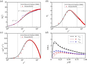
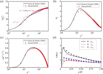
To evaluate the performance of the original near-wall RSM for the single-phase flow, we compare the results on the single-phase turbulent channel flow from the model with the DNS results of Hoyas & Jiménez (Reference Hoyas and Jiménez2008) in Appendix B. It is shown that the model can predict well the turbulence statistics, which lays a foundation for the application of the RSM to particle-laden flows.

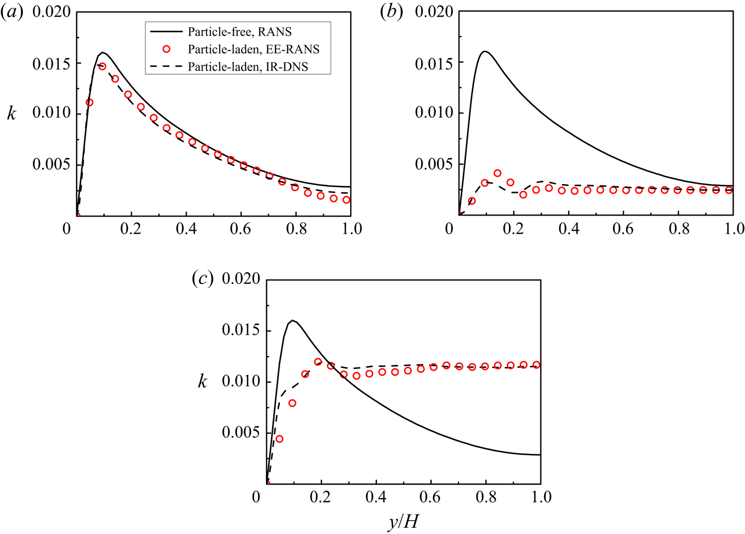
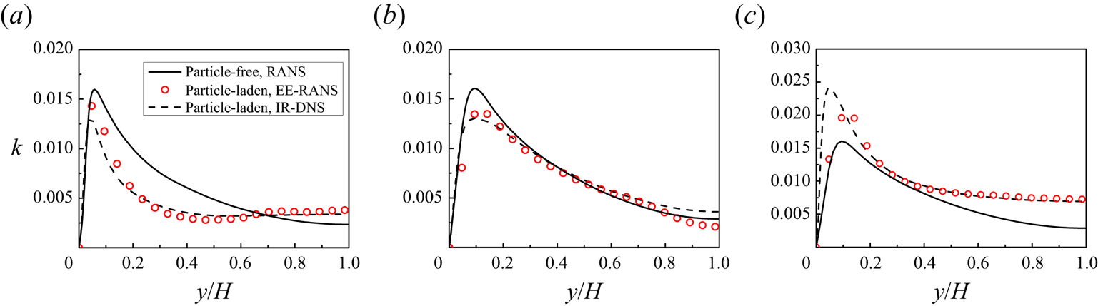
The results on TKE from the RANS simulations of upward particle-laden turbulent channel flows for cases 1–3 in table 5 are compared with the DNS results of Yu et al. (Reference Yu, Xia, Guo and Lin2021) in figure 12. Turbulence suppression across the entire channel is observed for cases 1 ($Re_p=9.5$) and 2 ($Re_p=49.6$), whereas turbulence augmentation in the bulk region takes place for case 3 ($Re_p=113.5$). The RANS results agree well with the DNS results, as shown in figure 12. To the best of our knowledge, this is the first demonstration of using RANS simulations to well predict particle-induced turbulence enhancement and attenuation in vertical channel flows.

Figure 12.

Profiles of TKE for (a) case 1 (upflow, $Re_p=9.5$), (b) case 2 (upflow, $Re_p=49.6$), (c) case 3 (upflow, $Re_p=113.5$).

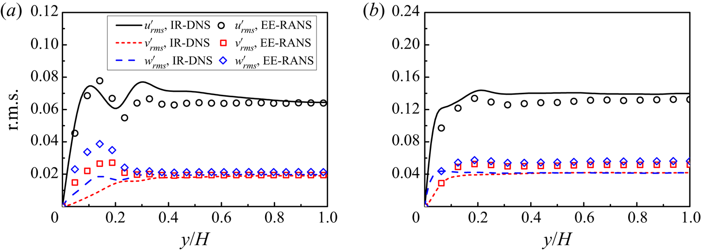
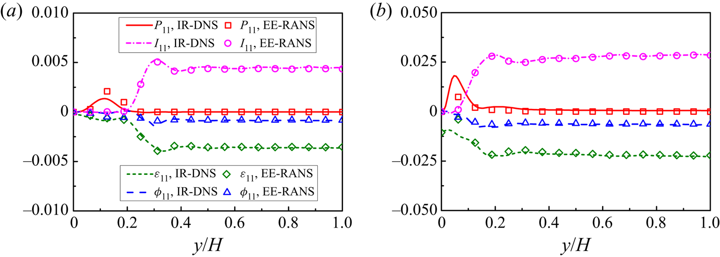
Figures 13 and 14 show that the root-mean-square (r.m.s.) values of the fluid velocity fluctuations and some selected terms in the Reynolds stress equation of $\langle u'_1u'_1 \rangle$ from RANS agree well with the DNS results, which indicate that the particle-induced anisotropy is correctly captured by our RSM. Nevertheless, significant over-estimation of $v'_{rms}$ and $w'_{rms}$ near the wall by the RANS simulations can be observed in figure 13(a). We note that such over-prediction occurs for the RANS simulation of the single-phase flow, as shown in figure 22. In addition, figure 13 shows that the discrepancy of wall-normal and spanwise r.m.s. velocities between Euler–Euler RANS and IR-DNS becomes relatively larger in the centre region of the channel at a higher particle Reynolds number, which is a surprising result, since one may assume that the flow tends to become a more homogeneous sedimentation system as the particle Reynolds number increases. From our previous study (Yu et al. Reference Yu, Xia, Guo and Lin2021), the shear turbulence (characterized by the Reynolds shear stress) in an upward channel flow can be attenuated by the settling particles, however, the effect is non-monotonic with increasing particle Reynolds number. Above the critical $Re_p$, the Reynolds shear stress increases with increasing $Re_p$ (see also figure 16), which may indicate that the flow deviates more from the homogeneous sedimentation system at a higher $Re_p$. Our models for the interfacial terms are based on the data of the homogeneous sedimentation in a periodic domain, and we conjecture that this is the reason why the discrepancy in the channel bulk region is higher for $Re_p$=113.5 than that for $Re_p$=49.6 in figure 13. We note that there is also a more pronounced discrepancy in the Reynolds shear stress for $Re_p$=113.5 (figure 16). We leave the improvement of the model in the presence of shear turbulence effects for the near-wall region and the r.m.s.velocities in the bulk region to a future study.

Figure 13.

Root-mean-square velocity components from RANS and DNS for (a) case 2 ($Re_p=49.6$) and (b) case 3 ($Re_p=113.5$).

Figure 14.

Comparison between RANS and DNS on the selected terms in the equation of $< u'_1u'_1>$ for (a) Case 2 ($Re_p=49.6$), and (b) Case 3 ($Re_p=113.5$). All terms are normalized with $\rho _{f} u_{b}^{3} / H$.

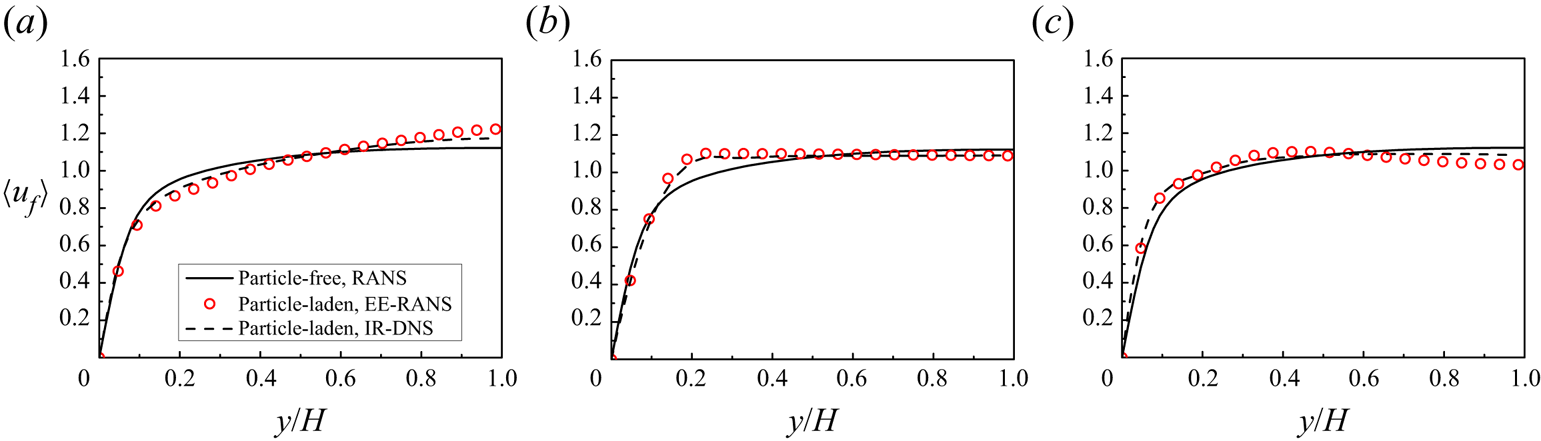
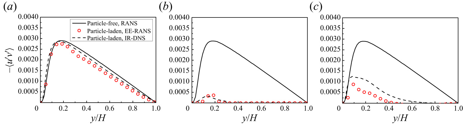
From figures 15 and 16, the fluid mean velocities and Reynolds shear stress from the RANS model also agree well with the DNS results. As $Re_p$ increases from 9.5 to 49.6, the mean velocity profile becomes flatter and the Reynolds shear stress becomes much smaller, which are well captured by the RANS simulations.

Figure 15.

Mean fluid velocity profiles of turbulent channel flows for (a) case 1 (upflow, $Re_p=9.5$), (b) case 2 (upflow, $Re_p=49.6$) and (c) case 3 (upflow, $Re_p=113.5$).

Figure 16.

Reynolds shear stress $-\langle u^{\prime } v^{\prime }\rangle$ profiles for (a) case 1 (upflow, $Re_p=9.5$), (b) case 2 (upflow, $Re_p=49.6$) and (c) case 3 (upflow, $Re_p=113.5$).

The profiles of TKE for cases 4–6 in table 5 are shown in figure 17. The results show that the RSM also works well for the situations of higher flow Reynolds number, downward flow and high density ratio. Particularly, figures 12(b) and 17(b) indicate that the effects of flow direction on TKE can be captured by the RANS model: from figure 12(b), for upflow at $Re_p=49.6$ (case 2), the turbulence is significantly suppressed by particles, whereas from figure 17(b), for downflow at $Re_p=38.3$ (case 5), the turbulence is roughly not attenuated by particles, particularly if compared with the DNS result of the single-phase flow (Xia et al. Reference Xia, Lin, Pan and Yu2021). Xia et al. (Reference Xia, Lin, Pan and Yu2021) attributed the reason for the difference to the observations that, for case 2, the particles migrate towards the channel centre, and the shear-induced large-scale vortices are significantly suppressed, whereas, for case 5, the particles migrate towards the channel wall, and the flow is still dominated by large-scale vortices. It is interesting that the RANS simulation does not resolve the vortices, but is able to predict the turbulence attenuation or enhancement quantitatively.

Figure 17.

Comparison of the TKE profile predicted by RANS and DNS for (a) case 4 (upflow, $Re_p$=102.1, $Re_b=12000$), (b) case 5 (downflow, $Re_p$=38.3) and (c) case 6 (downflow, $\rho _r=100$, $Re_p$=90.6).

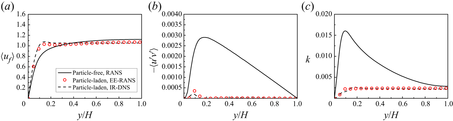
The profiles of mean fluid velocity, Reynolds shear stress $-\langle u^{\prime } v^{\prime }\rangle$, as well as TKE for case 9 ($\phi _{0}=14.2\,\%$, $Re_p$=22.9) in table 5 are shown in figure 18. The results show that our model prediction is still good for larger volume fractions. We note that in the bulk region the shear turbulence is almost completely suppressed by the particles in this case ($\phi _{0}=14.2\,\%,Re_p=22.9$), evidenced by vanishingly small Reynolds shear stress.

Figure 18.

(a) Mean fluid velocity, (b) Reynolds shear stress $-\langle u^{\prime } v^{\prime }\rangle$ and (c) TKE profiles predicted for case 9 ($\phi _{0}=14.2\,\%, Re_p=22.9$).

In the following we attempt to identify the main reason why the appreciable turbulence attenuation occurs in the RANS simulations for case 2, but not for case 5. Vreman (Reference Vreman2015) demonstrated that the non-uniform part of the drag force contributed significantly to the particle-induced turbulence attenuation in point-particle simulations. The same analysis method is used here, with a minor difference that the effect of the particle volume fraction is taken into account, which was not considered by Vreman (Reference Vreman2015) for point-particle simulations.

The domain-averaged mean momentum equation of the fluid phase can be derived from (5.5) as

(5.6)\begin{equation} - \frac{{\tau _w } }{H} + \overline{\phi_{f}} \left( { - \frac{{{\rm d}p_e } }{{{\rm d}x_1 }}} \right) - \overline{F_D } = 0,\end{equation}

where $\overline {\phi _{f}}$ and $\overline {F_{D}}$ are the domain-averaged fluid volume fraction and drag force. If this equation is subtracted from (5.5), we obtain

(5.7)\begin{equation} \frac{\mathrm{d}}{\mathrm{d} x_{2}}\left(\phi_{f} \mu \frac{\partial\langle u_{1}\rangle}{\partial x_{2}}\right)+\phi_{f}^{nu}\left(-\frac{\mathrm{d} p_{e}}{\mathrm{d} x_{1}}\right)+\frac{\mathrm{d}(\phi_{f} \rho_{f}\langle-u_{1}^{\prime} u_{2}^{\prime}\rangle)}{\mathrm{d} x_{2}}+\frac{\tau_{w}}{H}-F_{D}^{nu}=0, \end{equation}

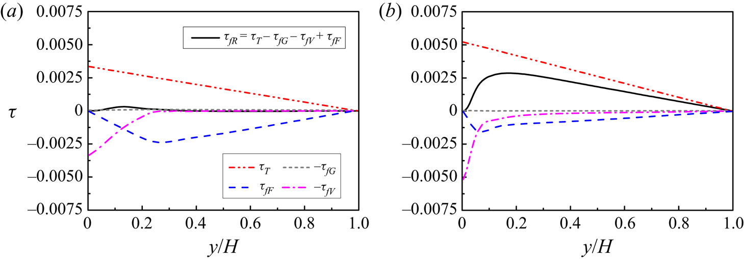
where $F_{D}^{nu}$ and $\phi _{f}^{nu}$ are the non-uniform part of the drag and the fluid volume fraction, respectively, i.e. $F_{D}^{nu}=F_{D}-\overline {F_{D}}$ and $\phi _{f}^{nu}=\phi _{f}-\overline {\phi _{f}}$. Integrating (5.7) from the wall ($x_2=0$) to $x_2=y$, we obtain

(5.8)\begin{align} \underbrace{(\phi_{f} \rho_{f}\langle-u_{1}^{\prime} u_{2}^{\prime}\rangle)}_{\tau_{f R}} &=\underbrace{\tau_w \left(1-\frac{y}{H}-\frac{\displaystyle \int_{0}^{y} \phi_{f}^{n u}\, \mathrm{d} x_{2}}{H}\right)}_{\tau_{T}} \mp \underbrace{\phi_0 (\rho_{s}-\rho_{f}) g \int_{0}^{y} \phi_{f}^{n u}\, \mathrm{d} x_{2}}_{\tau_{G}} \nonumber\\ & \quad -\underbrace{\left(\phi_{f} \mu \frac{\partial\langle u_{1}\rangle}{\partial x_{2}}\right)}_{\tau_{fV}}+\underbrace{\int_{0}^{y} F_{D}^{nu}\, \mathrm{d} x_{2}}_{\tau_{F}}. \end{align}

Figure 19 shows the profiles of the terms in (5.8) for case 2 and case 5 obtained from the DNS data of Yu et al. (Reference Yu, Xia, Guo and Lin2021) and Xia et al. (Reference Xia, Lin, Pan and Yu2021). Since the particle volume fraction is low, the term $\tau _G$ is negligibly small. The drag force term $\tau _F$ is negative for both cases 2 and 5, which means that the drag tends to attenuate the fluid Reynolds stress, from (5.8). For case 2, the interphase drag is larger in the channel centre region due to particle migration towards the channel centre and thereby a higher particle volume fraction there (Yu et al. Reference Yu, Xia, Guo and Lin2021), which leads to the integration term of the non-uniform force $\tau _F$ having a larger negative value in the bulk region, compared with case 5. Therefore, the non-uniform drag distribution is responsible for the turbulence attenuation, as pointed out by Vreman (Reference Vreman2015). The turbulence enhancement at relatively high particle Reynolds numbers is clearly caused by the TKE interfacial term $I_k$. The accuracy of the interfacial term models is important to the quantitative prediction of the turbulence attenuation and enhancement. One advantage of the RSM over the eddy viscosity model for the multiphase flow is that the effect of the interphase drag on the Reynolds shear stress can be adequately accounted for by the former.

Figure 19.

Profiles of the terms defined in (5.8) for (a) case 2 (upflow, $Re_p=49.6$) and (b) case 5 (downflow, $Re_p=38.3$). All terms are normalized by $\rho _f u_b^2$.

We also compare our RANS results on TKE and the r.m.s.velocities to the DNS results of Uhlmann (Reference Uhlmann2008) and Santarelli et al. (Reference Santarelli, Roussel and Fröhlich2016) in figure 20, and good agreement can be seen.

Figure 20.

Comparison between the present RANS results, TKE and the r.m.s. velocities and the IR-DNS results of (a,c) Uhlmann (Reference Uhlmann2008), case 7, and (b,d) Santarelli et al. (Reference Santarelli, Roussel and Fröhlich2016), case 8.