







1. Introduction
Efficient load balancing is central to optimizing resource allocation and minimizing job delays in modern service systems and data centers. The join-the-shortest-queue (JSQ) policy is a popular load-balancing algorithm due to its simplicity and strong performance under various criteria. Since its introduction in [Reference Winston21], it has received significant attention over the decades. However, analysis of the JSQ system remains highly nontrivial [Reference van der Boor, Borst, van Leeuwaarden and Mukherjee19]. Due to the complexity of the problem, most prior works consider a JSQ system only in steady state. Further, researchers typically conduct analyses in some asymptotic regimes, such as the heavy-traffic regime. For example, there are various bounds on the queue length of a JSQ system in its steady state, such as [Reference Srikant and Ying15, Theorem 10.2.3]. However, traffic patterns in modern data centers tend to be time-varying [Reference Benson, Akella and Maltz2]. This necessitates a careful finite-time analysis of JSQ performance, rather than relying only on steady-state behavior. Motivated by this, we focus on analyzing the transient behavior of a JSQ system. As a starting point, we consider a system consisting of two servers with both interarrival and service times following exponential distributions. We analyze its non-asymptotic convergence rate toward its steady state.
As discussed, prior works focus on analyzing the JSQ policy under the heavy-traffic regime and in its steady state. Many prior results rely on state-space collapse phenomena in heavy traffic and do not directly yield explicit finite-time bounds for light traffic. In this paper, we address this challenge and obtain an explicit upper bound on the difference between the transient distribution of a JSQ system and its steady state for any traffic intensity
 $\rho \in (0,1)$
.
We focus on analyzing the distribution
 $\mathbb{P}^t_{\boldsymbol{{x}}}$
of the queue length vector at time t for a JSQ system with an initial queue length vector
 $\boldsymbol{{x}}$
. In particular, we consider its total variation (TV) distance to the steady state
 $\pi$
at every time
 $t \ge 0$
. The total variation distance is a common metric quantifying the convergence rate of a stochastic system and is known to be closely connected to many other metrics. For example, bounds on TV distances imply bounds on Hellinger distances. In addition to the TV distance, we derive the convergence rate of the mean queue length. In our coupling approach, the key challenge is to obtain an upper bound on the expected hitting times or first-passage times of the JSQ system. For general continuous-time Markov chains (CTMCs), analyzing the hitting time usually requires extensive exploitation of the structure of the CTMC [Reference Di Crescenzo and Martinucci5]. We use several structural properties of the JSQ system and show that the problem can be reduced to providing an upper bound on
 $\mathbb{E}[T_0]$
, where
 $T_0$
, to be defined in (3.1), is the time it takes for a JSQ system’s queue length vector to hit the origin starting from state (1, 0).
1.1. Main contribution
Our main result is for a continuous-time JSQ system with two symmetric queues, where both interarrival and service times follow exponential distributions. We derive an upper bound on
 $d_{\mathrm{TV}}(\mathbb{P}^t_{\boldsymbol{{x}}},\pi)$
and, as a corollary, an upper bound on the difference between the mean queue length at time t and its steady-state value. These two quantities converge to zero as
 $t \to \infty$
for any traffic intensity
 $\rho \in (0,1)$
. In particular, for the TV distance, we establish in Theorem 1 that the convergence rate is
 $O(({1}/{(1-\rho)^3})({1}/{t}))$
. In contrast to prior work based on diffusion limits, we derive transient bounds by directly studying the original JSQ system, thus avoiding approximation errors. To the best of our knowledge, we are the first to provide a convergence rate analysis of a JSQ system for any
 $\rho \in (0,1)$
.
The rest of the paper is organized as follows. We first discuss related work in Section 1.2 and notation in Section 1.3. We present the model and state our main result in Section 2. We provide all proofs in Section 3. Finally, we provide concluding remarks and promising future directions in Section 4.
1.2. Related work
Since the pioneering work of [Reference Winston21], the JSQ policy has been extensively studied in the literature [Reference Conolly3, Reference van der Boor, Borst, van Leeuwaarden and Mukherjee19]. Transient analyses are generally complicated, even for simple systems such as M/M/1 queues [Reference Abate and Whitt1, Reference Takács16] and M/M/n queues [Reference Gamarnik and Goldberg7]. There are numerical results for transient analysis of JSQ systems [Reference Grassmann8], but few theoretical results are known regarding their convergence rates. In this work, we analyze the transient behavior through a hitting-time analysis (see, e.g., [Reference Levin and Peres9]). Though there are some results related to hitting times or first-passage times for JSQ systems [Reference Tibi17, Reference Yao and Knessl22], they cannot be used directly for our problem. For a simple system such as an M/M/1 system, we can obtain the moment-generating function (MGF) of the hitting time for the queue length to hit state 0 using a construction of an exponential martingale and the optional stopping theorem [Reference Robert14, Proposition 5.4]. One of the key reasons this works is the special property of an M/M/1 queue: starting from state
 $x \ge 1$
, the queue length must first hit states
 $x-1,x-2,\ldots,1$
before hitting state 0. However, this property is not true for a JSQ system. For example, consider a JSQ system with an initial queue length (x,y), where
 $x,y \ge 1$
. It is possible that the queue length vector never hits state
 $(x-1,y-1)$
before hitting (0, 0). This is one of the technical barriers to analyzing a JSQ system. One possible approach is to use the exponential martingale constructed in [Reference Tibi17]; however, that work focuses on the hitting time to (K,K),
 $K \ge 1$
, whereas our interest is in the hitting time to (0, 0), which is fundamentally different, making those results inapplicable.
The convergence rates of stochastic systems and hitting-time analyses based on Foster–Lyapunov drift functions have been extensively studied in the literature; see, e.g., [Reference Down, Meyn and Tweedie6]. For example, [Reference Lund, Meyn and Tweedie11, Theorem 2] provides a general framework for obtaining exponential convergence rates of general stochastic systems. However, applying it requires a suitable drift function, and it is unclear how to construct one for the JSQ system. Relatedly, researchers have discussed transient analysis for queues under various limiting regimes or for simpler systems [Reference Gamarnik and Goldberg7, Reference van Leeuwaarden and Knessl20]. In contrast to these works, we analyze the JSQ system in a fixed system setting.
1.3. Notation
In this section we introduce the notation that will be used throughout this paper. We use
 $\mathbb{P}(A)$
to denote the probability that event A occurs, and use
 $\mathbb{E}[X]$
to denote the expected value of the random variable X. For a vector
 $\boldsymbol{{x}}$
, we use
 $x_i$
to denote its ith element. Given two vectors
 $\boldsymbol{{x}}$
and
 $\boldsymbol{{y}}$
in
 $\mathbb{R}^n$
, we write
 $\boldsymbol{{x}} \geq \boldsymbol{{y}}$
if
 $x_i \geq y_i$
for every
 $i \in \{1,\ldots,n\}$
. For a stochastic process
 $(X_t)_{t \geq 0}$
with steady state
 $\pi$
, we use
 $\mathbb{E}_\pi[X]$
and
 $\mathbb{P}_\pi(\! \cdot \!)$
to denote the expectation and distribution of
 $X_t$
with respect to the steady state. For two random variables A and B, we write that A and B are equal in distribution, or
 $A \buildrel \mathrm{d} \over = B$
, if
 $\mathbb{P}(A \leq x) = \mathbb{P}(B \leq x)$
for all
 $x \in \mathbb{R}$
. We define A to be stochastically dominated by B, or
 $A\preceq B$
, if and only if
 $\mathbb{P}(A > x) \leq \mathbb{P}(B > x)$
for all
 $x \in \mathbb{R}$
. For two probability distributions
 $\mathbb{P}$
and
 $\mathbb{Q}$
defined on the sigma-algebra
 $\mathcal{F}$
, we denote the total variation distance between
 $\mathbb{P}$
and
 $\mathbb{Q}$
as
 $d_{\mathrm{TV}}(\mathbb{P},\mathbb{Q}) = \sup_{A \in \mathcal{F}}|\mathbb{P}(A) - \mathbb{Q}(A)|$
.
2. Model and results
2.1. Model
Throughout the paper, we consider a continuous-time load-balancing system operating under the JSQ policy. It consists of two single-server queues, and each has an infinite buffer size. Jobs arrive according to a Poisson process with rate
 $\lambda$
, and service times for each queue are independent exponential random variables with mean
 ${1}/{\mu}$
. We use
 $q_i(t)$
,
 $i \in \{1,2\}$
, to denote the number of jobs in the ith queue at time t. Let
 $\boldsymbol{{q}}(t) \in \mathbb{Z}_+^2 = \{ 0,1,2,3,\ldots\}^2$
be the queue length process with elements
 $(q_1(t),q_2(t))$
. The JSQ policy sends each arriving job to the queue with the fewest jobs, and picks the one with the smaller index when there is a tie. We define
 $i^\star(\boldsymbol{{q}}) = \min\big\{\operatorname{arg\,min}\limits_{i \in \{1,2\}}\{q_i\}\big\}$
. The queue length process
 $\{\boldsymbol{{q}}(t)\colon t \geq 0\}$
is a CTMC with generator matrix G defined as
 \begin{align*}G_{\boldsymbol{{q}},\boldsymbol{{q}}'} = \sum_{i=1}^2\mu{1}_{\{q_i > 0 \ \mathrm{and} \ \boldsymbol{{q}}' = \boldsymbol{{q}} - \boldsymbol{{e}}^{(i)} \}} +\lambda{1}_{ \{\boldsymbol{{q}}' = \boldsymbol{{q}} + \boldsymbol{{e}}^{(i^\star(\boldsymbol{{q}}))} \}} -\Bigg(\lambda + \mu\sum_{i=1}^2{1}_{ \{q_i > 0\}}\Bigg){1}_{\{\boldsymbol{{q}}=\boldsymbol{{q}}'\}},\end{align*}
where
 $\boldsymbol{{e}}^{(i)}$
is the ith unit vector.
2.2. Main result
We now present the main result of this paper: the convergence rate for the JSQ system described in Section 2.1.
Theorem 1. Consider a JSQ system as described in Section 2.1 with
 $\rho = {\lambda}/({2\mu}) < 1$
. Let its initial queue length vector be
 $\boldsymbol{{x}}$
. Let
 $\mathbb{P}_{\boldsymbol{{x}}}^t$
be the distribution of its queue length vector
 $\boldsymbol{{q}}(t)$
at time t, and let
 $\pi$
be its steady state. Then, for all
 $t > 0$
,
 \begin{equation} d_{\mathrm{TV}}(\mathbb{P}_{\boldsymbol{{x}}}^t,\pi) \le \frac{1}{t}C_1(\lambda,\mu,\boldsymbol{{x}}), \end{equation}
where
 \begin{equation} C_1(\lambda,\mu,\boldsymbol{{x}}) = \frac{2-\rho}{2\mu(1-\rho)^3}((x_1+x_2)(1-\rho) + \rho(2 - \rho)). \end{equation}
Our result in Theorem 1 can be further refined for light-traffic cases (small
 $\rho$
). Specifically, we obtain a multiplicative factor
 $K(\rho) \le 1$
in the bound (2.1). This factor provides a more precise characterization of convergence rates in light-traffic scenarios. For a more detailed discussion, we refer the reader to the technical report version of this paper [Reference Ma and Maguluri12]. Next, in Corollary 1, we establish a convergence rate result for the difference between the transient and steady-state mean queue lengths. In particular, the bound (2.3) implies that the mean queue length converges at rate
 $O(({1}/{(1- \rho)^3})({1}/{\sqrt{t}}))$
; the proof is provided in [Reference Ma and Maguluri12]. Combining this corollary with existing results on the stationary queue length of the JSQ system, such as [Reference Dester, Fricker and Tibi4, Proposition 4], yields an explicit transient upper bound on the mean queue length, as stated in (2.4).
Corollary 1. Consider a JSQ system as described in Theorem 1 with
 $\rho = {\lambda}/({2\mu}) < 1$
and an initial queue length vector
 $\boldsymbol{{x}}$
. Then
 \begin{equation} |\mathbb{E}[q_1(t)+q_2(t)] - \mathbb{E}_\pi[q_1 + q_2]| \le \frac{1}{\sqrt{t}\,}\big(2C_1(\lambda,\mu,\boldsymbol{{x}}) + C_2(\lambda,\mu,\boldsymbol{{x}})\big) + \frac{2}{t}C_1(\lambda,\mu,\boldsymbol{{x}}) \end{equation}
and
 \begin{equation} \mathbb{E}[q_1(t)+q_2(t)] \leq \frac{\rho(2 - \rho)}{1-\rho} + \frac{1}{\sqrt{t}\,}\big(2C_1(\lambda,\mu,\boldsymbol{{x}})+C_2(\lambda,\mu,\boldsymbol{{x}})\big) + \frac{2}{t}C_1(\lambda,\mu,\boldsymbol{{x}}), \end{equation}
where
 $C_1(\lambda,\mu,\boldsymbol{{x}})$
is defined in (2.2) and
 \begin{equation} C_2(\lambda,\mu,\boldsymbol{{x}}) = (x_1^2+ x_2^2) + 2(x_1+x_2)\frac{\rho}{1-\rho} + \frac{4\rho(1+\rho)}{(1-\rho)^2}. \end{equation}
3. Proof of Theorem 1
In the proof, we use the following hitting time, denoted by
 $T_0$
in (3.1). Consider a JSQ system as described in Section 2.1 with queue length process
 $\boldsymbol{{q}}(t)$
. We define
 \begin{equation} T_0 = \inf\{t \ge 0 \colon \boldsymbol{{q}}(t) = (0, 0) \mid \boldsymbol{{q}}(0) = (1, 0)\}\end{equation}
as the time for the queue length process to hit state (0, 0) starting from (1, 0). In the proof, we use the two coupled processes defined in the following subsection.
3.1. Coupling with arrival and service
Consider two JSQ systems with queue length vectors
 $\boldsymbol{{p}}(t)$
and
 $\boldsymbol{{q}}(t)$
as described in Section 2.1. We call them coupled with arrival and service if they can be constructed using
 $\mathcal{N}_\mathrm{a}$
and
 $\mathcal{N}_\mathrm{d}^i$
,
 $i =1,2$
, where
 $\mathcal{N}_\mathrm{a}$
is a Poisson process with rate
 $\lambda$
, and
 $\mathcal{N}_\mathrm{d}^1, \mathcal{N}_\mathrm{d}^2$
are two independent Poisson processes, each with rate
 $\mu$
. We allow the initial queue length vectors of
 $\boldsymbol{{p}}$
and
 $\boldsymbol{{q}}$
to be different. We also assume
 $\mathcal{N}_\mathrm{a}$
,
 $\mathcal{N}_\mathrm{d}^1$
, and
 $\mathcal{N}_\mathrm{d}^2$
are independent of each other. We interpret
 $\mathcal{N}_\mathrm{a}$
as the arrival process and
 $\mathcal{N}_\mathrm{d}^1, \mathcal{N}_\mathrm{d}^2$
as the potential service processes. Accordingly, we can write the expressions for the dynamics of the queue length vectors in the two JSQ systems as
 \begin{equation} \begin{aligned} {\mathrm{d}} p_1(t) & = {1}_{\{p_1(t-) \leq p_2(t-)\}}\mathcal{N}_\mathrm{a}({\mathrm{d}} t) - {1}_{\{p_1(t-) \geq 1\}}\mathcal{N}_\mathrm{d}^1({\mathrm{d}} t), \\ {\mathrm{d}} p_2(t) & = {1}_{\{p_1(t-) > p_2(t-)\}}\mathcal{N}_\mathrm{a}({\mathrm{d}} t) - {1}_{\{p_2(t-) \geq 1\}}\mathcal{N}_\mathrm{d}^2({\mathrm{d}} t), \\ {\mathrm{d}} q_1(t) & = {1}_{\{q_1(t-) \leq q_2(t-)\}}\mathcal{N}_\mathrm{a}({\mathrm{d}} t) - {1}_{\{q_1(t-) \geq 1\}}\mathcal{N}_\mathrm{d}^1({\mathrm{d}} t), \\ {\mathrm{d}} q_2(t) & = {1}_{\{q_1(t-) > q_2(t-)\}}\mathcal{N}_\mathrm{a}({\mathrm{d}} t) - {1}_{\{q_2(t-) \geq 1\}}\mathcal{N}_\mathrm{d}^2({\mathrm{d}} t), \end{aligned}\end{equation}
where
 $p_1(t-)$
is the value of
 $p_1$
evaluated just before time t.
3.2. Proof of Theorem 1
In this section we present the proof of Theorem 1, which builds on Proposition 1 and Lemma 1.
Proposition 1 ([Reference Levin and Peres9, Reference Lindvall10].) Let
 $(X_t)_{t \ge 0}$
and
 $(Y_t)_{t \ge 0}$
be two copies of the same continuous-time, discrete-valued Markov chain on a common probability space with
 $X_0 = \boldsymbol{{x}}$
and
 $Y_0 \sim \pi$
, where
 $\pi$
is the steady state of this Markov chain. We assume
 $X_t$
and
 $Y_t$
take values in a countable set
 $\mathcal{X}$
, and let
 $T = \inf\{t>0 \colon X_t = Y_t \}$
denote the first time that they meet. Then
 \begin{equation*} d_{\mathrm{TV}}(\mathbb{P}_{\boldsymbol{{x}}}^t,\pi) \leq \mathbb{P}(T \ge t). \end{equation*}
Lemma 1. Consider two coupled JSQ systems with queue length processes
 $\boldsymbol{{p}}(t)$
and
 $\boldsymbol{{q}}(t)$
as governed by (3.2). Assume
 $\boldsymbol{{p}}(0)=\boldsymbol{{x}}$
and
 $\boldsymbol{{q}}(0) \buildrel {\mathrm{d}} \over = \pi$
, where
 $\pi$
is the steady state of
 $\boldsymbol{{p}}$
. Let T be the first time that the two systems have the same queue length vector. We have
 \begin{equation} \mathbb{P}(T \ge t) \le \frac{1}{t}C_1(\lambda,\mu,\boldsymbol{{x}}), \end{equation}
where
 $C_1(\lambda,\mu,\boldsymbol{{x}})$
is defined in (2.2).
Now we are ready to present the proof of Theorem 1.
Proof of Theorem
1. Applying Proposition 1 yields
 $d_{\mathrm{TV}}(\mathbb{P}_{\boldsymbol{{x}}}^t,\pi) \leq \mathbb{P}(T \ge t)$
, where T is defined in Lemma 1. By (3.3) in Lemma 1,
 $d_{\mathrm{TV}}(\mathbb{P}_{\boldsymbol{{x}}}^t,\pi) \leq \mathbb{P}(T \ge t) \leq C_1(\lambda,\mu,\boldsymbol{{x}})/t$
and we complete the proof.
3.3. Proof of Lemma 1
To prove Lemma 1, we first establish a monotonicity property for coupled JSQ systems in Lemma 2 with the proof given in Section 3.4. Next, we discuss Lemma 3, proved in Section 3.5, which provides an upper bound on the hitting time to the origin for a JSQ system starting from an arbitrary state
 $\boldsymbol{{x}}$
, in terms of
 $T_0$
defined in (3.1). We then bound
 $\mathbb{E}[T_0]$
in Lemma 4, with the proof provided in Section 3.6. Together, these results imply Lemma 1.
Lemma 2. Consider two coupled JSQ systems (3.2) with queue length processes
 $\boldsymbol{{p}}(t)$
and
 $\boldsymbol{{q}}(t)$
. If
 $p_i(0) \ge q_i(0)$
for
 $i \in \{1,2\}$
then
 $p_i(t) \ge q_i(t)$
for
 $i \in \{1,2\}$
and for every
 $t \ge 0$
. In particular, for any
 $i \in \{1,2\}$
and
 $t \ge 0$
,
 $p_i(t) = 0 \Rightarrow q_i(t) = 0$
. Further, define
 $r_i(t) = p_i(t) - q_i(t) \ge 0$
and
 $r(t) = r_1(t)+r_2(t)$
. Then
 $r(t) \le r(0)$
for any
 $t \ge 0$
.
Lemma 3. Consider a JSQ system with queue length process
 $\boldsymbol{{q}}(t)$
. Define the random variable
 $\mathcal{T}(\boldsymbol{{x}})$
as the time for
 $\boldsymbol{{q}}(t)$
to first hit state (0, 0) with
 $\boldsymbol{{q}}(0) = (x_1,x_2)$
:
 \begin{equation*} \mathcal{T}(\boldsymbol{{x}}) = \mathcal{T}(x_1,x_2) = \inf\{t \ge 0 \colon \boldsymbol{{q}}(t) = (0, 0) \mid \boldsymbol{{q}}(0)=(x_1,x_2)\}. \end{equation*}
Then we have
 $\mathcal{T}(x_1,x_2) \preceq \sum_{i=1}^{x_1+x_2}T_{0i}$
, where
 $T_{0i}$
are independent and identically distributed (i.i.d.) copies of
 $T_0$
(3.1) and the relation
 $\preceq$
is defined in Section 1.3.
Lemma 4. Consider
 $T_0$
(3.1) and assume
 $\rho = {\lambda}/({2\mu}) < 1$
. Then
 \begin{equation} \mathbb{E}[T_0] \leq \frac{1}{\lambda} \frac{\rho (2 - \rho)}{(1-\rho)^2}. \end{equation}
To prove Lemma 1, we also use Proposition 2 from the literature, which provides an upper bound on
 $\mathbb{E}_\pi[q_1 + q_2]$
for the JSQ system.
Proposition 2. ([Reference Dester, Fricker and Tibi4, Proposition 4 and Remark 2].) For the JSQ system described in Theorem 1 with
 $\rho = {\lambda}/({2\mu}) < 1$
,
 $\mathbb{E}_\pi[q_1+ q_2] \leq {\rho(2 - \rho)}/({1-\rho})$
.
Although [Reference Dester, Fricker and Tibi4] uses uniform random tie-breaking, its total-queue-length bound remains valid here because the sorted queue length process is independent of the tie-breaking rule.
Proof of Lemma
1. We consider a JSQ system with queue length process
 $\boldsymbol{{s}}$
, driven by the same arrival and potential service processes as
 $\boldsymbol{{p}}$
and
 $\boldsymbol{{q}}$
, with
 $s_j(0) = \max\{q_j(0),p_j(0)\}$
,
 $j \in \{1,2\}$
. We couple the three systems
 $\boldsymbol{{p}},\boldsymbol{{q}},\boldsymbol{{s}}$
similarly to Section 3.1. Formally, let
 $\boldsymbol{{s}}$
evolve according to
 \begin{align*} {\mathrm{d}} s_1(t) & = {1}_{\{s_1(t-) \leq s_2(t-)\}}\mathcal{N}_\mathrm{a}({\mathrm{d}} t) - {1}_{\{s_1(t-) \ge 1\}}\mathcal{N}_\mathrm{d}^1({\mathrm{d}} t), \\ {\mathrm{d}} s_2(t) & = {1}_{\{s_1(t-) > s_2(t-)\}}\mathcal{N}_\mathrm{a}({\mathrm{d}} t) - {1}_{\{s_2(t-) \ge 1\}}\mathcal{N}_\mathrm{d}^2({\mathrm{d}} t). \end{align*}
From Lemma 3, the time
 $\boldsymbol{{s}}$
hits 0, denoted by T
′, is stochastically dominated by
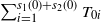 $\sum_{i=1}^{s_1(0) + s_2(0)} T_{0i}$
, where
 $T_{0i}$
are i.i.d. copies of
 $T_0$
(3.1). Since
 $\boldsymbol{{s}}(0)\ge \boldsymbol{{p}}(0)$
and
 $\boldsymbol{{s}}(0)\ge \boldsymbol{{q}}(0)$
componentwise, Lemma 2 (applied to the coupled pairs
 $(\boldsymbol{{s}},\boldsymbol{{p}})$
and
 $(\boldsymbol{{s}},\boldsymbol{{q}})$
) implies that, for all
 $t \ge 0$
,
 $\boldsymbol{{s}}(t)\ge \boldsymbol{{p}}(t)$
and
 $\boldsymbol{{s}}(t)\ge \boldsymbol{{q}}(t)$
componentwise. Thus, for any
 $t \ge 0$
,
 $\boldsymbol{{s}}(t)=(0, 0)$
implies
 $\boldsymbol{{p}}(t)=(0, 0)$
and
 $\boldsymbol{{q}}(t)=(0, 0)$
, and hence
 $T \le T'$
almost surely. Since
 $T' \preceq \sum_{i=1}^{s_1(0) + s_2(0)} T_{0i}$
, we have
 \begin{align} \mathbb{E}[T] \le \mathbb{E}[T'] & = \mathbb{E}_{\boldsymbol{{s}}(0)}[\mathbb{E}[T'] \mid \boldsymbol{{s}}(0)] \nonumber \\ & \le \mathbb{E}_{\boldsymbol{{s}}(0)}[(s_1(0)+s_2(0))\mathbb{E}[T_0]] \nonumber \\ & = \mathbb{E}_{\boldsymbol{{q}}(0)}\big[\!\max\{q_1(0),p_1(0)\} + \max\{q_2(0),p_2(0)\}\big]\mathbb{E}[T_0]. \end{align}
Using
 $\max\{x,y\} \le x+y$
for
 $x,y \ge 0$
and
 $\boldsymbol{{q}}(0) \buildrel {\mathrm{d}} \over = \pi$
, (3.5) implies that
 \begin{equation*} \mathbb{E}[T] \le \mathbb{E}[T_0]\big((x_1+x_2) + \mathbb{E}_\pi[q_1 + q_2]\big). \end{equation*}
Using
 $\mathbb{E}_\pi[q_1+ q_2] \leq {\rho(2 - \rho)}/({1-\rho})$
from Proposition 2 and recalling that
 \begin{align*}\mathbb{E}[T_0] \leq \frac{1}{\lambda}\frac{\rho(2 - \rho)}{(1-\rho)^2} = \frac{2-\rho}{2\mu(1-\rho)^2}\end{align*}
from (3.4) in Lemma 4, we obtain
 $\mathbb{E}[T] \le C_1(\lambda,\mu,\boldsymbol{{x}})$
, (2.2). Applying Markov’s inequality
 $\mathbb{P}(T \ge t) \leq {\mathbb{E}[T]}/{t}$
for
 $t > 0$
, we obtain
 $\mathbb{P}(T \ge t) \le ({1}/{t})C_1(\lambda,\mu,\boldsymbol{{x}})$
and we complete the proof of Lemma 1.
3.4. Proof of Lemma 2
Proof. Consider the processes
 $\mathcal{N}_\mathrm{a}(t)$
,
 $\mathcal{N}_\mathrm{d}^1(t)$
, and
 $\mathcal{N}_\mathrm{d}^2(t)$
in (3.2). Fix a sample path. Let
 $t_1$
be the first time that either an arrival or a potential service completion event occurs. In words,
 $t_1$
is the smallest time t such that
 $\mathcal{N}_\mathrm{a}(t)=1$
or
 $\mathcal{N}_\mathrm{d}^1(t) = 1$
or
 $\mathcal{N}_\mathrm{d}^2(t) = 1$
. We will show that
 $p_i(t_1) \ge q_i(t_1)$
.
-
(i) If the first event is a potential service completion, then as we assume the two systems are coupled, we have
 $\textrm{d}p_j(t_1) = -{1}_{\{p_j(0) \ge 1\}}$
and
$\textrm{d}q_j(t_1) = -{1}_{\{q_j(0) \ge 1\}}$
, where j is the index such that
$\mathcal{N}_\mathrm{d}^j(t_1) = 1$
. It is easy to verify that
$p_i(t_1) \ge q_i(t_1)$
for
$i \in \{1,2\}$
given
$p_i(0) \ge q_i(0)$
.
-
(ii) Next, suppose that the first event is an arrival. For contradiction, assume that
$p_j(t_1)<q_j(t_1)$
for some
$j\in\{1,2\}$
. Since
$p_j(0)\ge q_j(0)$
and only one arrival occurs at time
$t_1$
, we must have(3.6)and at time
\begin{equation} p_j(0)=q_j(0), \end{equation}
$t_1$
, the arrival must be routed to queue
$3-j$
in the p-system and to queue j in the q-system. Thus, the JSQ rule implies that
$p_{3-j}(0) \leq p_j(0)$
and
$q_j(0) \leq q_{3-j}(0)$
. Combining these inequalities with
$\boldsymbol{{p}}(0) \ge \boldsymbol{{q}}(0)$
and (3.6), we obtainEvery inequality in the above chain must therefore be an equality. Thus,
\[ p_{3-j}(0) \geq q_{3-j}(0) \geq q_j(0) = p_j(0) \geq p_{3-j}(0). \]
$p_1(0) = p_2(0)$
and
$q_1(0) = q_2(0)$
. By the deterministic tie-breaking rule, at
$t_1$
both systems must route the arrival to queue 1, contradicting the fact that the arrival is routed to queue j in one system and to queue
$3-j$
in the other.







Combining the above two cases, we show that
 $p_i(t_1) \ge q_i(t_1)$
for
 $i \in \{1,2\}$
. Proceeding in the same way, we show that
 $p_i(t) \ge q_i(t)$
for any
 $t \ge 0$
and
 $i \in \{1,2\}$
.
Next, we will show that
 $r(t) \le r(0)$
holds for every
 $t \ge 0$
. We fix a sample path. Consider the processes
 $\mathcal{N}_\mathrm{a}(t)$
,
 $\mathcal{N}_\mathrm{d}^1(t)$
, and
 $\mathcal{N}_\mathrm{d}^2(t)$
in (3.2). Let t denote the first time that either an arrival or a potential service completion event occurs.
-
(i) If the first event is an arrival, then it is obvious that
$r(t) = r(0)$
. -
(ii) If the first event is a potential service completion, then we let i denote the index such that
$\mathcal{N}_\mathrm{d}^i(t) = 1$
. Since
$\boldsymbol{{p}}(0) \ge \boldsymbol{{q}}(0)$
, we have
$p_i(t) \ge q_i(t)$
as shown above. Thus, there are two cases:-
•
${1}_{\{p_i(t-) > 0\}} = {1}_{\{q_i(t-) > 0\}}$
, which implies
$r(t) = r(0)$
. -
•
$p_i(t-) > 0$
and
$q_i(t-) = 0$
, and
$\textrm{d}p_i(t) = -1$
and
$\textrm{d}q_i(t) = 0$
, which implies that
$r(t) \le r(0)$
.
-





Combining the two cases, we show that
 $r(t) \le r(0)$
for the t defined above. Using the same argument, we show that
 $r(t) \le r(0)$
holds for every
 $t \ge 0$
.
3.5. Proof of Lemma 3
Proof. Consider two coupled JSQ systems with queue length processes
 $\boldsymbol{{p}}(t)$
and
 $\boldsymbol{{q}}(t)$
as governed by (3.2). Suppose
 $\boldsymbol{{p}}(0)=(x+1,y)$
and
 $\boldsymbol{{q}}(0)=(x,y)$
for some
 $x \ge 0$
,
 $y \ge 0$
. From Lemma 2, for any
 $t \ge 0$
,
 $\boldsymbol{{q}}(t) = (0, 0)$
implies that
 $\boldsymbol{{p}}(t) \in \{(1, 0),(0,1),(0, 0)\}$
.
Next, we show that
 $T(0,1) \buildrel \mathrm{d} \over = T(1, 0) \buildrel \mathrm{d} \over = T_0$
. We couple two copies of the JSQ system, with queue-length processes
 $\boldsymbol{{q}}^{(1)}$
and
 $\boldsymbol{{q}}^{(2)}$
, started from (1, 0) and (0,1), respectively. We use the same arrival process in both systems and couple the service-completion times of their unique initial jobs to be identical. Thus, if the service completion occurs before the first arrival, both systems move to (0, 0); if an arrival occurs first, both systems move to (1,1). Hence, under this coupling, the two copies are in the same post-jump state at the first event time. From that time onward, we couple them using the same arrival and potential service processes, so that they evolve identically. Thus,
 $T(0,1) \buildrel {\mathrm{d}} \over = T(1, 0) \buildrel {\mathrm{d}} \over = T_0$
.
Combining
 $\boldsymbol{{q}}(t) = (0, 0) \Rightarrow \boldsymbol{{p}}(t) \in \{(1, 0),(0,1),(0, 0)\}$
for all
 $t \ge 0$
,
 $T(0,1) \buildrel {\mathrm{d}} \over = T(1, 0) \buildrel {\mathrm{d}} \over = T_0$
, and the strong Markov property, we have
 $\mathcal{T}(x+1,y) \preceq \mathcal{T}(x,y) + T_0'$
, where
 $T_0'$
is an independent copy of
 $T_0$
. Similarly, we can show that
 $\mathcal{T}(x,y+1) \preceq \mathcal{T}(x,y) + T_0'$
. Iterating these one-step bounds yields
 $T(x_1,x_2) \preceq \sum_{i=1}^{x_1+x_2} T_{0i}$
.
3.6. Proof of Lemma 4
Proof. Consider two independent M/M/1 queues with arrival rates
 $\lambda/2$
and service rates
 $\mu$
, and denote their queue lengths as
 $q^{\text{M}}_1(t)$
and
 $q^{\text{M}}_2(t)$
. Then their Cartesian product,
 $\boldsymbol{{q}}^{\text{M}}(t) = (q^{\text{M}}_1(t),q^{\text{M}}_2(t))$
, is also a CTMC. Since each marginal queue is irreducible and positive recurrent under the condition
 $\lambda/2 < \mu$
, it follows that the joint process
 $\boldsymbol{{q}}^{\text{M}}(t)$
is also irreducible and positive recurrent, with the stationary distribution given by the product of the two marginal stationary distributions. Under stationarity,
 $\mathbb{P}(q^{\text{M}}_1 = k) = \mathbb{P}(q^{\text{M}}_2 = k) = \rho^k(1-\rho)$
for all
 $k \in \mathbb{Z}_+$
. Since they are independent,
 $\mathbb{P}_{\pi^{\text{M}}}\left(q^{\text{M}}_1=q^{\text{M}}_2=0\right) = (1-\rho)^2$
, where
 $\pi^{\text{M}}$
is the stationary distribution of
 $\boldsymbol{{q}}^{\text{M}}$
.
Let
 $m^{\text{M}}_{(0, 0)}$
denote the expected time for
 $\boldsymbol{{q}}^{\text{M}}$
to return to (0, 0) when starting from (0, 0), including the holding time in (0, 0). Applying [Reference Norris13, Theorem 3.5.3] to
 $\boldsymbol{{q}}^{\text{M}}$
, and noting that the total transition rate out of state (0, 0) is
 $\nu^{\text{M}}_{(0, 0)}=\lambda$
, we obtain
 \begin{equation} m^{\text{M}}_{(0, 0)} = \frac{1}{\nu^{\text{M}}_{(0, 0)} \mathbb{P}_{\pi^{\text{M}}}\left( {q^{\text{M}}_1=q^{\text{M}}_2=0}\right)} = \frac{1}{\lambda (1-\rho)^2}. \end{equation}
Starting from state (0, 0), the process
 $\boldsymbol{{q}}^{\text{M}}$
leaves (0, 0) after an
 $\mathrm{Exp}(\lambda)$
time and moves to either (1, 0) or (0,1). Let
 $T_{(1, 0)}^{(0, 0)}$
be the time for
 $\boldsymbol{{q}}^{\text{M}}$
to hit state (0, 0) starting from state (1, 0). By symmetry,
 \begin{equation*} m^{\text{M}}_{(0, 0)} = \frac{1}{\lambda} + \mathbb{E}\big[T^{(0, 0)}_{(1, 0)}\big]. \end{equation*}
Combining the above equation with (3.7), we have
 \begin{equation} \mathbb{E}\big[T^{(0, 0)}_{(1, 0)}\big] = \frac{1}{\lambda}\bigg(\frac{1}{(1-\rho)^2} - 1\bigg) = \frac{1}{\lambda}\frac{\rho (2 - \rho)}{(1-\rho)^2}. \end{equation}
Next, consider a two-queue JSQ system
 $\boldsymbol{{q}}^{\text{J}}(t)=(q^{\text{J}}_1(t),q^{\text{J}}_2(t))$
(with an arrival rate
 $\lambda$
and service rate
 $\mu$
at each queue) and the product chain
 $\boldsymbol{{q}}^{\text{M}}(t)=(q^{\text{M}}_1(t),q^{\text{M}}_2(t))$
of the two independent M/M/1 queues defined previously, both started from the same initial state
 $\boldsymbol{{q}}^{\text{J}}(0)=\boldsymbol{{q}}^{\text{M}}(0)=(1, 0)$
. By [Reference Turner18, Theorem 4], there exists a coupling of
 $\{\boldsymbol{{q}}^{\text{J}}(t)\}_{t\ge0}$
and
 $\{\boldsymbol{{q}}^{\text{M}}(t)\}_{t\ge0}$
such that
 \begin{equation} \sum_{i=1}^2 \Big[q^{\text{J}}_i(t)-x \Big]_+ \le \sum_{i=1}^2 \Big[q^{\text{M}}_i(t)-x\Big]_+ \quad \text{for all}\ x \ge 0, t \ge 0, \end{equation}
where
 $[x]_+ = \max\{x, 0\}$
. In particular, taking
 $x=0$
in (3.9) yields
 $\sum_{i=1}^2q^{\text{J}}_i(t)\le \sum_{i=1}^2 q^{\text{M}}_i(t)$
for all
 $t\ge0$
. It follows that
 \begin{align*} T_0 = \inf\{t \ge 0 \colon \boldsymbol{{q}}^{\text{J}}(t)=(0, 0)\} \le \inf\{t \ge 0 \colon \boldsymbol{{q}}^{\text{M}}(t)=(0, 0)\} = T^{(0, 0)}_{(1, 0)} \quad\text{almost surely.} \end{align*}
Using the above inequality and (3.8), we have shown that
 \begin{align*}\mathbb{E}[T_0] \le \mathbb{E}\big[T^{(0, 0)}_{(1, 0)}\big] = \frac{1}{\lambda}\frac{\rho (2 - \rho)}{(1-\rho)^2},\end{align*}
and we have completed the proof.
4. Conclusion and future work
In this paper we present a convergence rate result for a load-balancing system with two queues under the JSQ policy, which is valid for any
 $\rho \in (0,1)$
. Our method is based on a novel and simple coupling construction and on computing an upper bound on the expected hitting time. Instead of relying on approximations of the stochastic systems in relevant limits, we directly analyze the original system, yielding clean insights regarding the convergence rate and how it depends on
 $\rho$
.
We now consider some interesting future directions. Recall that we have established a convergence rate that is of order
 $O(({1}/{(1-\rho)^3})({1}/{t}))$
. However, based on the results for a single-server queue [Reference Robert14] and also based on the scaling used in diffusion approximations, we expect an exponential convergence rate of the form
 $O(\mathrm{e}^{-\alpha\varepsilon^2t})$
with
 $\varepsilon = 1- \rho$
for an appropriate constant
 $\alpha$
. Establishing such a strong bound on convergence is a future research direction, and we believe it requires adopting novel methodological approaches, particularly by exploiting state-space collapse results from the literature. Another possible approach is to compute an upper bound on the moment-generating function of the hitting time. An alternative direction is to extend our analysis to a system with
 $n \ge 3$
servers and heterogeneous service rates. We also hope the technique we have developed in this paper can spur further analysis of more complicated stochastic systems.
Acknowledgements
The authors would like to thank the editor, the editor-in-chief, and the three referees for their continued consideration and helpful feedback, which greatly improved the quality of this paper. We would also like to thank Sushil Varma and Daniela Hurtado Lange for helpful discussions during the early stages of this work.
Funding information
This work was partially supported by NSF grants EPCN-2144316 and CMMI-2140534.
Competing interests
There were no competing interests to declare which arose during the preparation or publication process of this article.

 Open access

