2.1 Partial numerical verification of GRH

In 2013, Platt provided a partial numerical verification of the GRH which asserts that all zeros of Dirichlet $L$ -functions inside the critical strip $0<\mathfrak{Re}\,s<1$ lie on the vertical $1/2$ -line.

This improves drastically both numerically and theoretically on Rumely’s work (see [Reference Ramaré and Rumely24] and [Reference Bennett2]). It increases, by a factor of $1000$ , the number of moduli for which the verification was undertaken, and it increases, by a factor of between $100$ and $10\,000$ , the size of the height $H_{q}$ (for comparable moduli). This theorem has many important applications and has already contributed to Helfgott’s proof of the ternary Goldbach conjecture [Reference Helfgott10] and [Reference Helfgott11].

2.2 Explicit zero-free regions

Theorem 2.2 [Reference McCurley19, Theorem 1].

Let $\mathfrak{L}_{q}(s)$ be the product of the $\unicode[STIX]{x1D719}(q)$ Dirichlet $L$ -functions formed with characters modulo $q$ . Let $M=\max \{q,q|\mathfrak{Im}\,s|,10\}$ and $R=9.645908801$ . Then $\mathfrak{L}_{q}(s)$ has at most a single zero in the region

$$\begin{eqnarray}\biggl\{s:\mathfrak{Re}\,s\geqslant 1-\frac{1}{R\log M}\biggr\}.\end{eqnarray}$$

The only possible zero in this region is a simple real zero arising from an $L$ -function formed with a real non-principal character modulo $q$ .

In the PhD Dissertation [Reference Kadiri13] it was established that $6.4355$ is an admissible constant for $R$ .

2.3 Explicit estimate of the number of zeros in a box

We denote $N(T,\unicode[STIX]{x1D712})$ as the number of zeros of $L(s,\unicode[STIX]{x1D712})$ in the rectangle $0<\mathfrak{Re}\,s<1$ and $|\mathfrak{Im}\,s|<T$ .

Theorem 2.3. Let $\unicode[STIX]{x1D712}$ be a primitive non-principal character modulo $q$ . Then there exist $C_{1},C_{2}>0$ s.t. for every $T\geqslant 10$

$$\begin{eqnarray}\biggl|N(T,\unicode[STIX]{x1D712})-\frac{T}{\unicode[STIX]{x1D70B}}\log \biggl(\frac{qT}{2\unicode[STIX]{x1D70B}e}\biggr)\biggr|\leqslant C_{1}\log (qT)+C_{2}.\end{eqnarray}$$

In other words,

$$\begin{eqnarray}\displaystyle N_{2}(T,q)\leqslant N(T,\unicode[STIX]{x1D712})\leqslant N_{1}(T,q) & & \displaystyle \nonumber\end{eqnarray}$$

with

$$\begin{eqnarray}\displaystyle N_{j}(T,q)=\frac{T}{\unicode[STIX]{x1D70B}}\log \frac{qT}{2\unicode[STIX]{x1D70B}e}+(-1)^{j+1}(C_{1}\log (qT)+C_{2}). & & \displaystyle \nonumber\end{eqnarray}$$

Theorem 2.3 was first established by McCurley [Reference McCurley19, Theorem 2.1]. We use here Trudgian’s version [Reference Trudgian28, Theorem 1] with

(2.1) $$\begin{eqnarray}C_{1}=0.247,\qquad C_{2}=8.949.\end{eqnarray}$$

3.1 Notation

Let $q$ be a modulus for which the verification of the GRH up to height $H_{q}$ has been established. In this article, we use Theorem 2.1 and assume that

$$\begin{eqnarray}2\leqslant q\leqslant 400\,000,\qquad H_{q}>293,\quad \text{and}\quad qH_{q}\geqslant Q_{0}=10^{8}.\end{eqnarray}$$

Let $q_{0},q_{1}$ be positive fixed integers so that $q_{0}\leqslant q\leqslant q_{1}.$ For computational purposes we split in two cases $3\leqslant q\leqslant 1000$ and $1001\leqslant q\leqslant 400\,000$ , so $q_{0}=3,q_{1}=1000,H_{q}\geqslant 100\,000$ and $q_{0}=1000,q_{1}=400\,000,H_{q}\geqslant 293$ respectively.

Let $\unicode[STIX]{x1D712}$ be a non-principal primitive character of conductor $q$ and let $\unicode[STIX]{x1D71A}_{0}=\unicode[STIX]{x1D6FD}_{0}+\text{i}\unicode[STIX]{x1D6FE}_{0}$ be a non-trivial zero of $L(s,\unicode[STIX]{x1D712})$ satisfying

(3.1) $$\begin{eqnarray}\unicode[STIX]{x1D6FE}_{0}\geqslant H_{q},\qquad q\unicode[STIX]{x1D6FE}_{0}\geqslant Q_{0},\quad \text{and}\quad \unicode[STIX]{x1D6FD}_{0}<1-\frac{1}{R\log (q|\mathfrak{Im}\,\unicode[STIX]{x1D6FE}_{0}|)}\quad \text{with }~R=9.646.\end{eqnarray}$$

We introduce the parameters $r$ and $\unicode[STIX]{x1D702}$ such that

(3.2) $$\begin{eqnarray}5\leqslant r\leqslant R\quad \text{and}\quad \unicode[STIX]{x1D702}=1-\unicode[STIX]{x1D6FD}_{0}=\frac{1}{r\log (q\unicode[STIX]{x1D6FE}_{0})}.\end{eqnarray}$$

Note that $r<5$ proves a zero-free region with admissible constant $5$ .

Let $P$ be a trigonometric polynomial of degree $n_{0}\geqslant 2$ satisfying

(3.3) $$\begin{eqnarray}P(x)=\mathop{\sum }_{k=0}^{n_{0}}a_{k}\cos (kx)\geqslant 0\quad \text{with }~a_{k}\geqslant 0,~\text{and}~0<a_{0}<a_{1}.\end{eqnarray}$$

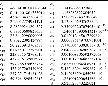
We denote $A=\sum _{k=1}^{n_{0}}a_{k}.$ We refer to §5.6 for the explicit definition of the polynomial used in this article. Here we use a polynomial of degree $n_{0}=16$ .

Let $t_{0}>0$ (here $t_{0}=100$ ) and let

(3.4) $$\begin{eqnarray}\displaystyle & \displaystyle \unicode[STIX]{x1D70E}=1-\frac{1}{R\log (q(n_{0}\unicode[STIX]{x1D6FE}_{0}+t_{0}))}, & \displaystyle\end{eqnarray}$$

(3.5) $$\begin{eqnarray}\displaystyle & \displaystyle \unicode[STIX]{x1D714}=\unicode[STIX]{x1D714}(\unicode[STIX]{x1D702},q)=\frac{1-\unicode[STIX]{x1D70E}}{\unicode[STIX]{x1D702}}=\frac{1}{R\unicode[STIX]{x1D702}\log (q(n_{0}\unicode[STIX]{x1D6FE}_{0}+t_{0}))}=\frac{1}{R\unicode[STIX]{x1D702}\log (n_{0}\text{e}^{1/r\unicode[STIX]{x1D702}}+qt_{0})}. & \displaystyle \nonumber\\ \displaystyle & & \displaystyle\end{eqnarray}$$

Since $q\unicode[STIX]{x1D6FE}_{0}\geqslant Q_{0}$ , we have the ranges

(3.6) $$\begin{eqnarray}\max (\unicode[STIX]{x1D6FD}_{0},\unicode[STIX]{x1D70E}_{0})<\unicode[STIX]{x1D70E}<1\quad \text{with }\unicode[STIX]{x1D70E}_{0}=1-\frac{1}{R\log (Q_{0}n_{0}+q_{0}t_{0})},\end{eqnarray}$$

and

(3.7) $$\begin{eqnarray}0<\unicode[STIX]{x1D702}\leqslant \unicode[STIX]{x1D702}_{0}\quad \text{with }\unicode[STIX]{x1D702}_{0}=\frac{1}{r\log Q_{0}}.\end{eqnarray}$$

Let $\unicode[STIX]{x1D702}_{1}\in (0,\unicode[STIX]{x1D702}_{0})$ . We have

(3.8) $$\begin{eqnarray}\displaystyle & & \displaystyle \left\{\begin{array}{@{}l@{}}\displaystyle \unicode[STIX]{x1D714}_{1}\leqslant \unicode[STIX]{x1D714}\leqslant \frac{r}{R}\quad \text{when }~0<\unicode[STIX]{x1D702}\leqslant \unicode[STIX]{x1D702}_{1},\quad \\ \displaystyle \unicode[STIX]{x1D714}_{0}\leqslant \unicode[STIX]{x1D714}\leqslant \unicode[STIX]{x1D714}_{1}\quad \text{when }~\unicode[STIX]{x1D702}_{1}<\unicode[STIX]{x1D702}\leqslant \unicode[STIX]{x1D702}_{0},\quad \end{array}\right.\end{eqnarray}$$

with

$$\begin{eqnarray}\displaystyle \unicode[STIX]{x1D714}_{0}=\unicode[STIX]{x1D714}(\unicode[STIX]{x1D702}_{0},q_{1})=\frac{r\log Q_{0}}{R\log (n_{0}Q_{0}+t_{0}q_{1})} & & \displaystyle \nonumber\end{eqnarray}$$

and

(3.9) $$\begin{eqnarray}\displaystyle \unicode[STIX]{x1D714}_{1}=\unicode[STIX]{x1D714}(\unicode[STIX]{x1D702}_{1},q_{0})=\frac{1}{R\unicode[STIX]{x1D702}_{1}\log (n_{0}\text{e}^{1/r\unicode[STIX]{x1D702}_{1}}+q_{0}t_{0})}. & & \displaystyle\end{eqnarray}$$

Let $\unicode[STIX]{x1D6FF},\unicode[STIX]{x1D705}$ be some parameters satisfying

(3.10) $$\begin{eqnarray}0.5<\unicode[STIX]{x1D6FF}<0.75,\quad \text{and}\quad 0.25<\unicode[STIX]{x1D705}<\min \biggl(\frac{\unicode[STIX]{x1D70E}_{0}}{1+\unicode[STIX]{x1D6FF}},\frac{1}{2\unicode[STIX]{x1D6FF}+1}\biggr).\end{eqnarray}$$

In addition, we assume

(3.11) $$\begin{eqnarray}\max (10,((\unicode[STIX]{x1D705}(2\unicode[STIX]{x1D6FF}+1))^{-1}-1)^{-1/2})<t_{0}<293<H_{q}.\end{eqnarray}$$

We provide in Proposition 5.2 the definitions of $\unicode[STIX]{x1D705}$ and $\unicode[STIX]{x1D6FF}$ depending on $h$ , $\unicode[STIX]{x1D70E}_{0}$ , and  $\unicode[STIX]{x1D702}_{0}$ .

Finally, we add the condition

(3.12) $$\begin{eqnarray}a_{0}+\biggl(\frac{1-\unicode[STIX]{x1D705}}{\max (\frac{1}{2^{\unicode[STIX]{x1D70E}_{0}}-1}-\frac{\unicode[STIX]{x1D705}}{2^{\unicode[STIX]{x1D70E}_{0}+\unicode[STIX]{x1D6FF}}-1},2(\frac{1}{3^{\unicode[STIX]{x1D70E}_{0}}-1}-\frac{\unicode[STIX]{x1D705}}{3^{\unicode[STIX]{x1D70E}_{0}+\unicode[STIX]{x1D6FF}}-1}))}-1\biggr)\mathop{\sum }_{k=2}^{n_{0}}a_{k}>0.\end{eqnarray}$$

Numerical data for all the above parameters ( $r,\unicode[STIX]{x1D705},\unicode[STIX]{x1D6FF}$ ) are given in Tables 2 and 3, §5.7.

3.2 Introducing a smooth weight

We now introduce the weight $f$ which is used in the study of $\sum _{n\geqslant 1}(\unicode[STIX]{x1D712}(n)\unicode[STIX]{x1D6EC}(n)/n^{s})f(\log n)(1-\unicode[STIX]{x1D705}/n^{\unicode[STIX]{x1D6FF}})$ . We define

(3.13) $$\begin{eqnarray}f(t)=f_{\unicode[STIX]{x1D702}}(t)=\unicode[STIX]{x1D702}h(\unicode[STIX]{x1D702}t),\end{eqnarray}$$

where $h$ is a function satisfying

(3.14) $$\begin{eqnarray}\left\{\begin{array}{@{}l@{}}h\text{ is compactly supported in }[0,d]\quad \text{for some }~d>0,\quad \\ h\text{ is positive in }[0,d),\quad \\ h\in {\mathcal{C}}^{2}([0,d]),\quad \\ h(d)=h^{\prime }(0)=h^{\prime }(d)=h^{\prime \prime }(d)=0.\quad \end{array}\right.\end{eqnarray}$$

Note that in [Reference Kadiri14], we used the notation $g_{1}(\unicode[STIX]{x1D703})$ and $m$ instead of $h(0)$ and $m_{h}$ respectively. We give more details in §5.5 on the motivation for the explicit choice for $f$ as well as study its analytical properties.

We denote $F$ the Laplace transform of $f$ :

(3.15) $$\begin{eqnarray}F(s)=\int _{0}^{\infty }\text{e}^{-st}f(t)\,dt=\int _{0}^{d}\text{e}^{-su/\unicode[STIX]{x1D702}}h(u)\,du,\end{eqnarray}$$

$F_{2}$ the Laplace transform of $f^{\prime \prime }$ , and

(3.16) $$\begin{eqnarray}H(x,y)=\mathfrak{Re}\biggl(\frac{F_{2}(x+\text{i}y)}{(x+\text{i}y)^{2}}\biggr).\end{eqnarray}$$

We impose a last and important condition on $f$ : that its Laplace transform satisfies

(3.17) $$\begin{eqnarray}\mathfrak{Re}\,F(z)\geqslant 0\quad \text{when }~\mathfrak{Re}\,z\geqslant 0.\end{eqnarray}$$

We now recall some properties established in [Reference Kadiri14, Lemma 3.2].

Lemma 3.1. Let $x,y$ be real numbers satisfying $x+\text{i}y\not =0$ .

(3.18) $$\begin{eqnarray}\mathfrak{Re}\,F(x+\text{i}y)=\frac{x}{x^{2}+y^{2}}h(0)\unicode[STIX]{x1D702}+H(x,y),\end{eqnarray}$$

where

(3.19) $$\begin{eqnarray}~|H(x,y)|\leqslant \frac{M(x/\unicode[STIX]{x1D702})}{x^{2}+y^{2}}\unicode[STIX]{x1D702}^{2}\quad \text{with }M(z)=\int _{0}^{d}|h^{\prime \prime }(u)|\text{e}^{-zu}\,du.\quad\end{eqnarray}$$

In addition, when $x\geqslant 0$ , then

(3.20) $$\begin{eqnarray}|H(x,y)|\leqslant \frac{m_{h}}{x(x^{2}+y^{2})}\unicode[STIX]{x1D702}^{3}\quad \text{with }m_{h}=\max _{u\in [0,d]}|h^{\prime \prime }(u)|.\end{eqnarray}$$

3.3 An explicit formula for a smoothed version of $-(L^{\prime }/L)(s,\unicode[STIX]{x1D712})$

Proposition 3.2. Let $f$ be a function satisfying (3.14). Let $s$ be a complex number, and $\unicode[STIX]{x1D712}$ a primitive (non-principal) character modulo $q$ . Then

(3.21) $$\begin{eqnarray}\displaystyle & & \displaystyle \mathfrak{Re}\mathop{\sum }_{n\geqslant 1}\frac{\unicode[STIX]{x1D6EC}(n)\unicode[STIX]{x1D712}(n)f(\log n)}{n^{s}}\nonumber\\ \displaystyle & & \displaystyle \qquad =-\mathfrak{Re}\mathop{\sum }_{\unicode[STIX]{x1D71A}\in Z(\unicode[STIX]{x1D712})}F(s-\unicode[STIX]{x1D71A})+\frac{f(0)}{2}\biggl(\log \frac{q}{\unicode[STIX]{x1D70B}}+\mathfrak{Re}\,\frac{\unicode[STIX]{x1D6E4}^{\prime }}{\unicode[STIX]{x1D6E4}}\biggl(\frac{s+\mathfrak{a}}{2}\biggr)\biggr)\nonumber\\ \displaystyle & & \displaystyle \qquad \quad +\,\mathfrak{Re}\,\frac{1}{2\text{i}\unicode[STIX]{x1D70B}}\int _{1/2-\text{i}\infty }^{1/2+\text{i}\infty }\mathfrak{Re}\,\frac{\unicode[STIX]{x1D6E4}^{\prime }}{\unicode[STIX]{x1D6E4}}\biggl(\frac{z+\mathfrak{a}}{2}\biggr)\frac{F_{2}(s-z)}{(s-z)^{2}}\,dz,\end{eqnarray}$$

(3.22) $$\begin{eqnarray}\displaystyle & & \displaystyle \mathfrak{Re}\mathop{\sum }_{n\geqslant 1}\frac{\unicode[STIX]{x1D6EC}(n)f(\log n)}{n^{s}}\nonumber\\ \displaystyle & & \displaystyle \qquad \!\!=\mathfrak{Re}\,F(s-1)-\!\mathop{\sum }_{\unicode[STIX]{x1D71A}\in Z(\unicode[STIX]{x1D701})}\!\mathfrak{Re}\,F(s-\unicode[STIX]{x1D71A})+\frac{f(0)}{2}\biggl(-\log \,\unicode[STIX]{x1D70B}+\mathfrak{Re}\,\frac{\unicode[STIX]{x1D6E4}^{\prime }}{\unicode[STIX]{x1D6E4}}\biggl(\frac{s}{2}+1\biggr)\biggr)\nonumber\\ \displaystyle & & \displaystyle \qquad \quad +\,\mathfrak{Re}\,\frac{F_{2}(s)}{s^{2}}+\mathfrak{Re}\,\frac{1}{2\text{i}\unicode[STIX]{x1D70B}}\int _{1/2-\text{i}\infty }^{1/2+\text{i}\infty }\mathfrak{Re}\,\frac{\unicode[STIX]{x1D6E4}^{\prime }}{\unicode[STIX]{x1D6E4}}\biggl(\frac{z}{2}\biggr)\frac{F_{2}(s-z)}{(s-z)^{2}}\,dz,\end{eqnarray}$$

where $Z(\unicode[STIX]{x1D701})$ and $Z(\unicode[STIX]{x1D712})$ are the sets of non-trivial zeros of $\unicode[STIX]{x1D701}(s)$ and of $L(s,\unicode[STIX]{x1D712})$ , respectively.

Proof of Proposition 3.2 is postponed until §6.2. The case of the principal character $\unicode[STIX]{x1D712}_{0}$ follows from (3.22) and the identity

$$\begin{eqnarray}\displaystyle \mathfrak{Re}\mathop{\sum }_{n\geqslant 1}\frac{\unicode[STIX]{x1D6EC}(n)\unicode[STIX]{x1D712}_{0}(n)f(\log n)}{n^{s}} & = & \displaystyle \mathfrak{Re}\mathop{\sum }_{n\geqslant 1}\frac{\unicode[STIX]{x1D6EC}(n)f(\log n)}{n^{s}}\nonumber\\ \displaystyle & & \displaystyle -\,\mathfrak{Re}\mathop{\sum }_{m\geqslant 1}\mathop{\sum }_{p\mid q}\frac{(\log p)f(m\log p)}{p^{ms}}.\nonumber\end{eqnarray}$$

Let $s=x+\text{i}y$ be a complex number. For $\unicode[STIX]{x1D705},\unicode[STIX]{x1D6FF}$ as defined in (3.10), we introduce

(3.23) $$\begin{eqnarray}\displaystyle & \displaystyle S(s)=\mathfrak{Re}\mathop{\sum }_{n\geqslant 1}\frac{\unicode[STIX]{x1D6EC}(n)f(\log n)}{n^{s}}\biggl(1-\frac{\unicode[STIX]{x1D705}}{n^{\unicode[STIX]{x1D6FF}}}\biggr), & \displaystyle\end{eqnarray}$$

(3.24) $$\begin{eqnarray}\displaystyle & \displaystyle S(s,\unicode[STIX]{x1D712})=\mathfrak{Re}\mathop{\sum }_{n\geqslant 1}\frac{\unicode[STIX]{x1D712}(n)\unicode[STIX]{x1D6EC}(n)f(\log n)}{n^{s}}\biggl(1-\frac{\unicode[STIX]{x1D705}}{n^{\unicode[STIX]{x1D6FF}}}\biggr). & \displaystyle\end{eqnarray}$$

(3.25) $$\begin{eqnarray}\displaystyle & \displaystyle E(x,y)=H(x,y)-\unicode[STIX]{x1D705}H(x+\unicode[STIX]{x1D6FF},y). & \displaystyle\end{eqnarray}$$

(3.26) $$\begin{eqnarray}\displaystyle D(s) & = & \displaystyle \mathfrak{Re}(F(s)-\unicode[STIX]{x1D705}F(s+\unicode[STIX]{x1D6FF}))\nonumber\\ \displaystyle & = & \displaystyle \biggl(\frac{x}{x^{2}+y^{2}}-\frac{\unicode[STIX]{x1D705}(x+\unicode[STIX]{x1D6FF})}{(x+\unicode[STIX]{x1D6FF})^{2}+y^{2}}\biggr)h(0)\unicode[STIX]{x1D702}+E(x,y),\end{eqnarray}$$

(3.27) $$\begin{eqnarray}\mathfrak{G}_{\unicode[STIX]{x1D705},\unicode[STIX]{x1D6FF}}(s)=\mathfrak{Re}\,\frac{\unicode[STIX]{x1D6E4}^{\prime }}{\unicode[STIX]{x1D6E4}}(s/2)-\unicode[STIX]{x1D705}\,\mathfrak{Re}\,\frac{\unicode[STIX]{x1D6E4}^{\prime }}{\unicode[STIX]{x1D6E4}}((s+\unicode[STIX]{x1D6FF})/2).\end{eqnarray}$$

In addition we define

(3.28) $$\begin{eqnarray}\displaystyle & \displaystyle D_{1}(s)=\frac{h(0)\unicode[STIX]{x1D702}}{2}[-(1-\unicode[STIX]{x1D705})\log \unicode[STIX]{x1D70B}+\mathfrak{G}_{\unicode[STIX]{x1D705},\unicode[STIX]{x1D6FF}}(s+2)], & \displaystyle\end{eqnarray}$$

(3.29) $$\begin{eqnarray}\displaystyle & \displaystyle D_{1}(s,\unicode[STIX]{x1D712})=\frac{h(0)\unicode[STIX]{x1D702}}{2}\biggl[(1-\unicode[STIX]{x1D705})\log \frac{q}{\unicode[STIX]{x1D70B}}+\mathfrak{G}_{\unicode[STIX]{x1D705},\unicode[STIX]{x1D6FF}}(s+\mathfrak{a})\biggr], & \displaystyle\end{eqnarray}$$

(3.30) $$\begin{eqnarray}\displaystyle & \!\displaystyle D_{2}(s)=E(x,y)+\frac{1}{2\unicode[STIX]{x1D70B}}\!\int _{-\infty }^{+\infty }\mathfrak{Re}\,\frac{\unicode[STIX]{x1D6E4}^{\prime }}{\unicode[STIX]{x1D6E4}}((1/2+\text{i}t)/2)E(x-1/2,y-t)\,dt,\qquad \ & \displaystyle\end{eqnarray}$$

(3.31) $$\begin{eqnarray}\displaystyle & \displaystyle D_{2}(s,\unicode[STIX]{x1D712})=\frac{1}{2\unicode[STIX]{x1D70B}}\!\int _{-\infty }^{+\infty }\mathfrak{Re}\,\frac{\unicode[STIX]{x1D6E4}^{\prime }}{\unicode[STIX]{x1D6E4}}((1/2+\mathfrak{a}+\text{i}t)/2)E(x-1/2,y-t)\,dt.\qquad & \displaystyle\end{eqnarray}$$

Using this notation and noting that $f(0)=h(0)\unicode[STIX]{x1D702}$ and $\mathfrak{Re}(\unicode[STIX]{x1D6E4}^{\prime }/\unicode[STIX]{x1D6E4})(s)=\mathfrak{Re}(\unicode[STIX]{x1D6E4}^{\prime }/\unicode[STIX]{x1D6E4})(s/2)$ , the explicit formulae from Proposition 3.2 become

(3.32) $$\begin{eqnarray}\displaystyle & \displaystyle S(s)=D(s-1)-\mathop{\sum }_{\unicode[STIX]{x1D71A}\in Z(\unicode[STIX]{x1D701})}D(s-\unicode[STIX]{x1D71A})+D_{1}(s)+D_{2}(s), & \displaystyle\end{eqnarray}$$

(3.33) $$\begin{eqnarray}\displaystyle & \displaystyle S(s,\unicode[STIX]{x1D712})=-\mathop{\sum }_{\unicode[STIX]{x1D71A}\in Z(\unicode[STIX]{x1D712})}D(s-\unicode[STIX]{x1D71A})+D_{1}(s,\unicode[STIX]{x1D712})+D_{2}(s,\unicode[STIX]{x1D712}). & \displaystyle\end{eqnarray}$$

3.4 An explicit inequality

Taking $x=\arg (\unicode[STIX]{x1D712}(n)/n^{\text{i}\unicode[STIX]{x1D6FE}_{0}})$ in the non-negative trigonometric inequality (3.3), we get

(3.34) $$\begin{eqnarray}\mathop{\sum }_{k=0}^{n_{0}}a_{k}S(\unicode[STIX]{x1D70E}+\text{i}k\unicode[STIX]{x1D6FE}_{0},\unicode[STIX]{x1D712}^{k})\geqslant 0.\end{eqnarray}$$

Note that Proposition 3.2 can be applied to $\unicode[STIX]{x1D712}^{k}$ only when it is a non-primitive character. So for each $k\geqslant 2$ , we introduce $q_{k}$ the conductor for the Dirichlet character $\unicode[STIX]{x1D712}^{k}$ , and $\unicode[STIX]{x1D712}_{(k)}$ the unique primitive character modulo $q_{k}$ that induces $\unicode[STIX]{x1D712}^{k}$ . (We refer the reader to [Reference Montgomery and Vaughan20, Theorem 9.2] and recall that for $k=0$ , $\unicode[STIX]{x1D712}_{(0)}$ is identically $1$ , and for $k=1,\unicode[STIX]{x1D712}_{(1)}=\unicode[STIX]{x1D712}$ .) We establish in Lemma 6.2 that under condition (3.12), then

(3.35) $$\begin{eqnarray}\mathop{\sum }_{k=0}^{n_{0}}a_{k}S(\unicode[STIX]{x1D70E}+\text{i}k\unicode[STIX]{x1D6FE}_{0},\unicode[STIX]{x1D712}_{(k)}-\unicode[STIX]{x1D712}^{k})+\frac{1-\unicode[STIX]{x1D705}}{2}f(0)\mathop{\sum }_{k=1}^{n_{0}}a_{k}\log \biggl(\frac{q}{q_{k}}\biggr)\geqslant 0.\end{eqnarray}$$

Together with (3.34) and (3.35), we obtain

(3.36) $$\begin{eqnarray}\mathop{\sum }_{k=0}^{n_{0}}a_{k}S(\unicode[STIX]{x1D70E}+\text{i}k\unicode[STIX]{x1D6FE}_{0},\unicode[STIX]{x1D712}_{(k)})+\frac{1-\unicode[STIX]{x1D705}}{2}f(0)\mathop{\sum }_{k=2}^{n_{0}}a_{k}\log \biggl(\frac{q}{q_{k}}\biggr)\geqslant 0,\end{eqnarray}$$

and we can now apply the explicit formulae from Proposition 3.2 to each “primitive term” $S(\unicode[STIX]{x1D70E}+\text{i}k\unicode[STIX]{x1D6FE}_{0},\unicode[STIX]{x1D712}_{(k)})$ . We introduce the notation

(3.37) $$\begin{eqnarray}\displaystyle {\mathcal{E}}_{1} & = & \displaystyle a_{0}D(\unicode[STIX]{x1D70E}-1)=a_{0}(F(\unicode[STIX]{x1D70E}-1,0)-\unicode[STIX]{x1D705}F(\unicode[STIX]{x1D70E}-1+\unicode[STIX]{x1D6FF},0)),\end{eqnarray}$$

(3.38) $$\begin{eqnarray}\displaystyle {\mathcal{E}}_{2} & = & \displaystyle \mathop{\sum }_{k=0}^{4}a_{k}\mathop{\sum }_{\unicode[STIX]{x1D71A}\in Z(\unicode[STIX]{x1D712}_{(k)})}D(\unicode[STIX]{x1D70E}+\text{i}k\unicode[STIX]{x1D6FE}_{0}-\unicode[STIX]{x1D71A}),\end{eqnarray}$$

(3.39) $$\begin{eqnarray}\displaystyle {\mathcal{E}}_{3} & = & \displaystyle a_{0}D_{1}(\unicode[STIX]{x1D70E})+\mathop{\sum }_{k=1}^{n_{0}}a_{k}\biggl(D_{1}(\unicode[STIX]{x1D70E}+\text{i}k\unicode[STIX]{x1D6FE}_{0},\unicode[STIX]{x1D712}_{(k)})+\frac{1-\unicode[STIX]{x1D705}}{2}f(0)\log (q/q_{k})\biggr)\nonumber\\ \displaystyle & = & \displaystyle \frac{h(0)\unicode[STIX]{x1D702}}{2} [a_{0}(-(1-\unicode[STIX]{x1D705})\log \unicode[STIX]{x1D70B}+\mathfrak{G}_{\unicode[STIX]{x1D705},\unicode[STIX]{x1D6FF}}(\unicode[STIX]{x1D70E}+2))+(1-\unicode[STIX]{x1D705})A\log (q/\unicode[STIX]{x1D70B})\nonumber\\ \displaystyle & & \displaystyle +\,\mathop{\sum }_{k=1}^{n_{0}}a_{k}\mathfrak{G}_{\unicode[STIX]{x1D705},\unicode[STIX]{x1D6FF}}(\unicode[STIX]{x1D70E}+\mathfrak{a}_{k}+\text{i}k\unicode[STIX]{x1D6FE}_{0})],\end{eqnarray}$$

(3.40) $$\begin{eqnarray}\displaystyle {\mathcal{E}}_{4} & = & \displaystyle a_{0}D_{2}(\unicode[STIX]{x1D70E})+\mathop{\sum }_{k=1}^{n_{0}}a_{k}D_{2}(\unicode[STIX]{x1D70E}+\text{i}k\unicode[STIX]{x1D6FE}_{0},\unicode[STIX]{x1D712}_{(k)})\nonumber\\ \displaystyle & = & \displaystyle a_{0}E(\unicode[STIX]{x1D70E},0)+\mathop{\sum }_{k=0}^{n_{0}}\frac{a_{k}}{2\unicode[STIX]{x1D70B}}\int _{-\infty }^{+\infty }\mathfrak{Re}\,\frac{\unicode[STIX]{x1D6E4}^{\prime }}{\unicode[STIX]{x1D6E4}}\biggl(\frac{1/2+\mathfrak{a}_{k}+\text{i}t}{2}\biggr)\nonumber\\ \displaystyle & & \displaystyle \times \,E(\unicode[STIX]{x1D70E}-1/2,k\unicode[STIX]{x1D6FE}_{0}-t)\,dt,\end{eqnarray}$$

where $\mathfrak{a}_{k}$ is associated to the character $\unicode[STIX]{x1D712}_{k}$ :

(3.41) $$\begin{eqnarray}\mathfrak{a}_{k}=\frac{1-\unicode[STIX]{x1D712}_{k}(-1)}{2}.\end{eqnarray}$$

In particular, $\mathfrak{a}_{0}=0$ . Using this notation to rewrite explicit formulae (3.32) and (3.33) respectively, we rewrite (3.36) more simply as

(3.42) $$\begin{eqnarray}0\leqslant {\mathcal{E}}_{1}-{\mathcal{E}}_{2}+{\mathcal{E}}_{3}+{\mathcal{E}}_{4}.\end{eqnarray}$$

4.1 Studying each ${\mathcal{E}}_{i}$

We make use of Lemma 3.1 for this and refer the reader to the next section for full details.

• ∙ For ${\mathcal{E}}_{1}$ , the pole of the Riemann zeta function at $s=1$ gives the contribution $a_{0}D(\unicode[STIX]{x1D70E}-1)=a_{0}F(\unicode[STIX]{x1D70E}-1)+{\mathcal{O}}(\unicode[STIX]{x1D702})=a_{0}/(\unicode[STIX]{x1D70E}-1)+{\mathcal{O}}(\unicode[STIX]{x1D702})$ . We prove in Lemma 5.1 that

  $$\begin{eqnarray}{\mathcal{E}}_{1}\leqslant a_{0}F(\unicode[STIX]{x1D70E}-1)+{\mathcal{C}}_{1}(\unicode[STIX]{x1D702}).\end{eqnarray}$$

• ∙ In the sum over the zeros ${\mathcal{E}}_{2}$ , we isolate the term at $k=1,\unicode[STIX]{x1D71A}=\unicode[STIX]{x1D6FD}_{0}+\text{i}\unicode[STIX]{x1D6FE}_{0}$ :

  $$\begin{eqnarray}a_{1}(F(\unicode[STIX]{x1D70E}-\unicode[STIX]{x1D6FD}_{0})-\unicode[STIX]{x1D705}F(\unicode[STIX]{x1D70E}+\unicode[STIX]{x1D6FF}-\unicode[STIX]{x1D6FD}_{0}))=a_{1}F(\unicode[STIX]{x1D70E}-\unicode[STIX]{x1D6FD}_{0})+{\mathcal{O}}(\unicode[STIX]{x1D702}).\end{eqnarray}$$
  The positivity property (3.17) for the Laplace transform $F$ allows us to discard most of the zeros on the right of the vertical line at $\unicode[STIX]{x1D70E}$ . This is done by means of a generalization of Stechkin’s lemma (see §5.2.2 and in particular Proposition 5.2): for $d$ the solution of the equation
  (4.1) $$\begin{eqnarray}\displaystyle & & \displaystyle (2t+1)h(0)+\biggl(\frac{1}{t}+\frac{1}{2\unicode[STIX]{x1D70E}_{0}-1+t}\biggr)m_{h}\unicode[STIX]{x1D702}_{0}^{2}\nonumber\\ \displaystyle & & \displaystyle \quad =\biggl(\frac{1}{t}+\frac{1+t}{(2\unicode[STIX]{x1D70E}_{0}-1+t)^{2}}\biggr)h(0)+\biggl(\frac{1}{t^{3}}+\frac{1}{(2\unicode[STIX]{x1D70E}_{0}-1+t)^{3}}\biggr)m_{h}\unicode[STIX]{x1D702}_{0}^{2}\nonumber\\ \displaystyle & & \displaystyle\end{eqnarray}$$
  and for
  (4.2) $$\begin{eqnarray}\unicode[STIX]{x1D705}=\frac{(2\unicode[STIX]{x1D70E}_{0}-1)h(0)-m_{h}\unicode[STIX]{x1D702}_{0}^{2}/(2\unicode[STIX]{x1D70E}_{0}-1)}{(2\unicode[STIX]{x1D6FF}+1)h(0)+(1/\unicode[STIX]{x1D6FF}+1/(2\unicode[STIX]{x1D70E}_{0}-1+\unicode[STIX]{x1D6FF}))m_{h}\unicode[STIX]{x1D702}_{0}^{2}},\end{eqnarray}$$
  then
  $$\begin{eqnarray}D(\unicode[STIX]{x1D70E}-\unicode[STIX]{x1D6FD}+\text{i}y)+D(\unicode[STIX]{x1D70E}-1+\unicode[STIX]{x1D6FD}+\text{i}y)\geqslant 0\end{eqnarray}$$
  as soon as $1/2<\unicode[STIX]{x1D6FD}<\unicode[STIX]{x1D70E}$ and $y>0$ . Finally, we use an explicit zero density estimate to prove that the remaining sum contributes negligibly. We prove in Lemma 5.4 that
  (4.3) $$\begin{eqnarray}{\mathcal{E}}_{2}\geqslant a_{1}F(\unicode[STIX]{x1D70E}-\unicode[STIX]{x1D6FD}_{0},0)+{\mathcal{C}}_{2}(\unicode[STIX]{x1D702}).\end{eqnarray}$$

• ∙ We use Stirling’s formula to estimate the Gamma terms appearing in ${\mathcal{E}}_{3}$ and ${\mathcal{E}}_{4}$ . Since $\unicode[STIX]{x1D6FE}_{0}>1$ , we have $|\mathfrak{G}_{\unicode[STIX]{x1D705},\unicode[STIX]{x1D6FF}}(\unicode[STIX]{x1D70E}+\mathfrak{a}_{k}+\text{i}k\unicode[STIX]{x1D6FE}_{0})|\leqslant \log \unicode[STIX]{x1D6FE}_{0}+{\mathcal{O}}(1)$ , for all $k\geqslant 1$ . We prove in Lemma 5.5 that

  $$\begin{eqnarray}{\mathcal{E}}_{3}\leqslant \frac{A(1-\unicode[STIX]{x1D705})h(0)}{2}\log (q\unicode[STIX]{x1D6FE}_{0})\unicode[STIX]{x1D702}+{\mathcal{C}}_{3}(\unicode[STIX]{x1D702}).\end{eqnarray}$$

• ∙ Finally, the integral term is negligible and we prove in Lemma 5.8 that

  $$\begin{eqnarray}{\mathcal{E}}_{4}\leqslant {\mathcal{C}}_{4}(\unicode[STIX]{x1D702}).\end{eqnarray}$$

The positivity argument (3.42) can then be rewritten as

(4.4) $$\begin{eqnarray}0\leqslant a_{0}F(\unicode[STIX]{x1D70E}-1)-a_{1}F(\unicode[STIX]{x1D70E}-\unicode[STIX]{x1D6FD}_{0})+\frac{A(1-\unicode[STIX]{x1D705})h(0)}{2}\log (q\unicode[STIX]{x1D6FE}_{0})\unicode[STIX]{x1D702}+\mathfrak{e}(\unicode[STIX]{x1D702}),\end{eqnarray}$$

where the error term is

(4.5) $$\begin{eqnarray}\mathfrak{e}(\unicode[STIX]{x1D702})={\mathcal{C}}_{1}(\unicode[STIX]{x1D702})+{\mathcal{C}}_{2}(\unicode[STIX]{x1D702})+{\mathcal{C}}_{3}(\unicode[STIX]{x1D702})+{\mathcal{C}}_{4}(\unicode[STIX]{x1D702}).\end{eqnarray}$$

We introduce the difference

(4.6) $$\begin{eqnarray}K_{h}(\unicode[STIX]{x1D714})=a_{1}F(\unicode[STIX]{x1D70E}-\unicode[STIX]{x1D6FD}_{0})-a_{0}F(\unicode[STIX]{x1D70E}-1)=\int _{0}^{d}(a_{1}\text{e}^{-t}-a_{0})h(t)\text{e}^{\unicode[STIX]{x1D714}t}\,dt,\end{eqnarray}$$

so that inequality (4.4) becomes

(4.7) $$\begin{eqnarray}r=\frac{1}{\log (q\unicode[STIX]{x1D6FE}_{0})\unicode[STIX]{x1D702}}\leqslant \frac{A(1-\unicode[STIX]{x1D705})h(0)}{2(K_{h}(\unicode[STIX]{x1D714})-\mathfrak{e}(\unicode[STIX]{x1D702}))}.\end{eqnarray}$$

4.2 A strategy to compute the constant in the zero-free-region

It remains to find a lower bound as large as possible for $K_{h}(\unicode[STIX]{x1D714})-\mathfrak{e}(\unicode[STIX]{x1D702})$ for the values of $\unicode[STIX]{x1D702}$ in $(0,\unicode[STIX]{x1D702}_{0})$ .

Since $(\unicode[STIX]{x2202}K_{h}/\unicode[STIX]{x2202}\unicode[STIX]{x1D714})(\unicode[STIX]{x1D714})=\int _{0}^{d}(a_{1}\text{e}^{-t}-a_{0})h(t)t\text{e}^{\unicode[STIX]{x1D714}t}\,dt,$ with $a_{1}\text{e}^{-t}-a_{0}>0$ when $t<\log (a_{1}/a_{0})$ and $\unicode[STIX]{x1D714}_{0}\leqslant \unicode[STIX]{x1D714}\leqslant r/R$ , then

$$\begin{eqnarray}\displaystyle \frac{\unicode[STIX]{x2202}K_{h}}{\unicode[STIX]{x2202}\unicode[STIX]{x1D714}}(\unicode[STIX]{x1D714}) & {>} & \displaystyle \int _{0}^{\log (a_{1}/a_{0})}(a_{1}\text{e}^{-t}-a_{0})h(t)t\text{e}^{\unicode[STIX]{x1D714}_{0}t}\,dt\nonumber\\ \displaystyle & & \displaystyle +\,\int _{\log (a_{1}/a_{0})}^{d}(a_{1}\text{e}^{-t}-a_{0})h(t)t\text{e}^{(r/R)t}\,dt.\nonumber\end{eqnarray}$$

We choose values for $\unicode[STIX]{x1D714}_{0}$ so that

(4.8) $$\begin{eqnarray}\int _{0}^{\log (a_{1}/a_{0})}(a_{1}\text{e}^{-t}-a_{0})h(t)t\text{e}^{\unicode[STIX]{x1D714}_{0}t}\,dt+\int _{ log(a_{1}/a_{0})}^{d}(a_{1}\text{e}^{-t}-a_{0})h(t)t\text{e}^{(r/R)t}\,dt>0\end{eqnarray}$$

and $K_{h}(\unicode[STIX]{x1D714})$ increases with $\unicode[STIX]{x1D714}\in (\unicode[STIX]{x1D714}_{0},r/R)$ .

From the definitions of the ${\mathcal{C}}_{i}$ in (5.2), (5.23), (5.25), and (5.40), we have

(4.9) $$\begin{eqnarray}\mathfrak{e}(\unicode[STIX]{x1D702})=\unicode[STIX]{x1D702}(\unicode[STIX]{x1D6FC}_{1}+\unicode[STIX]{x1D6FC}_{2}\unicode[STIX]{x1D702}+\unicode[STIX]{x1D6FC}_{3}\unicode[STIX]{x1D702}^{2}),\end{eqnarray}$$

where the $\unicode[STIX]{x1D6FC}_{i}$ are computable constants and satisfy $\unicode[STIX]{x1D6FC}_{1}<0,\unicode[STIX]{x1D6FC}_{2}>0$ , $\unicode[STIX]{x1D6FC}_{3}>0$ . We have that $\mathfrak{e}(\unicode[STIX]{x1D702})$ is negative and decreases from $\unicode[STIX]{x1D702}=0$ to , then it increases (becoming positive after the root ).

We are now able to establish a lower bound for $K_{h}(\unicode[STIX]{x1D714})-\mathfrak{e}(\unicode[STIX]{x1D702})$ . We fix $\unicode[STIX]{x1D702}_{1}\in (0,\unicode[STIX]{x1D702}_{0})$ and bound $K_{h}(\unicode[STIX]{x1D714})-\mathfrak{e}(\unicode[STIX]{x1D702})$ in each of the following cases, depending on the location of $\unicode[STIX]{x1D702}_{1}$ with respect to $\unicode[STIX]{x1D702}_{2}$ . We denote

(4.10) $$\begin{eqnarray}\unicode[STIX]{x1D714}_{1}=\unicode[STIX]{x1D714}(\unicode[STIX]{x1D702}_{1},q_{0}),\qquad \unicode[STIX]{x1D714}_{2}=\unicode[STIX]{x1D714}(\unicode[STIX]{x1D702}_{2},q_{0}).\end{eqnarray}$$

1. (1) If $0<\unicode[STIX]{x1D702}_{0}<\unicode[STIX]{x1D702}_{2}$ , then

   $$\begin{eqnarray}K_{h}(\unicode[STIX]{x1D714})-\mathfrak{e}(\unicode[STIX]{x1D702})>\left\{\begin{array}{@{}ll@{}}K_{h}(\unicode[STIX]{x1D714}_{1})\quad & \text{ if }~0<\unicode[STIX]{x1D702}<\unicode[STIX]{x1D702}_{1},\\ K_{h}(\unicode[STIX]{x1D714}_{0})-\mathfrak{e}(\unicode[STIX]{x1D702}_{1})\quad & \text{ if }~\unicode[STIX]{x1D702}_{1}<\unicode[STIX]{x1D702}<\unicode[STIX]{x1D702}_{0}.\end{array}\right.\end{eqnarray}$$

2. (2) If $0<\unicode[STIX]{x1D702}_{2}<\unicode[STIX]{x1D702}_{0}$ and $0<\unicode[STIX]{x1D702}_{1}<\unicode[STIX]{x1D702}_{2}$ then

   $$\begin{eqnarray}K_{h}(\unicode[STIX]{x1D714})-\mathfrak{e}(\unicode[STIX]{x1D702})>\left\{\begin{array}{@{}ll@{}}K_{h}(\unicode[STIX]{x1D714}_{1})\quad & \text{ if }~0<\unicode[STIX]{x1D702}<\unicode[STIX]{x1D702}_{1},\\ K_{h}(\unicode[STIX]{x1D714}_{0})-\max (\mathfrak{e}(\unicode[STIX]{x1D702}_{1}),\mathfrak{e}(\unicode[STIX]{x1D702}_{0}))\quad & \text{ if }~\unicode[STIX]{x1D702}_{1}<\unicode[STIX]{x1D702}<\unicode[STIX]{x1D702}_{0}.\end{array}\right.\end{eqnarray}$$

3. (3) If $0<\unicode[STIX]{x1D702}_{2}<\unicode[STIX]{x1D702}_{0}$ and $\unicode[STIX]{x1D702}_{2}<\unicode[STIX]{x1D702}_{1}<\unicode[STIX]{x1D702}_{0}$ then

   $$\begin{eqnarray}K_{h}(\unicode[STIX]{x1D714})-\mathfrak{e}(\unicode[STIX]{x1D702})>\left\{\begin{array}{@{}ll@{}}K_{h}(\unicode[STIX]{x1D714}_{1})\quad & \text{ if }~0<\unicode[STIX]{x1D702}<\unicode[STIX]{x1D702}_{1},\\ K_{h}(\unicode[STIX]{x1D714}_{0})-\mathfrak{e}(\unicode[STIX]{x1D702}_{0})\quad & \text{ if }~\unicode[STIX]{x1D702}_{1}<\unicode[STIX]{x1D702}<\unicode[STIX]{x1D702}_{0}.\end{array}\right.\end{eqnarray}$$

We deduce that, for all $\unicode[STIX]{x1D702}\in (0,\unicode[STIX]{x1D702}_{0})$ , $K_{h}(\unicode[STIX]{x1D714})-\mathfrak{e}(\unicode[STIX]{x1D702})>{\mathcal{K}}_{1}$ , with

(4.11) $$\begin{eqnarray}{\mathcal{K}}_{1}=\left\{\begin{array}{@{}ll@{}}\min (K_{h}(\unicode[STIX]{x1D714}_{1}),K_{h}(\unicode[STIX]{x1D714}_{0})-\mathfrak{e}(\unicode[STIX]{x1D702}_{1}))\quad & \text{ if }~0<\unicode[STIX]{x1D702}_{0}<\unicode[STIX]{x1D702}_{2},\\ \min (K_{h}(\unicode[STIX]{x1D714}_{1}),K_{h}(\unicode[STIX]{x1D714}_{0})-\max (\mathfrak{e}(\unicode[STIX]{x1D702}_{1}),\mathfrak{e}(\unicode[STIX]{x1D702}_{0})))\quad & \text{ if }~0<\unicode[STIX]{x1D702}_{2}<\unicode[STIX]{x1D702}_{0}.\end{array}\right.\end{eqnarray}$$

Finally, we choose the value for $\unicode[STIX]{x1D702}_{1}<\unicode[STIX]{x1D702}_{0}$ so as to make ${\mathcal{K}}_{1}$ as large as possible within the constraints of (3.2), (3.3), (3.10), (3.11), (3.12), and (3.14). With this value for ${\mathcal{K}}_{1}$ , we define the constant in the zero-free region by

(4.12) $$\begin{eqnarray}{\displaystyle \frac{A(1-\unicode[STIX]{x1D705})h(0)}{2{\mathcal{K}}_{1}}}.\end{eqnarray}$$

Details for the computations can be found in §5.7.

Remark.

In [Reference Kadiri14], values for $\unicode[STIX]{x1D702}_{0}$ were chosen so that $\mathfrak{e}(\unicode[STIX]{x1D702}_{0})<0$ . This allowed us to take

$$\begin{eqnarray}\frac{A(1-\unicode[STIX]{x1D705})h(0)}{2K_{h}(\unicode[STIX]{x1D714}_{0})}\end{eqnarray}$$

as an admissible value for the constant in the zero-free region for the Riemann zeta function. The main improvement in [Reference Mossinghoff and Trudgian21] comes from refining this argument by dividing the interval of study at a value $\unicode[STIX]{x1D702}_{1}$ between $0$ and $\unicode[STIX]{x1D702}_{0}$ . The constant is then given by

$$\begin{eqnarray}\frac{A(1-\unicode[STIX]{x1D705})h(0)}{2}\min _{0<\unicode[STIX]{x1D702}_{1}\leqslant \unicode[STIX]{x1D702}_{0}}\max \biggl(\frac{1}{K_{h}(\unicode[STIX]{x1D714}_{1})},\frac{1}{K_{h}(\unicode[STIX]{x1D714}_{0})-\mathfrak{e}(\unicode[STIX]{x1D702}_{1})}\biggr),\end{eqnarray}$$

assuming $\mathfrak{e}(\unicode[STIX]{x1D702})$ is decreasing on $(0,\unicode[STIX]{x1D702}_{0})$ and $\unicode[STIX]{x1D702}_{0}\leqslant \unicode[STIX]{x1D702}_{2}$ .

5.1 Study of polar term ${\mathcal{E}}_{1}$

Lemma 5.1. Let $\unicode[STIX]{x1D705},\unicode[STIX]{x1D6FF}>0$ , and $0<\unicode[STIX]{x1D70E}<1$ . Then

(5.1) $$\begin{eqnarray}{\mathcal{E}}_{1}\leqslant a_{0}F(\unicode[STIX]{x1D70E}-1,0)+{\mathcal{C}}_{1}(\unicode[STIX]{x1D702}),\end{eqnarray}$$

where

(5.2) $$\begin{eqnarray}{\mathcal{C}}_{1}(\unicode[STIX]{x1D702})=a_{0}\biggl(-\frac{h(0)\unicode[STIX]{x1D705}}{\unicode[STIX]{x1D6FF}}\unicode[STIX]{x1D702}+\frac{m_{h}\unicode[STIX]{x1D705}}{(\unicode[STIX]{x1D70E}_{0}-1+\unicode[STIX]{x1D6FF})^{3}}\unicode[STIX]{x1D702}^{3}\biggr).\end{eqnarray}$$

Proof. We use (3.18) and (3.20) to bound $F(\unicode[STIX]{x1D70E}-1+\unicode[STIX]{x1D6FF})$ :

$$\begin{eqnarray}\biggl|F(\unicode[STIX]{x1D70E}-1+\unicode[STIX]{x1D6FF},0)-\frac{h(0)}{\unicode[STIX]{x1D70E}-1+\unicode[STIX]{x1D6FF}}\unicode[STIX]{x1D702}\biggr|\leqslant |H(\unicode[STIX]{x1D70E}-1+\unicode[STIX]{x1D6FF},0)|\leqslant \frac{m_{h}}{(\unicode[STIX]{x1D70E}-1+\unicode[STIX]{x1D6FF})^{3}}\unicode[STIX]{x1D702}^{3}.\square\end{eqnarray}$$

5.2 Study of the sum over the zeros ${\mathcal{E}}_{2}$

Let $\unicode[STIX]{x1D712}$ be a primitive character modulo $q$ and let $k=0,\ldots ,n$ . We recall that $\unicode[STIX]{x1D712}_{(k)}$ is the primitive character induced by $\unicode[STIX]{x1D712}^{k}$ , $q_{k}$ is its conductor, $Z(\unicode[STIX]{x1D712}_{(k)})$ is the set of non-trivial zeros of $L(s,\unicode[STIX]{x1D712}_{(k)})$ , and in particular $Z(\unicode[STIX]{x1D712}_{(0)})$ is the set of non-trivial zeros of the Riemann zeta function $\unicode[STIX]{x1D701}(s)$ . We study here

(5.3) $$\begin{eqnarray}{\mathcal{E}}_{2}=\mathop{\sum }_{k=0}^{n_{0}}a_{k}\mathop{\sum }_{\unicode[STIX]{x1D71A}\in Z(\unicode[STIX]{x1D712}_{(k)})}D(\unicode[STIX]{x1D70E}+\text{i}k\unicode[STIX]{x1D6FE}_{0}-\unicode[STIX]{x1D71A}).\end{eqnarray}$$

Using the symmetry of the zeros with respect to the critical line, we write

(5.4) $$\begin{eqnarray}\displaystyle & & \displaystyle \mathop{\sum }_{\unicode[STIX]{x1D71A}\in Z(\unicode[STIX]{x1D712}_{(k)})}D(\unicode[STIX]{x1D70E}+\text{i}k\unicode[STIX]{x1D6FE}_{0}-\unicode[STIX]{x1D71A})\nonumber\\ \displaystyle & & \displaystyle \qquad =\mathop{\sum }_{\unicode[STIX]{x1D71A}\in Z(\unicode[STIX]{x1D712}_{(k)})}^{\star }[D(\unicode[STIX]{x1D70E}-\unicode[STIX]{x1D6FD}+\text{i}(k\unicode[STIX]{x1D6FE}_{0}-\unicode[STIX]{x1D6FE}))+D(\unicode[STIX]{x1D70E}-1+\unicode[STIX]{x1D6FD}+\text{i}(k\unicode[STIX]{x1D6FE}_{0}-\unicode[STIX]{x1D6FE}))],\nonumber\\ \displaystyle & & \displaystyle\end{eqnarray}$$

where

$$\begin{eqnarray}\mathop{\sum }_{\unicode[STIX]{x1D71A}}^{\star }=\frac{1}{2}\mathop{\sum }_{\unicode[STIX]{x1D6FD}=1/2}+\mathop{\sum }_{\unicode[STIX]{x1D6FD}>1/2}.\end{eqnarray}$$

5.2.1 Isolating the zero $\unicode[STIX]{x1D6FD}_{0}+\text{i}\unicode[STIX]{x1D6FE}_{0}$

We isolate the summand for $k=1$ and $\unicode[STIX]{x1D71A}=\unicode[STIX]{x1D71A}_{0}$ and use the following inequality [Reference Kadiri14, (34) p. 325]:

(5.5) $$\begin{eqnarray}D(\unicode[STIX]{x1D70E}-\unicode[STIX]{x1D6FD}_{0})+D(\unicode[STIX]{x1D70E}-1+\unicode[STIX]{x1D6FD}_{0})\geqslant F(\unicode[STIX]{x1D70E}-\unicode[STIX]{x1D6FD}_{0},0)-c_{2,1}(\unicode[STIX]{x1D702}),\end{eqnarray}$$

where

(5.6) $$\begin{eqnarray}\displaystyle c_{2,1}(\unicode[STIX]{x1D702}) & = & \displaystyle -\biggl[1-\unicode[STIX]{x1D705}\biggl(\frac{1}{\unicode[STIX]{x1D6FF}}+\frac{1}{\unicode[STIX]{x1D70E}_{0}-\unicode[STIX]{x1D702}_{0}+\unicode[STIX]{x1D6FF}}\biggr)\biggr]h(0)\unicode[STIX]{x1D702}\nonumber\\ \displaystyle & & \displaystyle +\,\biggl[1+\unicode[STIX]{x1D705}\biggl(\frac{1}{\unicode[STIX]{x1D6FF}^{3}}+\frac{1}{(\unicode[STIX]{x1D70E}_{0}-\unicode[STIX]{x1D702}_{0}+\unicode[STIX]{x1D6FF})^{3}}\biggr)\biggr]m_{h}\unicode[STIX]{x1D702}^{3}.\end{eqnarray}$$

Thus

(5.7) $$\begin{eqnarray}\displaystyle {\mathcal{E}}_{2} & {\geqslant} & \displaystyle a_{1}(F(\unicode[STIX]{x1D70E}-\unicode[STIX]{x1D6FD}_{0},0)-c_{2,1}(\unicode[STIX]{x1D702}))\nonumber\\ \displaystyle & & \displaystyle +\,\biggl(a_{1}\mathop{\sum }_{\substack{ k=1 \\ \unicode[STIX]{x1D71A}\in Z(\unicode[STIX]{x1D712}) \\ \unicode[STIX]{x1D71A}\not =\unicode[STIX]{x1D6FD}_{0}+\text{i}\unicode[STIX]{x1D6FE}_{0}}}^{\star }+\mathop{\sum }_{\substack{ 0\leqslant k\leqslant n \\ \unicode[STIX]{x1D705}\not =1}}a_{k}\mathop{\sum }_{\unicode[STIX]{x1D71A}\in Z(\unicode[STIX]{x1D712}_{(k)})}^{\star }\biggr)\nonumber\\ \displaystyle & & \displaystyle \times \,[D(\unicode[STIX]{x1D70E}-\unicode[STIX]{x1D6FD}+\text{i}(k\unicode[STIX]{x1D6FE}_{0}-\unicode[STIX]{x1D6FE}))+D(\unicode[STIX]{x1D70E}-1+\unicode[STIX]{x1D6FD}+\text{i}(k\unicode[STIX]{x1D6FE}_{0}-\unicode[STIX]{x1D6FE}))].\end{eqnarray}$$

One of the key arguments in this proof consists in reducing the size of the above sums. Note that $D(\unicode[STIX]{x1D70E}-\unicode[STIX]{x1D6FD}+\text{i}y)$ has the same sign as essentially $(\unicode[STIX]{x1D70E}-\unicode[STIX]{x1D6FD})/((\unicode[STIX]{x1D70E}-\unicode[STIX]{x1D6FD})^{2}+y^{2})-\unicode[STIX]{x1D705}(\unicode[STIX]{x1D70E}-\unicode[STIX]{x1D6FD}+\unicode[STIX]{x1D6FF})/((\unicode[STIX]{x1D70E}-\unicode[STIX]{x1D6FD}+\unicode[STIX]{x1D6FF})^{2}+y^{2})$ .

In [Reference Stechkin27, Lemma 2] Stechkin proves that this is positive when $\unicode[STIX]{x1D70E}-\unicode[STIX]{x1D6FD}>0$ and under certain conditions for $\unicode[STIX]{x1D705},\unicode[STIX]{x1D6FF}$ . This is done in [Reference Kadiri14] and we recall this result here.

5.2.2 A positivity argument for the zeros on the left of $\unicode[STIX]{x1D70E}$

Proposition 5.2 [Reference Kadiri14, Proposition 4.2].

Let $1/2<\unicode[STIX]{x1D70E}_{0}<\unicode[STIX]{x1D70E}<1$ and $0<\unicode[STIX]{x1D702}<\unicode[STIX]{x1D702}_{0}$ . Let $h$ be a positive function satisfying (3.14). We define

(5.8) $$\begin{eqnarray}\unicode[STIX]{x1D705}_{2}(t)=\frac{(2\unicode[STIX]{x1D70E}_{0}-1)h(0)-m_{h}\unicode[STIX]{x1D702}_{0}^{2}/(2\unicode[STIX]{x1D70E}_{0}-1)}{(2t+1)h(0)+(1/t+1/(2\unicode[STIX]{x1D70E}_{0}-1+t))m_{h}\unicode[STIX]{x1D702}_{0}^{2}},\end{eqnarray}$$

(5.9) $$\begin{eqnarray}\displaystyle & & \displaystyle \unicode[STIX]{x1D705}_{3}(t)\nonumber\\ \displaystyle & & \displaystyle \quad =\frac{(2\unicode[STIX]{x1D70E}_{0}-1)h(0)-m_{h}\unicode[STIX]{x1D702}_{0}^{2}/(2\unicode[STIX]{x1D70E}_{0}-1)}{(1/t+(1+t)/(2\unicode[STIX]{x1D70E}_{0}-1+t)^{2})h(0)+m_{h}\unicode[STIX]{x1D702}_{0}^{2}(1/t^{3}+1/(2\unicode[STIX]{x1D70E}_{0}-1+t)^{3})}.\nonumber\\ \displaystyle & & \displaystyle\end{eqnarray}$$

If $1/2<\unicode[STIX]{x1D6FD}<\unicode[STIX]{x1D70E}$ and $y>0$ , then $D(\unicode[STIX]{x1D70E}-\unicode[STIX]{x1D6FD}+\text{i}y)+D(\unicode[STIX]{x1D70E}-1+\unicode[STIX]{x1D6FD}+\text{i}y)\geqslant 0,$ as long as $0\leqslant x\leqslant \min (\unicode[STIX]{x1D705}_{2}(t),\unicode[STIX]{x1D705}_{3}(t))$ and $t\geqslant \unicode[STIX]{x1D6FF}$ , where $\unicode[STIX]{x1D6FF}$ is the solution in the interval $(0.5,0.75)$ of the equation $\unicode[STIX]{x1D705}_{2}(t)=\unicode[STIX]{x1D705}_{3}(t).$ We denote $\unicode[STIX]{x1D705}$ the corresponding value of $\unicode[STIX]{x1D705}_{2}$ at $\unicode[STIX]{x1D6FF}$ : $\unicode[STIX]{x1D705}=\unicode[STIX]{x1D705}_{2}(\unicode[STIX]{x1D6FF})=\unicode[STIX]{x1D705}_{3}(\unicode[STIX]{x1D6FF})$ .

Note that as $\unicode[STIX]{x1D70E}_{0}$ and $\unicode[STIX]{x1D702}_{0}$ depend on $r$ , it follows that $\unicode[STIX]{x1D705}$ and $\unicode[STIX]{x1D6FF}$ depend on $h$ and $r$ .

This proposition is key in the proof: it allows the final constant to be reduced in the zero-free region by a factor of $(1-\unicode[STIX]{x1D705})$ . As a consequence of Proposition 5.2, we can discard all zeros to the right of $\unicode[STIX]{x1D70E}$ , so that

(5.10) $$\begin{eqnarray}\displaystyle & & \displaystyle {\mathcal{E}}_{2}\geqslant a_{1}(F(\unicode[STIX]{x1D70E}-\unicode[STIX]{x1D6FD}_{0},0)-c_{2,1}(\unicode[STIX]{x1D702}))\nonumber\\ \displaystyle & & \displaystyle \qquad +\,\mathop{\sum }_{k=0}^{n_{0}}a_{k}\mathop{\sum }_{\substack{ \unicode[STIX]{x1D71A}\in Z(\unicode[STIX]{x1D712}_{(k)}) \\ \unicode[STIX]{x1D6FD}\geqslant \unicode[STIX]{x1D70E}}}^{\star }[D(\unicode[STIX]{x1D70E}\,-\,\unicode[STIX]{x1D6FD}+\text{i}(k\unicode[STIX]{x1D6FE}_{0}\,-\,\unicode[STIX]{x1D6FE}))+D(\unicode[STIX]{x1D70E}\,-\,1+\unicode[STIX]{x1D6FD}+\text{i}(k\unicode[STIX]{x1D6FE}_{0}\,-\,\unicode[STIX]{x1D6FE}))].\nonumber\\ \displaystyle & & \displaystyle\end{eqnarray}$$

5.2.3 Estimating the contribution of the zeros on the right of $\unicode[STIX]{x1D70E}$

In previous classical proofs of zero-free regions, the parameter $\unicode[STIX]{x1D70E}$ was greater than 1 as it was in the region of convergence of $\unicode[STIX]{x1D701}(s)$ . Here, the explicit formula for the smoothed version of $\mathfrak{Re}(L^{\prime }/L)$ allows us to choose our parameter $\unicode[STIX]{x1D70E}+\text{i}\unicode[STIX]{x1D6FE}_{0}$ inside the critical strip, and thus closer to the zero $\unicode[STIX]{x1D71A}_{0}$ we need to locate. This appears in

$$\begin{eqnarray}K(\unicode[STIX]{x1D714})=\int _{0}^{d}(a_{1}\text{e}^{-t}-a_{0})h(t)\text{e}^{\unicode[STIX]{x1D714}t}\,dt\end{eqnarray}$$

which needs to be as large as possible to reduce our final constant in the zero-free region. This is feasible as we allow $\unicode[STIX]{x1D714}=(1-\unicode[STIX]{x1D70E})/(1-\unicode[STIX]{x1D6FD}_{0})$ to be positive. On the other hand, a new contribution from the zeros in the vertical strip between $\unicode[STIX]{x1D70E}$ and $1$ arises in the sum over the zeros. We prove here that this one is indeed negligible. From the zero-free region of Theorem 2.2, $\unicode[STIX]{x1D6FD}\geqslant \unicode[STIX]{x1D70E}$ implies $|\unicode[STIX]{x1D6FE}|\geqslant k\unicode[STIX]{x1D6FE}_{0}+t_{0}$ . Denoting

(5.11) $$\begin{eqnarray}{\mathcal{E}}_{2,k}=\mathop{\sum }_{\substack{ \unicode[STIX]{x1D71A}\in Z(\unicode[STIX]{x1D712}_{(k)}) \\ |\unicode[STIX]{x1D6FE}|\geqslant k\unicode[STIX]{x1D6FE}_{0}+t_{0}}}^{\star }[D(\unicode[STIX]{x1D70E}-\unicode[STIX]{x1D6FD}+\text{i}(k\unicode[STIX]{x1D6FE}_{0}-\unicode[STIX]{x1D6FE}))+D(\unicode[STIX]{x1D70E}-1+\unicode[STIX]{x1D6FD}+\text{i}(k\unicode[STIX]{x1D6FE}_{0}-\unicode[STIX]{x1D6FE}))],\end{eqnarray}$$

the inequality (5.10) becomes

(5.12) $$\begin{eqnarray}{\mathcal{E}}_{2}\geqslant a_{1}(F(\unicode[STIX]{x1D70E}-\unicode[STIX]{x1D6FD}_{0},0)-c_{2,1}(\unicode[STIX]{x1D702}))+\mathop{\sum }_{k=0}^{n_{0}}a_{k}{\mathcal{E}}_{2,k}.\end{eqnarray}$$

We now use the estimate (3.26) for $D(s)$ to rewrite ${\mathcal{E}}_{2,k}$ as

(5.13) $$\begin{eqnarray}{\mathcal{E}}_{2,k}=\mathop{\sum }_{\substack{ \unicode[STIX]{x1D71A}\in Z(\unicode[STIX]{x1D712}_{(k)}) \\ |\unicode[STIX]{x1D6FE}|\geqslant k\unicode[STIX]{x1D6FE}_{0}+t_{0}}}^{\star }(\unicode[STIX]{x1D702}h(0){\mathcal{E}}_{2,k,1}(\unicode[STIX]{x1D71A})+{\mathcal{E}}_{2,k,2}(\unicode[STIX]{x1D71A})),\end{eqnarray}$$

with

$$\begin{eqnarray}\displaystyle {\mathcal{E}}_{2,k,1}(\unicode[STIX]{x1D71A}) & = & \displaystyle \frac{\unicode[STIX]{x1D70E}-\unicode[STIX]{x1D6FD}}{(\unicode[STIX]{x1D70E}-\unicode[STIX]{x1D6FD})^{2}+(k\unicode[STIX]{x1D6FE}_{0}-\unicode[STIX]{x1D6FE})^{2}}+\frac{\unicode[STIX]{x1D70E}-1+\unicode[STIX]{x1D6FD}}{(\unicode[STIX]{x1D70E}-1+\unicode[STIX]{x1D6FD})^{2}+(k\unicode[STIX]{x1D6FE}_{0}-\unicode[STIX]{x1D6FE})^{2}}\nonumber\\ \displaystyle & & \displaystyle -\,\unicode[STIX]{x1D705}\biggl(\frac{\unicode[STIX]{x1D70E}-\unicode[STIX]{x1D6FD}+\unicode[STIX]{x1D6FF}}{(\unicode[STIX]{x1D70E}-\unicode[STIX]{x1D6FD}+\unicode[STIX]{x1D6FF})^{2}+(k\unicode[STIX]{x1D6FE}_{0}-\unicode[STIX]{x1D6FE})^{2}}\nonumber\\ \displaystyle & & \displaystyle +\,\frac{\unicode[STIX]{x1D70E}-1+\unicode[STIX]{x1D6FD}+\unicode[STIX]{x1D6FF}}{(\unicode[STIX]{x1D70E}-1+\unicode[STIX]{x1D6FD}+\unicode[STIX]{x1D6FF})^{2}+(k\unicode[STIX]{x1D6FE}_{0}-\unicode[STIX]{x1D6FE})^{2}}\biggr),\nonumber\end{eqnarray}$$

$$\begin{eqnarray}\displaystyle & & \displaystyle {\mathcal{E}}_{2,k,2}(\unicode[STIX]{x1D71A})=H(\unicode[STIX]{x1D70E}-\unicode[STIX]{x1D6FD},k\unicode[STIX]{x1D6FE}_{0}-\unicode[STIX]{x1D6FE})+H(\unicode[STIX]{x1D70E}-1+\unicode[STIX]{x1D6FD},k\unicode[STIX]{x1D6FE}_{0}-\unicode[STIX]{x1D6FE})\nonumber\\ \displaystyle & & \displaystyle \qquad ~~~\qquad -\,\unicode[STIX]{x1D705}(H(\unicode[STIX]{x1D70E}-\unicode[STIX]{x1D6FD}+\unicode[STIX]{x1D6FF},k\unicode[STIX]{x1D6FE}_{0}-\unicode[STIX]{x1D6FE})+H(\unicode[STIX]{x1D70E}-1+\unicode[STIX]{x1D6FD}+\unicode[STIX]{x1D6FF},k\unicode[STIX]{x1D6FE}_{0}-\unicode[STIX]{x1D6FE})).\nonumber\end{eqnarray}$$

The inequalities

$$\begin{eqnarray}\displaystyle & \displaystyle -\unicode[STIX]{x1D702}\leqslant \unicode[STIX]{x1D70E}-\unicode[STIX]{x1D6FD}, & \displaystyle \nonumber\\ \displaystyle & \displaystyle 1-2\unicode[STIX]{x1D702}\leqslant \unicode[STIX]{x1D70E}-1+\unicode[STIX]{x1D6FD}+\unicode[STIX]{x1D6FF}\leqslant 1, & \displaystyle \nonumber\\ \displaystyle & \displaystyle \unicode[STIX]{x1D70E}-\unicode[STIX]{x1D6FD}+\unicode[STIX]{x1D6FF}\leqslant \unicode[STIX]{x1D6FF}, & \displaystyle \nonumber\\ \displaystyle & \displaystyle \unicode[STIX]{x1D70E}-1+\unicode[STIX]{x1D6FD}+\unicode[STIX]{x1D6FF}\leqslant \unicode[STIX]{x1D6FF}+1, & \displaystyle \nonumber\end{eqnarray}$$

and $|k\unicode[STIX]{x1D6FE}_{0}-\unicode[STIX]{x1D6FE}|\geqslant t_{0}$ imply

$$\begin{eqnarray}{\mathcal{E}}_{2,k,1}(\unicode[STIX]{x1D71A})\geqslant \frac{1}{(k\unicode[STIX]{x1D6FE}_{0}-\unicode[STIX]{x1D6FE})^{2}}\biggl(-\unicode[STIX]{x1D702}+\frac{1-2\unicode[STIX]{x1D702}}{t_{0}^{-2}+1}-\unicode[STIX]{x1D705}(2\unicode[STIX]{x1D6FF}+1)\biggr).\end{eqnarray}$$

By Condition (3.11), $1/(1+t_{0}^{-2})-\unicode[STIX]{x1D705}(2\unicode[STIX]{x1D6FF}+1)>0$ . Thus

(5.14) $$\begin{eqnarray}{\mathcal{E}}_{2,k,1}(\unicode[STIX]{x1D71A})\geqslant -\frac{\unicode[STIX]{x1D702}}{(k\unicode[STIX]{x1D6FE}_{0}-\unicode[STIX]{x1D6FE})^{2}}\biggl(1+\frac{2}{t_{0}^{-2}+1}\biggr)=-\frac{\unicode[STIX]{x1D702}}{(k\unicode[STIX]{x1D6FE}_{0}-\unicode[STIX]{x1D6FE})^{2}}\frac{3+t_{0}^{-2}}{1+t_{0}^{-2}}.\end{eqnarray}$$

We use (3.19) and (3.20) to respectively bound $|H(\unicode[STIX]{x1D70E}-\unicode[STIX]{x1D6FD},k\unicode[STIX]{x1D6FE}_{0}-\unicode[STIX]{x1D6FE})|$ and $|H(x,k\unicode[STIX]{x1D6FE}_{0}-\unicode[STIX]{x1D6FE})|$ , with $x=\unicode[STIX]{x1D70E}-1+\unicode[STIX]{x1D6FD},\unicode[STIX]{x1D70E}-\unicode[STIX]{x1D6FD}+\unicode[STIX]{x1D6FF}$ , or $\unicode[STIX]{x1D70E}-1+\unicode[STIX]{x1D6FD}+\unicode[STIX]{x1D6FF}$ . Since $-r/R\leqslant -\unicode[STIX]{x1D714}\leqslant (\unicode[STIX]{x1D70E}-\unicode[STIX]{x1D6FD})/\unicode[STIX]{x1D702}$ and $x\geqslant \unicode[STIX]{x1D6FF}-2\unicode[STIX]{x1D702}_{0}$ , we obtain

(5.15) $$\begin{eqnarray}|{\mathcal{E}}_{2,k,2}(\unicode[STIX]{x1D71A})|\leqslant \biggl(M(-r/R)\unicode[STIX]{x1D702}^{2}+\frac{1+2\unicode[STIX]{x1D705}}{\unicode[STIX]{x1D6FF}-2\unicode[STIX]{x1D702}_{0}}m_{h}\unicode[STIX]{x1D702}^{3}\biggr)\frac{1}{(\unicode[STIX]{x1D6FE}-k\unicode[STIX]{x1D6FE}_{0})^{2}}.\end{eqnarray}$$

Together with (5.13), (5.14), and (5.15), we deduce for ${\mathcal{E}}_{2,k}$ :

(5.16) $$\begin{eqnarray}{\mathcal{E}}_{2,k}\geqslant \biggl[-\biggl(\frac{3+t_{0}^{-2}}{1+t_{0}^{-2}}h(0)+M(-r/R)\biggr)-\frac{1+2\unicode[STIX]{x1D705}}{\unicode[STIX]{x1D6FF}-2\unicode[STIX]{x1D702}_{0}}m_{h}\unicode[STIX]{x1D702}\biggr]\unicode[STIX]{x1D702}^{2}\unicode[STIX]{x1D6F4}(k\unicode[STIX]{x1D6FE}_{0},t_{0},\unicode[STIX]{x1D712}_{(k)}),\end{eqnarray}$$

with

(5.17) $$\begin{eqnarray}\unicode[STIX]{x1D6F4}(t,t_{0},\unicode[STIX]{x1D712})=\mathop{\sum }_{\substack{ \unicode[STIX]{x1D71A}\in Z(\unicode[STIX]{x1D712}) \\ |\unicode[STIX]{x1D6FE}|\geqslant t+t_{0}}}\frac{1}{(\unicode[STIX]{x1D6FE}-t)^{2}}.\end{eqnarray}$$

It remains to establish an upper bound for $\unicode[STIX]{x1D6F4}(t,t_{0},\unicode[STIX]{x1D712})$ when $t\geqslant 0$ . In order to do this, we require explicit bounds for $N(T,\unicode[STIX]{x1D712})$ . Set $\unicode[STIX]{x1D6F7}(y)=1/(y-t)^{2}$ and $\unicode[STIX]{x1D6F7}^{\prime }(y)=-2/(y-t)^{3}.$ By Stieltjes integration and Theorem 2.3, we have

$$\begin{eqnarray}\unicode[STIX]{x1D6F4}(t,t_{0},\unicode[STIX]{x1D712})\leqslant -\unicode[STIX]{x1D6F7}(t+t_{0})N_{2}(t+t_{0},q)-\int _{t+t_{0}}^{\infty }\unicode[STIX]{x1D6F7}^{\prime }(y)N_{1}(y,q)\,dy.\end{eqnarray}$$

It remains to bound the last integral.

Lemma 5.3. Let $t\geqslant 0$ and $t_{0}$ be a positive integer. Let $\unicode[STIX]{x1D712}$ be a primitive non-principal character modulo $q$ . Then

$$\begin{eqnarray}\unicode[STIX]{x1D6F4}(0,t_{0},\unicode[STIX]{x1D712})\leqslant (\log q)\biggl(\frac{1}{\unicode[STIX]{x1D70B}t_{0}}+\frac{2C_{1}}{t_{0}^{2}}\biggr)+\frac{\log (et_{0}/2\unicode[STIX]{x1D70B})}{\unicode[STIX]{x1D70B}t_{0}}+\frac{4C_{1}\log t_{0}+C_{1}+4C_{2}}{2t_{0}^{2}},\end{eqnarray}$$

and when $t>0$ ,

$$\begin{eqnarray}\displaystyle \unicode[STIX]{x1D6F4}(t,t_{0},\unicode[STIX]{x1D712}) & {\leqslant} & \displaystyle \frac{1}{\unicode[STIX]{x1D70B}t_{0}}\log \frac{q(t+t_{0})}{2\unicode[STIX]{x1D70B}}+\frac{2C_{1}}{t_{0}^{2}}\log (q(t+t_{0}))+\frac{\log (1+t/t_{0})}{\unicode[STIX]{x1D70B}t}\nonumber\\ \displaystyle & & \displaystyle +\,\frac{C_{1}}{tt_{0}}\biggl(1-\frac{t_{0}}{t}\log \biggl(1+\frac{t}{t_{0}}\biggr)\biggr)+\frac{2C_{2}}{t_{0}^{2}}.\nonumber\end{eqnarray}$$

To bound $\unicode[STIX]{x1D702}\unicode[STIX]{x1D6F4}(0,t_{0},\unicode[STIX]{x1D712}_{k})$ , we use $1/(r\log (q\unicode[STIX]{x1D6FE}_{0}))\leqslant 1/(r\log Q_{0})$ and $(\log q)/(r\log (q\unicode[STIX]{x1D6FE}_{0}))\leqslant (\log q_{1})/(r\log Q_{0})$ , so that

$$\begin{eqnarray}\displaystyle & & \displaystyle \unicode[STIX]{x1D702}\unicode[STIX]{x1D6F4}(0,t_{0},\unicode[STIX]{x1D712})\nonumber\\ \displaystyle & & \displaystyle \qquad \!\leqslant \frac{(\log q_{1})(1/\unicode[STIX]{x1D70B}t_{0}+2C_{1}/t_{0}^{2})+(\log (et_{0}/2\unicode[STIX]{x1D70B}))/\unicode[STIX]{x1D70B}t_{0}+(4C_{1}\log t_{0}+C_{1}+4C_{2})/2t_{0}^{2}}{r\log Q_{0}}.\nonumber\end{eqnarray}$$

To bound $\unicode[STIX]{x1D702}\unicode[STIX]{x1D6F4}(k\unicode[STIX]{x1D6FE}_{0},t_{0},\unicode[STIX]{x1D712}_{k})$ when $k\geqslant 1$ , we also use $\unicode[STIX]{x1D702}\log (q(k\unicode[STIX]{x1D6FE}_{0}+t_{0})/2\unicode[STIX]{x1D70B})=(\log (q(k\unicode[STIX]{x1D6FE}_{0}+t_{0})/2\unicode[STIX]{x1D70B}))/(r\log (q\unicode[STIX]{x1D6FE}_{0}))\leqslant (\log (Q_{0}(k+t_{0}/H_{q})/2\unicode[STIX]{x1D70B}))/(r\log Q_{0})$ . In addition, we note that $(\log (1+t/t_{0}))/\unicode[STIX]{x1D70B}t+(C_{1}/tt_{0})(1-(t_{0}/t)\log (1+t/t_{0}))$ is positive and decreases with $t$ .

Thus

(5.18) $$\begin{eqnarray}\displaystyle & & \displaystyle \unicode[STIX]{x1D702}\unicode[STIX]{x1D6F4}(k\unicode[STIX]{x1D6FE}_{0},t_{0},\unicode[STIX]{x1D712}_{k})\nonumber\\ \displaystyle & & \displaystyle \qquad \leqslant [\frac{1}{\unicode[STIX]{x1D70B}t_{0}}\log \biggl(\frac{Q_{0}}{2\unicode[STIX]{x1D70B}}\biggl(k+\frac{t_{0}}{H_{q}}\biggr)\biggr)+\frac{2C_{1}}{t_{0}^{2}}\log \biggl(Q_{0}\biggl(k+\frac{t_{0}}{H_{q}}\biggr)\biggr)\nonumber\\ \displaystyle & & \displaystyle \qquad \quad +\,\frac{1}{\unicode[STIX]{x1D70B}kH_{q}}\log \biggl(1+\frac{kH_{q}}{t_{0}}\biggr)\nonumber\\ \displaystyle & & \displaystyle \qquad \quad +\,\frac{C_{1}}{t_{0}kH_{q}}\biggl(1-\frac{t_{0}}{kH_{q}}\log \biggl(1+\frac{kH_{q}}{t_{0}}\biggr)\biggr)+\frac{2C_{2}}{t_{0}^{2}} ]\frac{1}{r\log Q_{0}}.\end{eqnarray}$$

We rearrange the terms and obtain $\unicode[STIX]{x1D702}\unicode[STIX]{x1D6F4}(k\unicode[STIX]{x1D6FE}_{0},t_{0},\unicode[STIX]{x1D712}_{(k)})\leqslant s_{k}$ , with

(5.19) $$\begin{eqnarray}\displaystyle & & \displaystyle s_{0}=\biggl(\frac{\log (et_{0}q_{1}/2\unicode[STIX]{x1D70B})}{\unicode[STIX]{x1D70B}t_{0}}+\frac{4C_{1}\log (q_{1}t_{0})+C_{1}+4C_{2}}{2t_{0}^{2}}\biggr)\unicode[STIX]{x1D702}_{0},\end{eqnarray}$$

(5.20) $$\begin{eqnarray}\displaystyle & & \displaystyle s_{k}= (\biggl(\frac{1}{\unicode[STIX]{x1D70B}t_{0}}+\frac{2C_{1}}{t_{0}^{2}}\biggr)\log \biggl(Q_{0}\biggl(k+\frac{t_{0}}{H_{q}}\biggr)\biggr)-\frac{\log (2\unicode[STIX]{x1D70B})}{\unicode[STIX]{x1D70B}t_{0}}+\frac{2C_{2}}{t_{0}^{2}}\nonumber\\ \displaystyle & & \displaystyle \qquad +\,\frac{(1/\unicode[STIX]{x1D70B}-C_{1}/kH_{q})\log (1+kH_{q}/t_{0})}{kH_{q}}+\frac{C_{1}}{t_{0}kH_{q}} )\unicode[STIX]{x1D702}_{0},\end{eqnarray}$$

for $k\geqslant 1$ . This allows the bound (5.16) to be rewritten for ${\mathcal{E}}_{2,k}$ as ${\mathcal{E}}_{2,k}\geqslant$ $-c_{2,2}(k,\unicode[STIX]{x1D702}),$ with

(5.21) $$\begin{eqnarray}c_{2,2}(k,\unicode[STIX]{x1D702})=\biggl(\biggl(\frac{3+t_{0}^{-2}}{1+t_{0}^{-2}}h(0)+M(-r/R)\biggr)\unicode[STIX]{x1D702}+\frac{1+2\unicode[STIX]{x1D705}}{\unicode[STIX]{x1D6FF}-2\unicode[STIX]{x1D702}_{0}}m_{h}\unicode[STIX]{x1D702}^{2}\biggr)s_{k}.\end{eqnarray}$$

This gives a final bound for ${\mathcal{E}}_{2}$ and (5.12) becomes the following.

Lemma 5.4. Let $\unicode[STIX]{x1D70E},\unicode[STIX]{x1D6FE}_{0},\unicode[STIX]{x1D705},\unicode[STIX]{x1D6FF},t_{0}$ be as in §3.1 and Proposition 5.2. Then

(5.22) $$\begin{eqnarray}-{\mathcal{E}}_{2}\leqslant -a_{1}F(\unicode[STIX]{x1D70E}-\unicode[STIX]{x1D6FD}_{0},0)+{\mathcal{C}}_{2}(\unicode[STIX]{x1D702}),\end{eqnarray}$$

with

(5.23) $$\begin{eqnarray}{\mathcal{C}}_{2}(\unicode[STIX]{x1D702})=a_{1}c_{2,1}(\unicode[STIX]{x1D702})+\mathop{\sum }_{k=0}^{n_{0}}a_{k}c_{2,2}(k,\unicode[STIX]{x1D702}),\end{eqnarray}$$

where $c_{2,1}$ and $c_{2,2}$ are defined in (5.6) and (5.21) respectively.

Remark.

Note that Lehman’s method as used in [Reference Mossinghoff and Trudgian21] provides a larger bound with $2/t_{0}^{2}$ instead of $2C_{1}/t_{0}^{2}$ in the main factor $\log (q(t+t_{0}))$ .

5.3 Study of the Gamma-term ${\mathcal{E}}_{3}$

Lemma 5.5. Let $\unicode[STIX]{x1D70E},\unicode[STIX]{x1D6FE}_{0},\unicode[STIX]{x1D705},\unicode[STIX]{x1D6FF},t_{0}$ be as in §3.1 and Proposition 5.2. Then

(5.24) $$\begin{eqnarray}{\mathcal{E}}_{3}\leqslant \frac{(1-\unicode[STIX]{x1D705})Ah(0)}{2}\unicode[STIX]{x1D702}\log (q\unicode[STIX]{x1D6FE}_{0})+{\mathcal{C}}_{3}(\unicode[STIX]{x1D702}),\end{eqnarray}$$

with

(5.25) $$\begin{eqnarray}\displaystyle {\mathcal{C}}_{3}(\unicode[STIX]{x1D702}) & = & \displaystyle \unicode[STIX]{x1D702}h(0)[\!a_{0}\biggl(-\frac{1-\unicode[STIX]{x1D705}}{2}\log \unicode[STIX]{x1D70B}+\frac{1}{2}\frac{\unicode[STIX]{x1D6E4}^{\prime }}{\unicode[STIX]{x1D6E4}}(3/2)-\frac{\unicode[STIX]{x1D705}}{2}\frac{\unicode[STIX]{x1D6E4}^{\prime }}{\unicode[STIX]{x1D6E4}}((\unicode[STIX]{x1D70E}_{0}+2+\unicode[STIX]{x1D6FF})/2)\!\biggr)\nonumber\\ \displaystyle & & \displaystyle +\mathop{\sum }_{k=1}^{n_{0}}a_{k}\! (\!\frac{1-\unicode[STIX]{x1D705}}{2}\log \frac{k}{2\unicode[STIX]{x1D70B}}+\frac{\arctan (kH_{q}/\unicode[STIX]{x1D70E}_{0})+\unicode[STIX]{x1D705}\arctan (kH_{q}/(\unicode[STIX]{x1D70E}_{0}+\unicode[STIX]{x1D6FF}))}{2kH_{q}}\hspace{-1.79993pt}\nonumber\\ \displaystyle & & \displaystyle +\,\frac{4+\unicode[STIX]{x1D705}(2+\unicode[STIX]{x1D6FF})^{2}}{4(kH_{q})^{2}}\! )\!].\end{eqnarray}$$

Proof. $\unicode[STIX]{x1D6E4}^{\prime }/\unicode[STIX]{x1D6E4}$ is an increasing function of the real variable, so for $k=0$ and $\unicode[STIX]{x1D70E}_{0}<\unicode[STIX]{x1D70E}<1$ :

(5.26) $$\begin{eqnarray}\displaystyle \mathfrak{G}_{\unicode[STIX]{x1D705},\unicode[STIX]{x1D6FF}}(\unicode[STIX]{x1D70E}+2) & = & \displaystyle \frac{\unicode[STIX]{x1D6E4}^{\prime }}{\unicode[STIX]{x1D6E4}}\biggl(\frac{\unicode[STIX]{x1D70E}+2}{2}\biggr)-\unicode[STIX]{x1D705}\frac{\unicode[STIX]{x1D6E4}^{\prime }}{\unicode[STIX]{x1D6E4}}\biggl(\frac{\unicode[STIX]{x1D70E}+2+\unicode[STIX]{x1D6FF}}{2}\biggr)\nonumber\\ \displaystyle & {\leqslant} & \displaystyle \frac{\unicode[STIX]{x1D6E4}^{\prime }}{\unicode[STIX]{x1D6E4}}\biggl(\frac{3}{2}\biggr)-\unicode[STIX]{x1D705}\frac{\unicode[STIX]{x1D6E4}^{\prime }}{\unicode[STIX]{x1D6E4}}\biggl(\frac{\unicode[STIX]{x1D70E}_{0}+2+\unicode[STIX]{x1D6FF}}{2}\biggr).\end{eqnarray}$$

For $k\geqslant 1$ , the identity from [Reference McCurley19, p. 12] gives

(5.27) $$\begin{eqnarray}\displaystyle \frac{\unicode[STIX]{x1D6E4}^{\prime }}{\unicode[STIX]{x1D6E4}}\biggl(\frac{x+\text{i}y}{2}\biggr) & = & \displaystyle \frac{1}{2}\log \frac{x^{2}+y^{2}}{4}-\frac{x}{x^{2}+y^{2}}\nonumber\\ \displaystyle & & \displaystyle +\,\mathfrak{Re}\int _{0}^{+\infty }\frac{u-[u]-1/2}{(u+(x+\text{i}y)/2)^{2}}\,du.\end{eqnarray}$$

We have

$$\begin{eqnarray}\biggl|\mathfrak{Re}\int _{0}^{+\infty }\frac{(u-[u]-\frac{1}{2})}{(u+(x+\text{i}y)/2)^{2}}\,du\biggr|\leqslant \frac{1}{y}\arctan \biggl(\frac{y}{x}\biggr),\end{eqnarray}$$

so isolating $\log (|y|/2)$ in (5.27) gives the estimate

(5.28) $$\begin{eqnarray}\biggl|\frac{\unicode[STIX]{x1D6E4}^{\prime }}{\unicode[STIX]{x1D6E4}}\biggl(\frac{x+\text{i}y}{2}\biggr)-\biggl(\log \frac{|y|}{2}-\frac{x}{x^{2}+y^{2}}\biggr)\biggr|\leqslant \frac{1}{y}\arctan \biggl(\frac{y}{x}\biggr)+\frac{x^{2}}{2y^{2}},\end{eqnarray}$$

and then

(5.29) $$\begin{eqnarray}\displaystyle & & \displaystyle |\mathfrak{G}_{\unicode[STIX]{x1D705},\unicode[STIX]{x1D6FF}}(\unicode[STIX]{x1D70E}+\text{i}k\unicode[STIX]{x1D6FE}_{0}+\mathfrak{a})|\nonumber\\ \displaystyle & & \displaystyle \qquad \leqslant \biggl|\frac{1-\unicode[STIX]{x1D705}}{2}\log \frac{k\unicode[STIX]{x1D6FE}_{0}}{2}-\frac{\unicode[STIX]{x1D70E}+\mathfrak{a}}{(\unicode[STIX]{x1D70E}+\mathfrak{a})^{2}+(k\unicode[STIX]{x1D6FE}_{0})^{2}}+\unicode[STIX]{x1D705}\frac{\unicode[STIX]{x1D70E}+\mathfrak{a}+\unicode[STIX]{x1D6FF}}{(\unicode[STIX]{x1D70E}+\mathfrak{a}+\unicode[STIX]{x1D6FF})^{2}+(k\unicode[STIX]{x1D6FE}_{0})^{2}}\biggr|\nonumber\\ \displaystyle & & \displaystyle \qquad \quad +\,\frac{\arctan (k\unicode[STIX]{x1D6FE}_{0}/(\unicode[STIX]{x1D70E}+\mathfrak{a}))+\unicode[STIX]{x1D705}\arctan (k\unicode[STIX]{x1D6FE}_{0}/(\unicode[STIX]{x1D70E}+\mathfrak{a}+\unicode[STIX]{x1D6FF}))}{k\unicode[STIX]{x1D6FE}_{0}}\nonumber\\ \displaystyle & & \displaystyle \qquad \quad +\,\frac{(\unicode[STIX]{x1D70E}+\mathfrak{a})^{2}+\unicode[STIX]{x1D705}(\unicode[STIX]{x1D70E}+\mathfrak{a}+\unicode[STIX]{x1D6FF})^{2}}{2(k\unicode[STIX]{x1D6FE}_{0})^{2}}.\end{eqnarray}$$

Both $x/(x^{2}+y^{2})-\unicode[STIX]{x1D705}(x+\unicode[STIX]{x1D6FF})/((x+\unicode[STIX]{x1D6FF})^{2}+y^{2})$ and $(1/y)\arctan (y/x)$ are non-negative and decreasing with $y$ when $\unicode[STIX]{x1D705}<x/(x+\unicode[STIX]{x1D6FF})$ (which is the case from (3.10) since $\unicode[STIX]{x1D705}<\unicode[STIX]{x1D70E}_{0}/(1+\unicode[STIX]{x1D6FF})$ ). Since $\unicode[STIX]{x1D6FE}_{0}\geqslant H_{q}$ and $\unicode[STIX]{x1D70E}_{0}<\unicode[STIX]{x1D70E}<1$ , then

(5.30) $$\begin{eqnarray}\displaystyle & & \displaystyle |\mathfrak{G}_{\unicode[STIX]{x1D705},\unicode[STIX]{x1D6FF}}(\unicode[STIX]{x1D70E}+\text{i}k\unicode[STIX]{x1D6FE}_{0}+\mathfrak{a})|\nonumber\\ \displaystyle & & \displaystyle \qquad \leqslant (1-\unicode[STIX]{x1D705})\log \frac{k\unicode[STIX]{x1D6FE}_{0}}{2}+\frac{\arctan (kH_{q}/\unicode[STIX]{x1D70E}_{0})+\unicode[STIX]{x1D705}\arctan (kH_{q}/(\unicode[STIX]{x1D70E}_{0}+\unicode[STIX]{x1D6FF}))}{kH_{q}}\nonumber\\ \displaystyle & & \displaystyle \qquad \quad +\,\frac{4+\unicode[STIX]{x1D705}(2+\unicode[STIX]{x1D6FF})^{2}}{2(kH_{q})^{2}}.\end{eqnarray}$$

We conclude the proof by combining (3.39) with (5.26) and (5.30). ◻

5.4 Study of the error term with the Gamma integral ${\mathcal{E}}_{4}$

First, we establish a preliminary result to estimate $\mathfrak{Re}(\unicode[STIX]{x1D6E4}^{\prime }/\unicode[STIX]{x1D6E4})(s/2)$ .

Lemma 5.6. Let $\mathfrak{a}=0$ or $1$ and $T$ a real number. Let $u_{\mathfrak{a}}$ be the root of $\log (u/2)-(\mathfrak{a}+1/2)/((\mathfrak{a}+1/2)^{2}+u^{2})$ ,

$$\begin{eqnarray}\displaystyle & \displaystyle b_{\mathfrak{a}}=\unicode[STIX]{x1D6FE}+3\log 2+(-1)^{\mathfrak{a}}\frac{\unicode[STIX]{x1D70B}}{2}, & \displaystyle \nonumber\\ \displaystyle & \displaystyle c_{\mathfrak{a}}=-\log \,2-\frac{\mathfrak{a}+1/2}{(\mathfrak{a}+1/2)^{2}+u_{\mathfrak{a}}^{2}}+\frac{1}{u_{\mathfrak{a}}}\arctan \biggl(\frac{u_{\mathfrak{a}}}{\mathfrak{a}+1/2}\biggr)+\frac{(\mathfrak{a}+1/2)^{2}}{2u_{\mathfrak{a}}^{2}}. & \displaystyle \nonumber\end{eqnarray}$$

Then

$$\begin{eqnarray}\biggl|\mathfrak{Re}\,\frac{\unicode[STIX]{x1D6E4}^{\prime }}{\unicode[STIX]{x1D6E4}}\biggl(\frac{\mathfrak{a}+1/2+\text{i}T}{2}\biggr)\biggr|\leqslant U_{\mathfrak{a}}(T)=\left\{\begin{array}{@{}ll@{}}b_{\mathfrak{a}}\quad & \text{if }~|T|\leqslant u_{\mathfrak{a}},\\ \log |T|+c_{\mathfrak{a}}\quad & \text{otherwise}.\end{array}\right.\end{eqnarray}$$

Numerically, we have

Proof. Thanks to Stirling’s formula

$$\begin{eqnarray}\mathfrak{Re}\,\frac{\unicode[STIX]{x1D6E4}^{\prime }}{\unicode[STIX]{x1D6E4}}\biggl(\frac{x+\text{i}y}{2}\biggr)=-\unicode[STIX]{x1D6FE}-\frac{2x}{x^{2}+y^{2}}+\mathop{\sum }_{n=1}^{+\infty }\biggl(\frac{1}{n}-\frac{2(2n+x)}{(2n+x)^{2}+y^{2}}\biggr),\end{eqnarray}$$

we see that $\mathfrak{Re}(\unicode[STIX]{x1D6E4}^{\prime }/\unicode[STIX]{x1D6E4})((\mathfrak{a}+1/2+\text{i}T)/2)$ increases with $|T|$ . Thus when $|T|\leqslant u_{\mathfrak{a}}$ ,

$$\begin{eqnarray}\biggl|\mathfrak{Re}\,\frac{\unicode[STIX]{x1D6E4}^{\prime }}{\unicode[STIX]{x1D6E4}}\biggl(\frac{\mathfrak{a}+1/2+\text{i}T}{2}\biggr)\biggr|\leqslant \biggl|\frac{\unicode[STIX]{x1D6E4}^{\prime }}{\unicode[STIX]{x1D6E4}}\biggl(\frac{\mathfrak{a}+1/2}{2}\biggr)\biggr|=\unicode[STIX]{x1D6FE}+3\log 2+(-1)^{\mathfrak{a}}\frac{\unicode[STIX]{x1D70B}}{2}.\end{eqnarray}$$

When $|T|\geqslant u_{\mathfrak{a}}$ , we apply the inequality (5.28) together with the fact that $\log (|T|/2)-(\mathfrak{a}+1/2)/((\mathfrak{a}+1/2)^{2}+T^{2})$ is non-negative. Bounding

$$\begin{eqnarray}-\frac{\mathfrak{a}+1/2}{(\mathfrak{a}+1/2)^{2}+T^{2}}+\frac{1}{|T|}\arctan \biggl(\frac{|T|}{\mathfrak{a}+1/2}\biggr)+\frac{(\mathfrak{a}+1/2)^{2}}{2T^{2}}\end{eqnarray}$$

with its value at $|T|=u_{\mathfrak{a}}$ , it follows that

$$\begin{eqnarray}\displaystyle \biggl|\mathfrak{Re}\,\frac{\unicode[STIX]{x1D6E4}^{\prime }}{\unicode[STIX]{x1D6E4}}\biggl(\frac{\mathfrak{a}+1/2+\text{i}T}{2}\biggr)\biggr| & {\leqslant} & \displaystyle \log \frac{|T|}{2}-\frac{\mathfrak{a}+1/2}{(\mathfrak{a}+1/2)^{2}+u_{\mathfrak{a}}^{2}}\nonumber\\ \displaystyle & & \displaystyle +\,\frac{\arctan (u_{\mathfrak{a}}/(\mathfrak{a}+1/2))}{u_{\mathfrak{a}}}+\frac{\left(\mathfrak{a}+1/2\right)^{2}}{2u_{\mathfrak{a}}^{2}}.\square\nonumber\end{eqnarray}$$

Let $I_{\mathfrak{a}}$ be the integral

(5.31) $$\begin{eqnarray}I_{\mathfrak{a}}(x,y)=\int _{0}^{+\infty }\frac{U_{\mathfrak{a}}(t)}{x(x^{2}+(y-t)^{2})}\,dt.\end{eqnarray}$$

Applying (3.20) to bound the $H$ -terms in definition (3.40), it follows for $\unicode[STIX]{x1D70E}>\unicode[STIX]{x1D70E}_{0}$ that

(5.32) $$\begin{eqnarray}\displaystyle {\mathcal{E}}_{4} & {\leqslant} & \displaystyle a_{0}m_{h}\unicode[STIX]{x1D702}^{3}\biggl(\frac{1}{\unicode[STIX]{x1D70E}_{0}^{3}}+\frac{\unicode[STIX]{x1D705}}{(\unicode[STIX]{x1D70E}_{0}+\unicode[STIX]{x1D6FF})^{3}}+\frac{I_{0}(\unicode[STIX]{x1D70E}_{0}-1/2,0)+\unicode[STIX]{x1D705}I_{0}(\unicode[STIX]{x1D70E}_{0}+\unicode[STIX]{x1D6FF}-1/2,0)}{\unicode[STIX]{x1D70B}}\biggr)\nonumber\\ \displaystyle & & \displaystyle +\,\frac{m_{h}\unicode[STIX]{x1D702}^{3}}{2\unicode[STIX]{x1D70B}}\mathop{\sum }_{k=1}^{n_{0}}a_{k} [I_{\mathfrak{a}}(\unicode[STIX]{x1D70E}_{0}-1/2,k\unicode[STIX]{x1D6FE}_{0})+I_{\mathfrak{a}}(\unicode[STIX]{x1D70E}_{0}-1/2,-k\unicode[STIX]{x1D6FE}_{0})\nonumber\\ \displaystyle & & \displaystyle +\,\unicode[STIX]{x1D705}(I_{\mathfrak{a}}(\unicode[STIX]{x1D70E}_{0}+\unicode[STIX]{x1D6FF}-1/2,k\unicode[STIX]{x1D6FE}_{0})+I_{\mathfrak{a}}(\unicode[STIX]{x1D70E}_{0}+\unicode[STIX]{x1D6FF}-1/2,-k\unicode[STIX]{x1D6FE}_{0}))].\end{eqnarray}$$

Note that $I_{\mathfrak{a}}(x,y)$ is decreasing with $x$ . The following lemma provides bounds for $I_{\mathfrak{a}}$ .

Lemma 5.7. Let $\mathfrak{a}=0$ or $1$ , $x>0,y>u_{\mathfrak{a}}+1$ . Then

(5.33) $$\begin{eqnarray}\displaystyle I_{0}(x,0) & {\leqslant} & \displaystyle J_{0}(x),\end{eqnarray}$$

(5.34) $$\begin{eqnarray}\displaystyle I_{\mathfrak{a}}(x,-y) & {\leqslant} & \displaystyle J_{\mathfrak{a},1}(x,y),\end{eqnarray}$$

(5.35) $$\begin{eqnarray}\displaystyle I_{\mathfrak{a}}(x,y) & {\leqslant} & \displaystyle J_{\mathfrak{a},2}(x,y)+J_{\mathfrak{a},3}(x,y)+(\log y)J_{4}(x,y),\end{eqnarray}$$

with

$$\begin{eqnarray}\displaystyle J_{0}(x) & = & \displaystyle \frac{(b_{0}-c_{0})\arctan (u_{0}/x)+c_{0}\unicode[STIX]{x1D70B}/2}{x^{2}}+\frac{\log u_{0}+1}{xu_{0}},\nonumber\\ \displaystyle J_{\mathfrak{a},1}(x,y) & = & \displaystyle \frac{(b_{\mathfrak{a}}-c_{\mathfrak{a}})\arctan ((y+u_{\mathfrak{a}})/x)-b_{\mathfrak{a}}\arctan (y/x)+\unicode[STIX]{x1D70B}c_{\mathfrak{a}}/2}{x^{2}}\nonumber\\ \displaystyle & & \displaystyle -\,\frac{\log (u_{\mathfrak{a}}+y)}{xy}+\frac{u_{\mathfrak{a}}\log u_{\mathfrak{a}}}{xy(u_{\mathfrak{a}}+y)},\nonumber\\ \displaystyle J_{\mathfrak{a},2}(x,y) & = & \displaystyle \frac{b_{\mathfrak{a}}(\arctan (y/x)-\arctan (y-u_{\mathfrak{a}})/x)}{x^{2}},\nonumber\\ \displaystyle J_{\mathfrak{a},3}(x,y) & = & \displaystyle \frac{c_{\mathfrak{a}}(\unicode[STIX]{x1D70B}/2+\arctan (y-u_{\mathfrak{a}})/x)}{x^{2}},\nonumber\\ \displaystyle J_{4}(x,y) & = & \displaystyle \frac{\unicode[STIX]{x1D70B}}{x^{2}}+\frac{\unicode[STIX]{x1D70B}}{x^{2}(\log y)^{3/2}}+\frac{2\sqrt{\log y}}{xy}+\frac{2}{xy(\log y)^{3/2}}.\nonumber\end{eqnarray}$$

Proof. Let $t\geqslant u_{0}$ . We get (5.33) from the fact that $(\log t)/(x(x^{2}+t^{2}))\leqslant (\log t)/xt^{2}$ , and thus

$$\begin{eqnarray}I_{0}(x,0)\leqslant \int _{0}^{u_{0}}\frac{b_{0}}{x(x^{2}+t^{2})}\,dt+\int _{u_{0}}^{+\infty }\frac{\log t}{xt^{2}}\,dt+\int _{u_{0}}^{+\infty }\frac{c_{0}}{x(x^{2}+t^{2})}\,dt.\end{eqnarray}$$

Let $t>u_{\mathfrak{a}}$ . The announced inequality (5.34) follows from $(\log t)/x(x^{2}+(y+t)^{2})\leqslant (\log t)/x(y+t)^{2}$ and from

$$\begin{eqnarray}I_{\mathfrak{a}}(x,-y)\leqslant \int _{0}^{u_{\mathfrak{a}}}\frac{b_{\mathfrak{a}}}{x(x^{2}+(y+t)^{2})}\,dt+\int _{u_{\mathfrak{a}}}^{+\infty }\frac{\log t}{x(y+t)^{2}}+\frac{c_{\mathfrak{a}}}{x(x^{2}+(y+t)^{2})}\,dt.\end{eqnarray}$$

Let $\unicode[STIX]{x1D716}>0$ be a parameter (depending on $y$ ), and split the integral $I_{\mathfrak{a}}(x,y)$ at $t=u_{\mathfrak{a}}$ . The first integral is exactly $J_{\mathfrak{a},2}(x,y)$ :

(5.36) $$\begin{eqnarray}\int _{0}^{u_{\mathfrak{a}}}\frac{U_{\mathfrak{a}}(t)}{x(x^{2}+(y-t)^{2})}\,dt=\frac{b_{\mathfrak{a}}}{x^{2}}\biggl(\arctan \frac{y}{x}-\arctan \frac{y-u_{\mathfrak{a}}}{x}\biggr)=J_{\mathfrak{a},2}(x,y).\end{eqnarray}$$

Now for $t>u_{\mathfrak{a}}$ , Lemma 5.6 gives $U_{\mathfrak{a}}(t)=\log t+c_{\mathfrak{a}}$ . It is immediate that

(5.37) $$\begin{eqnarray}\int _{u_{\mathfrak{a}}}^{+\infty }\frac{c_{\mathfrak{a}}}{x(x^{2}+(y-t)^{2})}\,dt=\frac{c_{\mathfrak{a}}}{x^{2}}\biggl(\frac{\unicode[STIX]{x1D70B}}{2}+\arctan \frac{y-u_{\mathfrak{a}}}{x}\biggr)=J_{\mathfrak{a},3}(x,y).\end{eqnarray}$$

To compute the $(\log t)$ -part, we split at $t=y(1-\unicode[STIX]{x1D716})$ and $y(1+\unicode[STIX]{x1D716})$ .

When $u_{\mathfrak{a}}<t<y(1-\unicode[STIX]{x1D716})$ or $t>y(1-\unicode[STIX]{x1D716})$ , we use $(\log t)/(x^{2}+(y-t)^{2})\leqslant (\log t)/(y-t)^{2}$ .

Assuming $y>u_{\mathfrak{a}}+1$ , we obtain

$$\begin{eqnarray}\displaystyle & & \displaystyle \biggl(\int _{u_{\mathfrak{a}}}^{y(1-\unicode[STIX]{x1D716})}+\int _{y(1+\unicode[STIX]{x1D716})}^{+\infty }\biggr)\frac{\log t}{x(y-t)^{2}}\,dt\nonumber\\ \displaystyle & & \displaystyle \qquad =\frac{1}{xy\unicode[STIX]{x1D716}} (\!-\unicode[STIX]{x1D716}\log (y-u_{\mathfrak{a}})+\frac{\unicode[STIX]{x1D716}u_{\mathfrak{a}}\log u_{\mathfrak{a}}}{u_{\mathfrak{a}}-y}\nonumber\\ \displaystyle & & \displaystyle \qquad \quad +\,2\log y+(1-\unicode[STIX]{x1D716})\log (1-\unicode[STIX]{x1D716})+(1+\unicode[STIX]{x1D716})\log (1+\unicode[STIX]{x1D716})\!)\nonumber\\ \displaystyle & & \displaystyle \qquad \leqslant \frac{2(\log y+\unicode[STIX]{x1D716}^{2})}{xy\unicode[STIX]{x1D716}}.\nonumber\end{eqnarray}$$

When $y(1-\unicode[STIX]{x1D716})<t<y(1+\unicode[STIX]{x1D716})$ , we have

$$\begin{eqnarray}\displaystyle & & \displaystyle \int _{y(1-\unicode[STIX]{x1D716})}^{y(1+\unicode[STIX]{x1D716})}\frac{\log t}{x(x^{2}+(y-t)^{2})}\,dt\leqslant \int _{y(1-\unicode[STIX]{x1D716})}^{y(1+\unicode[STIX]{x1D716})}\frac{\log (y(1+\unicode[STIX]{x1D716}))}{x(x^{2}+(y-t)^{2})}\,dt\nonumber\\ \displaystyle & & \displaystyle \qquad =\frac{2\log (y(1+\unicode[STIX]{x1D716}))\arctan (y\unicode[STIX]{x1D716}/x)}{x^{2}}\leqslant \frac{\unicode[STIX]{x1D70B}(\log y+\unicode[STIX]{x1D716})}{x^{2}}.\nonumber\end{eqnarray}$$

Choosing $\unicode[STIX]{x1D716}=1/\sqrt{\log y}$ and adding the two last inequalities, we obtain

(5.38) $$\begin{eqnarray}\int _{u_{\mathfrak{a}}}^{+\infty }\frac{\log t}{x(x^{2}+(y-t)^{2})}\,dt\leqslant (\log y)J_{4}(x,y).\end{eqnarray}$$

Then, (5.35) follows from (5.36), (5.37), and (5.38). ◻

We combine the bound (5.32) for ${\mathcal{E}}_{4}$ with Lemma 5.7. In particular, to bound $\unicode[STIX]{x1D702}(I_{\mathfrak{a}}(\unicode[STIX]{x1D70E}_{0}-1/2,k\unicode[STIX]{x1D6FE}_{0})+\unicode[STIX]{x1D705}I_{\mathfrak{a}}(\unicode[STIX]{x1D70E}_{0}+\unicode[STIX]{x1D6FF}-1/2,k\unicode[STIX]{x1D6FE}_{0}))$ , we use the fact that

$$\begin{eqnarray}\unicode[STIX]{x1D702}\log (k\unicode[STIX]{x1D6FE}_{0})=\frac{1+\log k/\log \,\unicode[STIX]{x1D6FE}_{0}}{r(1+\log q/\log \,\unicode[STIX]{x1D6FE}_{0})}\leqslant \frac{\log (kH_{q})}{r\log H_{q}}.\end{eqnarray}$$

Lemma 5.8. Let $\unicode[STIX]{x1D70E},\unicode[STIX]{x1D6FE}_{0},\unicode[STIX]{x1D705},\unicode[STIX]{x1D6FF},t_{0}$ be as in §3.1 and Proposition 5.2. Then

(5.39) $$\begin{eqnarray}{\mathcal{E}}_{4}\leqslant {\mathcal{C}}_{4}(\unicode[STIX]{x1D702}),\end{eqnarray}$$

with

(5.40) $$\begin{eqnarray}\displaystyle {\mathcal{C}}_{4}(\unicode[STIX]{x1D702}) & = & \displaystyle \unicode[STIX]{x1D702}^{3}a_{0}m_{h}\biggl(\frac{1}{\unicode[STIX]{x1D70E}_{0}^{3}}+\unicode[STIX]{x1D705}\frac{1}{(\unicode[STIX]{x1D70E}_{0}+\unicode[STIX]{x1D6FF})^{3}}+\frac{J_{0}(\unicode[STIX]{x1D70E}_{0}-1/2)+\unicode[STIX]{x1D705}J_{0}(\unicode[STIX]{x1D70E}_{0}-1/2+\unicode[STIX]{x1D6FF})}{\unicode[STIX]{x1D70B}}\biggr)\quad \nonumber\\ \displaystyle & & \displaystyle +\,\unicode[STIX]{x1D702}^{3}\frac{m_{h}}{2\unicode[STIX]{x1D70B}}\!\mathop{\sum }_{k=1}^{n_{0}}\mathop{\sum }_{j=1}^{3}a_{k}\max _{\mathfrak{a}=0,1} (J_{\mathfrak{a},j}(\unicode[STIX]{x1D70E}_{0}-1/2,kH_{q})\nonumber\\ \displaystyle & & \displaystyle +\,\unicode[STIX]{x1D705}J_{\mathfrak{a},j}(\unicode[STIX]{x1D70E}_{0}-1/2+\unicode[STIX]{x1D6FF},kH_{q}))\nonumber\\ \displaystyle & & \displaystyle +\,\unicode[STIX]{x1D702}^{2}\frac{m_{h}}{2r\unicode[STIX]{x1D70B}}\!\mathop{\sum }_{k=1}^{n_{0}}a_{k}(J_{4}(\unicode[STIX]{x1D70E}_{0}\,-\,1/2,kH_{q})\,+\,\unicode[STIX]{x1D705}J_{4}(\unicode[STIX]{x1D70E}_{0}\,-\,1/2\,+\,\unicode[STIX]{x1D6FF},kH_{q})).\end{eqnarray}$$

5.5 Choice of the smooth weight $h$

Let $\unicode[STIX]{x1D706}>0$ and $c_{1},c_{2},x_{1},x_{2}$ be some fixed real numbers. Consider

(5.41) $$\begin{eqnarray}g(x)=c_{1}\cos (x_{1}x)+c_{2}\cosh (x_{2}x)-(c_{1}\cos (x_{1}\unicode[STIX]{x1D706})+c_{2}\cosh (x_{2}\unicode[STIX]{x1D706}))\end{eqnarray}$$

for $-\unicode[STIX]{x1D706}\leqslant x\leqslant \unicode[STIX]{x1D706}$ and $g(x)=0$ otherwise. We have $g^{\prime \prime }(x)=-c_{1}\cos (x_{1}u)x_{1}^{2}+c_{2}\cosh (x_{2}u)x_{2}^{2}.$ Note that $g$ is compactly supported, non-negative, even, infinitely differentiable, and that $g^{\prime \prime }$ is even, negative, and increasing on $(0,\unicode[STIX]{x1D706})$ . Let $d_{5}=2\unicode[STIX]{x1D706},$ and define $h$ the self-convolution of $g$ :

$$\begin{eqnarray}h(u)=(g\star g)(u)=\int _{u-\unicode[STIX]{x1D706}}^{\unicode[STIX]{x1D706}}g(x)g(u-x)\,dx,\end{eqnarray}$$

when $0<u<d_{5}$ , and $h(u)=0$ otherwise. Note that $h$ satisfies Conditions (3.14). We have $h^{\prime \prime }(u)=\int _{-\infty }^{\infty }g(x)g^{\prime \prime }(u-x)\,dx$ and denote $m_{h}=\max _{0<u<d_{5}}$ $|h^{\prime \prime }(u)|.$ Numerically, we observe that $m_{h}=-h^{\prime \prime }(0)$ .

5.6 Choice of the trigonometric polynomial $P(x)$

The last area where we seek some final improvement concerns the trigonometric polynomial. We take the opportunity here to briefly describe what we know about the progress concerning this aspect. For the Riemann zeta function, de la Vallée Poussin used the following quadratic polynomial: $2(1+\cos x)^{2}=3+4\cos x+\cos (2x),$ and Landau showed that the value for the constant $R_{0}$ was given by

(5.42) $$\begin{eqnarray}\frac{A}{2(\sqrt{a_{1}}-\sqrt{a_{0}})^{2}},\end{eqnarray}$$

with $A=\sum _{k=1}^{n_{0}}a_{k}$ . In the case of de la Vallée Poussin’s quadratic polynomial, (5.42) equals $34.82050\ldots .$ Finding a polynomial satisfying (3.3) and such that the value for (5.42) is as small as possible becomes challenging as the degree of the polynomial increases. In analysis, this problem is referred to as Landau’s extremal problems (see [Reference Révész25, §9]). In 1970, Stechkin [Reference Stechkin27] introduced the degree four polynomial:

(5.43) $$\begin{eqnarray}\displaystyle P(x) & = & \displaystyle 8(0.9126+\cos x)^{2}(0.2766+\cos x)^{2}\nonumber\\ \displaystyle & = & \displaystyle 11.18\ldots +19.07\ldots \cos x+11.67\ldots \cos (2x)\nonumber\\ \displaystyle & & \displaystyle +\,4.75\ldots \cos (3x)+\cos (4x),\end{eqnarray}$$

which brings (5.42) down to $17.42622\ldots .$ Together with his clever idea mentioned in §5.2.2, he was able to reduce the constant in the zero-free region to $9.65$ . In 1975, minor modifications of Stechkin’s idea led Rosser and Schoenfeld [Reference Rosser and Schoenfeld26] to compute $9.645908801$ instead, and in 1984, McCurley [Reference McCurley19] generalized this to Dirichlet $L$ -functions. In earlier work [Reference Kadiri14] and in [Reference Kadiri13], we used a minor modification of Stechkin’s polynomial (5.43):

(5.44) $$\begin{eqnarray}\displaystyle P(x) & = & \displaystyle 8(0.91+\cos x)^{2}(0.265+\cos x)^{2}\nonumber\\ \displaystyle & = & \displaystyle 10.91\ldots +18.63\ldots \cos x+11.45\ldots \cos (2x)\nonumber\\ \displaystyle & & \displaystyle +\,4.7\cos (3x)+\cos (4x).\end{eqnarray}$$

We reduced the constant for zeta to $5.69693$  [Reference Kadiri14], which was the first significant result 35 years after Stechkin, as well as the constant for Dirichlet $L$ -functions of McCurley’s [Reference McCurley19], obtaining the constant $6.4355$  [Reference Kadiri13]. In 2012, I first heard through Olivier Ramaré about a forgotten article of Kondratev: in [Reference Kondrateev18] he found a polynomial of degree eight which lead to a constant $17.27230\ldots$ for (5.42). Consequently, it reduced Stechkin’s constant for zeta’s zero-free region to $9.54789695$ . In 2014, Mossinghoff and Trudgian [Reference Mossinghoff and Trudgian21] used the author’s method and also investigated numerically other trigonometric polynomials of higher degrees (up to 40). Among these, they find the polynomial (Table 1) of degree 16 to produce the smallest constant for zeta’s zero-free region.

Table 1

$P(x)=|\sum _{k=0}^{16}c_{k}\text{e}^{\text{i}kx}|^{2}=\sum _{k=0}^{16}a_{k}\cos (kx)$ .

We note that this polynomial is close to the best possible: with it (5.42) equalling $17.24998\ldots$ while the optimal value for (5.42) over all even trigonometric polynomial with non-negative coefficients and satisfying $a_{1}>a_{0}$ is no smaller than $17.23415$ (as proven in [Reference Mossinghoff and Trudgian21, Theorem 2]).

5.7 Computations

We use the polynomial given in §5.6 and the smooth function $h$ depending on $c_{1},c_{2},x_{1},x_{2},\unicode[STIX]{x1D706}$ as defined in §5.5. We set $c_{1}=1$ and $x_{1}=1$ and for each set values for $c_{2},x_{2},$ and $\unicode[STIX]{x1D706}$ , we choose $r$ and $\unicode[STIX]{x1D702}_{1}$ so as to make the zero-free region constant $R_{0}$ as given by (4.12) as small as possible. We repeat the step with replacing the value of $R$ at step $k$ by the value of $R_{0}$ at step $k+1$ . We repeat until we get the first two decimal digits between $R$ and $r$ to be the same. We record our results in the Tables 2 and 3 and display up to the first four decimal digits for each value computed (that is for $\unicode[STIX]{x1D705},\unicode[STIX]{x1D6FF}$ , and $R_{0}$ ).

Table 2

For $3\leqslant q\leqslant 1000$ .

Table 3

For $1000<q\leqslant 400\,000$ .

6.1 Explicit formulae for Dirichlet $L$ -functions

We give here an explicit formula relating sums over zeros of a Dirichlet $L$ -function and sums over primes. This corrects a mistake in [Reference Kadiri14, Theorem 3.1] for the case of primitive characters.

Theorem 6.1. Let $\unicode[STIX]{x1D719}$ be a complex valued function such that:

1. (A) $\unicode[STIX]{x1D719}$ is $C^{1}$ on $\mathbb{R}-S$ , where $S$ is a finite set of points $a_{i}$ where both $\unicode[STIX]{x1D719}$ and its derivative $\unicode[STIX]{x1D719}^{\prime }$ have at worse removable discontinuities; moreover, at these points $\unicode[STIX]{x1D719}$ verifies $\unicode[STIX]{x1D719}(a_{i})=\frac{1}{2}[\unicode[STIX]{x1D719}(a_{i}+0)+\unicode[STIX]{x1D719}(a_{i}-0)]$ ;

2. (B) there exists $b>0$ such that $\unicode[STIX]{x1D719}(x)\text{e}^{x/2}$ and $\unicode[STIX]{x1D719}^{\prime }(x)\text{e}^{x/2}$ are ${\mathcal{O}}(\text{e}^{-(1/2+b)|x|})$ as $x\rightarrow \infty$ .

For each $a<1$ verifying $0<a<b$ , $\unicode[STIX]{x1D719}$ has a Laplace transform $\unicode[STIX]{x1D6F7}(s)=\int _{0}^{+\infty }\unicode[STIX]{x1D719}(x)\text{e}^{-sx}dx$ which is holomorphic in $-(1+a)<\unicode[STIX]{x1D70E}<a$ and which is ${\mathcal{O}}(1/|t|)$ in $-(1+a)\leqslant \unicode[STIX]{x1D70E}\leqslant a$ . Let $q\in \mathbb{N}$ and $\unicode[STIX]{x1D712}$ a primitive character modulo  $q$ . Let $\mathfrak{a}=0$ if $\unicode[STIX]{x1D712}(-1)=1$ , $1$ if $\unicode[STIX]{x1D712}(-1)=-1$ . Then

(6.1) $$\begin{eqnarray}\displaystyle & & \displaystyle \mathop{\sum }_{n\geqslant 1}\unicode[STIX]{x1D6EC}(n)\unicode[STIX]{x1D712}(n)\unicode[STIX]{x1D719}(\log n)\nonumber\\ \displaystyle & & \displaystyle \qquad =\unicode[STIX]{x1D719}(0)\log \frac{q}{\unicode[STIX]{x1D70B}}-\mathop{\sum }_{\unicode[STIX]{x1D71A}\in Z(\unicode[STIX]{x1D712})}\unicode[STIX]{x1D6F7}(-\unicode[STIX]{x1D71A})-\mathop{\sum }_{n\geqslant 1}\frac{\unicode[STIX]{x1D6EC}(n)\overline{\unicode[STIX]{x1D712}}(n)\unicode[STIX]{x1D719}(-\log \,n)}{n}\nonumber\\ \displaystyle & & \displaystyle \qquad \quad +\,\frac{1}{2\text{i}\unicode[STIX]{x1D70B}}\int _{1/2-\text{i}\infty }^{1/2+\text{i}\infty }\mathfrak{Re}\,\frac{\unicode[STIX]{x1D6E4}^{\prime }}{\unicode[STIX]{x1D6E4}}\left(\frac{s+\mathfrak{a}}{2}\right)\unicode[STIX]{x1D6F7}(-s)\,ds,\end{eqnarray}$$

and

(6.2) $$\begin{eqnarray}\displaystyle & & \displaystyle \mathop{\sum }_{n\geqslant 1}\unicode[STIX]{x1D6EC}(n)\unicode[STIX]{x1D719}(\log n)\nonumber\\ \displaystyle & & \displaystyle \qquad =\unicode[STIX]{x1D6F7}(-1)+\unicode[STIX]{x1D6F7}(0)-\unicode[STIX]{x1D719}(0)\log \unicode[STIX]{x1D70B}-\mathop{\sum }_{\unicode[STIX]{x1D71A}\in Z(\unicode[STIX]{x1D701})}\unicode[STIX]{x1D6F7}(-\unicode[STIX]{x1D71A})-\mathop{\sum }_{n\geqslant 1}\frac{\unicode[STIX]{x1D6EC}(n)\unicode[STIX]{x1D719}(-\log \,n)}{n}\nonumber\\ \displaystyle & & \displaystyle \qquad \quad +\,\frac{1}{2\text{i}\unicode[STIX]{x1D70B}}\int _{1/2-\text{i}\infty }^{1/2+\text{i}\infty }\mathfrak{Re}\,\frac{\unicode[STIX]{x1D6E4}^{\prime }}{\unicode[STIX]{x1D6E4}}\biggl(\frac{s}{2}\biggr)\unicode[STIX]{x1D6F7}(-s)\,ds,\end{eqnarray}$$

where $Z(\unicode[STIX]{x1D712})$ and $Z(\unicode[STIX]{x1D701})$ are the sets of non-trivial zeros of respectively ${\mathcal{L}}(s,\unicode[STIX]{x1D712})$ and $\unicode[STIX]{x1D701}(s)$ .

Proof. The inverse Laplace transform gives

$$\begin{eqnarray}\unicode[STIX]{x1D719}(\log n)=\frac{1}{2\text{i}\unicode[STIX]{x1D70B}}\int _{-(1+a)-\text{i}\infty }^{-(1+a)+\text{i}\infty }\unicode[STIX]{x1D6F7}(s)n^{s}\,ds\quad (n\geqslant 1).\end{eqnarray}$$

Combining this with a change of variable ( $s\rightarrow -s$ ), we obtain

(6.3) $$\begin{eqnarray}\mathop{\sum }_{n\geqslant 1}\unicode[STIX]{x1D6EC}(n)\unicode[STIX]{x1D712}(n)\unicode[STIX]{x1D719}(\log n)=\frac{1}{2\text{i}\unicode[STIX]{x1D70B}}\int _{1+a-\text{i}\infty }^{1+a+\text{i}\infty }-\frac{L^{\prime }}{L}(s,\unicode[STIX]{x1D712})\unicode[STIX]{x1D6F7}(-s)\,ds={\mathcal{I}}_{1+a-\text{i}\infty }^{1+a+\text{i}\infty },\end{eqnarray}$$

with

$$\begin{eqnarray}{\mathcal{I}}_{x+\text{i}y}^{x^{\prime }+\text{i}y^{\prime }}=\frac{1}{2\text{i}\unicode[STIX]{x1D70B}}\int _{x+\text{i}y}^{x^{\prime }+\text{i}y^{\prime }}-\frac{L^{\prime }}{L}(s,\unicode[STIX]{x1D712})\unicode[STIX]{x1D6F7}(-s)\,ds.\end{eqnarray}$$

We consider ${\mathcal{I}}_{1+a-\text{i}T}^{1+a+\text{i}T}$ the truncated integral, where $T>0$ is fixed and does not equal the ordinate of a zero of $L(s,\unicode[STIX]{x1D712})$ . We move the contour of integration to $[-a-\text{i}T,-a+\text{i}T]$ , and collect the residues of $-(L^{\prime }/L)(s,\unicode[STIX]{x1D712})\unicode[STIX]{x1D6F7}(-s)$ in the issued rectangle. The poles in this rectangle are simple and located at the non-trivial zeros $\unicode[STIX]{x1D71A}\in Z(\unicode[STIX]{x1D712})$ , each with residue $-1$ . In addition, if $\unicode[STIX]{x1D712}$ is even, there is another simple pole at $s=0$ , also with residue $-1$ . Letting ${\mathcal{P}}_{T,\unicode[STIX]{x1D712}}$ be the pole contribution in the rectangle, we have from Cauchy’s residue theorem that

(6.4) $$\begin{eqnarray}{\mathcal{I}}_{1+a-\text{i}T}^{1+a+\text{i}T}={\mathcal{P}}_{T,\unicode[STIX]{x1D712}}+{\mathcal{I}}_{-a-\text{i}T}^{-a+\text{i}T}+{\mathcal{I}}_{-a+\text{i}T}^{1+a+\text{i}T}-{\mathcal{I}}_{-a-\text{i}T}^{1+a-\text{i}T},\end{eqnarray}$$

with

(6.5) $$\begin{eqnarray}{\mathcal{P}}_{T,\unicode[STIX]{x1D712}}=-(1-\mathfrak{a})\unicode[STIX]{x1D6F7}(0)-\mathop{\sum }_{\substack{ \unicode[STIX]{x1D71A}\in Z(\unicode[STIX]{x1D712}) \\ |\mathfrak{Im}\,\unicode[STIX]{x1D71A}|<T}}\unicode[STIX]{x1D6F7}(-\unicode[STIX]{x1D71A}).\end{eqnarray}$$

It follows from Condition (B) that ${\mathcal{I}}_{-a+\text{i}T}^{1+a+\text{i}T}$ and ${\mathcal{I}}_{-a-\text{i}T}^{1+a-\text{i}T}$ have limit $0$ as $T\rightarrow \infty$ . Moreover, the functional equation [Reference Davenport5, (13), (14) p. 71]

(6.6) $$\begin{eqnarray}-\frac{L^{\prime }}{L}(s,\unicode[STIX]{x1D712})=\log \frac{q}{\unicode[STIX]{x1D70B}}+\frac{L^{\prime }}{L}(1-s,\overline{\unicode[STIX]{x1D712}})+\frac{1}{2}\biggl\{\frac{\unicode[STIX]{x1D6E4}^{\prime }}{\unicode[STIX]{x1D6E4}}\biggl(\frac{s+\mathfrak{a}}{2}\biggr)+\frac{\unicode[STIX]{x1D6E4}^{\prime }}{\unicode[STIX]{x1D6E4}}\left(\frac{1-s+\mathfrak{a}}{2}\right)\biggr\}\end{eqnarray}$$

allows the splitting of ${\mathcal{I}}_{-a-\text{i}\infty }^{-a+\text{i}\infty }$ as the sum of three integrals:

(6.7) $$\begin{eqnarray}{\mathcal{I}}_{-a-\text{i}\infty }^{-a+\text{i}\infty }=I_{\mathfrak{ a},1}(\unicode[STIX]{x1D712})+I_{\mathfrak{a},2}(\unicode[STIX]{x1D712})+I_{\mathfrak{a},3}(\unicode[STIX]{x1D712}),\end{eqnarray}$$

with

(6.8) $$\begin{eqnarray}I_{\mathfrak{a},1}(\unicode[STIX]{x1D712})=\frac{1}{2\text{i}\unicode[STIX]{x1D70B}}\int _{-a-\text{i}\infty }^{-a+\text{i}\infty }\log \frac{q}{\unicode[STIX]{x1D70B}}\unicode[STIX]{x1D6F7}(-s)\,ds=\unicode[STIX]{x1D719}(0)\log \frac{q}{\unicode[STIX]{x1D70B}},\end{eqnarray}$$

(6.9) $$\begin{eqnarray}\displaystyle I_{\mathfrak{a},2}(\unicode[STIX]{x1D712}) & = & \displaystyle \frac{1}{2\text{i}\unicode[STIX]{x1D70B}}\int _{-a-\text{i}\infty }^{-a+\text{i}\infty }\frac{L^{\prime }}{L}(1-s,\overline{\unicode[STIX]{x1D712}})\unicode[STIX]{x1D6F7}(-s)\,ds\nonumber\\ \displaystyle & = & \displaystyle -\mathop{\sum }_{n\geqslant 1}\frac{\unicode[STIX]{x1D6EC}(n)\overline{\unicode[STIX]{x1D712}}(n)\unicode[STIX]{x1D719}(-\log \,n)}{n},\end{eqnarray}$$

(6.10) $$\begin{eqnarray}\displaystyle I_{\mathfrak{a},3}(\unicode[STIX]{x1D712})=\frac{1}{2\text{i}\unicode[STIX]{x1D70B}}\int _{-a-\text{i}\infty }^{-a+\text{i}\infty }\frac{1}{2}\biggl(\frac{\unicode[STIX]{x1D6E4}^{\prime }}{\unicode[STIX]{x1D6E4}}\biggl(\frac{s+\mathfrak{a}}{2}\biggr)+\frac{\unicode[STIX]{x1D6E4}^{\prime }}{\unicode[STIX]{x1D6E4}}\biggl(\frac{1-s+\mathfrak{a}}{2}\biggr)\biggr)\unicode[STIX]{x1D6F7}(-s)\,ds. & & \displaystyle \nonumber\\ \displaystyle & & \displaystyle\end{eqnarray}$$

To evaluate $I_{\mathfrak{a},3}(\unicode[STIX]{x1D712})$ , we move the path of integration to the $\frac{1}{2}$ -line on which $\unicode[STIX]{x1D6E4}$ verifies

$$\begin{eqnarray}\frac{1}{2}\biggl(\frac{\unicode[STIX]{x1D6E4}^{\prime }}{\unicode[STIX]{x1D6E4}}\biggl(\frac{s+\mathfrak{a}}{2}\biggr)+\frac{\unicode[STIX]{x1D6E4}^{\prime }}{\unicode[STIX]{x1D6E4}}\biggl(\frac{1-s+\mathfrak{a}}{2}\biggr)\biggr)=\mathfrak{Re}\,\frac{\unicode[STIX]{x1D6E4}^{\prime }}{\unicode[STIX]{x1D6E4}}\left(\frac{s+\mathfrak{a}}{2}\right).\end{eqnarray}$$

Condition (B) and the fact that $(\unicode[STIX]{x1D6E4}^{\prime }/\unicode[STIX]{x1D6E4})(s)$ has a simple pole at $s=0$ with residue $-1$ lead to

(6.11) $$\begin{eqnarray}I_{\mathfrak{a},3}(\unicode[STIX]{x1D712})=\frac{1}{2\text{i}\unicode[STIX]{x1D70B}}\int _{1/2-\text{i}\infty }^{1/2+\text{i}\infty }\mathfrak{Re}\,\frac{\unicode[STIX]{x1D6E4}^{\prime }}{\unicode[STIX]{x1D6E4}}(s+\mathfrak{a})\unicode[STIX]{x1D6F7}(-s)\,ds+(1-\mathfrak{a})\unicode[STIX]{x1D6F7}(0).\end{eqnarray}$$

Note that this contribution of $\unicode[STIX]{x1D6F7}(0)$ cancels the one arising in (6.5). Finally, together with (6.4), (6.7), (6.8), (6.9), and (6.11), we rewrite (6.3) in the form announced in (6.1).

The formula (6.2) is obtained similarly. We recall that the poles of $-(\unicode[STIX]{x1D701}^{\prime }/\unicode[STIX]{x1D701})(s)$ are all simple and are located at $s=1$ , with residue $1$ , and at the non-trivial zeros $\unicode[STIX]{x1D71A}\in Z(\unicode[STIX]{x1D701})$ , with residue $-1$ . In this case the polar contribution is ${\mathcal{P}}_{T}=\unicode[STIX]{x1D6F7}(-1)-\sum _{\substack{ \unicode[STIX]{x1D71A}\in Z(\unicode[STIX]{x1D701}) \\ |\mathfrak{Im}\,\unicode[STIX]{x1D71A}|<T}}\unicode[STIX]{x1D6F7}(-\unicode[STIX]{x1D71A}),$ instead of (6.5), and we use the functional equation

$$\begin{eqnarray}-\frac{\unicode[STIX]{x1D701}^{\prime }}{\unicode[STIX]{x1D701}}(s)=-\log \,\unicode[STIX]{x1D70B}+\frac{\unicode[STIX]{x1D701}^{\prime }}{\unicode[STIX]{x1D701}}(1-s)+\frac{1}{2}\bigg(\frac{\unicode[STIX]{x1D6E4}^{\prime }}{\unicode[STIX]{x1D6E4}}\bigg(\frac{s}{2}\bigg)+\frac{\unicode[STIX]{x1D6E4}^{\prime }}{\unicode[STIX]{x1D6E4}}\bigg(\frac{(1-s)}{2}\bigg)\bigg)\end{eqnarray}$$

of [Reference Davenport5, p. 59] instead of (6.6).◻

6.2 Proof of Proposition 3.2

Let $s\in \mathbb{C}$ . We consider $\unicode[STIX]{x1D719}(y)=(f(0)-f(y))\text{e}^{-ys}$ if $y\geqslant 0$ , and $\unicode[STIX]{x1D719}(y)=0$ otherwise. Thus $\unicode[STIX]{x1D719}$ verifies all the conditions stated in Theorem 6.1. We have $\unicode[STIX]{x1D719}(0)=0$ , $\unicode[STIX]{x1D719}(-\log \,n)=0$ , and for each $\mathfrak{Re}\,z<\mathfrak{Re}\,s$ , $\unicode[STIX]{x1D6F7}(-z)=f(0)/(s-z)-F(s-z)=-F_{2}(s-z)/(s-z)^{2}.$ We insert this definition in the explicit formula (6.1), and take its real part. Together with the classical explicit formula [Reference Davenport5, equations (17), (18) on p. 83] for $-\mathfrak{Re}(L^{\prime }/L)(s,\unicode[STIX]{x1D712})$ , namely

(6.12) $$\begin{eqnarray}\mathfrak{Re}\mathop{\sum }_{n\geqslant 1}\frac{\unicode[STIX]{x1D6EC}(n)\unicode[STIX]{x1D712}(n)}{n^{s}}=\frac{1}{2}\log \frac{q}{\unicode[STIX]{x1D70B}}+\frac{1}{2}\,\mathfrak{Re}\,\frac{\unicode[STIX]{x1D6E4}^{\prime }}{\unicode[STIX]{x1D6E4}}\biggl(\frac{s+\mathfrak{a}}{2}\biggr)-\mathop{\sum }_{\unicode[STIX]{x1D71A}\in Z(\unicode[STIX]{x1D712})}\mathfrak{Re}\,\frac{1}{s-\unicode[STIX]{x1D71A}},\end{eqnarray}$$

we obtain

$$\begin{eqnarray}\displaystyle & & \displaystyle f(0)\biggl(\frac{1}{2}\log \frac{q}{\unicode[STIX]{x1D70B}}+\frac{1}{2}\,\mathfrak{Re}\,\frac{\unicode[STIX]{x1D6E4}^{\prime }}{\unicode[STIX]{x1D6E4}}\left(\frac{s+\mathfrak{a}}{2}\right)-\mathop{\sum }_{\unicode[STIX]{x1D71A}\in Z(\unicode[STIX]{x1D712})}\mathfrak{Re}\,\frac{1}{s-\unicode[STIX]{x1D71A}}\biggr)\nonumber\\ \displaystyle & & \displaystyle \qquad \quad -\,\mathfrak{Re}\mathop{\sum }_{n\geqslant 1}\frac{\unicode[STIX]{x1D6EC}(n)\unicode[STIX]{x1D712}(n)}{n^{s}}f(\log n)\nonumber\\ \displaystyle & & \displaystyle \qquad =-f(0)\mathop{\sum }_{\unicode[STIX]{x1D71A}\in Z(\unicode[STIX]{x1D712})}\mathfrak{Re}\,\frac{1}{s-\unicode[STIX]{x1D71A}}+\mathop{\sum }_{\unicode[STIX]{x1D71A}\in Z(\unicode[STIX]{x1D712})}\mathfrak{Re}\,F(s-\unicode[STIX]{x1D71A})\nonumber\\ \displaystyle & & \displaystyle \qquad \quad -\,\mathfrak{Re}\,\frac{1}{2\text{i}\unicode[STIX]{x1D70B}}\int _{1/2-\text{i}\infty }^{1/2+\text{i}\infty }\mathfrak{Re}\,\frac{\unicode[STIX]{x1D6E4}^{\prime }}{\unicode[STIX]{x1D6E4}}\biggl(\frac{z+\mathfrak{a}}{2}\biggr)\frac{F_{2}(s-z)}{(s-z)^{2}}\,dz.\nonumber\end{eqnarray}$$

This establishes (3.21) for $\mathfrak{Re}\,s>1$ . Since the functions defined on the left and right-hand side of the equality are both harmonic functions defined on the whole complex plane, then the identity extends to all $s\in \mathbb{C}$ .

We prove (3.22) in a similar manner: we use (6.2) with $\unicode[STIX]{x1D6F7}(-1)=f(0)/(s-1)-F(s-1),\unicode[STIX]{x1D6F7}(0)=-F_{2}(s)/s^{2},$ and the classical explicit formula [Reference Davenport5, (8), (11) p. 80]

(6.13) $$\begin{eqnarray}\mathfrak{Re}\mathop{\sum }_{n\geqslant 1}\frac{\unicode[STIX]{x1D6EC}(n)}{n^{s}}=\frac{1}{s-1}-\frac{1}{2}\log \unicode[STIX]{x1D70B}+\frac{1}{2}\,\mathfrak{Re}\,\frac{\unicode[STIX]{x1D6E4}^{\prime }}{\unicode[STIX]{x1D6E4}}\biggl(\frac{s+2}{2}\biggr)-\mathop{\sum }_{\unicode[STIX]{x1D71A}\in Z(\unicode[STIX]{x1D701})}\mathfrak{Re}\,\frac{1}{s-\unicode[STIX]{x1D71A}}.\end{eqnarray}$$

6.3 Handling the non-primitive characters

We introduce similar notation to [Reference Ramaré and Rumely24, §3.4.]:

(6.14) $$\begin{eqnarray}c_{p}(\unicode[STIX]{x1D70E},\unicode[STIX]{x1D705},\unicode[STIX]{x1D6FF})=\mathop{\sum }_{m\geqslant 1}\frac{1}{p^{m\unicode[STIX]{x1D70E}}}\biggl(1-\frac{\unicode[STIX]{x1D705}}{p^{m\unicode[STIX]{x1D6FF}}}\biggr)=\frac{1}{p^{\unicode[STIX]{x1D70E}}-1}-\frac{\unicode[STIX]{x1D705}}{p^{\unicode[STIX]{x1D70E}+\unicode[STIX]{x1D6FF}}-1}.\end{eqnarray}$$

Lemma 6.2. Let $\unicode[STIX]{x1D70E},\unicode[STIX]{x1D6FE}_{0},\unicode[STIX]{x1D705},\unicode[STIX]{x1D6FF},t_{0}$ be as in §3.1 and Proposition 5.2. Let $n_{0}\geqslant 2$ and $P(x)=\sum _{k=0}^{n_{0}}a_{k}$ be the trigonometric polynomial as in §5.6. In addition we assume that these coefficients and $\unicode[STIX]{x1D70E}_{0},\unicode[STIX]{x1D705},\unicode[STIX]{x1D6FF}$ satisfy (3.12)

(6.15) $$\begin{eqnarray}a_{0}+\biggl(\frac{1-\unicode[STIX]{x1D705}}{\max (c_{2}(\unicode[STIX]{x1D70E}_{0},\unicode[STIX]{x1D705},\unicode[STIX]{x1D6FF}),2c_{3}(\unicode[STIX]{x1D70E}_{0},\unicode[STIX]{x1D705},\unicode[STIX]{x1D6FF}))}-1\biggr)\mathop{\sum }_{k=2}^{n_{0}}a_{k}>0.\end{eqnarray}$$

Then

(6.16) $$\begin{eqnarray}\frac{1-\unicode[STIX]{x1D705}}{2}f(0)\mathop{\sum }_{k=1}^{n_{0}}a_{k}\log \biggl(\frac{q}{q_{k}}\biggr)+\mathop{\sum }_{k=0}^{n_{0}}a_{k}S(\unicode[STIX]{x1D70E}+\text{i}k\unicode[STIX]{x1D6FE}_{0},\unicode[STIX]{x1D712}_{(k)}-\unicode[STIX]{x1D712}^{k})\geqslant 0.\end{eqnarray}$$

Proof. We input the definition of $S(s,\unicode[STIX]{x1D712})$ in (6.16). Note that for $k=1$ the factor of $a_{1}$ vanishes. The left term equals

(6.17) $$\begin{eqnarray}\displaystyle & & \displaystyle a_{0}\mathop{\sum }_{p|q}\mathop{\sum }_{m\geqslant 1}\frac{\log p}{p^{m\unicode[STIX]{x1D70E}}}f(m\log p)\biggl(1-\frac{\unicode[STIX]{x1D705}}{p^{m\unicode[STIX]{x1D6FF}}}\biggr)+\mathop{\sum }_{k=2}^{n_{0}}a_{k} (\frac{1-\unicode[STIX]{x1D705}}{2}f(0)\log \frac{q}{q_{k}}\nonumber\\ \displaystyle & & \displaystyle \quad +\,\mathop{\sum }_{\substack{ p|q \\ p\nmid q_{k}}}\mathop{\sum }_{m\geqslant 1}\mathfrak{Re}\biggl(\frac{\unicode[STIX]{x1D712}_{(k)}(p^{m})}{p^{\text{i}mk\unicode[STIX]{x1D6FE}_{0}}}\biggr)\frac{(\log p)f(m\log p)}{p^{m\unicode[STIX]{x1D70E}}}\biggl(1-\frac{\unicode[STIX]{x1D705}}{p^{m\unicode[STIX]{x1D6FF}}}\biggr)\!).\qquad\end{eqnarray}$$

For $k\geqslant 2$ , we use the inequalities

$$\begin{eqnarray}\log \frac{q}{q_{k}}\geqslant \mathop{\sum }_{\substack{ p|q \\ p\nmid q_{k}}}\unicode[STIX]{x1D708}_{p}\biggl(\frac{q}{q_{k}}\biggr)\log p,\qquad f(0)\geqslant \mathop{\sum }_{m\geqslant 1}\frac{f(m\log p)}{p^{m\unicode[STIX]{x1D70E}}c_{p}(\unicode[STIX]{x1D70E},\unicode[STIX]{x1D705},\unicode[STIX]{x1D6FF})}\biggl(1-\frac{\unicode[STIX]{x1D705}}{p^{m\unicode[STIX]{x1D6FF}}}\biggr),\end{eqnarray}$$

and $\mathfrak{Re}(\unicode[STIX]{x1D712}_{(k)}(p^{m})/p^{\text{i}mk\unicode[STIX]{x1D6FE}_{0}})\geqslant -1$ , where $\unicode[STIX]{x1D708}_{p}$ is the notation for $p$ -adic valuation. Using the notation

$$\begin{eqnarray}C_{p}(\unicode[STIX]{x1D70E},\unicode[STIX]{x1D705},\unicode[STIX]{x1D6FF})=a_{0}+\mathop{\sum }_{k=2}^{n_{0}}a_{k}\biggl(\frac{1-\unicode[STIX]{x1D705}}{2c_{p}(\unicode[STIX]{x1D70E},\unicode[STIX]{x1D705},\unicode[STIX]{x1D6FF})}\unicode[STIX]{x1D708}_{p}\biggl(\frac{q}{q_{k}}\biggr)-1\biggr)>0,\end{eqnarray}$$

we have that (6.17) is larger than

$$\begin{eqnarray}\mathop{\sum }_{p|q}\mathop{\sum }_{m\geqslant 1}\frac{(\log p)f(m\log p)}{p^{m\unicode[STIX]{x1D70E}}}\biggl(1-\frac{\unicode[STIX]{x1D705}}{p^{m\unicode[STIX]{x1D6FF}}}\biggr)C_{p}(\unicode[STIX]{x1D70E},\unicode[STIX]{x1D705},\unicode[STIX]{x1D6FF}).\end{eqnarray}$$

It is immediate that $c_{p}(\unicode[STIX]{x1D70E})$ is positive and increases as $\unicode[STIX]{x1D6FF}$ increases and decreases as $\unicode[STIX]{x1D705}$ increases. It also decreases as $p$ or $\unicode[STIX]{x1D70E}$ increases: this is easily verified by showing that the respective derivatives have opposite sign of $\unicode[STIX]{x1D70E}(1-p^{-(\unicode[STIX]{x1D70E}+\unicode[STIX]{x1D6FF})})^{2}-\unicode[STIX]{x1D705}(\unicode[STIX]{x1D70E}+\unicode[STIX]{x1D6FF})p^{-\unicode[STIX]{x1D6FF}}(1-p^{-\unicode[STIX]{x1D70E}})^{2}$ , which is positive under the conditions (3.10). It follows that

$$\begin{eqnarray}c_{p}(\unicode[STIX]{x1D70E},\unicode[STIX]{x1D705},\unicode[STIX]{x1D6FF})\leqslant \left\{\begin{array}{@{}ll@{}}1.014351\quad & \text{if }~p=2,\\ 0.533948\quad & \text{if }~p\geqslant 3.\end{array}\right.\end{eqnarray}$$

Note that since there is no primitive characters modulo $2$ , there is no modulus $q$ with primitive characters of the form $2q^{\prime }$ with $q^{\prime }$ odd. Thus $\unicode[STIX]{x1D708}_{2}(q/q_{k})\geqslant 2$ . Since $\unicode[STIX]{x1D70E}\geqslant 0.9,0.5\leqslant \unicode[STIX]{x1D6FF}\leqslant 0.75,0.25\leqslant \unicode[STIX]{x1D705}\leqslant 0.5$ , then

$$\begin{eqnarray}\frac{1-\unicode[STIX]{x1D705}}{2c_{p}(\unicode[STIX]{x1D70E},\unicode[STIX]{x1D705},\unicode[STIX]{x1D6FF})}\unicode[STIX]{x1D708}_{p}\biggl(\frac{q}{q_{k}}\biggr)-1\geqslant \left\{\begin{array}{@{}ll@{}}-0.507074\quad & \text{ if }~p=2,\\ -0.531790\quad & \text{if }~p\geqslant 3,\end{array}\right.\end{eqnarray}$$

and

$$\begin{eqnarray}C_{p}(\unicode[STIX]{x1D70E},\unicode[STIX]{x1D705},\unicode[STIX]{x1D6FF})\geqslant a_{0}+\left\{\begin{array}{@{}ll@{}}\displaystyle \min \biggl(0,\frac{1-\unicode[STIX]{x1D705}}{c_{2}(\unicode[STIX]{x1D70E}_{0},\unicode[STIX]{x1D705},\unicode[STIX]{x1D6FF})}-1\biggr)\mathop{\sum }_{k=2}^{n_{0}}a_{k}\quad & \text{if }~p=2,\\ \displaystyle \min \biggl(0,\frac{1-\unicode[STIX]{x1D705}}{2c_{3}(\unicode[STIX]{x1D70E}_{0},\unicode[STIX]{x1D705},\unicode[STIX]{x1D6FF})}-1\biggr)\mathop{\sum }_{k=2}^{n_{0}}a_{k}\quad & \text{if }~p\geqslant 3.\end{array}\right.\end{eqnarray}$$

We assumed that these quantities were positive, which achieves the proof.◻