2. BACKGROUND

For simplicity, we assume the observations are generated according to (1). However, one can verify that all the arguments that follow remain valid under the more general assumption that the initial variable, Y₀, has a fixed distribution not depending on T.

For the hypothesis that α = 1 Dickey and Fuller (1979) propose a test based on the OLS estimator

. Simulated critical values for various levels and sample sizes can be found in Fuller (1996) under the assumption that the errors ε_t are normally distributed.

It is well known that when α = 1 and T → ∞, the distribution of

converges toward the distribution of the random variable

where W = {W(s)} is a standard Brownian motion defined on the interval [0,1] . The t-statistic based on

is defined as

The asymptotic distribution is

.

For local alternatives of the form α_T = 1 + c/T Chan and Wei (1987) and Phillips (1987) show that the asymptotic distribution of

is

where J_c is the Ornstein–Uhlenbeck process defined by the stochastic differential equation

with initial condition J_c(0) = 0. Here values c < 0 correspond to stationary alternatives and c > 0 to the explosive ones.

Now we turn to the bootstrap test and consider the simplest case first. Let ε₁*,…,ε_T* be sampled with replacement from the centered differences

where

. Alternatively we may use the OLS residuals

after centering. Li and Maddala (1996) denote the two resampling schemes S₃ and S₂, respectively.

The resampled observations are computed by the recursion

where Y₀* = 0. Another possibility, which yields the same asymptotic distributions as long as the distribution of Y₀ is fixed, is to start the recursion at Y₁* = Y₁, the first observation, and generate Y₂*,…,Y_T* according to (2). This seems a natural choice when the statistical inference is done conditional on the initial distribution.

Next, define

. If α = 1 and P* denotes the conditional distribution of Y₁*,…,Y_T* given Y₁,…,Y_T Basawa, Mallik, McCormic, Reeves, and Taylor (1991b) show that for all x, if the sampling scheme S₃ is used,

a.s. In practice a bootstrap unit root test based on

, say, for the null hypothesis of a unit root, H₀ : α = 1 versus K₀ : α < 1, with asymptotic level γ is therefore obtained by rejecting the null hypothesis if the fraction

is less than the level γ. Here B represents the number of times the recursion (2) and the statistic

are recalculated based on new samples, and 1(·) is the indicator function. Ferretti and Romo (1996) and Heimann and Kreiss (1996) show that the sampling scheme S₂ also has the same asymptotic properties.

It is important that (2) is used when the resampled observations Y_t* are constructed. In fact, Basawa, Mallik, McCormic, Reeves, and Taylor (1991a) show that using

implies that the asymptotic distribution is random and depends on the realization {Y_t}_t=0^∞.

In the arguments that follow we shall need some results from the theory of weak convergence of probability measures. We consider the space D[0,1] of functions defined on the interval [0,1] that are right continuous functions and have left limits. The limit processes will be continuous with probability 1 and hence, as explained in Pollard (1984), the uniform metric may be used. Also let E* and Var* refer to the conditional distribution P*, so that, e.g., E* = E_P*.

3. MODELS WITHOUT CONSTANT AND LINEAR TREND

Assume that the parameter α has the form α_T = 1 + c/T. From (1) the differences, or restricted residuals, can be written as

and therefore the centered differences

are equal to

where

.

Similarly the OLS residuals can be expressed as

and the centered OLS residuals,

, as

From the definition of

,

To find the asymptotic power function of the bootstrap test based on

we shall need the following lemmas, which are valid for both sampling schemes S₃ and S₂, i.e., both centered differences and centered OLS residuals.

LEMMA 1. Denote the distribution of the observations (Y₁,…,Y_T) corresponding to a local parameter α_T = 1 + c/T by P_c,T. Then the conditional moments of ε_t*,t = 1,…,T satisfy

in P_c,T probability as T → ∞ whether the ε_t*'s are sampled from the centered differences

or the centered OLS residuals

.

Consider the random function

in D[0,1] . The conditional distribution of {S_T*(s)} given the observations converges weakly toward the distribution of {σW(s)} in D[0,1] in P_c,T probability. In other words, we have the following result.

LEMMA 2. For all bounded continuous functions f defined on D[0,1]

in P_c,T probability as T → ∞.

LEMMA 3: Let F_T* be the conditional cumulative distribution function of

given the observations, i.e.,

. Then for all x

in P_c,T probability as T → ∞.

An implication of Lemma 3 is that a test having asymptotic level γ is obtained by rejecting the null hypotheses H₀ : α = 1 if

The power of the bootstrap test is therefore

where F_T*⁻¹(γ) = inf{x : F_T*(x) ≥ γ}. By Lemma 3 F_T*⁻¹(γ) → DF_γ, in P_c,T probability, where DF_γ denotes the γ quantile of the Dickey–Fuller distribution defined by the random variable

. Hence, the asymptotic power function is

. Because S² → σ² in P_c,T probability, there is an analogous result for the bootstrap test constructed using t_α,T* and t_α,T. If DFt_γ is the γ quantile for the distribution defined by the random variable

we have the following result, using the fact that

.

PROPOSITION 1. Suppose the observations Y₁,…,Y_T are generated according to (1) where the ε_t*'s are sampled from the centered differences

or the centered OLS residuals

. The power function of the bootstrap test (3) and the power function of a bootstrap test based on t_α,T* and t_α,T then converge toward

and

respectively, as T → ∞.

Remark 1. The expressions given by (4) and (5) are, as shown by Phillips (1987), the same as the local power functions of the unit root tests based on

and t_α,T.

Remark 2. The important property of the variables ε₁*,…,ε_T* is that the conditional moments converge as described in Lemma 1. As we will discuss in the next section, when the model contains an intercept or a time trend, we can also use other resampling schemes for ε₁*,…,ε_T* that still ensure this property.

Remark 3. The conditional cumulative distribution F_T* is a complicated function of the observations, so it cannot be computed explicitly. However, the fraction

where B bootstrap replications are used to compute the pseudo-observations Y₁*,…,Y_T*, will converge toward the left-hand side of (3) as B → ∞. When implementing bootstrap procedures it is important to choose the number of bootstrap replications, B, large enough to approximate the conditional distribution of the bootstrapped statistics given the observations. For a recent paper on this issue, see Davidson and MacKinnon (2000).

Remark 4. Other estimators for the variance σ² in the definition of the studentized statistics used in the bootstrap procedure are possible. The important point is to use an estimator

of σ² such that for all δ,ε > 0

as T → ∞. Consider, e.g.,

. It is necessary to show that for all δ > 0 P*(|S*² − σ²| > δ) tends to zero in P_c,T probability. By subtracting and adding Y_t−1*, S*² may be written as

Using Lemma 2 it follows by the continuous mapping theorem that the conditional distributions of

and

converge in distribution toward σ²(W(1)² − 1)/2 and

, respectively, in P_c,T probability. Also

converges in P_c,T distribution, so the two last terms in (7) are negligible. The first term equals

. But as explained in the proof of Lemma 3,

tends to zero in P_c,T probability, which implies that P*(|S*² − σ²| > δ) also tends to zero in P_c,T probability.

The same arguments apply to the variance estimator

. We may proceed as before using the fact that the conditional distribution of

converges in P_c,T probability so that the terms playing the role of the two last terms in (7) are still negligible.

Remark 5. The result in Proposition 1 is of interest also for considering another candidate for bootstrapping. In Li and Maddala (1996, 1997) comparing

to the bootstrap distribution of

is discussed. Based on evidence from simulation studies they do not recommend this procedure. Actually, the asymptotic distribution of this bootstrap test is easily derived from the earlier result. Remark that

is equivalent to

. Using the notation introduced earlier, the probability of rejection is

, which, as T → ∞, converges toward

. Thus, taking c = 0, we see that the asymptotic size of this test will be too large when DF_γ < 0, which is the case for the usual nominal levels.

Remark 6. The asymptotic results are consistent with the results reported by Li and Maddala (1996, 1997), who, referring to a preprint of Ferretti and Romo (1996), state that in a simulation study of bootstrap unit root tests they have not found any difference between using differences, as done by Basawa et al. (1991b), and the OLS residuals used by Ferretti and Romo (1996).

4. MODELS WITH CONSTANT AND LINEAR TREND

In practice, models with an intercept or with a constant and linear trend are often estimated. In this section, we derive the asymptotic power of the corresponding bootstrap tests in this context.

Consider first fitting the equation

where

and

are the OLS estimators. Also in this case there are several possible resampling schemes. In addition to the schemes S₃ and S₂ of Li and Maddala (1996), corresponding to using centered differences and centered residuals, respectively, another possibility is basing the resampling on the OLS residuals from (8).

Because

it follows from Lemma 2 and the continuous mapping theorem that if Y_t* is constructed by (2) where the ε_t*'s are obtained by resampling from the centered differences

based on ΔY_t,t = 2,…,T or the centered residuals

based on

, the conditional distribution of

given the observations Y₁,…,Y_T will converge to the distribution of the random variable

As argued in Section 3 this will imply that the asymptotic power function of the bootstrap test constructed from

and

in the same way as

and

were used previously will be

where DF_γ^μ denotes the γ quantile of the random variable defined in (9) and

. Expression (10) has the same form as (4). Similarly, the asymptotic power function of the studentized versions of the tests based on

and

, and using resampling schemes S₂ and S₃, has the same form as (5).

The main reason why (10) is true is that that the conditional variance Var*(ε_t*) → σ² in P_c,T probability. Hence, the asymptotic power function based on resampling from the OLS residuals

from (8) will also be the same if we show that the conditional variance converges when the ε_t* are sampled from these residuals. Because a constant is included in the regression, the sum of the residuals is zero, so that E*(ε_t*) = 0. The OLS residuals can be written, using (1), as

, and because the sum is zero this also equals

where Y_T−1 and ε_T are defined in Section 3. The OLS residuals therefore have the same form as the centered residuals from a regression without intercept except that

now takes the place of c or

. The convergence in probability of the conditional variance therefore follows by the same argument as in Lemma 1.

After some manipulation expression (10) may be written as

which shows that the asymptotic power function is identical to the power function of the corresponding unit root test derived in Phillips and Perron (1988).

We now consider fitting the equation

where

are the OLS estimators and

are the corresponding residuals.

As explained by Phillips and Perron (1988), because the model now contains a time trend, the distribution of the coefficient

remains the same even when the recursion contains a nonzero drift term μ; i.e., the data are generated by the recursion Y_t = μ + αY_t−1 + ε_t. We therefore assume, without loss of generality, that μ = 0 in the derivations that follows, i.e., that the data are generated by the recursion (1).

Phillips and Perron (1988) also show that when α = 1 in (1),

converges in distribution toward the distribution of the random variable of the form

where

(see Phillips and Perron, 1988, p. 339). Now, again from Lemma 1 in Phillips (1987) it follows that the process

converges weakly toward the Ornstein–Uhlenbeck process σJ_c(s), 0 ≤ s ≤ 1 as elements of D[0,1] when α_T = 1 + c/T. Building on this result Phillips and Perron show that

converges in P_c,T distribution toward a random variable defined in (12) but with J_c playing the role of W.

Proceeding as before, the residuals ε_t* can be sampled from the centered differences

, from the centered residuals

, or from the residuals

. In fact, residuals from fitting (11) also may be used. This is done by Hansen (1999), who also demonstrates that it results in procedures having correct asymptotic properties. To see that in the present setting remark that these residuals may be written, using that

,

Using that

(see, e.g., Banerjee, Dolado, Galbraith, and Hendry, 1993, p. 125), it follows by a similar argument as used in Section 5 in the proof of Lemma 1 that Var*(ε_t*) → σ² in P_c,T probability if ε_t*,t = 1…,T are sampled from the OLS residuals

. The restricted residuals will in this case be the residuals from imposing α = 1 in estimating (11). From the preceding expression we see that these residuals can also be used without changing the asymptotic properties of the bootstrap tests in local neighborhoods of α = 1.

The resampled observations can be generated by (2) or possibly (2) augmented with the estimated intercept

. We let

denote the estimators of a regression of the form (11) based on these resampled observations. From Lemma 2 it follows by an application of the continuous mapping theorem that the conditional distribution of

given the observations Y₁,…,Y_T will converge to the distribution of the random variable (12) in P_c,T probability. Thus, the power function of the bootstrap test based on

and

converges toward

as T → ∞, where DF_γ^τ is the γ quantile of the random variable given by (12) and

. Again the asymptotic power function has the form (4), and again the asymptotic power function for the studentized version of the bootstrap test may be expressed in a form similar to (5).

In models containing a constant or a linear trend there are redundant regressors when the observations are generated by the autoregressive scheme (1). This property is exploited by Elliott et al. (1996) to construct more powerful tests. Because this paper is about power properties, it may be of interest to consider the bootstrap versions of these tests.

They are defined as follows. Let c be a negative scalar and Y = (Y₁,…,Y_T)′. Compute the so-called quasi-detrended observations and regressors

, and

. Let

be the coefficients from regressing Y_c on z₁ and (z₁,z₂), respectively. Using these estimates the demeaned observations are

when the model contains a constant, and the detrended observations are

when the model contains a constant and a linear trend. We can then compute the statistics

. The DF-GLS statistics are now defined as the t-statistics

. The estimator

is based on the original observations and may be taken as

when the model contains a constant and

when the model contains a linear trend.

Elliott et al. (1996) showed that under local alternatives 1 + c/T the asymptotic distribution of the DF-GLS statistic is

in the demeaned case. Thus the asymptotic power function is the same as for the Dickey–Fuller t-statistic in the model without constant and trend. In the detrended case the asymptotic distribution is given by

where the process {V_c(t,c)} is defined by

and λ = (1 − c)/(1 − c + c²/3). The parameter c in the definition of the DF-GLS statistics must be specified, and based on the previous calculations Elliott et al. (1996) recommend c = −7 in the demeaned case and c = −13.7 in the detrended case. For these values they calculate the critical values for various sample sizes by simulation.

To compute bootstrap versions of the DF-GLS tests we use resampled observations Y₁*,…,Y_T* constructed as described earlier to compute the quasi-detrended resampled observations

. The coefficients

are found by regressing Y_c* on z₁ and (z₁,z₂), respectively. The demeaned and detrended resampled observations Y_t*^d,t = 1,…,T are then defined as

, respectively. The vector Y*^d is computed for each sample and is used to find

. The bootstrap version of the DF-GLS statistics is then

. As discussed earlier, other estimators for σ² also can be used.

Let G_T* and H_T* be the conditional cumulative distribution functions of the DF-GLS statistic

in the demeaned and detrended cases, respectively. Then the asymptotic distribution can be described in the following analogue to Lemma 3.

LEMMA 4. The conditional cumulative distributions G_T* and H_T* satisfy

for all x in P_c,T probability as T → ∞, where V₀(s,c) is defined in (14).

Thus, defining DF − GLS_γ analogous to DFt_γ, but with {V₀(t,c)} in place of {W(t)}, we can prove the following proposition by the same arguments used earlier.

PROPOSITION 2. Suppose the observations Y₁,…,Y_T are generated according to (1). Then the power functions of the DF-GLS bootstrap tests converge toward

in the demeaned case and

in the detrended case, as T → ∞, where V_c(s,c) is defined in (14).

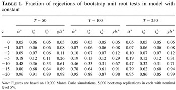
To illustrate the results in this section we have conducted a small Monte Carlo experiment for the case where the model contains a constant. For T = 50, T = 100, and T = 250, 10,000 samples were generated and the simulated observations calculated by the recursion (1) where α = 1 + c/T with c = 0,−1,−2,−5,−10,−15 and c = −20. The sequence {ε_t} consists of independent standard normal variables generated using the random number generator ran2 in Press, Teukolsky, Vetterling, and Flannery (1992).

For each sample, Y₁,…,Y_T, 5,000 bootstrap replications were constructed using (2) where ε₁*,…,ε_T* were sampled with replacement. Three sampling schemes were used: centered differences of the simulated observations, centered residuals from a fit using OLS in a model without intercept, and residuals from a fit using OLS in a model with intercept. In each bootstrap sample the following model was fitted by OLS:

In addition to

, two t-statistics were computed, one based on the variance estimator

, which we denote by t_α*, and another based on

, denoted by t_α**. The bootstrapped DF-GLS statistic is denoted by gls*.

Table 1 shows the fraction of the samples for which the various bootstrap tests rejected the null hypothesis of a unit root at the 5% nominal significance level. There are several interesting features worth mentioning. The first is that we did not notice any difference between the three sampling schemes. All resulted in the figures reported in Table 1. This is similar to what Li and Maddala (1996, 1997) report for the case where the model does not contain an intercept. Also, all bootstrap tests have correct size. Concerning the power, the ranking of the bootstrap tests is the same as one can expect from the asymptotic results of Figure 2 in Elliott et al. (1996). The bootstrap DF-GLS test is the most powerful, followed by the test based on

, the coefficient estimated by OLS. The studentized versions have least power. The two versions of the studentized test based on t_α* and t_α** have comparable properties, with the one using t_α* being slightly more powerful.

Fraction of rejections of bootstrap unit root tests in model with constant

The power of the bootstrap DF-GLS test increases as T grows, the power of the test based on

is fairly constant for the values of T considered, and the power of the studentized bootstrap test shows a slight decrease.

We have also computed the values of the ordinary unit root tests based on

and t_α using the critical values from Fuller (1996). The results are all within 0.01 of the corresponding figures of Table 1 corresponding to

tests, respectively. The asymptotic values corresponding to T = ∞ can be gleaned from Figure 2 in Elliott et al. and are close to those where T = 250.

5. PROOFS

Proof of Lemma 1. Consider first the case where

are sampled with replacement from the centered differences

. Given (Y₁,…,Y_T), ε_t*,t = 1,…,T are independent and identically distributed. The first property follows from

.

Furthermore

The process

, where [Ts] denotes the integer part of Ts, converges toward the Ornstein–Uhlenbeck process {σJ_c(s)}_0≤s≤1 in distribution in D[0,1] . This follows from Lemma 1 in Phillips (1987). As explained in Phillips and Perron (1988), therefore

converges in distribution toward

. Hence, the first term on the right-hand side of (17) tends to zero in P_c,T probability. The absolute value of the second term is bounded by

. By the weak law of large numbers

tends to σ² in P_c,T probability, which implies that Var*(ε_t*) → σ² in P_c,T probability.

We now consider the case where ε_t* = t = 1,…,T are sampled with replacement from the centered OLS residuals

. Because

. Now Var*(ε_t*) is given by a similar expression to (17) with c replaced by

. But us;

converges in P_c,T distribution, as shown by Phillips (1987), and hence is bounded in probability. Again Var*(ε_t*) → σ² in P_c,T probability. █

Proof of Lemma 2. The result follows from Theorem V.19 in Pollard (1984). The details can be found in Swensen (2002) for the case where c = 0. The generalization to convergence in P_c,T probability is straightforward using the convergence of the conditional moments proved in Lemma 1. █

Proof of Lemma 3. The lemma follows from Lemma 2 by an application of the continuous mapping theorem along the lines of Basawa et al. (1991b), (for a similar result, see also Heimann and Kreiss, 1996, p. 97). Here are the details. Using that

, we may write

as

The function

is continuous in the uniform metric in D[0,1] if g ≠ 0, and the continuous mapping theorem can be applied to the first term on the right-hand side of (18). As for the second term, for all

converges to zero in P_c,T probability. To verify that, let

. Then

and

. From (17) it follows that E*(ε₁*²) = Var*(ε₁*) → σ² in P_c,T probability and therefore E*(exp(isZ_T*)) → exp(isσ²) in probability. Hence

tends to zero in P_c,T probability. █

Proof of Lemma 4. We only consider the detrended case. The proof is essentially an adaptation of the arguments of the proof of Lemma A4 and Theorem 1.c in Elliott et al. (1996).

Let N_T be the diagonal matrix with diagonal elements

and 1 and Z_c = (z₁,z₂). Define Z as Z = Z_c N_T. Then

. But [(1/T)Z′Z]⁻¹ = D + A_T where D is a diagonal matrix with elements 1 and

along the diagonal and A_T = {a_ij,T} where a_ij,T = o(1),i,j = 1,2. Then

.

But

so that because

, an application of Lemma 2 and the continuous mapping theorem implies that the conditional distribution of

converges in P_c,T probability toward the distribution of (0,σβ)′ where

. Here we use that

Because

, it follows, again by Lemma 2 and the continuous mapping theorem because V₀(s,c) = W(s) − βs, that E*[f (S_T*^d)] → E [f (σV₀)] in P_c,T probability for all continuous f defined on D[0,1] . Arguing as in Lemma 3 will finish the proof. █