1 Introduction
In this article, we introduce a correlation number for pairs of well-behaved potentials over countable-state Markov shifts, defined through the study of their simultaneous orbital distributions. These dynamical results let us define a correlation number for pairs of cusped Hitchin representations. This correlation number quantifies the similarities of their marked length spectra and captures some rigidity properties.
Our dynamical results extend Lalley’s earlier work [Reference Lalley25] to non-compact settings. We derive the geometric counterparts through the symbolic coding of cusped Hitchin representations. A similar approach was successfully employed in previous work by Bray et al [Reference Bray, Canary, Kao and Martone5], where we established counting and equidistribution results for cusped Hitchin representations. In this article, we obtain a comparison of the growth rate of the marked length spectra of a pair of cusped Hitchin representations.
The primary motivation for this work stems from (higher rank) Teichmüller theory, especially from the study of geometrically meaningful diverging sequences of (cusped) Hitchin representations. Motivated by results of Dai and Martone [Reference Dai and Martone13], we wish to study the behavior of the correlation number along these sequences and interpret its limit. For example, given two sequences of hyperbolic structures converging to distinct points in the same stratum of the augmented Teichmüller space, as a consequence of Theorem 1.6, we can now define the correlation number of the limiting points and it would be interesting to compare it with the correlation number along the diverging sequences.
In the following subsections, we present our dynamical results first and then their applications to geometry.
1.1 General thermodynamical results
See §2 for precise definitions. Let
 $\Sigma ^{+}$
be a topologically mixing (one-sided) countable state Markov shift with big images and pre-images (BIP) property and consider two strictly positive, locally Hölder continuous, and independent potentials
 $f,g\colon \Sigma ^{+}\to \mathbb {R}$
. Let
 $\mathcal {A}$
denote the countable alphabet for
 $\Sigma ^+$
. Following [Reference Bray, Canary, Kao and Martone5], we say that a potential f has a strong entropy gap at infinity if the series
 $$ \begin{align*} Z_1(f,s)=\sum_{a\in\mathcal A}e^{-s\sup\{f(\underline{x})\colon \underline{x}\in\Sigma^+\text{ and } x_1=a\}} \end{align*} $$
has a finite critical exponent
 $d(f)>0$
and diverges when
 $s=d(f)$
. For the rest of this introduction, assume that f and g have strong entropy gaps at infinity,
 $\|f-g\|_\infty $
is finite, and set
 ${\mathbf {f}}=(f,g)$
.
We fix
 $\xi , m>0$
:
 $\xi $
is a (small) precision in our estimates, while m is an admissible slope, defined below in terms of the Manhattan curve of
 ${\mathbf {f}}$
. For any
 $t>0$
, let
 $I^2_{\xi , m}(t)$
denote the open rectangle
 $(t,t+\xi )\times (mt,mt+\xi )$
and for any
 $n\in \mathbb {Z}_{>0}$
, define
 $$ \begin{align*} \mathcal{M}(n,t)=\mathcal{M}(n,t;{\textbf{f},\xi,m):=\{\underline{x}\in\Sigma^{+}\colon\ \underline{x}\in {\mathrm{Fix}}^n,\ S_{n}{\textbf{f}(\underline{x})\in I^2_{\xi,m}(t)\}}}, \end{align*} $$
where
 $\mathrm {Fix}^n$
is the set of n-periodic words of
 $\Sigma ^+$
and
 $S_{n}{\mathbf {f}}$
denotes the pair of nth ergodic sums of
 $\mathbf {f}$
, that is,
 $$ \begin{align*} S_{n}{\textbf{f}}(\underline{x}):=\bigg(\sum_{k=1}^{n}f(\sigma^{k-1}(\underline{x})),\sum_{k=1}^{n}g(\sigma^{k-1}(\underline{x}))\bigg). \end{align*} $$
The first goal of this article is to study the growth rate as t goes to infinity of
 $$ \begin{align*} M(t;{\textbf{f},m,\xi):=\sum_{n}\frac{1}{n}\#\mathcal{M}(n,t;{\textbf{f},m,\xi)}}. \end{align*} $$
Theorem 1.1. For any admissible slope m,
 $M(t;{\mathbf {f}},m,\xi )$
grows exponentially. Specifically, the limit
 $$ \begin{align*} \alpha_{\mathbf{f}}(m) := \lim_{t\to\infty} \frac{1}{t} \log M(t;{\mathbf{f}},m,\xi) \end{align*} $$
exists and, moreover,
 $0 < \alpha _{\mathbf {f}}(m) < \infty .$
In what follows, we examine properties of the exponential growth rate
 $\alpha _{\mathbf {f}}(m)$
of
 $M(t;{\mathbf {f}},m,\xi )$
, which we call the correlation number of
 $\mathbf {f}$
and m. A cylinder p is a subset of
 $\Sigma ^+$
consisting of words sharing an initial string of length
 $|p|\in \mathbb N$
. Our second result provides a more precise asymptotic growth estimate for
 $$ \begin{align*} M_{p}(t;{\textbf{f},m,\xi):=\sum_{n}\frac{1}{n}\#\mathcal{M}_{p}(n,t;{\textbf{f},m,\xi)}}, \end{align*} $$
where, for any cylinder p, we write
 $\mathcal {M}_{p}(n,t;{\mathbf {f},m,\xi )\colon =\mathcal {M}(n,t;{\textbf {f},m,\xi )\cap p}}$
. Notably, we obtain a finer asymptotic estimate when we restrict to a cylinder.
Theorem 1.2. For any admissible slope m and any cylinder p, there exist constants
 $C_{1}(p)$
and
 $C_{2}(p)$
such that
 $$ \begin{align*} C_{1}(p) \leq \lim_{t \to \infty} \frac{t^{{3}/{2}}}{e^{\alpha_{\mathbf{f}}(m)t}} M_{p}(t;{\mathbf{f}},m,\xi) \leq C_{2}(p) \end{align*} $$
and
 $$ \begin{align*} \lim_{|p| \to \infty} \frac{C_{1}(p)}{C_{2}(p)} = 1. \end{align*} $$
By restricting our focus to the counting problem on cylinders, Theorem 1.2 provides an estimate for the local asymptotic expansion of the orbital distribution with respect to
 $\mathbf {f}$
and m. Unlike in the compact case, the global asymptotic expansion does not immediately follow from the local version. While we expect that the global asymptotic expansion also holds, we would need a stronger version of Lemma 5.4 to establish it. See Remark 6.4 for more details. However, let us note that the local asymptotic expansion suffices for our main applications.
Next, we explicitly relate the growth rate
 $\alpha _{\mathbf {f}}(m)$
to the Manhattan curve, an important dynamical object associated with orbital distribution problems for
 $\mathbf {f}$
, first introduced by Burger in [Reference Burger7]. Let P denote the topological pressure associated with
 $\Sigma ^+$
. We recall (see §2.5 for more details) that the Manhattan curve of
 $\mathbf {f}$
is the curve
 $$ \begin{align*} \mathcal{C}(\mathbf{f}) = \{(a,b) \in \mathbb{R}^{2} \colon P(-af - bg) = 0,\ a \geq 0,\ b \geq 0,\ a + b> 0\}. \end{align*} $$
By the analyticity properties of the pressure function P and [Reference Bray, Canary, Kao and Martone5, Theorem C], we know that the Manhattan curve
 $\mathcal {C}(\mathbf {f})$
can be parameterized by
 $(s, q(s))$
, where
 $q = q(s)$
is a real analytic function for
 $s \in [0, \delta _f]$
. Here,
 $\delta _f$
is the unique value for which
 $P(-\delta _f f) = 0$
. The slope of the normal to the Manhattan curve at the point
 $(s, q(s))$
is given by
 ${m(s) = -1 / q'(s)}$
. We then say that
 $m = m(s)$
is an admissible slope and we denote by
 $\mathcal {S}(\mathbf {f})$
the set of admissible slopes. In particular, note that
 $m_* = \delta _f / \delta _g \in \mathcal {S}(\mathbf {f})$
(see Theorem 2.14).
Given an admissible slope m, we denote by
 $(a_m, b_m)$
the point on
 $\mathcal {C}(\mathbf {f})$
where the slope of the normal equals m. With this notation, we can define the quantity
 $$ \begin{align*} H_{\mathbf{f}}(m) := a_m + m \cdot b_m. \end{align*} $$
The following result shows that
 $H_{\mathbf {f}}(m)$
equals the correlation number of
 $\mathbf {f}$
and m.
Theorem 1.3. If
 $m\in \mathcal {S}(\mathbf {f})$
is an admissible slope, then
 $$ \begin{align*} \alpha_{\mathbf{f}}(m)=H_{\mathbf{f}}(m). \end{align*} $$
Using the convexity of the Manhattan curve and the above results, we derive a rigidity result for the special admissible slope
 $m_*=\delta _f/\delta _g$
.
Corollary 1.4. (Correlation number rigidity)
For
 $m_*=\delta _f/\delta _g$
, we have
 $$ \begin{align*} \alpha_{\mathbf{f}}(m_*)=H_{\mathbf{f}}(m_*)\leq\delta_f. \end{align*} $$
Moreover, the equality holds if and only if
 $m_*S_{n}f(\underline {x})=S_{n}g(\underline {x})$
for all
 $\underline {x}\in \mathrm {Fix}^{n}.$
Another interesting dynamical growth rate associated with
 $\mathbf {f}$
is
 $h_{(\alpha , \beta )}^{\mathrm {BS}}({\mathbf {f}})$
, the
 $(\alpha ,\beta )$
-Bishop–Steger entropy, defined for
 $\alpha , \beta> 0$
as
 $$ \begin{align*} h_{(\alpha, \beta)}^{\mathrm{BS}}({\textbf{f}}) := \lim_{t \to \infty} \frac{1}{t} \log \sum_{n} \frac{1}{n} \#\{ \underline{x}\in {\mathrm{ Fix}}^n \colon \alpha S_{n} f(\underline{x}) + \beta S_{n} g(\underline{x}) \leq t \}. \end{align*} $$
Our last result in the symbolic setting relates the Bishop–Steger entropy with the correlation number.
Theorem 1.5. Let
 $m \in \mathcal {S}(\mathbf {f})$
be an admissible slope. Then,
 $$ \begin{align*} \frac{H_{{\textbf{f}}}(m)}{\alpha + m\beta} \leq h_{(\alpha, \beta)}^{\mathrm{BS}}({\textbf{f}}), \end{align*} $$
with equality if and only if m is the unique slope satisfying
 $a_{m}/b_{m} = \alpha /\beta $
.
1.2 Application to cusped Hitchin representations
We apply the results above to pairs of cusped Hitchin representations. See §7 for details. Let
 $\Gamma $
be a torsion-free geometrically finite Fuchsian group which is not convex-cocompact. The recurrent portion of the geodesic flow on
 $T^1(\mathbb {H}^2/\Gamma )$
can be coded by a topologically mixing countable states Markov shift
 $\Sigma ^+$
with BIP. In particular, there is a map
 $G\colon \mathrm {Fix}^n\to \Gamma $
such that if
 $\gamma \in \Gamma $
is hyperbolic, then it is conjugated to
 $G(\underline {x})$
for some n and a unique up to shift
 $\underline {x}\in \mathrm {Fix}^n$
.
A representation
 $\rho \colon \Gamma \to \textsf {SL}(d,\mathbb R)$
is cusped Hitchin if there exists a continuous,
 $\rho $
-equivariant, positive map from the limit set of
 $\Gamma $
to the space of complete flags in
 $\mathbb R^d$
. Using a Lie theoretic construction, a cusped Hitchin representation together with a choice of a non-zero positive linear combination
 $\phi $
of the simple roots of
 $\textsf {SL}(d,\mathbb {R})$
determines a length function
 $\ell ^\phi _\rho \colon \Gamma \to \mathbb R_{\geq 0}$
, which is constant on the conjugacy class
 $[\gamma ]\in [\Gamma ]$
of an element
 $\gamma \in \Gamma $
. Then, for any cusped Hitchin representation
 $\rho \colon \Gamma \to \textsf {SL}(d,\mathbb {R})$
and any such
 $\phi $
, there exists a strictly positive locally Hölder continuous potential
 $\tau _\rho ^\phi $
with a strong entropy gap at infinity and such that
 $$ \begin{align*} \tau_\rho^\phi(\underline{x})=\ell^\phi_\rho(G(\underline{x})) \end{align*} $$
for any
 $\underline {x}\in \mathrm {Fix}^n$
. Moreover, given another cusped Hitchin representation
 $\eta \colon \Gamma \to \textsf {SL}(d,\mathbb {R})$
, then
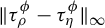 $\|\tau _\rho ^\phi -\tau _\eta ^\phi \|_\infty $
is finite and
 $\tau _\rho ^\phi $
and
 $\tau _\eta ^\phi $
are independent unless
 $\eta =\rho ,(\rho ^{-1})^\top $
, see Lemma 7.3.
Recall that for a cusped Hitchin representation
 $\rho $
and a non-zero positive linear combination
 $\phi $
of the simple roots of
 $\textsf {SL}(d, \mathbb {R})$
, we can define
 $\delta _\phi (\rho )$
, the
 $\phi $
-topological entropy, as
 $\delta _{\tau ^\phi _\rho }$
, the entropy of the corresponding potential
 $\tau ^\phi _\rho $
. Furthermore, for a pair of cusped Hitchin representations
 $(\rho , \eta )$
and a given
 $\phi $
, we can define the Manhattan curve
 $\mathcal {C}^\phi (\rho , \eta )$
by
 $\mathcal C(\tau ^\phi _\rho , \tau ^\phi _\eta )$
. (See [Reference Bray, Canary, Kao and Martone5, Corollaries 1.3 and 1.4] for more details.) Thus, we can apply our results from symbolic dynamics to obtain the following theorem.
Theorem 1.6. Let
 $\rho ,\eta \colon \Gamma \to \textsf {SL}(d,\mathbb {R})$
be cusped Hitchin representations such that
 $\eta \neq \rho ,(\rho ^{-1})^\top $
and let
 $\phi $
be a non-zero positive linear combination of the simple roots of
 $\textsf {SL}(d,\mathbb {R})$
. Let m be an admissible slope for the Manhattan curve
 $\mathcal C^\phi (\rho ,\eta )$
. Then,
 $$ \begin{align*} \lim_{t\to \infty}\frac{1}{t}\log\{[\gamma]\in[\Gamma]\colon (\ell^\phi_\rho(\gamma),\ell^\phi_\eta(\gamma))\in I^2_{\xi, m}(t)\}=:H^\phi_{(\rho,\eta)}(m)=a_m+m\cdot b_m, \end{align*} $$
where
 $H^{\phi }_{(\rho ,\eta )}(m)$
is the correlation number of
 $(\rho ,\eta )$
and
 $\phi $
, and
 $(a_m,b_m)$
is the point
 $\mathcal {C}^\phi (\rho ,\eta )$
where the slope of the normal equals m.
The following rigidity result follows immediately from Theorem 1.6, Corollary 1.4, and [Reference Bray, Canary, Kao and Martone5, Corollary 1.5].
Corollary 1.7. (Correlation number rigidity II)
Under the same assumptions as in Theorem 1.6, for
 $m_* = \delta _\phi (\rho ) / \delta _\phi (\eta )$
, we have
 $$ \begin{align*} H^\phi_{(\rho,\eta)}(m_*) \leq \delta_\phi(\rho). \end{align*} $$
Moreover, equality holds if and only if
 $m_* \ell ^\phi _\rho (\gamma ) = \ell ^\phi _\eta (\gamma )$
for all
 $\gamma \in \Gamma $
.
Similarly, we can define the
 $(\alpha , \beta )$
-Bishop–Steger entropy of
 $\phi $
,
 $\rho $
, and
 $\eta $
as
 $h_{(\alpha , \beta )}^{\phi }(\rho ,\eta ):= h_{(\alpha , \beta )}^{\mathrm {BS}}(\tau ^\phi _\rho , \tau ^\phi _\eta ).$
Then, Theorem 1.5 can be rewritten as follows.
Theorem 1.5 *
Let m be an admissible slope. Then,
 $$ \begin{align*} \frac{H^\phi_{(\rho,\eta)}(m)}{\alpha + m\beta} \leq h_{(\alpha, \beta)}^{\phi}(\rho,\eta), \end{align*} $$
with equality if and only if m is the unique slope satisfying
 $a_m / b_m = \alpha / \beta $
.
1.3 Outline of the paper and main steps
The approach in this paper combines ideas from [Reference Bray, Canary, Kao and Martone5, Reference Lalley25]. The results in [Reference Bray, Canary, Kao and Martone5] rely on a renewal theorem, which is not available when studying simultaneous orbital distribution problems. For this reason, we follow Lalley’s strategy from the compact case [Reference Lalley25] and use Fourier analysis to study the asymptotic behavior of the simultaneous orbital distribution of a pair of potentials.
Lalley’s method involves two key steps. The first step consists of converting the counting problem into estimates on thermodynamical quantities. The second step uses Fourier analysis on these quantities to derive the relevant asymptotic expansions. The simultaneous orbital growth problem studied in this paper is a refinement of the single-orbital growth problem treated in [Reference Bray, Canary, Kao and Martone5]. To extend Lalley’s method to the non-compact setting, we build upon the framework in [Reference Bray, Canary, Kao and Martone5] to establish more delicate estimates that we can then use to perform the two steps as above.
In what follows, we outline the main steps of each section. Section 2 gathers essential background results and definitions from the thermodynamic formalism and the entropy gaps at infinity introduced in [Reference Bray, Canary, Kao and Martone5]. In §3, we begin our study of the correlation number
 $ H_{\mathbf {f}}(m) $
and establish the rigidity results given in Corollary 1.4 and Theorem 1.5. Section 4 reformulates the orbit counting problem by linking it to the transfer operator, enabling the application of tools from thermodynamic formalism. In §5, we derive a priori estimates for the counting problem over countable Markov shifts, giving an upper bound for the simultaneous orbital growth. Section 6 uses Fourier analysis and the saddle point method to establish a local asymptotic expansion, providing a lower bound for the simultaneous orbital growth and thereby proving Theorems 1.1, 1.2, and 1.3. In §7, we review key aspects of the theory of cusped Hitchin representations and establish Lemma 7.3, which allows us to apply our main dynamical results in this context, leading to the proof of Theorem 1.6. Finally, in Appendices A and B, we provide proofs of Theorem 2.7 and Proposition 6.11, which are known to experts, but we were not able to find in the available literature.
1.4 Historical remarks
Orbital distribution has long been a central theme in ergodic geometry. A key early milestone in this field is the prime orbit theorem (see, for example, the foundational works of Huber, Margulis, Lalley, Parry, and Pollicott [Reference Huber18, Reference Lalley27, Reference Margulis29, Reference Parry and Pollicott31]), which establishes a connection between the growth rate of closed orbits and topological entropy. Lalley’s pioneering work [Reference Lalley25, Reference Lalley26] introduces probabilistic perspectives to study orbital distribution problems within compact settings. Building on this foundation, along with earlier contributions by the authors [Reference Bray, Canary, Kao and Martone5, Reference Kao19, Reference Kao20], our work extends Lalley’s results to a large class of countable Markov shifts.
Lalley’s results in [Reference Lalley25] initiated further investigations into correlation numbers, which Sharp [Reference Sharp43] later explored through a different approach. Lalley’s subsequent work [Reference Lalley26] focused on counting closed orbits within specific homology classes, drawing inspiration from Phillips and Sarnak [Reference Phillips and Sarnak33], and Katsuda and Sunada [Reference Katsuda and Sunada22]. This problem was further studied by Pollicott and Sharp [Reference Pollicott34, Reference Sharp42] using a zeta function approach. Babillot and Ledrappier [Reference Babillot and Ledrappier2] later provided a unified framework for these two closely related counting problems in compact hyperbolic flows.
Schwartz and Sharp [Reference Schwartz and Sharp41] used Lalley’s work [Reference Lalley25] to define and examine the correlation of length spectra of two hyperbolic structures on a closed surface. Pollicott and Sharp [Reference Pollicott and Sharp35, Reference Pollicott and Sharp36] further analyzed a related correlation number, defined relative to word length. Glorieux [Reference Glorieux17] studied correlation numbers with slope from the perspective of globally hyperbolic maximally Cauchy-compact anti-de Sitter manifolds. Dai and the second author [Reference Dai and Martone13] extended Schwartz and Sharp’s approach to pairs of Hitchin representations. Chow and Oh [Reference Chow and Oh11, Reference Chow and Oh12] recently developed a new approach and generalized these results to tuples of Anosov groups.
Cusped Hitchin representations are examples of positive representations in the sense of Fock and Goncharov [Reference Fock and Goncharov16]. Canary, Zhang, and Zimmer [Reference Canary, Zhang and Zimmer9] establish several of their geometric properties, which extend results on Anosov representations. Bray et al developed dynamical aspects of this theory in [Reference Bray, Canary, Kao and Martone5, Reference Bray, Canary, Kao and Martone6]. We refer to [Reference Canary8] for a survey on (cusped) Hitchin representations.
In the non-convex cocompact setting, constrained counting problems remain less developed. Epstein [Reference Epstein15] studied the counting of orbits in given homology classes for finite-volume hyperbolic manifolds, while Babillot and Peigné [Reference Babillot and Peigné3] extended these results to certain infinite-volume hyperbolic manifolds with cusps. To the best of our knowledge, no other results on correlation numbers exist in non-convex cocompact settings, apart from Theorems 1.1 and 1.2. Moreover, these two results partially answer open question no. 7 listed on [Reference Paulin, Pollicott and Schapira32, p. 11].
Theorem 1.3 generalizes [Reference Sharp43, Theorem 1] and [Reference Glorieux17, Theorem 3.25] (with slopes) for convex cocompact Fuchsian representations, as well as [Reference Dai and Martone13, Theorem 6.14] for Hitchin representations. Corollary 1.4 draws inspiration from the intersection number rigidity result in [Reference Bray, Canary, Kao and Martone5, Corollary 1.5]. Finally, Theorem 1.5 studies the relation between the correlation number and (generalized) Bishop–Steger entropy, extending [Reference Glorieux17, Theorem 3.15] for convex cocompact Fuchsian representations to cusped Hichin representations.
2 Background
2.1 Markov shifts
A countable state Markov shift is the data of a countable alphabet
 $\mathcal A$
, a transition matrix
 $\mathbb T=(t_{ab})\in \{0,1\}^{\mathcal A\times \mathcal A}$
, the set of words
 $$ \begin{align*} \Sigma^+=\{\underline{x}=(x_n)\in\mathcal A^{\mathbb Z_{>0}}\colon t_{x_nx_{n+1}}=1\}, \end{align*} $$
and the left-shift
 $\sigma \colon \Sigma ^+\to \Sigma ^+$
defined by
 $\sigma ((x_n))=(x_{n+1})$
. The countable state Markov shift is: (i) topologically mixing if for any letters
 $a,b\in \mathcal A$
, there exists
 $N=N(a,b)$
such that for any
 $n> N$
, there exists a word
 $\underline {x}\in \Sigma ^+$
with
 $x_1=a$
and
 $x_n=b$
; (ii) has BIP, short for big images and pre-images property, if there exists a finite subset
 $\mathcal B$
of the alphabet
 $\mathcal A$
such that for any
 $a\in \mathcal A$
, there exist letters
 $b_p,b_s\in \mathcal B$
such that
 $t_{b_pa}=t_{ab_s}=1$
. For the rest of this section, we fix a topologically mixing, countable state Markov shift with BIP which, with a slight abuse of notation, we denote by
 $\Sigma ^+$
. Furthermore, we equip
 $\Sigma ^+$
with the metric
 $d(\underline {x},\underline {y})=e^{-\inf \{n:\ x_n\neq y_n\}}$
.
For any
 $k\in \mathbb Z_{>0}$
, a k-cylinder is a non-empty subset
 $p\subset \Sigma ^+$
defined by the property
 $$ \begin{align*} \underline{x},\underline{y}\in p \iff x_i=y_i\quad \text{for all } i=1,\ldots,k. \end{align*} $$
Denote by
 $\Lambda _k$
the set of k-cylinders.
2.2 Potentials, entropy gaps, and pressure
A potential is a continuous function
 $f\colon \Sigma ^+\to \mathbb K$
, where
 $\mathbb K=\mathbb R$
or
 $\mathbb C$
equipped with the norm
 $|\cdot |$
. The nth ergodic sum of f is the potential
 $$ \begin{align*} S_nf(\underline{x})=\sum_{i=0}^{n-1}f(\sigma^i(\underline{x})). \end{align*} $$
A potential
 $f\colon \Sigma ^+\to \mathbb K$
is locally Hölder continuous (or
 $\beta $
-locally Hölder continuous with constant A) if there exist
 $A,\beta>0$
such that
 $$ \begin{align*} |f(\underline{x})-f(\underline{y})|<Ad(\underline{x},\underline{y})^\beta \end{align*} $$
whenever
 $x_1=y_1$
. We denote by
 $\mathcal F_\beta $
(respectively
 $\mathcal F_\beta (\mathbb C)$
) the space of
 $\beta $
-locally Hölder continuous potentials valued in
 $\mathbb R$
(respectively
 $\mathbb C$
) equipped with the norm
 $$ \begin{align*} \|\phi\|_{\beta}=\|\phi\|_{\infty}+\text{Lip}(\phi)\quad \text{where Lip }(\phi):=\sup \bigg\{\frac{|\phi(\underline{x})-\phi(\underline{y})|}{d(\underline{x},\underline{y})^\beta} \colon\ \underline{x}\neq \underline{y},\ x_1=y_1\bigg\}. \end{align*} $$
Then, let
 $\mathcal F^b_\beta (\mathbb C)$
denote the subspace of bounded potentials and let
 $\mathcal B(\mathcal F^b_\beta (\mathbb C))$
be the space of bounded operators on
 $\mathcal F^b_\beta (\mathbb C)$
equipped with the operator norm
 $$ \begin{align*} \|\mathcal L\|_{\mathrm{{op}}}=\sup\bigg\{\frac{\|\mathcal L(\phi)\|_\beta}{\|\phi\|_\beta}:\ \phi\in \mathcal F^b_\beta(\mathbb C)\bigg\}. \end{align*} $$
Note that
 $(\mathcal F^b_\beta (\mathbb C),\|\cdot \|_\beta )$
and
 $(\mathcal B(\mathcal F^b_\beta (\mathbb C)),\|\cdot \|_{\mathrm {{op}}})$
are Banach spaces.
Let
 $f\colon \Sigma ^+\to \mathbb R$
be locally Hölder continuous and set
 $ S(f,a)=\sup \{f(\underline {x})\colon \underline {x}\in \Sigma ^{+}, x_{1}=a\}.$
Then, recall from the introduction that f has a strong entropy gap at infinity if the series
 $$ \begin{align*} Z_{1}(f,s)=\sum_{a\in\mathcal{A}}e^{-sS(f,a)} \end{align*} $$
has a finite critical exponent
 $d(f)>0$
and diverges when
 $s=d(f)$
.
Let
 $\mathcal M_\sigma $
denote the space of shift-invariant probability measures on
 $\Sigma ^+$
and, for any
 $\mu \in \mathcal M_\sigma $
, let
 $h_\sigma (\mu )$
denote the measure-theoretic entropy of
 $\sigma $
with respect to
 $\mu $
. The (topological) pressure of the locally Hölder continuous potential f is
 $$ \begin{align*} P(f)=\sup\bigg\{h_\sigma(\mu)+\int_{\Sigma^+}f\,d\mu\colon \mu\in\mathcal M_\sigma\text{ and }-\int_{\Sigma^+}f\, d\mu<\infty\bigg\}. \end{align*} $$
An equilibrium state for a potential f is a
 $\sigma $
-invariant Borel probability measure
 $\mu $
on
 $\Sigma ^+$
such that
 $$ \begin{align*} P(f) = h_\sigma(\mu) + \int_{\Sigma^+} f \, d\mu. \end{align*} $$
A Gibbs state for f is a Borel probability measure
 $\nu $
on
 $\Sigma ^+$
for which there exists a constant
 $Q> 1$
such that
 $$ \begin{align*} \frac{1}{Q} \leq \frac{e^{S_n f(\underline{x}) - nP(f)}}{\nu(p)} \leq Q \end{align*} $$
for any n-cylinder p and any
 $\underline {x}$
in p.
The Gibbs states and equilibrium states of potentials with good regularity (if they exist) are closely related. Specifically, we have the following result.
Theorem 2.1. (Mauldin and Urbański [Reference Mauldin and Urbański30, Theorem 2.2.9], Sarig [Reference Sarig40, Theorem 4.9])
Let
 $\Sigma ^+$
be a topologically mixing, countable state Markov shift with BIP. If f is a real-valued, locally Hölder continuous potential with finite pressure, then f admits a unique shift-invariant Gibbs state
 $\mu _f$
. Moreover, if
 $-\int f \, d\mu _f < \infty $
, then
 $\mu _f$
is the unique equilibrium state for f.
Two locally Hölder continuous potentials f and g are (Livšic) cohomologous if there exists a locally Hölder continuous potential h such that
 $f-g=h-h\circ \sigma $
. The real-valued potential f is strictly positive if there exists a constant
 $B> 0$
such that
 $f(\underline {x})> B$
for all
 $\underline {x} \in \Sigma ^+$
.
Remark 2.2. Several of the results from [Reference Bray, Canary, Kao and Martone5] used in this work hold more generally for eventually positive potentials. However, in this paper, we will need the stronger hypothesis of strict positivity, as in [Reference Bray, Canary, Kao and Martone5, Theorem C]. We note that, by [Reference Bray, Canary, Kao and Martone5, Lemma 3.2], any eventually positive locally Hölder continuous potential with a strong entropy gap at infinity is cohomologous to a strictly positive potential with the same properties.
A potential
 $f\colon \Sigma ^+\to \mathbb R$
is arithmetic if the additive subgroup of
 $\mathbb R$
generated by
 $\{S_nf(\underline {x})\colon \underline {x}\in \mathrm {Fix}^n,\ n\in \mathbb N\}$
is cyclic. Two potentials are independent if
 $af+bg$
is arithmetic only if
 $a=b=0$
. Note that if f and g are independent, then each one of them is non-arithmetic.
Assumptions 2.3. From now on through the paper, we assume that
 $\Sigma ^{+}$
is a topologically mixing, countable state Markov shift with BIP, and let
 $f,g\colon \Sigma ^+\to \mathbb R$
denote strictly positive locally Hölder continuous potentials with strong entropy gaps at infinity such that
 $\|f-g\|_\infty $
is finite. We often write
 $\mathbf {f}$
for the pair
 $(f,g)$
.
Remark 2.4.
-
(1) When clear from context, our notation will not highlight the dependence on the fixed pair of potentials
 $\mathbf {f}$
.
-
(2) Assuming that
$\|f-g\|_\infty $
is finite and f has a strong entropy gap at infinity guarantees that the same property holds for g. However, we explicitly assume that g has a strong entropy gap at infinity to ease exposition.


2.3 Transfer operators
We are interested in certain weighted sums of f and g that have finite pressure. More specifically, we will consider weights in the set
 $$ \begin{align} D=D(\mathbf{f})&:=(\{(z_{1},z_{2})\in\mathbb{R}^{2}\colon z_1\leq 0,z_2\leq 0,z_1+z_2<0\}\nonumber\\ &\qquad\cup \{(z_{1},z_{2})\in\mathbb{R}^{2}\colon z_1> 0,z_2<0,z_1c(f)+z_2(c(f)-A)<0\}\nonumber\\ &\qquad\cup \{(z_{1},z_{2})\in\mathbb{R}^{2}\colon z_1<0,z_2>0,z_1(c(g)-A)+z_2c(g)<0\})\nonumber\\ &\quad\cap\{(z_{1},z_{2})\in\mathbb{R}^{2}\colon d(-z_{1}f-z_{2}g)<1\}, \end{align} $$
where
 $A>0$
is such that
 $\|f-g\|_{\infty }=A<\infty $
,
 $c(f)=\inf _{\Sigma ^+}f>0$
, and
 $c(g)=\inf _{\Sigma ^+}g>0$
. Notice that for any
 $(z_{1},z_{2})\in D$
, the potential
 $-(z_{1}f+z_{2}g)$
is locally Hölder continuous, strictly positive, and with strong entropy gap at infinity. In particular, [Reference Bray, Canary, Kao and Martone5, Lemma 3.3(1)] implies that
 $D\subset \{(z_{1},z_{2})\in \mathbb {R}^{2}\colon P(z_{1}f+z_{2}g)<\infty \}$
. We now list some important properties of the weights in D.
Proposition 2.5. For any
 $(z_{1},z_{2})\in D$
, the following holds.
-
(1) The potential
$z_{1}f+z_{2}g$
has a unique equilibrium state
$\mu _{z_{1}f+z_{2}g}$
. -
(2) The potentials
$f,g$
are in
$L^{n}(\mu _{z_{1}f+z_{2}g})$
for all
$n\in \mathbb {N}.$
-
(3) D is an open set in
$\mathbb R^2$
.


Proof. The first assertion follows from the assumption
 $d(-z_1f-z_2g)<1$
together with [Reference Bray, Canary, Kao and Martone5, Lemma 3.4]. For the second assertion, since
 $-(z_{1}f+z_{2}g)$
has a strong entropy gap at infinity, the series
 $$ \begin{align*} Z_{1}(-z_{1}f-z_{2}g,s)=\sum_{a\in\mathcal{A}}e^{-sS(-z_{1}f-z_{2}g,a)} \end{align*} $$
converges for all
 $s>d(-(z_{1}f+z_{2}g)).$
Since we assume
 $(z_1,z_2)\in D$
, we can find
 $\epsilon>0$
small enough such that
 $1-\epsilon>d(-(z_{1}f+z_{2}g))$
, and thus,
 $$ \begin{align*} \sum_{a\in\mathcal{A}}e^{-(1-\epsilon)S(-z_{1}f-z_{2}g,a)}<\infty. \end{align*} $$
Then,
 $$ \begin{align*} \infty>\sum_{a\in\mathcal{A}}e^{-(1-\epsilon)S(-z_{1}f-z_{2}g,a)} & =\sum_{a\in\mathcal{A}}e^{-S(-z_{1}f-z_{2}g,a)}e^{\epsilon S(-z_{1}f-z_{2}g,a)}\\ & =\sum_{a\in\mathcal{A}}e^{-S(-z_{1}f-z_{2}g,a)}\sum_{n\geq1}\frac{\epsilon^{n}}{n!}(S(-z_{1}f-z_{2}g,a))^{n}\\ & =\sum_{n\geq1}\sum_{a\in\mathcal{A}}\frac{\epsilon^{n}}{n!}(S(-z_{1}f-z_{2}g,a))^{n}e^{-S(-z_{1}f-z_{2}g,a)}, \end{align*} $$
where we can swap the series because
 $(z_1,z_2)\in D$
,
 $-z_1f-z_2g$
is strictly positive; thus, guaranteeing absolute convergence. It follows that for all
 $n\in \mathbb {N}$
,
 $$ \begin{align*} \sum_{a\in\mathcal{A}}(S(-z_{1}f-z_{2}g,a))^{n}e^{-S(-z_{1}f-z_{2}g,a)}<\infty. \end{align*} $$
Now, for all
 $a\in \mathcal A$
, let
 $[a]$
denote the cylinder of words starting with the letter a and, for any locally Hölder continuous potential h, let
 $I(h,a)$
denote the infimum of
 $\{h(\underline {x})\colon \underline {x}\in [a] \}$
. By the Gibbs property of
 $\mu _{z_1f+z_2g}$
, we know that there exists
 $Q>1$
such that
 $$ \begin{align*} e^{-I(-z_{1}f-z_{2}g,a)}= e^{S(z_{1}f+z_{2}g,a)}\geq\frac{e^{P(z_{1}f+z_{2}g)}}{Q}\mu_{z_{1}f+z_{2}g}([a]). \end{align*} $$
Hence,
 $$ \begin{align*} & 0<\int|-z_{1}f-z_{2}g|^{n}\ d\mu_{z_{1}f+z_{2}g}\\ &\leq\frac{Q}{e^{P(z_{1}f+z_{2}g)}}\sum_{a\in\mathcal{A}}(S(-z_{1}f-z_{2}g,a))^{n}e^{-I(-z_{1}f-z_{2}g,a)}\\ &\leq \frac{Q}{e^{P(z_{1}f+z_{2}g)}}\sum_{a\in\mathcal{A}}(S(-z_{1}f-z_{2}g,a))^{n}e^{-S(-z_{1}f-z_{2}g,a)+A}<\infty, \end{align*} $$
where we used that the potential
 $-z_1f-z_2g$
is locally Hölder continuous to see that
 $$ \begin{align*} |I(-z_{1}f-z_{2}g,a)-S(-z_{1}f-z_{2}g,a)|<A \end{align*} $$
for some uniform constant
 $A>0$
. From here, we deduce that
 $f,g\in L^{n}(\mu _{z_{1}f+z_{2}g})$
for all
 $n\in \mathbb {N}$
.
The last assertion is an immediate consequence of the formula
 $$ \begin{align*}d(-z_1f-z_2g){}=\frac{d(f)}{-(z_1+z_2)}\end{align*} $$
established in the proof of [Reference Bray, Canary, Kao and Martone5, Theorem C*].
Consider a locally Hölder continuous potential
 $h\colon \Sigma ^+\to \mathbb K$
. The transfer operator
 $\mathcal {L}_{h}$
of h (also known as the Ruelle–Perron–Frobenius operator) is defined by
 $$ \begin{align*} \mathcal{L}_{h}\phi(\underline{x})=\sum_{\underline{y}\in\sigma^{-1}(\underline{x})}e^{h(\underline{y})}\phi(\underline{y}), \end{align*} $$
where
 $\phi \colon \Sigma ^+\to \mathbb K$
is a bounded locally Hölder continuous potential. The eigenvalues and eigenvectors of the transfer operator are related to the pressure and equilibrium states as follows.
Theorem 2.6. (Mauldin and Urbański [Reference Mauldin and Urbański30, Corollary 2.7.5], Sarig [Reference Sarig40, Theorem 4.9])
If
 $u :\Sigma ^+\to \mathbb R$
is locally Hölder continuous,
 $P(u)<+\infty $
and
 $\sup u<+\infty $
, then there exist unique probability measures
 $\mu _u$
and
 $\nu _u$
on
 $\Sigma ^+$
and a positive function
 $h_u:\Sigma ^+\to \mathbb R$
so that
 $$ \begin{align*}\mu_u=h_u\nu_u,\quad \mathcal L_uh_u=e^{P(u)}h_u\quad\text{and}\quad \mathcal L_u^*\nu_u=e^{P(u)}\nu_u.\end{align*} $$
Moreover,
 $h_u$
is bounded away from both
 $0$
and
 $+\infty $
, and
 $\mu _u$
is an equilibrium state for u.
We will be interested in complex analytic perturbations of the transfer operator. To this end, consider the complex domain
 $$ \begin{align*} \overline{D}=\overline{D}(\mathbf{f}):=\{(z,w)\subset\mathbb{C}\times\mathbb{C}:\ (\Re{z},\Re{w})\in D\},\end{align*} $$
which contains
 $D=D(\mathbf {f})$
.
Theorem 2.7. (Holomorphicity)
The map
 $\overline D\to \mathcal {B}(\mathcal {F}_{\beta }^{b}(\mathbb {C}))$
defined by
 $(z,w)\mapsto \mathcal {L}_{zf+wg}$
is holomorphic.
Proof. The proof follows from [Reference Sarig39, Proposition 2(3)] with some minor modifications and simplifications. For the sake of completeness and readability, we present the argument in Appendix A.
We recall the well-known analytic perturbation theorem (cf. for example, [Reference Kato21], [Reference Parry and Pollicott31, Proposition 4.6], [Reference Sarig40, Theorem 5.6], or [Reference Kloeckner24, Theorem]).
Theorem 2.8. (Analytic perturbation theorem)
Let X be a complex, (respectively real) Banach space and
 $\mathcal {B}(X)$
be the space of bounded linear operators acting on X endowed with the operator norm. If
 $\mathcal {L}_{0}\in \mathcal {B}(X)$
has a simple isolated eigenvalue, then there is an open neighborhood V of
 $\mathcal L_{0}$
such that every
 $\mathcal {L}\in V$
has an eigenvalue
 $\unicode{x3bb} _{\mathcal L}$
close to
 $\unicode{x3bb} _{0}$
. The map
 $\unicode{x3bb} \colon V\to \mathbb {C}$
(respectively
 $\mathbb {R}$
) is analytic,
 $\mathcal {L}$
does not have other eigenvalues near
 $\unicode{x3bb} _0$
, and there is another analytic map
 $u:V\to X$
such that
 $u_{\mathcal L}$
is an eigenvector of
 $\mathcal {L}$
for
 $\unicode{x3bb} _{\mathcal {L}}$
.
The following corollary is a consequence of the analytic perturbation theorem discussed above, which can be viewed as a complex version of the Ruelle–Perron–Frobenius theorem. See, for example, Sarig [Reference Sarig40, Theorem 5.8] for the standard Ruelle–Perron–Frobenius theorem for the unperturbed transfer operator in the countable setting. This corollary plays a key role in our local asymptotic estimates in §6.
Corollary 2.9. Let
 ${\mathbf {z}}=(z_{1},z_{2})\in D$
and for any
 ${\boldsymbol {\Theta }}=(\theta _1,\theta _2)\in \mathbb {R}^{2}$
, let
 $w({\boldsymbol {\Theta }}):=(z_1+i\theta _1)f+(z_2+i\theta _2)g$
.
-
(1) The map
${\boldsymbol {\Theta }}\mapsto \mathcal {L}_{w({\boldsymbol {\Theta }})}$
is analytic. -
(2) There exists
$\epsilon>0$
such that for all
$\|{\boldsymbol {\Theta }}\|<\epsilon $
, there are functions
$P(w({\boldsymbol {\Theta }}))$
,
$h(w({\boldsymbol {\Theta }}))$
, and
$\nu _{w({\boldsymbol {\Theta }})}$
satisfying where
$$ \begin{align*} \mathcal{L}_{w({\boldsymbol{\Theta}})}h(w({\boldsymbol{\Theta}}))=e^{P(w({\boldsymbol{\Theta}}))}h(w({\boldsymbol{\Theta}}))\quad \text{and}\quad \mathcal{L}^*_{w({\boldsymbol{\Theta}})}\nu_{w({\boldsymbol{\Theta}})}=e^{P(w({\boldsymbol{\Theta}}))}\nu_w({\boldsymbol{\Theta}}), \end{align*} $$
$\mathcal {L}^*_{w({\boldsymbol {\Theta }})}$
is the dual operator of
$\mathcal {L}_{w({\boldsymbol {\Theta }})}$
and
$\nu _{w({\boldsymbol {\Theta }})}$
is a Radon complex measure.
-
(3) For all
$\|{\boldsymbol {\Theta }}\|<\epsilon $
, the maps
${\boldsymbol {\Theta }}\mapsto P(w({\boldsymbol {\Theta }}))$
and
${\boldsymbol {\Theta }}\mapsto h(w({\boldsymbol {\Theta }}))$
are analytic, and
${\boldsymbol {\Theta }}\mapsto \nu _{w({\boldsymbol {\Theta }})}$
is weak* analytic, in the sense that for any
$\phi \in \mathcal {F}_{\beta }^{b}(\mathbb {C})$
,
${\boldsymbol {\Theta }}\mapsto \nu _{w({\boldsymbol {\Theta }})}(\phi )$
is analytic. -
(4) For all
$\|{\boldsymbol {\Theta }}\|<\epsilon $
, there exist
$K_{1}>0$
and
$r_{1}\in (0,1)$
such that for any
$\phi \in \mathcal {F}_{\beta }^{b}(\mathbb {C})$
,
$$ \begin{align*} \bigg\|e^{-nP(w({\boldsymbol{\Theta}}))}\mathcal{L}_{w({\boldsymbol{\Theta}})}^{n}\phi-h(w({\boldsymbol{\Theta}}))\int \phi\, d\nu_{w({\boldsymbol{\Theta}})}\bigg\|_{\mathrm{\beta}}\leq K_{1}r_{1}^{n}\|\phi\|_{\beta}. \end{align*} $$
-
(5) If f and g are independent, then there exists
$\delta>0$
such that for any
$\phi \in \mathcal {F}_{\beta }^{b}(\mathbb {C})$
, for all
$$ \begin{align*} \lim_{n\to\infty}(1+\delta)^n\|e^{-nP(w(\mathbf{0}))}\mathcal{L}_{w({\boldsymbol{\Theta}})}^{n}\phi\|_{\mathrm{\beta}}=0 \end{align*} $$
${\boldsymbol {\Theta }}\neq (0,0)$
and this holds uniformly for
$\boldsymbol {\Theta }$
in a compact set.


Proof. This corollary is standard once the analytic perturbation theorem and the complex Ruelle–Perron–Frobenius theorem are available (cf. [Reference Lalley25, Appendix 1] for the case of subshifts of finite type). The first assertion follows from Theorem 2.7. Since
 ${\mathbf {z}} \in D$
, we know that
 $\mathcal {L}_{w({\mathbf {0}})}$
is a bounded linear operator with a simple isolated eigenvalue of
 $e^{P(w({\mathbf {0}}))}$
(cf. [Reference Sarig40, Theorem 5.8]). Therefore, the second and third assertions are direct consequences of Theorem 2.8. The fourth assertion follows from the proof of [Reference Lalley25, Proposition 5]. Finally, the last assertion is established using the proof of [Reference Lalley25, Proposition 6], where the complex Ruelle–Perron–Frobenius theorem is provided by [Reference Kesseböhmer and Kombrink23, Theorem 2.14] in this context.
The (asymptotic) covariance of f and g with respect to the shift-invariant measure
 $\mu $
is given by
 $$ \begin{align*} \mathrm{Cov}(f,g,\mu):=\lim_{n\to\infty}\frac{1}{n}\int S_{n}\bigg(f-\int f\, d\mu\bigg)S_{n}\bigg(g-\int g\, d\mu\bigg)\, d\mu \end{align*} $$
and the (asymptotic) variance of f with respect to
 $\mu $
is
 $\text {Var}(f,\mu ):=\text {Cov}(f,f,\mu ).$
Corollary 2.10. For any
 ${\mathbf {z}}=(z_{1},z_{2})\in D$
, let
 $\mu =\mu _{z_{1}f+z_{2}g}$
be the unique equilibrium state of
 $z_{1}f+z_{2}g$
. Then:
-
(1)
$(z_{1},z_{2})\mapsto P(z_{1}f+z_{2}g):=\mathbb {P}({\mathbf {z}})$
is analytic in D; -
(2)
$({\partial }/{\partial z_{1}})\mathbb {P}({\mathbf {z}})=\int f\, d\mu $
and
$({\partial }/{\partial z_{2}})\mathbb {P}({\mathbf {z}})=\int g\, d\mu $
; -
(3)
$({\partial ^{2}}/{\partial z_{1}^{2}})\mathbb {P}({\mathbf {z}})=\mathrm {Var}(f,\mu )$
,
$({\partial ^{2}}/{\partial z_{2}^{2}})\mathbb {P}({\mathbf {z}})=\mathrm {Var}(g,\mu )$
, and
$({\partial ^{2}}/{\partial z_{1}\partial z_{2}})\mathbb {P}({\mathbf {z}})= ({\partial ^{2}}/{\partial z_{2}\partial z_{1}})\mathbb {P}({\mathbf {z}})=\mathrm {Cov}(f,g,\mu )$
; -
(4) if f and g are independent, then
$\nabla ^{2}\mathbb {P}$
is positive definite in D.





Proof. The first assertion follows from the analytic perturbation theorem (Theorem 2.8). Specifically, for any
 ${\mathbf {z}} \in D$
, we know that the transfer operator
 $\mathcal {L}_{z_{1}f+z_{2}g}$
is a bounded linear operator on
 $\mathcal {B}(\mathcal {F}_{\beta }^{b})$
, with a simple, isolated eigenvalue
 $e^{\mathbb {P}({\mathbf {z}})}$
(cf. [Reference Sarig40, Theorem 5.8]). By applying Theorem 2.7, we see that the map
 ${\mathbf {z}} \mapsto \mathcal {L}_{z_{1}f+z_{2}g}$
is real-analytic for
 ${\mathbf {z}} \in D$
, and the analyticity of
 ${\mathbf {z}} \mapsto \mathbb {P}({\mathbf {z}})$
then follows directly from Theorem 2.8.
The second and third assertions are consequences of Proposition 2.5 parts (1) and (2), and the formulas for the first and second derivatives of the pressure given in [Reference Mauldin and Urbański30, Propositions 2.6.13 and 2.6.14].
For the final assertion, we need to show that
 $({\partial ^{2}}/{\partial z_{1}^{2}})P(z_{1}f+z_{2}g)>0$
and that
 $\det (\nabla ^{2}\mathbb {P})>0$
. Indeed,
 $({\partial ^{2}}/{\partial z_{1}^{2}})P(z_{1}f+z_{2}g)>0$
follows from [Reference Sarig39, Theorem 3 and Remark 2 on p. 635]. Specifically, since
 $f \in L^{2}(\mu )$
by Proposition 2.5(2), [Reference Sarig39, Theorem 3 and Remark 2 on p. 635] state that
 $\mathrm {Var}(f,\mu )=0$
if and only if f is cohomologous to a constant. However, since f and g are independent, we know that neither f (nor g) can be cohomologous to a constant. Therefore,
 $\text {Var}(f,\mu )>0$
. Now,
 $\det (\nabla ^{2}\mathbb {P})>0$
follows from the non-degeneracy of the variance using a standard argument from probability theory. Namely, the positivity of
 $\det (\nabla ^{2}\mathbb {P})$
follows, via a short computation, from the positivity of the variance of the function
 $g - ({\text {Cov}(f,g,\mu )})/({\text {Var}(f,\mu )})f$
.
2.4 The Legendre transform
Recall (see Assumptions 2.3) that f and g are strictly positive locally Hölder continuous potentials with strong entropy gaps at infinity and
 $\|f-g\|_\infty $
is finite. We assume further that f and g are independent. For
 ${\mathbf {f}}=(f,g)$
, we consider the domain D defined in (2.1).
Part (4) in Corollary 2.10 implies that the map
 ${\mathbb {P}: D \to \mathbb {R}}$
is convex. The Legendre transform of
 ${\mathbb {P}}$
is defined for all
 ${\mathbf {x}\in \nabla \mathbb {P}(}D)$
as
 $$ \begin{align*} \mathbb{P^{*}}({\textbf{x}})=\sup_{{\textbf{z}\in}D}(\langle{\textbf{x}},{\textbf{z}}\rangle-\mathbb{P}({\textbf{z}})), \end{align*} $$
where
 $\langle \cdot ,\cdot \rangle $
denotes the standard inner product on
 $\mathbb R^2$
.
Proposition 2.11. For any
 ${\mathbf {x}\in \nabla \mathbb {P}(}D)$
, the following properties hold:
-
(1)
$\mathbb {P}^{*}$
is analytic on
$\nabla \mathbb {P}(D)$
; -
(2)
$\nabla \mathbb {P}^{*}\circ \nabla \mathbb {P}=\mathrm {id}$
on D; -
(3)
$\nabla \mathbb {P}\circ \nabla \mathbb {P}^{*}=\mathrm {id}$
on
$\nabla \mathbb {P}(D)$
; -
(4)
$\nabla \mathbb {P}({\mathbf {z}})={\mathbf {x}} \iff \nabla \mathbb {P}^{*}({\mathbf {x}})={\textbf {z}}\iff \nabla ^{2}\mathbb {P}^{*}({\mathbf {x}})=(\nabla ^{2}\mathbb {P}({\mathbf {z}}))^{-1}$
; -
(5)
$\nabla \mathbb {P}({\mathbf {z}})={\mathbf {x}} \implies \mathbb {P}^{*}({\mathbf {x}})+\mathbb {P}({\mathbf {z}})=\langle {\mathbf {x}},{\mathbf {z}}\rangle ;$
-
(6)
$\nabla \mathbb {P}({\mathbf {z}})\neq {\mathbf {x}} \implies \mathbb {P}^{*}({\mathbf {x}})+\mathbb {P}({\mathbf {z}})>\langle {\mathbf {x}},{\mathbf {z}}\rangle ;$
-
(7)
$\nabla \mathbb {P}({\mathbf {z}})={\mathbf {x}} \implies \mathbb {P}^{*}({\mathbf {x}})=-h_{\mu _{\langle {\mathbf {z}},{\mathbf {f}}\rangle }}(\sigma ).$



Proof. Since
 $\mathbb {P}$
is analytic and strictly convex in D, all but the last assertion are classical properties of the Legendre transform (cf. [Reference Rockafellar and Wets37, Example 11.9] for a proof).
The last assertion follows from the derivative formula for the pressure, namely Corollary 2.10(2). Recall that
 $\mu =\mu _{z_{1}f+z_{2}g}=\mu _{\langle {\mathbf {z}},{\mathbf {f}}\rangle }$
is the equilibrium state of
 $z_{1}f+z_{2}g$
; thus,
 $$ \begin{align*}P(z_{1}f+z_{2}g)=h_{\mu}(\sigma)+\int {(z_{1}f+ z_{2}g)}\, d\mu.\end{align*} $$
Then, since by assumption
 $$ \begin{align*} {\textbf{x}}=\nabla\mathbb{P}({\textbf{z}})=(\partial_{z_{1}}P(z_{1}f+z_{2}g), \partial_{z_{2}}P(z_{1}f+z_{2}g))=\bigg(\!\int f\, d\mu,\int g\, d\mu\bigg), \end{align*} $$
we apply part (5) and compute
 $$ \begin{align*} \hspace{-12pt}\mathbb{P}^{*}({\textbf{x}})= \langle{\textbf{x}},{\textbf{z}}\rangle-\mathbb{P}({\textbf{z}}) = \int z_{1}f\, d\mu+\int z_{2}g\, d\mu-P(z_{1}f+z_{2}g) = -h_{\mu}(\sigma).\\[-42pt] \end{align*} $$
Lemma 2.12. For any
 ${\mathbf {x}\in \mathbb {R}^{2}} $
and any
 $t>0$
such that
 $\mathbf {x}/t\in \nabla \mathbb {P}(D)$
, the following holds.
-
(1)
$(d/dt)(-t\mathbb {P}^{*}(\mathbf {x}/t))=\mathbb {P}(\nabla \mathbb {P^{*}}({\mathbf {x}}/t));$
-
(2)
$({d^{2}}/{dt^{2}})(-t\mathbb {P}^{*}({\mathbf {x}}/t))=-({1}/{t})(\nabla ^{2}\mathbb {P}^{*}({\mathbf {x}}/t))\langle {\mathbf {x}}/t, {\mathbf {x}}/t\rangle <0$
.


In particular, the map
 $t\mapsto -t\mathbb {P}^{*}({\mathbf {x}}/t)$
is concave down.
Proof. For part (1), we compute
 $$ \begin{align*} \frac{d}{dt}(-t\mathbb{P}^{*}({\textbf{x}}/t)) & =-\mathbb{P}^{*}({\textbf{x}}/t)+(-t)\langle\nabla\mathbb{P}^{*}({\textbf{x}}/t),-{\textbf{x}}/t^{2}\rangle\\ & =-\mathbb{P}^{*}({\textbf{x}}/t)+\langle\nabla\mathbb{P}^{*}({\textbf{x}}/t),{\textbf{x}}/t\rangle\\ & =\mathbb{P}(\nabla\mathbb{P}^{*}({\textbf{x}}/t)), \end{align*} $$
where the last equality follows from Proposition 2.11(5).
For part (2), we take another derivative of the above equation. Then,
 $$ \begin{align*} \frac{d^{2}}{dt^{2}}(-t\mathbb{P}^{*}({\textbf{x}}/t)) & =\frac{d}{dt}\mathbb{P}(\nabla\mathbb{P}^{*}({\textbf{x}}/t))\\ & =\nabla\mathbb{P}(\nabla\mathbb{P}^{*}({\textbf{x}}/t))\cdot\nabla^{2}\mathbb{P}^{*}({\textbf{x}}/t)\cdot (-{\textbf{x}}/t^2) =-\frac{1}{t}(\nabla^{2}\mathbb{P}^{*}({\textbf{x}}/t))\langle{\textbf{x}}/t, {\textbf{x}}/t\rangle. \end{align*} $$
The second derivative is smaller than zero because
 $\nabla ^{2}\mathbb {P}^{*}$
is positive definite (as by Corollary 2.10,
 $\nabla ^{2}\mathbb {P}$
is positive definite).
2.5 The Manhattan curve
The Manhattan curve of
 $\mathbf {f}$
is given by
 $$ \begin{align*} \mathcal C(\mathbf{f})=\mathcal{C}(f,g)=\{(a,b)\in\mathbb{R}_{\geq 0}^{2}:\ P(-af-bg)=0,\ a+b>0\}, \end{align*} $$
and the extended Manhattan curve of
 $\mathbf {f}$
is
 $$ \begin{align*} \mathcal C^*(\mathbf{f})=\{(a,b)\in \mathcal D(\mathbf{f}) :\ P(-af-bg)=0\}, \end{align*} $$
where
 $\mathcal D(\mathbf {f})=-D(\mathbf {f})$
and
 $D(\mathbf {f})$
is defined in (2.1).
Remark 2.13. We will focus primarily on the Manhattan curve
 $\mathcal C(\mathbf {f})$
; however, it will be convenient at times to consider an open neighborhood of
 $\mathcal C(\mathbf {f})$
in
 $\mathcal C^*(\mathbf {f})$
.
Before we list important properties of the Manhattan curve, we recall that under our assumptions on the potentials f and g (see Assumptions 2.3), there exist
 $\delta _f,\delta _g>d(f)=d(g)>0$
, which are the unique numbers satisfying Bowen’s formula
 $P(-\delta _f f)=P(-\delta _g g)=0$
(cf. [Reference Bray, Canary, Kao and Martone5, Corollary 1.2]). Recall that we are assuming that f and g are independent.
Theorem 2.14. (Bray et al, [Reference Bray, Canary, Kao and Martone5, Theorem C*])
Let
 $f,g:\Sigma ^{+}\to \mathbb {R}$
be strictly positive locally Hölder continuous potentials with strong entropy gaps at infinity and such that
 $\|f-g\|_\infty $
is finite. Then:
-
(1)
$(\delta _{f},0)$
and
$(0,\delta _{g})$
are on
$\mathcal {C}({\mathbf {f}})$
; -
(2)
$\mathcal {C}({\mathbf {f}})$
is a closed subcurve of the analytic curve
$\mathcal C^*(\mathbf {f})$
; -
(3)
$\mathcal {C}^*({\mathbf {f}})$
is convex and strictly convex unless for all
$$ \begin{align*} S_{n}f(\underline{x})=\frac{\delta_g}{\delta_f}S_{n}g(\underline{x}) \end{align*} $$
$\underline {x}\in \mathrm {Fix}^{\text {n}}.$
In particular,
$\mathcal {C}^*({\mathbf {f}})$
is strictly convex provided f and g are independent;
-
(4) the slope of the normal to
$\mathcal {C}^*(\mathbf {f})$
at
$(a,b)\in \mathcal {C}^*({\mathbf {f}})$
is where
$$ \begin{align*} m=\frac{\int g\, d\mu_{-af-bg}}{\int f\, d\mu_{-af-bg}}, \end{align*} $$
$\mu _{-af-bg}$
is the equilibrium state of the potential
$-af-bg$
.


By Theorem 2.14, we can parameterize
 $\mathcal {C}^*({\mathbf {f}})$
by
 $(s,q(s))$
for
 $q=q(s)$
an analytic function and s in an open interval containing
 $[0,\delta _f]$
. We define the set of admissible slopes as
 $$ \begin{align*} \mathcal{S}(\mathbf{f}):=\{m\colon m \text{ is the slope of the normal to } \mathcal{C}^*({\mathbf{f}}) \text{ for some point } (a,b)\in\mathcal{C}^*({\mathbf{f}})\}. \end{align*} $$
Notation 2.15. When the potentials are independent, by the strict convexity of
 $\mathcal {C}^*({\mathbf {f})}$
, for any
 $m\in \mathcal {S}({\mathbf {f})}$
, there exists a unique point
 $(a_m,b_m)\in \mathcal {C}^*({\mathbf {f})}$
such that the slope of the normal at
 $(a_m,b_m)$
is m. Then, define
 $$ \begin{align*} t_{m}:=\bigg(\!\int f\, d\mu_{-a_{m}f-b_{m}g}\bigg)^{-1},\quad {\textbf{m}}:=(1,m),\quad {\textbf{x}}_{m}:={\textbf{m}}/t_{m}, \quad\textbf{z}_m:=(-a_m,-b_m). \end{align*} $$
Corollary 2.16. The set of admissible slopes
 $\mathcal {S}(\mathbf {f})$
is a non-empty open interval. Moreover, for any
 $m\in \mathcal S(\mathbf {f})$
, the following holds.
-
(1)
$\mathbb {P}({\mathbf {z}}_{m})=0$
and, in particular,
$\mathbf {z}_m \in D$
. -
(2)
$ \nabla \mathbb {P^{*}}({\mathbf {x}}_{m})={\mathbf {z}}_{m}\text { and }\nabla \mathbb {P}({\mathbf {z}}_{m})={\mathbf {x}}_{m}. $
-
(3)
$\mathbb {P}^{*}({\mathbf {x}}_{m})=-h_{\mu _{-a_{m}f-b_{m}g}}(\sigma )$
. -
(4)
$\mathbb {P}(\nabla \mathbb {P^{*}}(\mathbf {x}_m))=0$
and thus,
$t=t_{m}$
realizes the maximum of
$t\mapsto -t\mathbb {P}({\mathbf {m}}/t)$
.


Proof. Theorem 2.14(2) implies that
 $\mathcal S(\mathbf {f})$
is an open interval containing the interval with extremes given by the slopes of the normal at the points
 $(\delta _f,0)$
and
 $(0,\delta _g)$
. Item (1) follows from the definition of
 $\mathcal {C}^*(\mathbf {f})$
and the observation (cf. [Reference Bray, Canary, Kao and Martone5, Lemma 3.3(2)]) that
 $P(\langle \mathbf {z}_m, \mathbf {f} \rangle ) = 0$
implies
 $d(-\langle \mathbf {z}_m, \mathbf {f} \rangle ) < 1$
. For item (2), we notice that
 ${\textbf {x}}_{m}=(1/t_{m},m/t_{m})=(\int f\, d\mu ,\int g\, d\mu )$
, where
 $\mu =\mu _{-a_{m}f-b_{m}g}.$
Thus, by part (4) in Proposition 2.11, it is sufficient to show
 $$ \begin{align*} \nabla\mathbb{P}(-a_{m},-b_{m})=\bigg(\!\int f\, d\mu,\int g\, d\mu\bigg). \end{align*} $$
However, this follows from the formula for the derivative of the pressure given in Corollary 2.10(2). The third assertion follows from Proposition 2.11 and the second assertion. The last assertion is an immediate consequence of assertions (1) and (2) and part (2) in Lemma 2.12.
3 The correlation number
Let
 $\Sigma ^+$
be a topologically mixing countable state Markov shift with BIP. Fix a pair
 ${\mathbf {f}=(f,g)}$
of strictly positive locally Hölder continuous independent potentials on
 $\Sigma ^+$
with strong entropy gaps at infinity such that
 $\|f-g\|_\infty $
is finite.
Definition 3.1. Let
 $m\in \mathcal S(\mathbf {f})$
be an admissible slope for the Manhattan curve
 $\mathcal {C}(\mathbf {f})$
. The correlation number of
 ${\mathbf {f}}$
and m is
 $$ \begin{align*} H_{{\textbf{f}}}(m)\colon=a_{m}+b_{m}\cdot m, \end{align*} $$
where
 $(a_{m},b_{m})\in \mathcal {C}(\mathbf {f})$
is the unique point such that the slope of the normal to
 $\mathcal {C}(\mathbf {f})$
at
 $(a_{m},b_{m})$
is m.
Remark 3.2.
-
(1) It is unclear at this point why we call
$H_{{\mathbf {f}}}(m)$
the correlation number. Theorem 1.3 justifies this definition by showing that
$H_{\mathbf {f}}(m)$
equals the exponential growth rate
$\alpha _{\mathbf {f}}(m)$
of
$M(t;\mathbf {f},m,\xi )$
. -
(2) There is a useful interpretation of
$H_{{\mathbf {f}}}(m)$
via the suspension flow
$\phi ^f:\Sigma ^{f}\to \Sigma ^{f}$
, which we do not use in this paper, but is still worth mentioning. Suppose
${\Psi ^g:\Sigma ^{f}\to \mathbb {R}}$
is the symbolic reparameterization function of g with respect to the suspension flow
$\phi ^f:\Sigma ^{f}\to \Sigma ^{f}$
(cf. [Reference Kao20, Definition 3.9] or [Reference Bray, Canary and Kao4, Theorem 10.3]). Then, for any
$m\in \mathcal {S}({\mathbf {f}})$
, one can check that where
$$ \begin{align*} H_{\mathbf{f}}(m)=h_{\hat{\mu}}(\phi^f), \end{align*} $$
$\hat {\mu }$
is the equilibrium state of
$-b_{m}\Psi ^g$
and
$h_{\hat {\mu }}(\phi ^f)$
is the measure-theoretic entropy of
$\hat {\mu }$
. Indeed, observe that
$P_{\phi ^f}(-b_m\Psi ^g)=a_m$
, where
$P_{\phi ^f}$
is the pressure function with respect to the suspension flow, and thus, Then, recall that, in this case,
$$ \begin{align*} a_m=P_{\phi^f}(-b_m\Psi^g)=h_{\hat{\mu}}(\phi^f)-b_m\int\Psi^g\, d\hat{\mu}. \end{align*} $$
$\hat {\mu }$
is the lift of
$\mu =\mu _{-a_mf-b_mg}$
(cf. [Reference Bray, Canary and Kao4, Corollary 10.2]) and hence,
$\int \Psi ^g\, d\hat {\mu }=(\int g\, d\mu )/(\int f\, d\mu )=m.$


3.1 Properties of the correlation number
In this subsection, we establish some of the properties of
 $H_{\mathbf {f}}(m)$
including Corollary 1.4 and Theorem 1.5 from the introduction.
Corollary 1.4. (Correlation number rigidity)
For
 $m_*=\delta _f/\delta _g$
, we have
 $$ \begin{align} H_{\mathbf{f}}(m_*)\leq\delta_f. \end{align} $$
Moreover, the equality holds if and only if
 $m_*S_{n}f(\underline {x})=S_{n}g(\underline {x})$
for all
 $\underline {x}\in \mathrm {Fix}^{n}.$
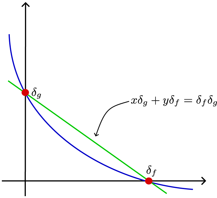
Proof. Since the Manhattan curve
 $\mathcal {C}(\mathbf {f})$
is convex and analytic, the point
 $(a,b)\in \mathcal {C}(\mathbf {f})$
is below or on the secant passing through the points
 $(\delta _f,0)$
and
 $(0,\delta _g)$
. Hence,
 $$ \begin{align*} a\delta_g+b\delta_f\leq\delta_f\delta_g, \end{align*} $$
and the equality holds if and only if
 $\mathcal {C}(\mathbf {f})$
is a straight line. See Figure 1.
The Manhattan curve and the secant between its intercepts with the axes (colour online).

We obtain (3.1) by specializing at the point
 $(a_{m_*},b_{m_*})\in \mathcal {C}(\mathbf {f})$
since
 $$ \begin{align*} H_{\mathbf{f}}(m_*) & =a_{m_*}+m_*b_{m_*}\leq\frac{\delta_f\delta_g}{\delta_g}=\delta_f. \end{align*} $$
The rigidity statement follows from Theorem 2.14(3) as
 $\mathcal {C}(\mathbf {f})$
is a straight line segment if and only if
 $$ \begin{align*} S_{n}f(\underline{x})=\frac{\delta_g}{\delta_f}S_{n}g(\underline{x}) \end{align*} $$
for all
 $\underline {x}\in \mathrm {Fix}^{\textit {n}}.$
Recall that for any
 $\alpha , \beta> 0$
, the
 $(\alpha , \beta )$
-Bishop–Steger entropy of
 ${\mathbf {f}}$
is defined as
 $$ \begin{align*} h_{(\alpha, \beta)}^{\mathrm{BS}}({\textbf{f}}) := \lim_{T \to \infty} \frac{1}{T} \log \sum_{n} \frac{1}{n} \#\{ \underline{x} \in \mathrm{ Fix}^{n}\colon \alpha S_{n} f(\underline{x}) + \beta S_{n} g(\underline{x}) \leq T \}. \end{align*} $$
Theorem 1.5. Let
 $m \in \mathcal {S}(\mathbf {f})$
be an admissible slope. Then,
 $$ \begin{align*} \frac{H_{{\textbf{f}}}(m)}{\alpha + m\beta} \leq h_{(\alpha, \beta)}^{\mathrm{BS}}({\textbf{f}}), \end{align*} $$
and the equality holds if and only if m is the unique slope satisfying
 $a_{m}/b_{m} = \alpha /\beta $
.
Proof. We ease notation by writing
 $h_{\mathrm {BS}}$
for
 $h_{(\alpha , \beta )}^{\mathrm {BS}}({\mathbf {f}})$
. From [Reference Bray, Canary, Kao and Martone5, Theorem A], we know that
 $P(-h_{\mathrm {BS}}(\alpha f + \beta g)) = 0$
, which implies
 $(a_{\mathrm {BS}}, b_{\mathrm {BS}}) := (\alpha h_{\mathrm {BS}}, \beta h_{\mathrm {BS}}) \in \mathcal {C}({\mathbf {f}})$
. Observe that
 $a_{\mathrm {BS}}/b_{\mathrm {BS}} = \alpha /\beta $
and denote by
 $m_{\mathrm {BS}}$
the slope of the normal to
 $\mathcal {C}({\mathbf {f}})$
at
 $(a_{\mathrm {BS}}, b_{\mathrm {BS}})$
. We claim that for any
 $m\in \mathcal {S}(\mathbf {f})$
,
 $$ \begin{align*} \frac{a_{m} + m b_{m}}{\alpha + m\beta} \leq \frac{a_{m_{\mathrm{BS}}} + m_{\mathrm{BS}} b_{m_{\mathrm{BS}}}}{\alpha + m_{\mathrm{BS}} \beta} = h_{\mathrm{BS}}. \end{align*} $$
The last equality follows directly from the definition of
 $h_{\mathrm {BS}}$
. To prove the inequality, note that
 $\mathcal {C}({\mathbf {f}})$
can be parameterized as
 $(s, q(s))$
, where
 $q(s)$
is an analytic function, and we denote the slope of the normal to
 $\mathcal {C}({\mathbf {f}})$
at
 $(s, q(s))$
by
 $m(s)$
so that
 $q'(s) = -1/m(s)$
. Now, consider the function
 $$ \begin{align*} F(s) = \frac{s + m(s) q(s)}{\alpha + m(s) \beta} = \frac{s - q(s)/q'(s)}{\alpha -\beta / q'(s)} = \frac{s q'(s) - q(s)}{\alpha q'(s) - \beta}. \end{align*} $$
Differentiating, we get
 $$ \begin{align*} F'(s) = \frac{q"(s)(\alpha q(s) - \beta s)}{(\alpha q'(s) - \beta)^{2}}. \end{align*} $$
Since
 $\mathcal {C}({\mathbf {f}})$
is strictly convex and real analytic, we know that
 $q"(s)> 0$
. Moreover,
 $F'(0)>0$
, while
 $F'(\delta _f)<0$
, so
 $F(s)$
achieves its maximum when
 $\alpha q(s) = \beta s$
, which implies
 $s / q(s) = \alpha / \beta $
. By the strict convexity of
 $\mathcal {C}({\mathbf {f}})$
, this solution is unique, occurring at
 $(a_{\mathrm {BS}}, b_{\mathrm {BS}}) = (\alpha h_{\mathrm {BS}}, \beta h_{\mathrm {BS}})$
. This completes the proof of the claim and the theorem.
We conclude this section by establishing technical properties of
 $H_{\mathbf {f}}(m)$
, which will be useful for the estimates carried out in the next two sections.
Lemma 3.3. Let
 $f,g\colon \Sigma ^{+}\to \mathbb {R}$
be strictly positive locally Hölder continuous potentials with strong entropy gaps at infinity such that
 $\|f-g\|_\infty $
is finite. Set
 $\mathbf {f}=(f,g)$
. Then, for every
 $m\in \mathcal S(\mathbf {f})$
:
-
(1)
$H_{\mathbf {f}}(m)=m\cdot H_{(g,f)}({1}/{m})$
; -
(2)
$H_{{\mathbf {f}}}(m)=-t_{m}\mathbb {P}^{*}(\mathbf {x}_m)$
; -
(3)
$({\textbf {x}}_{m})^{\top }\cdot \nabla ^{2}\mathbb {P}^{*}({\textbf {x}}_{m})\cdot ({\textbf {x}}_{m})>0$
, where
$\mu =\mu _{-a_{m}f-b_{m}g}.$


Proof. For the first assertion, given
 $m\in \mathcal {S}(\mathbf {f})$
, consider
 $(a_{m},b_{m})\in \mathcal {C}(\mathbf {f})$
, so that
 $P(-a_{m}f-b_mg)=0$
,
 $H_{\mathbf {f}}(m)=a_{m}+b_{m}m$
, and
 $$ \begin{align*} m=\frac{\int g\, d\mu_{-a_{m}f-b_{m}g}}{\int f\, d\mu_{-a_{m}f-b_{m}g}}. \end{align*} $$
Similarly, for
 $m'\in \mathcal {S}(g,f)$
, there is
 $(b_{m'},a_{m'})\in \mathcal {C}(g,f)$
, that is,
 $P(-b_{m'}g-a_{m'}f)=0$
, and
 $$ \begin{align*} m'=\frac{\int f\, d\mu_{-a_{m'}f-b_{m'}g}}{\int g\, d\mu_{-a_{m'}f-b_{m'}g}}. \end{align*} $$
Moreover,
 $ H_{(g,f)}(m')=b_{m'}+a_{m'}m'.$
By Theorem 2.14(4), we see that
 $m\in \mathcal {S}(\mathbf {f})$
if and only if
 $1/m\in \mathcal {S}(g,f)$
, and that when
 $m'=1/m$
, we have
 $(a_{m'},b_{m'})=(b_m,a_m)$
. Thus,
 $$ \begin{align*} H_{(g,f)}\bigg(\dfrac{1}{m}\bigg)=b_m+a_{m}\frac{1}{m}=\frac{1}{m}(a_m+mb_m)=\frac{1}{m}H_{\mathbf{f}}(m). \end{align*} $$
For item (2), by Corollary 2.16(2), we know
 $\nabla \mathbb {P}(-a_{m},-b_{m})={\textbf {x}}_m$
and
 $$ \begin{align*} \mathbb{P}^{*}({\textbf{x}}_m)=-h_{-a_{m}f-b_{m}g}(\sigma). \end{align*} $$
Hence, using the fact that
 $\mu _{-a_{m}f-b_{m}g}$
is the equilibrium state of
 $-a_{m}f-b_{m}g$
, we compute
 $$\begin{align*} -t_{m}\mathbb{P}^{*}({\textbf{x}}_m) & =\dfrac{h_{-a_{m}f-b_{m}g}(\sigma)}{\int f\, d\mu_{-a_{m}f-b_{m}g}}\\ & =\dfrac{P(-a_{m}f-b_{m}g)-\int(-a_{m}f-b_{m}g)\, d\mu_{-a_{m}f-b_{m}g}}{\int f\, d\mu_{-a_{m}f-b_{m}g}}\\ & =a_{m}+b_{m}\dfrac{\int g\, d\mu_{-a_{m}f-b_{m}g}}{\int f\, d\mu_{-a_{m}f-b_{m}g}}=a_{m}+b_{m}m\\ & =H_{{\textbf{f}}}(m). \end{align*}$$
The last assertion follows from Proposition 2.11(4) as
 $\nabla \mathbb {P}^{*}({\textbf {x}}_{m})=(-a_{m},-b_{m})$
and
 $$ \begin{align*} \nabla^{2}\mathbb{P}^{*}({\textbf{x}}_{m})=(\nabla^{2}\mathbb{P}(-a_{m},-b_{m}))^{-1}= \frac{1}{\mathrm{det\nabla^{2}\mathbb{P}}}\begin{pmatrix} \mathrm{Var}(g,\mu) & \mathrm{Cov}(f,g,\mu)\\ \mathrm{Cov}(f,g,\mu) & \mathrm{Var}(f,\mu) \end{pmatrix} ^{-1} \end{align*} $$
is positive definite (as by Corollary 2.10(4),
 $\nabla ^{2}\mathbb {P}$
is positive definite).
Remark 3.4. Using the same suspension flow interpretation as in Remark 3.2, one can relate the term in Lemma 3.3(3) with the second derivative of the pressure over the suspension flow. Explicitly,
 $$ \begin{align*} \overline{\mathbb{P}}_{m}":=t_{m}^{3}\cdot({\textbf{x}}_{m})^\top\cdot\nabla^{2}\mathbb{P}^{*}({\textbf{x}}_{m})\cdot {\textbf{x}}_{m}=\bigg(\frac{d^{2}}{dz^{2}}P_{\phi^f}|_{z=-b_{m}}(z\Psi^g)\bigg). \end{align*} $$
The convenient notation
 $\overline {\mathbb {P}}_{m}"$
will be used in §6.2.
4 Preparing to count
Before presenting the setup and results, we give a brief outline of this section. The goal here is to convert the given orbital counting problem into estimates on thermodynamical quantities. In particular, Lalley’s method counts periodic orbits by reducing this problem to studying preimages of sample points in the shift space.
To start the setup of this section, we fix a topologically mixing, countable state Markov shift
 $\Sigma ^+$
with BIP and let
 $f,g\colon \Sigma ^+\to \mathbb R$
be strictly positive locally Hölder continuous potentials with strong entropy gaps at infinity such that
 $\|f-g\|_\infty $
is finite. We let
 ${\mathbf {f}=(f,g)}$
and use the notation from §§2 and 3.
For an admissible slope
 $m\in \mathcal S(\mathbf {f})$
and a precision
 $\xi>0$
, we set
 $I_{\xi ,m}^2(t)=(t,t+\xi )\times (mt,mt+\xi )$
and define
 $$ \begin{align*} M(n,t):=M(n,t;{\textbf{f}},m,\xi)=\#\{\underline{x}\in\mathrm{Fix}^{n}\colon S_{n}\mathbf{f}(\underline{x})\in I_{\xi,m}^2(t)\}, \end{align*} $$
where
 $S_n\mathbf {f}(\underline {x}):=(S_nf(\underline {x}),S_ng(\underline {x}))$
. The goal of this section is to obtain some a priori estimates on
 $M(n,t)$
by relating it to the transfer operator
 $\mathcal {L}_{-a_mf-b_mg}$
. Our strategy is similar to the one from [Reference Bray, Canary, Kao and Martone5, §5], with some key differences which we single out below.
4.1 Preimages of sample points and a priori estimates
Fix an admissible slope
 $m\in {\mathcal {S}(\mathbf {f})}$
,
 $k\in \mathbb {Z}_{>0}$
, and a non-periodic word
 $\underline {z}_{p}\in \Sigma ^+$
in each k-cylinder
 $p\in \Lambda _{k}$
. For every
 $n\in \mathbb Z_{>0}$
and
 $\xi>0$
, define
 $$ \begin{align*} &{\mathcal{W}}(n,p,t;\mathbf{f},m,\xi)=p\cap\sigma^{-n}(\underline{z}_{p})\cap\{\underline{x}\in\Sigma^+\colon S_{n}\mathbf{f}(\underline{x})\in I^2_{\xi,m}(t)\}\quad\text{and} \\ &\quad W(n,p,t)=W(n,p,t;\mathbf{f},m,\xi):=\#\mathcal{W}(n,p,t;\mathbf{f},m,\xi). \end{align*} $$
Propositions 4.1 and 4.6 relate
 $M(n,t)$
to
 $W(n,p,t)$
, which is advantageous because
 $W(n,p,t)$
is itself related to the transfer operator via the Laplace–Fourier transform (defined below).
First, we introduce the following convenient notation. For any
 $\mathbf {y}\in \mathbb R^2$
, define
 $$ \begin{align*} M(n,\mathbf{y}):=M(n,{\textbf{y}};\mathbf{f})=\sum_{\underline{x}\in\mathrm{Fix}^{n}}{\mathbf{1}_{\{\underline{x}\colon S_{n}\mathbf{f}(\underline{x})=\mathbf{y}\}}(\underline{x})} \end{align*} $$
and for any open bounded rectangle
 $U\subset \mathbb R^2$
, let
 $$ \begin{align*} M(n,U)=\#\{\underline{x}\in\mathrm{Fix}^{n}\colon S_{n}\mathbf{f}(\underline{x})\in U\} =\int_{U}M(n,\mathbf{y})\, d\mathbf{y}. \end{align*} $$
Note that with this notation,
 $M(n,t)=M(n,I^2_{\xi ,m}(t))$
. Define
 $W(n,p,\mathbf {y})$
and
 $W(n,p,U)$
analogously and let
 $$ \begin{align*} W(n,U)=\sum_{p\in\Lambda_{k}}W(n,p,U). \end{align*} $$
Finally, for any open rectangle
 $U=(a,b)\times (c,d)$
and sufficiently small
 $\epsilon>0$
, consider the open rectangles
 $$ \begin{align*} U_{\pm\epsilon}:=(a\mp\epsilon,b\pm\epsilon)\times(c\mp\epsilon,d\pm\epsilon). \end{align*} $$
Proposition 4.1. [Reference Bray, Canary, Kao and Martone5, Lemma 5.1(ii)–(iv)]
Suppose that
 $\Sigma ^{+}$
is a topologically mixing, countable state Markov shift with BIP, then
 $f,g\colon \Sigma ^{+}\to \mathbb {R}$
are strictly positive locally Hölder continuous potentials with strong entropy gaps at infinity such that
 $\|f-g\|_\infty $
is finite.
-
(1) For any
$p\in \Lambda _{k}$
and
$n\geq k$
, there exists a bijection
$\Psi _{p}^{n}\colon \mathrm {Fix}^{n}\cap p\to \sigma ^{-n}(\underline {z}_{p})\cap p.$
-
(2) There exists a sequence
$(\epsilon _{k})_{k=1}^{\infty }$
such that
$\lim _{k}\epsilon _{k}=0$
and if
$\underline {y}\in \mathrm {Fix}^{n}\cap p$
and
$n\geq k$
, then
$$ \begin{align*} \|S_{n}\mathbf{f}(\underline{y})-S_{n}\mathbf{f}(\Psi_{p}^{n}(\underline{y}))\|\leq\epsilon_{k}. \end{align*} $$
-
(3) For all
$n\geq k$
and all open rectangles
$U\subset \mathbb {R}^{2}$
, (4.1)
$$ \begin{align} W(n,U_{-\epsilon_{k}})\leq M(n,U)\leq W(n,U_{\epsilon_{k}}). \end{align} $$


Proof. Item (1) is [Reference Bray, Canary, Kao and Martone5, Lemma 5.1(ii)], item (2) is an immediate consequence of [Reference Bray, Canary, Kao and Martone5, Lemma 5.1(iii)], and item (3) follows from item (2).
We will need to complement the results in Proposition 4.1 with an exponential control of the quantities
 $\sum _{p\in \Lambda _{k}}W(n,p,t)$
and
 $M(n,t)$
for
 $k\in \mathbb {Z}_{>0}$
and
 $n<k$
, similar to [Reference Bray, Canary, Kao and Martone5, Lemma 5.1(iv)]. However, in the current setting, we will need a different approach which relies on Lemmas 4.2 and 4.4.
Lemma 4.2. Let
 $f,g\colon \Sigma ^{+}\to \mathbb {R}$
be strictly positive locally Hölder continuous potentials with strong entropy gaps at infinity such that
 $\|f-g\|_\infty $
is finite. If
 $m\geq 1$
is an admissible slope, then
 $$ \begin{align*} d(f)<H_{\mathbf{f}}(m). \end{align*} $$
Remark 4.3. There exist potentials f and g for which every admissible slope is strictly less than 1.
Proof. By [Reference Bray, Canary, Kao and Martone5, Lemma 3.3], it suffices to show that
 $P(-H_{\mathbf {f}}(m)f)<\infty $
. Recall that, by definition, there exists a point
 $(a_{m},b_{m})$
on the Manhattan curve
 $\mathcal {C}(\mathbf {f})$
such that
 $H_{\mathbf {f}}(m)=a_{m}+m\cdot b_{m}$
. Since
 $m\geq 1$
and the pressure function is increasing by Corollary 2.10(2), we see that
 $$ \begin{align*} P(-H_{\mathbf{f}}(m)f)=P(-a_{m}f-m\cdot b_{m}f)\leq P(-a_{m}f-b_{m}f). \end{align*} $$
Then, since
 $\|f-g\|_\infty =C<\infty $
, and P is increasing and linear on constants, we see that
 $$ \begin{align*} P(-a_{m}f-b_{m}f)\leq P(-a_{m}f-b_{m}g+b_{m}C){\kern-1pt}={\kern-1pt}P(-a_{m}f-b_{m}g)+b_{m}C=b_{m}C{\kern-1pt}<{\kern-1pt}\infty, \end{align*} $$
where we used the fact that
 $P(-a_{m}f-b_{m}g)=0$
in the last equality.
Lemma 4.4. Let
 $f,g\colon \Sigma ^{+}\to \mathbb {R}$
be strictly positive locally Hölder continuous potentials with strong entropy gaps at infinity such that
 $\|f-g\|_\infty $
is finite. Suppose
 $m\geq 1$
. Then, for all
 $k\in \mathbb {N}$
and
 $b\in (d(f),H_{\mathbf {f}}(m))$
, there exists
 $C=C(k,b,\xi )>0$
such that for all
 $n<k$
and
 $t>0$
, we have
 $$ \begin{align*} \sum_{p\in\Lambda_{k}}W(n,p,t)\leq Ce^{bt} \quad\text{and}\quad M(k,t)\leq Ce^{bt}. \end{align*} $$
Remark 4.5. In this proof, we will use [Reference Bray, Canary, Kao and Martone5, Lemma 5.1(iv)]. In that result, one is only interested in the case
 $b<\delta _{f}$
. However, its proof holds more generally for any
 $b>d(f)$
(see also [Reference Bray, Canary, Kao and Martone5, Lemma 3.1]).
Proof. We notice that, by [Reference Bray, Canary, Kao and Martone5, Lemma 5.1(iv)], for all
 $b>d(f)$
, there exists
 $C=C(k,b,\xi )$
such that
 $$\begin{align*} \sum_{p\in\Lambda_{k}}W(n,p,t) & \leq\sum_{p\in\Lambda_{k}}\sum_{\underline{y}\in\sigma^{-n}(\underline{z}_{p})}\mathbf{1}_{p}(\underline{y})\mathbf{1}_{\{S_{n}f(\underline{y})\leq t+\xi\}}(\underline{y})\leq Ce^{bt}. \end{align*}$$
As
 $m\geq 1$
, we have that
 $H_{\mathbf {f}}(m)>d(f)$
by Lemma 4.2, and hence, we may choose any
 $b\in (d(f),H_{\mathbf {f}}(m)).$
The same argument shows that for all
 $b\in (d(f),H_{\mathbf {f}}(m))$
, there exists
 $C=C(k,b,\xi )$
such that
 $$ \begin{align*} \text{ }M(k,t)\leq Ce^{bt}.\\[-38pt] \end{align*} $$
We are now ready to bound
 $\sum _{p\in \Lambda _{k}}W(n,p,t)$
and
 $M(k,t)$
for any
 $k\in \mathbb {Z}_{>0}$
and
 $n<k$
.
Proposition 4.6. (Negligible parts)
Let
 $f,g\colon \Sigma ^{+}\to \mathbb {R}$
be strictly positive locally Hölder continuous potentials with strong entropy gaps at infinity such that
 $\|f-g\|_\infty $
is finite. Then, for any
 $k>0$
, there exist constants
 $\zeta =\zeta (m), C=C(k,m,\xi )>0$
such that for all
 $n<k$
,
 $$ \begin{align*} \sum_{p\in\Lambda_{k}}W(n,p,t)\leq Ce^{(H_{\mathbf{f}}(m)-\zeta)t} \quad\text{and}\quad M(k,t)\leq Ce^{(H_{\mathbf{f}}(m)-\zeta)t}. \end{align*} $$
Proof. For
 $m\geq 1$
, a stronger version is given by Lemma 4.4. Thus, we assume
 $m<1$
and consider
 $H_{(g,f)}(m')$
with
 $m'=1/m>1$
. Applying Lemma 4.4 to the pair
 $(g,f)$
, if we pick
 $\zeta $
small enough such that
 $H_{(g,f)}(m')-m'\zeta \in (d(g),H_{(g,f)}(m'))$
, then we know that there exists
 $C=C(k,m,\xi )$
such that
 $$ \begin{align*} & \sum_{p\in\Lambda_{k}}W(n,p,\widetilde{t};(g,f),m',\xi)\\ &\quad =\#(p\cap\sigma^{-n}(\underline{z}_{p})\cap\{\underline{x}\colon\ S_{n}(g,f)(\underline{x})\in I_{\xi,m'}^{2}(\widetilde{t})\})\leq Ce^{(H_{(g,f)}(m')-m'\zeta)\widetilde{t}} \end{align*} $$
for all
 $n<k$
and
 $\widetilde {t}\geq 0$
. Therefore, setting
 $\widetilde {t}=mt$
, we have
 $$ \begin{align*} \sum_{p\in\Lambda_{k}}W(n,p,t;\mathbf{f},m,\xi) & =\#(p\cap\sigma^{-n}(\underline{z}_{p})\cap\{\underline{x}\colon S_{n}\mathbf{f}(\underline{x})\in I^2_{\xi,m}(t)\})\\ & =\sum_{p\in\Lambda_{k}}W\bigg(n,p,mt;(g,f),\frac{1}{m},\xi\bigg)\\ & \leq Ce^{(H_{(g,f)}({1}/{m})-({1}/{m})\zeta)mt}\\ & =Ce^{(mH_{(g,f)}({1}/{m})-\zeta)t}\\ & =Ce^{(H_{\mathbf{f}}(m)-\zeta)t}, \end{align*} $$
where the last equality follows from Lemma 3.3(1). Applying the same argument to
 $M(k,t)$
, we obtain
 $$ \begin{align*} M(k,t)\leq Ce^{(H_{\mathbf{f}}(m)-\zeta)t}, \end{align*} $$
which ends the proof.
The Laplace–Fourier transform of a continuous function
 $F\colon \mathbb {R}^{2}\to \mathbb {R}$
is
 $$ \begin{align} \widehat{F}(\mathbf{z})=\int_{\mathbb{R}^{2}}e^{\langle{\mathbf{z},\mathbf{x}}\rangle}F(\mathbf{x})\, d{\textbf{x}}. \end{align} $$
Write
 $\widehat {W}(n,p,\mathbf {z})$
,
 $\widehat {W}(n,\mathbf {z})$
, and
 $\widehat {M}(n,\mathbf {z})$
for the Laplace–Fourier transforms of the functions
 $\mathbf {x}\mapsto W(n,p,\mathbf {x})$
,
 $\mathbf {x}\mapsto W(n,\mathbf {x})$
,
 $\mathbf {x}\mapsto M(n,\mathbf {x})$
, respectively. The key observation is that
 $\widehat {W}(n,p,\mathbf {z})$
is related to the transfer operator as follows:
 $$ \begin{align} \widehat{W}(n,p,\mathbf{z}) & =\int_{\mathbb{R}^{2}}e^{\langle\mathbf{z},\mathbf{x}\rangle}\ W(n,p,\mathbf{x})\, d{\textbf{x}}\nonumber \\ & =\int_{\mathbb{R}^{2}}e^{\langle\mathbf{z},\mathbf{x}\rangle}\sum_{\underline{y}\in\sigma^{-n}(\underline{z}_{p})}{\mathbf{1}}_{p}(\underline{y}){\mathbf{1}}_{\{\underline{y}\colon S_{n}\mathbf{f}(\underline{y})=\mathbf{x}\}}(\underline{y})\, d\mathbf{x}\nonumber \\ & =\sum_{\underline{y}\in\sigma^{-n}(\underline{z}_{p})}e^{\langle\mathbf{z},S_{n}\mathbf{f}(\underline{y})\rangle}{\mathbf{1}}_{p}(\underline{y})\nonumber\\ & =(\mathcal{L}_{\langle\mathbf{z},\mathbf{f}\rangle}^{n} {\mathbf{1}}_{p})(\underline{z}_{p}). \end{align} $$
Assume
 $\mathbf {z}\in D(\mathbf {f})$
so that
 $\langle \mathbf {z},\mathbf {f}\rangle $
is a locally Hölder continuous potential with finite pressure. By Proposition 2.5(1),
 $\mu _{\langle \mathbf {z},\mathbf {f}\rangle }$
is the unique invariant Gibbs measure and equilibrium state for
 $\langle \mathbf {z},\mathbf {f}\rangle $
, and we denote by
 $Q>1$
its Gibbs constant.
Lemma 4.7. Consider
 $k\in \mathbb N$
and
 $\mathbf {z}\in D(\mathbf {f})$
. For all
 $n\geq k,$
and
 $p\in \Lambda _{k}$
, we have that
 $$ \begin{align*} \widehat{W}(n,p,\mathbf{z})\leq Q\mu_{\langle\mathbf{z},\mathbf{f}\rangle}(p)e^{n\mathbb{P}(\mathbf{z})}, \end{align*} $$
where
 $\mu _{\langle \mathbf {z},\mathbf {f}\rangle }$
is the equilibrium state for
 $\langle \mathbf {z},\mathbf {f}\rangle $
with Gibbs constant Q.
Proof. Notice that
 $$ \begin{align*} e^{-n\mathbb{P}(\mathbf{z})}\cdot\widehat{W}(n,p,\mathbf{z})=e^{-n\mathbb{P}(\mathbf{z})}(\mathcal{L}_{\langle\mathbf{z},\mathbf{f}\rangle}^{n}{\mathbf{1}}_{p})(\underline{z}_{p}) & =\sum_{\underline{y}\in\sigma^{-n}(\underline{z}_{p})}e^{\langle\mathbf{z},S_{n}\mathbf{f}(\underline{y})\rangle-n\mathbb{P}(\mathbf{z})}{\mathbf{1}}_{p}(\underline{y})\\ & =\sum_{\underline{y}\in\sigma^{-n}(\underline{z}_{p})\cap p}e^{\langle\mathbf{z},S_{n}\mathbf{f}(\underline{y})\rangle-n\mathbb{P}(\mathbf{z})}. \end{align*} $$
Since
 $n\geq k$
, we have
 $\sigma ^{-n}(\underline {z}_{p})\cap p\neq \emptyset $
. Then, for any
 $\underline {y}\in \sigma ^{-n}(\underline {z}_{p})\cap p$
, there exists an n-cylinder
 $p_{\underline {y}}$
such that
 $\underline {y}\in p_{\underline {y}}\subset p$
. Moreover,
 $p_{\underline {y}_1}=p_{\underline {y}_2}$
implies
 $\underline {y}_1=\underline {y}_2$
. Thus, we can repeatedly use the Gibbs property to see that
 $$ \begin{align*} \sum_{\underline{y}\in\sigma^{-n}(\underline{z}_{p})\cap p}e^{\langle\mathbf{z},S_{n}\mathbf{f}(\underline{y})\rangle-n\mathbb{P}(\mathbf{z})}\leq Q\sum_{\underline{y}\in\sigma^{-n}(\underline{z}_{p})\cap p}\mu_{\langle\mathbf{z},\mathbf{f}\rangle}(p_{\underline{y}})\leq Q\mu_{\langle\mathbf{z},\mathbf{f}\rangle}(p), \end{align*} $$
which concludes the proof.
Finally, we apply Lemma 4.7 to estimate the quantity
 $$ \begin{align*} W(n,U):=\sum_{p\in\Lambda_{k}}W(n,p,U). \end{align*} $$
Lemma 4.8. Assume
 $\mathbf {z}\in D(\mathbf {f})$
, U is an open bounded rectangle in
 $\mathbb R^2$
, and
 $n\geq k$
. Let
 $\mathbf {x}\in \mathbb R^2$
be such that
 $\langle \mathbf {z},\mathbf {y}\rangle \geq \langle \mathbf {z},\mathbf {x}\rangle $
for all
 $\mathbf {y}\in U$
. Then,
 $$ \begin{align*} W(n,U)\leq Qe^{n\mathbb{P}(\mathbf{z})-\langle\mathbf{z},\mathbf{x}\rangle}. \end{align*} $$
Proof. The statement follows from the proof of [Reference Lalley25, Proposition 1]. Indeed,
 $$ \begin{align*} W(n,U) &\leq\sum_{p\in\Lambda_{k}}\int_{U}e^{\langle\mathbf{z},\mathbf{y}\rangle-\langle\mathbf{z},\mathbf{x}\rangle}W(n,p,\mathbf{y}) \,d\textbf{y} \\&\leq\sum_{p\in\Lambda_{k}}e^{-\langle\mathbf{z},\mathbf{x}\rangle}\int_{\mathbb{R}^{2}}e^{\langle\mathbf{z},\mathbf{y}\rangle}W(n,p,\mathbf{y}) \,d\textbf{y} \\ & \leq\sum_{p\in\Lambda_{k}}\widehat{W}(n,p,\mathbf{z})e^{-\langle\mathbf{z},\mathbf{x}\rangle}\leq Qe^{n\mathbb{P}(\mathbf{z})-\langle\mathbf{z},\mathbf{x}\rangle}, \end{align*} $$
where we apply Lemma 4.7 to obtain the last inequality.
5 The global growth rate control
The first goal of this section is to establish Proposition 5.1, that is, we find an a priori upper bound on the number of preimages of a fixed non-periodic word
 $\underline {z}_p$
in a cylinder p for which the nth ergodic sum of
 $\mathbf {f}$
is comparable to
 $t(1,m)$
. It is important for our purposes that these upper bounds are global, in the sense that they do not depend on p. The second goal is to establish Lemma 5.3, which is a type of large-deviation estimate. There, we single out a set of preimages of the
 $\underline {z}_p$
whose growth is relatively slow and thus negligible.
To begin the setup of this section, we fix a topologically mixing, countable state Markov shift
 $\Sigma ^+$
with BIP and strictly positive locally Hölder continuous potentials
 ${f,g\colon \Sigma ^+\to \mathbb R}$
with strong entropy gaps at infinity such that
 $\|f-g\|_\infty $
is finite. Set
 $\mathbf {f}=(f,g)$
and fix
 $\xi>0$
. Recall that for an admissible slope
 $m\in \mathcal S(\mathbf {f})$
in Notation 2.15, we defined the quantities
 $(a_m,b_m)=-\mathbf {z}_m$
,
 $t_m$
,
 $\textbf {m}$
,
 $\mathbf {x}_m={\textbf {m}}/t_m$
, and that we define the correlation number as
 $H_{\mathbf {f}}(m)=a_m+b_mm$
. Fix
 $k\in \mathbb N$
, and for each k-cylinder
 $p\in \Lambda _k$
, choose a non-periodic word
 $\underline {z}_{p}\in p$
.
In this section, we obtain growth rate estimates which are independent on the choice of a cylinder.
Proposition 5.1. (A priori estimate)
For any admissible slope
 $m\in \mathcal S(\mathbf {f})$
, there exists a constant
 $C=C(k,m,\xi )$
such that for all
 $p\in \Lambda _{k}$
, we have
 $$ \begin{align*} { \sum_{n\geq1}\sum_{\underline{y}\in\sigma^{-n}(\underline{z}_{p})}\mathbf{1}_{p}(\underline{y})\mathbf{1}_{\{t\leq S_{n}f(\underline{y})\leq t+\xi\}}(\underline{y})\mathbf{1}_{\{mt\leq S_{n}g(\underline{y})\leq mt+\xi\}}(\underline{y})\leq Ce^{tH_{{{\textbf{f}}}}(m)}\mu_{-a_{m}f-b_{m}g}(p)}, \end{align*} $$
where
 $\mu _{-a_{m}f-b_{m}g}$
is the equilibrium state for
 $-a_{m}f-b_{m}g$
.
Proposition 5.1 follows from Lemma 5.2, which is a similar a priori estimate for one potential.
Lemma 5.2. (Technical lemma)
Suppose
 $f\colon \Sigma ^+\to \mathbb R$
is a strictly positive locally Hölder continuous potential with a strong entropy gap at infinity. Let
 $\delta _f>d(f)$
be the unique constant such that
 $P(-\delta _ff)=0$
. Then, there exists a constant
 $D>0$
such that for all
 $p\in \Lambda _{k}$
,
 $$ \begin{align} \sum_{n\geq1}\sum_{\underline{y}\in\sigma^{-n}(\underline{z}_{p})}{\mathbf{1}}_{p}(y){\mathbf{1}}_{\{S_{n}f(\underline{y})\le t\}}(\underline{y})\le De^{t\delta}\mu_{-\delta f}(p), \end{align} $$
where
 $\mu _{-\delta f}$
is the equilibrium state of
 $-\delta f$
.
Proof. By [Reference Bray, Canary, Kao and Martone5, Lemma 5.1(iv)], it is enough to consider
 $n>k$
. Notice that by the Gibbs property of
 $\mu _{-\delta f}$
, we know that
 $$\begin{align*} & \sum_{n>k}\sum_{\underline{y}\in\sigma^{-n}(\underline{z}_{p})}{\mathbf{1}}_{p}(\underline{y}){\mathbf{1}}_{\{S_{n}f(\underline{y})\le t\}}(\underline{y}) \\ &\quad =\sum_{n>k}\sum_{\underline{y}\in\sigma^{-n}(\underline{z}_{p})}{\mathbf{1}}_{p}(\underline{y}){\mathbf{1}}_{\{S_{n-k}f(\sigma^{k}(\underline{y}))\le t-S_{k}f(\underline{y})\}}(\underline{y})\\ &\quad \leq\sum_{n>k}\sum_{\underline{y}\in\sigma^{-n}(\underline{z}_{p})}{\mathbf{1}}_{p}(\underline{y}){\mathbf{1}}_{\bigg\{S_{n-k}f(\sigma^{k}(\underline{y}))\le t+\dfrac{\log\mu_{-\delta f}(p)+\log Q}{\delta}\bigg\}}(\underline{y})\\ & \quad \leq\sum_{n>k}\sum_{\underline{w}\in\sigma^{k-n}(\underline{z}_{p})}{\mathbf{1}}_{\bigg\{S_{n-k}f(\underline{w})\le t+\dfrac{\log\mu_{-\delta f}(p)+\log Q}{\delta}\bigg\}}(\underline{w})\\ & \quad =\sum_{m\geq1}\sum_{\underline{w}\in\sigma^{-m}(\underline{z}_{p})}{\mathbf{1}}_{\bigg\{S_{m}f(\underline{w})\le t+\dfrac{\log\mu_{-\delta f}(p)+\log Q}{\delta}\bigg\}}(\underline{w})\\ & \quad \leq \widetilde Ce^{\delta\bigg(t+\dfrac{\log\mu_{-\delta f}(p)+\log Q}{\delta}\bigg)}=\widetilde CQe^{\delta t}\mu_{-\delta f}(p), \end{align*}$$
where Q is the Gibbs constant of
 $\mu _{-\delta _f}$
and the last inequality follows from [Reference Bray, Canary, Kao and Martone5, Lemma 4.3].
Proof of Proposition 5.1
Let us simplify notation by writing
 $a=a_{m}$
,
 $b=b_{m}$
,
 $H=H_{{\textbf {f}}}(m)=a+bm$
, and
 $\mu =\mu _{-af-bg}$
. We first claim that there exists E such that
 $$ \begin{align*} { \sum_{n\geq1}\sum_{\underline{y}\in\sigma^{-n}(\underline{z}_{p})}\mathbf{1}_{p}(\underline{y})\mathbf{1}_{\{S_{n}f(\underline{y})\leq t\}}(\underline{y})\mathbf{1}_{\{|S_{n}(g-mf)(\underline{y})|\leq\xi\}}(\underline{y})\leq Ce^{tH}\mu(p)}. \end{align*} $$
Let
 $\varphi =({1}/{H})(af+bg)$
and observe that
 $\varphi $
is a strictly positive locally Hölder continuous potential satisfying
 $P(-H\varphi )=0$
. Using Lemma 5.2, we know that there exists a constant
 $D>0$
such that for all
 $p\in \Lambda _{k}$
,
 $$ \begin{align} { \sum_{n\geq1}\sum_{\underline{y}\in\sigma^{-n}(\underline{z}_{p})}\mathbf{1}_{p}(\underline{y})\mathbf{1}_{\{S_{n}\varphi(\underline{y})\leq t\}}(\underline{y})\leq De^{tH}\mu(p)}, \end{align} $$
where we note that
 $\mu $
is the equilibrium state for
 $-H\varphi =-af-bg$
. Since
 $a=H-bm$
, we have
 $$ \begin{align*} \varphi=\frac{1}{H}(af+bg)=f+\frac{b}{H}(g-mf). \end{align*} $$
Hence, we know that for any n and
 $\underline {y}\in \Sigma ^{+}$
,
 $$ \begin{align} &\mathbf{1}_{\{S_{n}f(\underline{y})\leq t\}}(\underline{y})\mathbf{1}_{\{|S_{n}(g-mf)(\underline{y})|\leq\xi\}}(\underline{y}) \nonumber\\ & \quad\leq \mathbf{1}_{\{S_{n}f(\underline{y})+({b}/{H})S_{n}(g-mf)(\underline{y})\leq t+({b}/{H})\xi\}}(\underline{y})=\mathbf{1}_{\{S_{n}\varphi(\underline{y})\leq t+({b}/{H})\xi\}}(\underline{y}). \end{align} $$
By (5.2) and (5.3), we finally obtain
 $$ \begin{align*} & \sum_{n\geq1}\sum_{\underline{y}\in\sigma^{-n}(\underline{z}_{p})}\mathbf{1}_{p}(\underline{y})\mathbf{1}_{\{S_{n}f(\underline{y})\leq t\}}(\underline{y})\mathbf{1}_{\{|S_{n}(g-mf)(\underline{y})|\leq\xi\}}(\underline{y})\\ & \quad \leq De^{({b\xi}/{H})}e^{tH}\mu(p)=:Ee^{tH}\mu(p), \end{align*} $$
which completes the proof of the claim. Then, we get
 $$\begin{align*} &\sum_{n\geq1}\sum_{\underline{y}\in\sigma^{-n}(\underline{z}_p)}\mathbf{1}_{p}(\underline{y})\mathbf{1}_{\{t\leq S_{n}f(\underline{y})\leq t+\xi\}}(\underline{y})\mathbf{1}_{\{mt\leq S_{n}g(\underline{y})\leq mt+\xi\}}(\underline{y})\\ &\quad \leq \sum_{n\geq1}\sum_{\underline{y}\in\sigma^{-n}(\underline{z}_p)}\mathbf{1}_{p}(\underline{y})\mathbf{1}_{\{t\leq S_{n}f(\underline{y})\leq t+\xi\}}(\underline{y})\mathbf{1}_{\{|S_{n}g(\underline{y})-mS_{n}f(\underline{y})|\leq(m+1)\xi\}}(\underline{y})\\ &\quad \leq \sum_{n\geq1}\sum_{\underline{y}\in\sigma^{-n}(\underline{z}_p)}\mathbf{1}_{p}(\underline{y})\mathbf{1}_{\{S_{n}f(\underline{y})\leq t+\xi\}}(\underline{y})\mathbf{1}_{\{|S_{n}g(\underline{y})-mS_{n}f(\underline{y})|\leq(m+1)\xi\}}(\underline{y})\\ &\quad \leq \underset{C}{\underbrace{De^{\bigg(\dfrac{b(m+1)\xi}{H}+H\xi\bigg)}}}e^{tH}\mu(p), \end{align*}$$
which finishes the proof of the proposition.
Recall the notation
 $I_{\xi ,m}^{2}(t)=(t,t+\xi )\times (mt,mt+\xi )$
and consider the set
 $$ \begin{align*} \mathcal{W}(p,t):=\{\underline{y}\in\Sigma^{+}\colon\underline{y}\in p,\ \sigma^{n}(\underline{y})=\underline{z}_{p},\ S_{n}\mathbf{f}(\underline{y})\in I_{\xi,m}^{2}(t) \text{ for some }{n\geq1}\}. \end{align*} $$
Since we assume that
 $\underline {z}_p$
is not periodic, if
 $\underline {y}\in \mathcal W(p,t)$
, then there exists a unique positive integer
 $n(\underline {y})$
such that
 $\sigma ^{n(\underline {y})}(\underline {y})=\underline {z}_{p}$
. Now, for any
 $\epsilon>0$
, define
 $$ \begin{align*} & \mathcal{W}(p,t,\geq\epsilon):=\bigg\{ \underline{y}\in\mathcal{W}(p,t)\colon\bigg|\frac{n(\underline{y})}{t}-t_{m}\bigg|\geq\epsilon\bigg\} \quad\text{ and }\quad\\ & \mathcal{W}(p,t,<\epsilon):=\bigg\{ \underline{y}\in\mathcal{W}(p,t)\colon\bigg|\frac{n(\underline{y})}{t}-t_{m}\bigg|<\epsilon\bigg\}. \end{align*} $$
Observe that these sets are related to the quantities
 $W(n,p,t)$
introduced in §4 and, in particular,
 $$ \begin{align*} \#\mathcal W(p,t)=\sum_{n\geq 1}W(n,p,t). \end{align*} $$
We now derive a type of large deviation result which shows that the contribution to the growth of
 $\mathcal {W}(p,t)$
by the elements
 $\underline {y}$
for which
 $n(\underline {y})/t$
is far from
 $t_m$
is negligible.
Lemma 5.3. (Negligible part)
Suppose
 $m\in \mathcal S(\mathbf {f})$
is an admissible slope for
 $\mathbf {f}$
. For any
 $\epsilon>0$
, there exist constants
 $C_{2}=C_2(k,m,\xi ,\epsilon ),\eta =\eta (k,m,\xi ,\epsilon )>0$
such that
 $$ \begin{align*} \sum_{p\in\Lambda_{k}}\mathcal{W}(p,t,\geq\epsilon)=\sum_{p\in\Lambda_{k}}{ \sum_{n\colon|({n}/{t})-t_{m}|\geq\epsilon}W(n,p,t)\leq C_{2}e^{t(H_{\mathbf{f}}(m)-\eta)}}. \end{align*} $$
Proof. When
 $n<k$
, the statement follows from a repeated application of Proposition 4.6. Thus, assume
 $n\geq k$
and let
 ${\textbf {m}}=(1,m)$
. By Lemma 2.12(2), we know that the function
 $t\mapsto -t\mathbb {P}^{*}({\textbf {m}}/{t})$
is concave down and realizes its maximum at
 $t=t_{m}$
. Let
 $t^{1}=t_{m}+\epsilon $
,
 $t^{0}=t_{m}-\epsilon $
, and
 $\mathbf {z}^{i}=\nabla \mathbb {P^{*}}({\mathbf {m}}/{t^{i}})$
for
 $i=0,1$
. By Proposition 2.11(4), we have
 $$ \begin{align*} \mathbb{P}(\mathbf{z}^{1})<0=\mathbb P\bigg(\nabla\mathbb{P}^{*}\bigg(\frac{\mathbf{m}}{t_m}\bigg)\bigg)<\mathbb{P}(\mathbf{z}^{0}) \end{align*} $$
and
 $t^{i}\mathbb {P}(\mathbf {z}^{i})-\langle \mathbf {m},\mathbf {z}^{i}\rangle <H_{\mathbf {f}}(m)$
by Proposition 2.11(6) and Lemma 3.3(2).
Consider
 $U_{t}=(1,1+({\xi }/{t}))\times (m,m+({\xi }/{t}))$
, so that
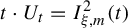 $t\cdot U_{t}=I_{\xi ,m}^{2}(t)$
. Recall that Lemma 4.8 shows that for all
 $n\ge k$
and for a fixed
 $\mathbf {z}\in D$
, if
 $\mathbf {x}\in \mathbb {R}^{2}$
is such that
 $\langle \mathbf {z},\mathbf {y}\rangle \geq \langle \mathbf {z},\mathbf {x}\rangle $
for all
 $\mathbf {y}\in U_{t}$
, then
 $$ \begin{align*} W(n,U_{t})\leq Qe^{n\mathbb{P}(\mathbf{z})-\langle\mathbf{z},\mathbf{x}\rangle}. \end{align*} $$
Notice that the linear functional
 $\mathbf {y}\mapsto \langle \mathbf {z},\mathbf {y}\rangle $
for
 $\mathbf {y}\in \overline {U}_{t}$
reaches its extreme values at a vertex of
 $\overline {U}_{t}$
.
We let
 $\mathbf {x}^{i}(t)$
be the vertex of
 $\overline {U}_{t}$
such that
 $\langle \mathbf {z}^{i},\mathbf {y}\rangle \geq \langle \mathbf {z}^{i},\mathbf {x}^{i}(t)\rangle $
for all
 $\mathbf {y}\in U_{t}$
. We also notice that
 $|\mathbf {x}^{i}(t)-\mathbf {m}|\leq \sqrt {2}({\xi }/{t})$
. With this notation, we have
 $$ \begin{align*} W(n,I_{\xi,m}^{2}(t)) & \leq Qe^{n\mathbb{P}(\mathbf{z}^{1})-t\langle\mathbf{z}^{1},\mathbf{x}^{1}(t)\rangle} \end{align*} $$
and given that
 $\mathbb {P}(\mathbf {z}^{1})<0$
, we obtain
 $$ \begin{align*} \sum_{n\geq tt^{1}}W(n,I_{\xi,m}^{2}(t)) & \leq\sum_{n\geq tt_{1}}Qe^{n\mathbb{P}(\mathbf{z}^{1})-t\langle\mathbf{z}^{1},\mathbf{x}^{1}(t)\rangle}\ \ \\ & \leq Q\cdot\frac{e^{tt^{1}\mathbb{P}(\mathbf{z}^{1})-t\langle\mathbf{z}^{1},\mathbf{x}^{1}(t)\rangle}}{1-e^{\mathbb{P}(\mathbf{z}^{1})}} =Q'e^{t(t^{1}\mathbb{P}(\mathbf{z}^{1})-\langle\mathbf{z}^{1},\mathbf{x}^{1}(t)\rangle)}\\ & \leq \overline Q'e^{t(H_{\mathbf{f}}(m)-\eta_{1})}. \end{align*} $$
Similarly,
 $$ \begin{align*} \sum_{n\leq tt^{0}}W(n,I_{\xi,m}^{2}(t)) & \leq\sum_{n\leq tt^{0}}Qe^{n\mathbb{P}(\mathbf{z}^{0})-t\langle\mathbf{z}^{0},\mathbf{x}^{0}(t)\rangle}\\ & \leq Q\cdot\frac{e^{\mathbb{P}(\mathbf{z}^{0})}(e^{tt^{0}\mathbb{P}(\mathbf{z}^{0})}-1)e^{-t\langle\mathbf{z}^{0},\mathbf{x}^{0}(t)\rangle}}{e^{\mathbb{P}(\mathbf{z}^{0})}-1}= Q"e^{t(t^{0}\mathbb{P}(\mathbf{z}^{0})-\langle\mathbf{z}^{0},\mathbf{x}^{0}(t)\rangle)}\\ & \leq \overline Q"e^{t(H_{\mathbf{f}}(m)-\eta_{2})}.\\[-38pt] \end{align*} $$
Lemma 5.4. There exists a constant
 $C_3=C_3(k,m,\xi )>0$
independent of p such that
 $$ \begin{align*} \sum_{p\in\Lambda_{k}}\sum_{n\geq1}\frac{1}{n}W(n,p,t)\leq C_3\frac{e^{H_{\mathbf{f}}(m)t}}{t}, \end{align*} $$
where
 $W(n,p,t)=\#(p\cap \sigma ^{-n}(\underline {z}_{p})\cap \{\underline {y}\colon S_{n}\mathbf {f}(\underline {y})\in I_{\xi ,m}^{2}(t)\})$
.
Proof. This follows from Proposition 5.1 and Lemma 5.3 via the following estimate:
 $$ \begin{align*} \sum_{p\in\Lambda_{k}}\sum_{n\geq1}\frac{1}{n}W(n,p,t) & = \sum_{p\in\Lambda_{k}}\sum_{\underline{y}\in\mathcal{W}(p,t)}\frac{1}{n(\underline{y})}\\ & = \sum_{p\in\Lambda_{k}}\sum_{y\in\mathcal{W}(p,t,\geq\epsilon)}\frac{1}{n(\underline{y})} + \sum_{p\in\Lambda_{k}}\sum_{\underline{y}\in\mathcal{W}(p,t,<\epsilon)}\frac{1}{n(\underline{y})}\\ & \leq C_{2}e^{t(H_{\mathbf{f}}(m)-\eta)} + \sum_{p\in\Lambda_{k}}\sum_{\underline{y}\in\mathcal{W}(p,t,<\epsilon)}\frac{1}{t(t_{m}-\epsilon)}\\ & \leq C_{2}e^{t(H_{\mathbf{f}}(m)-\eta)} + \frac{Ce^{tH_{{{\textbf{f}}}}(m)}}{t(t_m-\epsilon)}\sum_{p\in\Lambda_{k}}\mu_{-a_mf-b_mg}(p)\\ & \leq \frac{C_{3}e^{tH_{{{\textbf{f}}}}(m)}}{t}, \end{align*} $$
where
 $C_{2}$
is the constant from Lemma 5.3, C is the constant from Proposition 5.1, and
 ${C}/{t_{m}-\varepsilon }$
is uniformly bounded for t sufficiently large (for instance, when
 $t_{m}>2\varepsilon $
). Hence, a constant
 $C_{3}$
in the last inequality exists.
6 Local counting, asymptotic estimates, and Theorems 1.1, 1.2, and 1.3
We begin by outlining the structure of this section. Our goal is to combine the global estimates derived in §5 with the local asymptotic expansion formula in Theorem 6.1 to establish the main results of the paper, namely Theorems 1.1, 1.2, and 1.3.
Let
 $\Sigma ^+$
be a topologically mixing, countable state Markov shift with BIP and let
 $f,g\colon \Sigma ^+\to \mathbb R$
be strictly positive locally Hölder continuous potentials with strong entropy gaps at infinity such that
 $\|f-g\|_\infty $
is finite. Set
 $\mathbf {f}=(f,g)$
. Fix an admissible slope
 ${m\in \mathcal S(\mathbf {f})}$
and recall Notation 2.15 for
 $(a_m,b_m)=-\mathbf {z}_m$
,
 $t_{m}$
,
 ${\textbf {m}}$
, and
 ${\textbf {x}}_{m}={\textbf {m}}/t_m$
. Furthermore, as in Theorem 2.6, we let
 $h_{-a_m f - b_m g}$
and
 $\nu _{-a_m f - b_m g}$
denote the eigenfunction and eigenmeasure of the transfer operator
 $\mathcal {L}_{-a_m f - b_m g}$
, respectively. Throughout this section, we fix
 $k\in \mathbb N$
, a k-cylinder
 $p\in \Lambda _{k}$
, and a non-periodic word
 $\underline {z}_p\in p$
.
The main goal of this section is to establish the following local estimate.
Theorem 6.1. (Local estimate)
Let
 $m\in \mathcal {S}({\mathbf {f}})$
and consider
 $(a_{m},b_{m})\in \mathcal {C}(\mathbf {f})$
. Then, as
 $t\to \infty $
,
 $$ \begin{align*} \sum_{n\geq1}\frac{1}{n}W(n,p,t)\sim\frac{e^{tH_{\mathbf{f}}(m)}}{t^{({3}/{2})}}(2\pi\overline{\mathbb{P}}^{\prime\prime}_{m})^{-({1}/{2})}\cdot C_{p}(m)\cdot \int_{0}^{\xi}e^{a_{m}t}\, dt\cdot \int_{0}^{\xi}e^{b_{m}t}\, dt, \end{align*} $$
where
 $\overline {\mathbb {P}}^{\prime \prime }_{m}:=t_{m}^{3}\cdot ({\textbf {x}}_{m})^\top \cdot \nabla ^{2}\mathbb {P}^{*}({\textbf {x}}_{m})\cdot {\textbf {x}}_{m}$
and
 $C_{p}(m)=h_{-a_{m}f-b_{m}g}(\underline {z}_{p})\nu _{-a_{m}f-b_{m}g}(p)$
.
Remark 6.2. The notation
 $\overline {\mathbb {P}}^{\prime \prime }_{m}$
is used to simplify the right-hand side in Theorem 6.1. One can also see Remark 3.4 for another interpretation of
 $\overline {\mathbb {P}}^{\prime \prime }_{m}$
as the second derivative of the pressure over the suspension flow.
6.1 The proofs of Theorems 1.1, 1.2, and 1.3
Theorem 6.1 is the last ingredient needed to establish Theorems 1.1, 1.2, and 1.3 from the introduction. In this subsection, we record the proofs of these results while assuming Theorem 6.1.
Theorem 6.3. (Theorem 1.1 and Theorem 1.3)
For any
 $m\in \mathcal {S}({\mathbf {f}})$
, we have
 $$ \begin{align*} \lim_{t\to\infty}\frac{1}{t}\log M(t;{\mathbf{f},m,\xi)}=H_{\mathbf{f}}(m). \end{align*} $$
Proof. Fix
 $k\in \mathbb N$
. For
 $n\geq k$
, we apply Proposition 4.1(3) with
 $U=I^2_{\xi ,m}(t)$
to deduce that for any
 $p\in \Lambda _k$
,
 $$ \begin{align} W(n,p,t;\mathbf{f},m,\xi-\epsilon_k)\leq \#\mathcal{M}_p(n,t;{\mathbf{f},m,\xi)}\leq W(n,p,t;\mathbf{f},m,\xi+\epsilon_k), \end{align} $$
where
 $(\epsilon _k)_k$
is the sequence from Proposition 4.1(2). Then, we apply Proposition 4.6 to see that there exists
 $\zeta =\zeta (m)>0$
and
 $C_{1}=C_1(k,m,\xi )>0$
such that for any
 $n<k$
,
 $$ \begin{align} \#\mathcal{M}(n,t;{\textbf{f}},m,\xi)\leq C_{1}e^{t(H_{\mathbf{f}}(m)-\zeta)}. \end{align} $$
Moreover, Lemma 5.4 and Theorem 6.1 show that there exists
 $C_{2}=C_2(m,p,\xi )$
and
 $C_{3}=C_3(k,m,\xi )$
such that
 $$ \begin{align*} \frac{e^{tH_{\mathbf{f}}(m)}}{t^{{3}/{2}}}(C_2+o(1))= \sum_{n\geq 1} \frac{1}{n} W(n,p,t)\leq \sum_{p\in\Lambda_k}\sum_{n\geq 1} \frac{1}{n} W(n,p,t)\leq C_{3}\frac{e^{tH_{\mathbf{f}}(m)}}{t}. \end{align*} $$
Thus, recalling that
 $M(t;\mathbf {f},m,\xi )=\sum _{p\in \Lambda _k}\sum _{n\geq 1}({1}/{n})\#\mathcal M_p(n,t;\mathbf {f},m,\xi )$
, we obtain
 $$ \begin{align*} \lim_{t\to\infty}\frac{1}{t}\log M(t;{\textbf{f},m,\xi)}=H_{\mathbf{f}}(m).\\[-42pt] \end{align*} $$
Remark 6.4. We expect the asymptotic growth rate of
 $\sum _{p\in \Lambda _k}\sum _{n\geq 1} ({1}/{n}) W(n,p,t)$
to be
 ${e^{tH_{\mathbf {f}}(m)}}/{t^{3/2}}$
, up to a constant, as suggested by Theorem 1.2. The key missing step for establishing the global version of Theorem 1.2 is to improve the current upper bound in Lemma 5.4 from
 ${e^{tH_{\mathbf {f}}(m)}}/t$
to
 ${e^{tH_{\mathbf {f}}(m)}}/{t^{3/2}}$
.
Proof of Theorem 1.2
By Theorem 6.1, we know
 $$ \begin{align*} \sum_{n\geq1}\frac{1}{n}W(n,p,t;{\textbf{f},m,\xi)=\frac{e^{tH_{\mathbf{f}}(m)}}{t^{{3}/{2}}}C(m,p,\xi)(1+o(1))}, \end{align*} $$
where
 $C(m,p,\xi )=(2\pi \overline {\mathbb {P}}^{\prime \prime }_{m})^{-1/2}\cdot C_{p}(m)\cdot \int _{0}^{\xi }e^{a_{m}t}\, dt\cdot \int _{0}^{\xi }e^{b_{m}t}\, dt.$
Moreover, by (6.1) and (6.2), we get
 $$ \begin{align*} & \frac{e^{tH_{\mathbf{f}}(m)}}{t^{{3}/{2}}}C(m,p,\xi-\epsilon_k)(1+o(1))\\ &\quad \leq\sum_{n\geq1}\frac{1}{n}\#\mathcal{M}_p(n,t;{\textbf{f},m,\xi)\leq\frac{e^{tH_{\mathbf{f}}(m)}}{t^{{3}/{2}}}C(m,p,\xi+\epsilon_k)(1+o(1))}. \end{align*} $$
To conclude the proof, recall that
 $\epsilon _k\to 0$
as
 $k\to \infty $
by Proposition 4.1(2).
6.2 Proof of Theorem 6.1
This proof consists of three steps. First, for any
 $\epsilon>0$
, we break the sum into two parts:
 $$ \begin{align*} \sum_{n\geq1}\frac{1}{n}W(n,p,t)=\sum_{n:\ |({n}/{t})-t_{m}|\ge\epsilon}\frac{1}{n}W(n,p,t)+\sum_{n:\ |({n}/{t})-t_{m}|<\epsilon}\frac{1}{n}W(n,p,t). \end{align*} $$
By Lemma 5.3, for any
 $\epsilon>0$
,
 $$ \begin{align*} \limsup_{t\to\infty}e^{-tH_{{\textbf{f}}}(m)}\cdot t^{{3}/{2}}\bigg(\sum_{n:\ |({n}/{t})-t_{m}|\geq\epsilon}\frac{1}{n}W(n,p,t)\bigg)\leq\limsup_{t\to\infty}C_{2}t^{{3}/{2}}e^{-t\eta}=0. \end{align*} $$
Therefore, for any
 $\epsilon>0$
, it suffices to study the asymptotic behavior for
 $t\to \infty $
of
 $$ \begin{align*} \sum_{n:\ |({n}/{t})-t_{m}|<\epsilon}\frac{1}{n}W(n,p,t). \end{align*} $$
Since the characteristic function of the rectangle
 $(0,\xi )\times (0,\xi )$
can be approximated by a non-negative smooth function u with compact support, it is enough to show that
 $$ \begin{align} &\lim_{\epsilon\to0}\lim_{t\to\infty}e^{-tH_{{\textbf{f}}}(m)}\, t^{{3}/{2}}\bigg(\sum_{n:\,|({n}/{t})-t_{m}|<\epsilon}\frac{1}{n} \int_{\mathbb{R}^{2}}u({\textbf{y}}-t{\textbf{m}}) W(n,p,{\textbf{y}})\, d{\textbf{y}}\bigg)\nonumber\\ &\quad =(2\pi\overline{\mathbb{P}}^{\prime\prime}_{m})^{-({1}/{2})}C_{p}(m)\int_{\mathbb{R}^{2}}u({\textbf{y}})\, e^{-\langle \mathbf{z}_{m}, {\textbf{y}} \rangle}\, d{\textbf{y}}. \end{align} $$
We will need Lemma 6.5 below, whose proof is postponed to §6.3. For
 $N\in \mathbb N$
, denote by
 $C_c^N(\mathbb R^2)$
the space of N-differentiable functions on
 $\mathbb R^2$
with compact support.
Lemma 6.5. Let K be a compact neighborhood of
 $\mathbf {x}_m$
in
 $\nabla \mathbb P(D)$
. Suppose
 ${\mathbf {x}=\nabla }\mathbb {P}({\textbf {z})}\in K$
and
 $u\in C_{c}^{N}(\mathbb {R}^{2})$
is non-negative, then as
 $n\to \infty $
,
 $$ \begin{align*} \int u({\textbf{y}-n{\textbf{x}})W(n,p,\mathbf{y})\, d \mathbf{y}\sim\frac{e^{-n\mathbb{P}^{*}({\textbf{x}})}}{2\pi n}(\det\nabla\mathbb{P}^{*}({\textbf{x}}))^{1/2}\cdot C_{p}(\mathbf{z})\cdot\int_{\mathbb{R}^{2}}u({\textbf{y})}e^{-\langle{\textbf{z}},{\textbf{y}}\rangle}\, d{\textbf{y}},} \end{align*} $$
where
 $C_{p}(\mathbf {z})=h_{\langle {\mathbf {z},\mathbf {f}}\rangle }(\underline {z}_{p})\nu _{\langle {\mathbf {z},\mathbf {f}}\rangle }(p)$
. Furthermore, the above convergence is uniform in K.
Remark 6.6. Let us outline the strategy for obtaining (6.3) assuming Lemma 6.5. The first step is to derive (6.4) below, which provides the asymptotic expansion for the left-hand side of (6.3) for points near
 ${\mathbf {x}}_{m}$
. Next, we expand the left-hand side of (6.4), denoted by
 $(*)$
, and terms such as
 $\overline {\mathbb {P}}^{\prime \prime }_{m}$
appearing in (6.3) arise naturally. Using this expansion, together with Lemma 6.7, a Gaussian-type distribution result, we can rewrite and bound the left-hand side of (6.4), that is,
 $(*)$
, in terms of
 $\overline {\mathbb {P}}^{\prime \prime }_{m}$
and the other quantities in (6.3). Equation (6.3) then follows by taking the limits of the upper and lower bounds for
 $(*)$
.
We now begin with the first step. We plan to apply Lemma 6.5 to points
 ${\mathbf {x}}$
near
 ${\mathbf {x}}_{m} = {\textbf {m}}/t_{m}$
(cf. Notation 2.15), in particular, to those of the form
 ${\mathbf {x}} = {\textbf {m}}/(n/t)$
whenever
 $|n/t - t_{m}| < \epsilon $
for small
 $\epsilon $
. To do this, we need to ensure that these points lie in
 $\nabla \mathbb {P}(D)$
. To see this, note first that D is an open set (by Proposition 2.5(3)), and that
 $\nabla \mathbb {P}$
is a homeomorphism on D. The latter follows from the inverse function theorem and because
 $\nabla ^{2}\mathbb {P}$
is positive definite (Corollary 2.10(4)). Consequently,
 $\nabla \mathbb {P}(D) \subset \mathbb {R}^{2}$
is open.
Since
 ${\mathbf {x}}_{m}$
lies in the open set
 $\nabla \mathbb {P}(D)$
, there exists
 $\epsilon> 0$
sufficiently small such that whenever
 $|n/t - t_{m}| < \epsilon $
, the point
 ${\textbf {m}}/(n/t)$
lies in a neighborhood of
 ${\mathbf {x}}_{m}$
contained in
 $\nabla \mathbb {P}(D)$
. Thus, there exists
 $ {\mathbf {z}}^{*} := \nabla \mathbb {P}^{*}\!({{\textbf {m}}}/{n/t}) \in D. $
Then, summing the estimate from Lemma 6.5 over the set
 $\{n:|{n}/{t}-t_{m}|<\epsilon \}$
, for
 $t\to \infty $
, we have
 $$ \begin{align} & \sum_{|{n}/{t}-t_{m}|<\epsilon}\frac{1}{n}\int u({\textbf{y}}-t{\textbf{m}})W(n,p,{\textbf{y}})\, d{\textbf{y}}\nonumber\\ & \quad \sim\underset{:=~(*)}{\underbrace{\sum_{|({n}/{t})-t_{m}|<\epsilon}\frac{e^{-n\mathbb{P}^{*}(t{\textbf{m}}/n)}}{2\pi n^{2}}\cdot(\det\nabla^{2}\mathbb{P}^{*}(t{\textbf{m}}/n))^{1/2}\cdot\mathbf{Q}_{p}(t{\textbf{m}/n})}}, \end{align} $$
where
 $\mathbf {Q}_{p}(t{\textbf {m}}/n)\colon =C_p(\mathbf {z}^*)\int _{\mathbb R^2} u(\mathbf {y})e^{-\langle {\mathbf {z}}^*,\mathbf {y}\rangle }$
. Now, the last step in the proof of Theorem 6.1 consists of using a standard probability trick, Lemma 6.7 below, to simplify the right-hand side of the above equation.
Lemma 6.7. (Lalley [Reference Lalley25, Lemma 6])
Suppose F is continuous on a closed interval
 $[t_{1},t_{2}]$
and
 $t_{1}<t_{m}<t_{2}$
. Let
 $\sigma>0$
. Then, for any
 $\epsilon>0$
such that
 $(t_m-\epsilon ,t_m+\epsilon )\subset [t_{1},t_{2}]$
, we have
 $$ \begin{align} \lim_{t\to\infty}\sum_{n\colon|({n}/{t})-t_m|<\epsilon}\frac{1}{t^{1/2}}F\bigg(\frac{n}{t}\bigg)e^{-({t(({n}/{t})-t_m)^{2}}/{2\sigma^{2}})}=F(t_m)(2\pi)^{1/2}\sigma. \end{align} $$
Moreover, (6.5) holds uniformly for
 $t_m$
and
 $\sigma $
in a compact subset of
 $(0,\infty )$
, and F in a compact subset of
 $C([t_{1},t_{2}])$
with
 $t_{1}<t_m<t_{2}$
.
Recall that by Lemma 2.12(2) and Corollary 2.16(4),
 $s\mapsto -s\mathbb {P^{*}}({\textbf {m}}/s)$
is concave down for
 $s>0$
and achieves its maximum uniquely at
 $s=t_{m}$
. Expanding
 $-s\mathbb {P^{*}}({\textbf {m}}/s)$
near
 $t_{m}$
, we have
 $$\begin{align*} -\frac{n}{t}\mathbb{P}^{*}\bigg({\textbf{m}}\frac{t}{n}\bigg)&= -t_{m}\mathbb{P}^{*}({\textbf{m}}/t_{m})-t_{m}^{-1}({\textbf{m}}/t_{m})^\top\cdot\nabla^{2}\mathbb{P}^{*}({\textbf{m}}/t_{m})\cdot({\textbf{m}}/t_{m})\cdot \frac{|{n}/{t}-t_{m}|^{2}}{2}\\& \qquad+R(\zeta,m)\bigg|\dfrac{n}{t}-t_{m}\bigg|^{3}\\& = \underset{H_{{\textbf{f}}}(m)}{\underbrace{-t_{m}\mathbb{P}^{*}({\mathbf{x}}_{m})}}-\underset{\text{main contribution}}{\underbrace{t_{m}^{-1}({\textbf{x}}_{m})^\top\cdot\nabla^{2}\mathbb{P}^{*}({\textbf{x}}_{m})\cdot{\textbf{x}}_{m}\cdot \frac{|{n}/{t}-t_{m}|^{2}}{2}}}+\underset{\text{negligible term}}{\underbrace{R(\zeta,m)\bigg|\dfrac{n}{t}-t_{m}\bigg|^{3}}}, \end{align*}$$
where
 $R(\zeta , m)$
is the remainder term from the Taylor expansion for some
 $\zeta \in (({n}/{t}),\, t_{m})$
. Since the function
 $s\mapsto -s\mathbb {P^{*}}({\textbf {m}}/s)$
is analytic around
 $s=t_{m}$
, there exists a constant
 $C_{m,\epsilon }>0$
such that
 $|R(\zeta ,x)|\leq C_{m,\epsilon }$
. Recalling that
 $$ \begin{align*} t_{m}^{-1}({\textbf{x}}_{m})^\top\cdot\nabla^{2}\mathbb{P}^{*}({\textbf{x}}_{m})\cdot{\textbf{x}}_{m}=t_{m}^{-4}\overline{\mathbb{P}}^{\prime\prime}_{m}, \end{align*} $$
for n such that
 $|({n}/{t})-t_{m}|<\epsilon $
, we estimate
 $$ \begin{align} (*)\leq\sum_{|({n}/{t})-t_{m}|<\epsilon}&\underset{=e^{tH_{{\textbf{f}}}(m)}\cdot e^{-({t|({n}/{t})-t_{m}|^{2}})/{2\sigma_{+}^{2}}}} {\underbrace{e^{tH_{{\textbf{f}}}(m)-tt_{m}^{-4}\overline{\mathbb{P}}^{\prime\prime}_{m}\cdot({|({n}/{t})-t_{m}|^{2}})/{2}+ tC_{m,\epsilon}\epsilon|({n}/{t})-t_{m}|^{2}}}}\nonumber\\ & \quad\cdot\underset{=({1}/{t^{2}})F(n/t)}{\underbrace{\dfrac{1}{2\pi n^{2}}\cdot(\det\nabla^{2}\mathbb{P}^{*}(t{\textbf{m}}/n))^{1/2}\cdot\mathbf{Q}_{p}(t{\textbf{m}}/n)}} \end{align} $$
 $$ \begin{align*} (*)\geq\sum_{|({n}/{t})-t_{m}|<\epsilon}&\underset{=e^{tH_{{\textbf{f}}}(m)}\cdot e^{-({t|({n}/{t})-t_{m}|^{2}})/({2\sigma_{-}^{2}})}} {\underbrace{e^{tH_{{\textbf{f}}}(m)-tt_{m}^{-4}\overline{\mathbb{P}}^{\prime\prime}_{m}\cdot({|({n}/{t})-t_{m}|^{2}})/{2}-tC_{m,\epsilon}\epsilon|({n}/{t})-t_{m}|^{2}}}}\\ & \quad \cdot\underset{=({1}/{t^{2}})F(n/t)}{\underbrace{{1}/{2\pi n^{2}}\cdot(\det\nabla^{2}\mathbb{P}^{*}(t{{\textbf{m}}}/n))^{{1}/{2}}\cdot\mathbf{Q}_{p}(t{\textbf{m}}/n)}}, \end{align*} $$
where
 $F(s)=({1}/{2\pi s^{2}})(\det \nabla ^{2}\mathbb {P}^{*}({\textbf {m}}/s))^{1/2}\cdot \mathbf {Q}_{p}({\textbf {m}}/s)$
and
 $\sigma _{\pm }=(t_{m}^{-4}\overline {\mathbb {P}}^{\prime \prime }_{m}\mp 2\epsilon C_{m,\epsilon })^{-1/2}$
.
By Lemma 6.7, we get
 $$ \begin{align} & \lim_{t\to\infty}\frac{1}{F(t_{m})}\sum_{|({n}/{t})-t_{m}|<\epsilon}t^{-1/2}e^{-({t|({n}/{t})-t_{m}|^{2}})/({2\sigma_{+}^{2}})}\cdot F(n/t)\nonumber\\ & \quad =\sqrt{2\pi}\sigma_{+} =\sqrt{2\pi}(t_{m}^{-4}\overline{\mathbb{P}}^{\prime\prime}_{m}-2\epsilon C_{m,\epsilon})^{-({1}/{2})} \end{align} $$
and similarly,
 $$ \begin{align*} & \lim_{t\to\infty}\frac{1}{F(t_{m})}\sum_{|({n}/{t})-t_{m}|<\epsilon}t^{-1/2}e^{-({t|({n}/{t})-t_{m}|^{2}})/({2\sigma_{-}^{2}})}\cdot F(n/t)\\ & \quad =\sqrt{2\pi}\sigma_{-}=(t_{m}^{-4}\overline{\mathbb{P}}^{\prime\prime}_{m}+2\epsilon C_{m,\epsilon})^{-{1}/{2}}. \end{align*} $$
Finally, we put all the estimates above together and obtain, for any
 $\epsilon $
small enough (depending on m),
 $$ \begin{align*} \begin{aligned} & \limsup_{t\to\infty}e^{-tH_{{\textbf{f}}}(m)}\cdot t^{{3}/{2}}\bigg(\sum_{|({n}/{t})-t_{m}|\leq\epsilon}\frac{1}{n}\int u({\textbf{y}}-t{\textbf{m}})\cdot W(n,p,{\textbf{y})\, d{\textbf{y}}}\bigg)\\& \quad =\limsup_{t\to\infty}e^{-tH_{{\textbf{f}}}(m)}\cdot t^{{3}/{2}}(*)\cdot (1+o(1)) & (\text{by~}(6.4))\\&\quad \leq\lim_{t\to\infty}e^{-tH_{{\textbf{f}}}(m)}\cdot t^{{3}/{2}}\cdot\bigg((1+o(1)) \cdot t^{-{3}/{2}}e^{tH_{{\textbf{f}}}(m)} \\& \qquad \qquad\qquad\times \bigg({\sum_{|({n}/{t})-t_{m}|<\epsilon}t^{-{1}/{2}}e^{-({t|({n}/{t})-t_{m}|^{2}})/({2\sigma_{+}^{2}})}\cdot F(n/t)}\bigg)\bigg) & (\text{by~}(6.6))\\&\quad= F(t_{m})\sqrt{2\pi}\sigma_{+}. & (\text{by~}(6.7)). \end{aligned} \end{align*} $$
Similarly, we have
 $$ \begin{align*} \liminf_{T\to\infty}e^{-tH_{{\textbf{f}}}(m)}\cdot t^{{3}/{2}}\bigg(\sum_{|({n}/{t})-t_{m}|\leq\epsilon}\frac{1}{n}\int u({\textbf{y}}-t{\textbf{m}})\cdot W(n,p,\textbf{y})\, d{\textbf{y}}\bigg) \geq F(t_{m})\sqrt{2\pi}\sigma_{-}. \end{align*} $$
Then, (6.3) follows by taking the limit
 $$ \begin{align*} \lim_{\epsilon\to0}\sigma_{\pm}=\lim_{\epsilon\to0}(t_{m}^{-4}\overline{\mathbb{P}}^{\prime\prime}_{m}\mp2\epsilon C_{m,\epsilon})^{-{1}/{2}}=t_{m}^{-2}\overline{\mathbb{P}}^{\prime\prime}_{m}, \end{align*} $$
which concludes the proof of Theorem 6.1.
6.3 The proof of Lemma 6.5
In this subsection, we aim to prove the following key asymptotic estimate.
Lemma 6.5
Let K be a compact neighborhood of
 $\mathbf {x}_m$
in
 $\nabla \mathbb P(D)$
. Suppose
 ${\mathbf {x}=\nabla }\mathbb {P}({\mathbf {z})}\in K$
and
 $u\in C_{c}^{N}(\mathbb {R}^{2})$
is non-negative. Then, as
 $n\to \infty $
,
 $$ \begin{align*} \int u({\textbf{y}-n{\textbf{x}})W(n,p,\mathbf{y})\, d \mathbf{y}\sim\frac{e^{-n\mathbb{P}^{*}({\textbf{x}})}}{2\pi n}(\det\nabla\mathbb{P}^{*}({\textbf{x}}))^{1/2}\cdot C_{p}(\mathbf{z})\cdot\int_{\mathbb{R}^{2}}u({\textbf{y})}e^{-\langle{\textbf{z}},{\textbf{y}}\rangle}\, d{\textbf{y}},} \end{align*} $$
where
 $C_{p}(\mathbf {z})=h_{\langle {\mathbf {z},\mathbf {f}}\rangle }(\underline {z}_{p})\nu _{\langle {\mathbf {z},\mathbf {f}}\rangle }(p)$
. Furthermore, the above convergence is uniform in K.
In general, verifying Lemma 6.5 across the entire space
 $C_{c}^{N}(\mathbb {R}^{2})$
is challenging. However, as noted by Babillot and Ledrappier [Reference Babillot and Ledrappier2, Lemma 2.4], it suffices to check Lemma 6.5 on a smaller, well-behaved function class
 $\mathcal {H}$
. Specifically, the function class
 $\mathcal {H}$
is the linear span of functions of the form
 $\{ e^{i\langle {\mathbf {z}}, \cdot \rangle } h(\cdot ) : h \in \mathcal {H}^{+}, {\mathbf {z}} \in \mathbb {R}^{2} \}$
, where a function
 $h: \mathbb {R}^{2} \to \mathbb {C}$
belongs to the class
 $\mathcal {H}^{+}$
if:
-
(1) h is real-valued and non-negative; and
-
(2) the Laplace–Fourier transform (see (4.2))
${\boldsymbol {\Theta }} \mapsto \widehat {h}(-i{\boldsymbol {\Theta }})$
belongs to
$C_{c}^{N}(\mathbb {R}^{2})$
.


Remark 6.8. The statement of Babillot and Ledrappier [Reference Babillot and Ledrappier2, Lemma 2.4] is formulated in terms of convergence of measures on
 $\mathbb {R}^{2}$
. As explained immediately before [Reference Babillot and Ledrappier2, Lemma 2.4], by considering the Borel measures
 $\nu _{n}^{\mathbf {x}}$
on
 $\mathbb {R}^{2}$
, defined (via the Riesz representation theorem) by
 $$ \begin{align*} \nu_{n}^{\mathbf{x}}(G) := \frac{2\pi n\, e^{n\mathbb{P}^{*}(\mathbf{x})}} {C_{p}(\mathbf{z}) (\det\nabla\mathbb{P}^{*}(\mathbf{x}))^{1/2}} \int_{\mathbb{R}^{2}} G(\mathbf{y}-n\mathbf{x})\, W(n,p,\mathbf{y}) \, d\mathbf{y}, \end{align*} $$
for any continuous compactly supported function G on
 $\mathbb {R}^{2}$
, and by noting that the limiting measure
 $\unicode{x3bb} $
(in the notation of [Reference Babillot and Ledrappier2, Lemma 2.4]) is given by
 $$ \begin{align*} \unicode{x3bb}(G) = \int_{\mathbb{R}^{2}} G(\mathbf{y})\, e^{-\langle \mathbf{z}, \mathbf{y} \rangle} \, d\mathbf{y}, \end{align*} $$
the proof of [Reference Babillot and Ledrappier2, Lemma 2.4] applies verbatim in our setting.
The remainder of this section is devoted to deriving the following lemma.
Lemma 6.9. Let K be a compact neighborhood of
 $\mathbf {x}_m$
in
 $\nabla \mathbb P(D)$
. Suppose
 ${\mathbf {x}=\nabla }\mathbb {P}({\mathbf {z})}\in K$
and
 $u\in \mathcal {H}$
. Then, as
 $n\to \infty $
,
 $$ \begin{align*} \int u({\textbf{y}-n{\textbf{x}})W(n,p,\mathbf{y})\, d \mathbf{y}\sim\frac{e^{-n\mathbb{P}^{*}({\textbf{x}})}}{2\pi n}(\det\nabla\mathbb{P}^{*}({\textbf{x}}))^{1/2}\cdot C_{p}(\mathbf{z})\cdot\int_{\mathbb{R}^{2}}u({\textbf{y})}e^{-\langle{\textbf{z}},{\textbf{y}}\rangle}\, d{\textbf{y}},} \end{align*} $$
where
 $C_{p}(\mathbf {z})=h_{\langle {\mathbf {z},\mathbf {f}}\rangle }(\underline {z}_{p})\nu _{\langle {\mathbf {z},\mathbf {f}}\rangle }(p)$
. Furthermore, the above convergence is uniform in K.
Remark 6.10. The proof of Lemma 6.9 is given in the next subsection. Roughly speaking, the proof relies on a perturbation approach together with the saddle-point method. We also use the complex Ruelle–Perron–Frobenius theorem to bound and estimate the terms in the perturbation.
6.3.1 The saddle-point method and the proof of Lemma 6.9
This subsection aims to prove Lemma 6.9. Before beginning the proof, we first introduce one of our main tools: the saddle-point method.
Let
 $F:\Omega \colon =\{\|\boldsymbol {\Theta }\|<\epsilon \}\subset {\mathbb {R}}^{2}\to {\mathbb {R}}$
be an analytic function such that
 $\nabla F(\mathbf {0})=0$
and
 $\nabla ^{2}F(\mathbf {0})$
is positive definite. As F is analytic
 $\Omega \subset \mathbb {R}^{2}$
, we can extend F to a holomorphic function on
 $\Omega _{\mathbb {C}}=\{{\boldsymbol {\Theta }\in \mathbb {C}^{2}:\ }\|\boldsymbol {\Theta }\|<\epsilon \}$
. Here, we will abuse notation and continue to call the extended holomorphic function by
 $F:\Omega _{\mathbb {C}}\to \mathbb {C}$
.
To fix our notation, we write
 $M_{u}=\sup \{|u(x)|\}$
,
 $v(t)=O_{F}(t)$
if and only if there exist
 $t_{0}>0$
and two constants
 $C_{1}$
and
 $C_{2}$
only depending on F such that
 $C_{1}t\leq v(t)\leq C_{2}t$
for all
 $t>t_{0}$
, and
 $L_{v}$
is the Lipschitz constant of a Lipschitz function
 $v,$
that is,
 $|v(z)-v(w)|\leq L{}_{v}|z-w|.$
Proposition 6.11. (Saddle-point method)
If
 $G\colon \mathbb {C}^{2}\to \mathbb {C}$
is a Lipschitz function with compact support, then
 $$ \begin{align*} \int_\Omega G(i\boldsymbol{\Theta})e^{nF(i\boldsymbol{\Theta})}\, d\boldsymbol{\Theta} & = \frac{e^{nF(\mathbf{0})}G(\mathbf{0})}{n}\cdot\frac{2\pi}{\sqrt{\det \nabla^{2}F(\mathbf{0})}}\\ &\quad +\frac{e^{nF(\mathbf{0})}}{n}\bigg(L_{G}\cdot O_{F}\bigg(\frac{1}{\sqrt{n}}\bigg)+M_{G}\cdot O_{F}\bigg(\frac{1}{\sqrt{n}}\bigg)\bigg). \end{align*} $$
Proof. We include a proof of this statement in Appendix B because we were not able to find an appropriate reference. Our proof is adapted from [Reference Anantharaman1, §5.2].
We establish Lemma 6.9 in two steps. First, Lemma 6.12 allows us to use the saddle-point method to derive one side of the statement of Lemma 6.9. The second step is Lemma 6.14, which relies on the complex Ruelle–Perron–Frobenius theorem (that is, Corollary 2.9).
Lemma 6.12. Let
 $\mathbf {z}\in D$
and
 $\mathbf {x}=\nabla \mathbb P (\mathbf {z})$
. Suppose
 $u \in \mathcal {H}$
and define
 $$ \begin{align*} F({\textbf{y}}):=\langle{\textbf{x}},{\textbf{y}}-{\textbf{z}}\rangle+\mathbb{P}({{\textbf{z}}-{\textbf{y}}}) \end{align*} $$
and
 $$ \begin{align*} G_{p}({\textbf{y}}):=\widehat{u}({\textbf{y}}-{\textbf{z}})C_{p}({\textbf{z}}-{\textbf{y}}), \end{align*} $$
where
 $C_{p}({\mathbf {z}}-{\mathbf {y}})=h_{\langle {\mathbf {z}}-{\mathbf {y}},{\mathbf {f}}\rangle }(\underline {z}_{p})\nu _{\langle {{\mathbf {z}}-{\mathbf {y}},\mathbf {f}}\rangle }(p)$
. Then, there exists
 $\epsilon>0$
such that F is analytic in
 $\Omega =\{\boldsymbol {\Theta }\colon \|{\boldsymbol {\Theta }}\|<\epsilon \}$
,
 $F(\mathbf {0})=-\mathbb {P}^{*}({\textbf {x}})$
,
 $\nabla F(\mathbf {0})=0$
, and
 $\nabla ^{2}F(\mathbf {0})=\nabla ^{2}\mathbb {P}(\mathbf {z})=(\nabla ^{2}\mathbb {P}^{*}(\mathbf {x}))^{-1}$
is positive definite. Moreover,
 $G_{p}$
is a bounded Lipschitz continuous function in
 $\Omega _{\mathbb {C}}$
.
Proof. The analyticity and the formulas for the derivatives of F follow from Corollary 2.10. As
 $u\in \mathcal {H}$
, we know
 $\widehat {u}\in C_{c}^{N}(\mathbb R^2)$
. Corollary 2.9 gives us the analyticity of
 ${{\textbf {y}}\mapsto C_{p}({\mathbf {z}}-{\textbf {y}})}$
provided
 ${\textbf {y}}\in \Omega _{\mathbb {C}}$
. Hence,
 $G_{p}$
is bounded Lipschitz in
 $\Omega _{\mathbb {C}}$
.
An immediate consequence of Proposition 6.11 and Lemma 6.12 is the following corollary.
Corollary 6.13. Let
 $\Omega =\{ \|\boldsymbol {\Theta }\|<\epsilon \} \subset {\mathbb {R}}^{2}$
, and let F and
 $G_p$
be as in Lemma 6.12. Then, as
 $n\to \infty $
,
 $$ \begin{align} \int_{\Omega}G_{p}(i\boldsymbol{\Theta})e^{nF(i\boldsymbol{\Theta})}\, d\boldsymbol{\Theta}\sim e^{-n\mathbb{P}^{*}({\textbf{x}})}\bigg(\frac{2\pi}{n}\bigg)(\det\nabla^{2}\mathbb{P}^{*}({\textbf{z}}))^{{1}/{2}}\widehat{u}(-{\textbf{z}})\cdot C_{p}({\textbf{z}}). \end{align} $$
The following lemma shows that the asymptotic growth of
 $\int _{{\mathbb {R}}^{2}}u({\textbf {y}}-n{\textbf {x}})W(n,p,{\textbf {y}})\, d{\textbf {y}}$
is captured by integrating the transfer operator around zero after applying the Laplace–Fourier transform. The proof is based on estimates of the transfer operator.
Lemma 6.14. Let
 $\textbf {z} \in D$
and
 $\textbf {x}=\nabla \mathbb {P}(\mathbf {z})$
. Suppose
 $u \in \mathcal {H}$
, then as
 $n\to \infty $
,
 $$ \begin{align*} \int_{\Omega}\widehat{u}(i\boldsymbol{\Theta}-{\textbf{z}})C_{p}({\textbf{z}}-i\boldsymbol{\Theta})e^{n\langle{\textbf{x}},i\boldsymbol{\Theta}-{\textbf{z}}\rangle+n\mathbb{P}({\textbf{z}}-i\boldsymbol{\Theta})}\, d\boldsymbol{\Theta}\sim(2\pi)^{2}\int_{\mathbb R^{2}}u({\textbf{y}}-n{\textbf{x}})W(n,p,{\textbf{y}})\, d{\textbf{y}} \end{align*} $$
where
 $C_{p}({\mathbf {z}}-i\boldsymbol {\Theta })=h_{\langle {\mathbf {z}}-i\boldsymbol {\Theta },{\mathbf {f}}\rangle }(\underline {z}_{p})\cdot \nu _{\langle {\mathbf {z}}-i\boldsymbol {\Theta },{\mathbf {f}}\rangle }(p)$
. Moreover, the convergence above is uniform for
 $\mathbf {x}\in \nabla \mathbb P(D)$
in any compact neighborhood of
 ${\mathbf {x}}$
.
Proof. First, recall the Pancherel–Parseval identity
 $$ \begin{align} (2\pi)^2\int_{\mathbb{R}^2}U(\mathbf{y})V(\mathbf{y})\,d\mathbf{y}=\int_{\mathbb{R}^2}\widehat U(i\boldsymbol{\Theta})\widehat V(-i\boldsymbol{\Theta})\,d\boldsymbol{\Theta}, \end{align} $$
and that the Laplace–Fourier transform of
 $W(n,p,\textbf {y})$
is related to the transfer operator by (4.3). Now, we apply 6.9 to the functions
 $$ \begin{align*} U(\mathbf{y})=u(\mathbf{y}-n\mathbf{x})e^{-\langle\mathbf{y},\mathbf{z}\rangle}\quad\text{and}\quad V(\mathbf{y})=W(n,p,\mathbf{y})e^{\langle\mathbf{y},\mathbf{z}\rangle} \end{align*} $$
to get
 $$ \begin{align*} (2\pi)^{2} & \int_{\mathbb R^{2}}u({\textbf{y}}-n{\textbf{x}})W(n,p,\textbf{y})\,d{\textbf{y}} = \int_{\mathbb R^{2}}\widehat{u}(i\boldsymbol{\Theta}-{\textbf{z}})e^{n\langle{\textbf{x}},i{\boldsymbol{\Theta}}-{\textbf{z}}\rangle}\widehat{W}(n,p,\mathbf{z}-i\boldsymbol{\Theta})\, d\boldsymbol{\Theta}\\ = & \int_{\mathbb R^{2}}\widehat{u}(i\boldsymbol{\Theta}-{\textbf{z}})e^{n\langle{\textbf{x}}, i\boldsymbol{\Theta}-{\textbf{z}}\rangle}(\mathcal{L}_{\langle{\textbf{z}}-i\boldsymbol{\Theta},\mathbf{f}\rangle}^{n}{\mathbf{1}}_{p})(\underline{z}_{p})\, d\boldsymbol{\Theta}. \end{align*} $$
By Corollary 2.9(5), there exists
 $\delta>0$
such that for any
 $\boldsymbol {\Theta }\neq \mathbf {0}$
,
 $$ \begin{align} \lim_{n\to\infty}(1+\delta)^{n}e^{-n\mathbb{P}({\textbf{z}})}\|\mathcal{L}_{\langle{\textbf{z}}-i\boldsymbol{\Theta},\mathbf{f}\rangle}^{n}{\mathbf{1}}_{p}\|_{\infty}=0, \end{align} $$
so we can find n large enough such that
 $$ \begin{align*} \Vert e^{-n\mathbb{P}({\textbf{z}})}(1+\delta)^{n}(\mathcal{L}_{\langle{\textbf{z}}-i\boldsymbol{\Theta},\mathbf{f}\rangle}^{n}{\mathbf{1}}_{p})(\underline{z}_{p})\Vert \leq1. \end{align*} $$
By Corollary 2.9(4), we know that if
 $\boldsymbol {\Theta }$
is such that
 $\|\boldsymbol {\Theta }\|<\epsilon $
, there exist
 $R>0$
and
 ${\eta \in (0,1)}$
independent of
 $\boldsymbol {\Theta }$
such that
 $$ \begin{align} \Vert e^{-n\mathbb{P}({\textbf{z}}-i\boldsymbol{\Theta})}\mathcal{L}_{\langle{\textbf{z}}-i\boldsymbol{\Theta},\mathbf{f}\rangle}^{n}{\mathbf{1}}_{p}-C_{p}({\textbf{z}}-i\boldsymbol{\Theta})\Vert _{\infty}\leq R\eta^{n}. \end{align} $$
Now, we split the integral as
 $$ \begin{align*} (2\pi)^{2}\int_{\mathbb R^{2}}u({\textbf{y}}-n{\textbf{x}})W(n,p,{\textbf{y}})\, d{\textbf{y}} &= \int_{\mathbb R^{2}}\underset{U(\boldsymbol{\Theta})}{\underbrace{\widehat{u}(i\boldsymbol{\Theta}-{\textbf{z}})e^{n\langle{\textbf{x}}, i{\boldsymbol{\Theta}}-{\textbf{z}}\rangle}(\mathcal{L}_{\langle{\textbf{z}}-i\boldsymbol{\Theta},\mathbf{f}\rangle}^{n}{\mathbf{1}}_{p})(\underline{z}_{p})}}\, d\boldsymbol{\Theta}\\ &= \int_{\Omega}U(\boldsymbol{\Theta})\, d\boldsymbol{\Theta}+\int_{\Omega^{c}}U(\boldsymbol{\Theta})\, d\boldsymbol{\Theta}. \end{align*} $$
Recall that
 $\mathbb {P}^{*}({\textbf {x}})=\langle {\textbf {x}},{\textbf {z}}\rangle -\mathbb {P}({\textbf {z}})$
by Proposition 2.11(4), so we have
 $$ \begin{align} & \bigg|\!\int_{\Omega^c}U(\boldsymbol{\Theta})\, d\boldsymbol{\Theta}\bigg| \nonumber\\ &\quad \leq\int_{K\cap\Omega^{c}}\widehat{u}(i{\boldsymbol{\Theta}}-\mathbf{z})e^{n(-\langle{\textbf{x}},{\textbf{z}}\rangle+\mathbb{P}({\textbf{z}}))}(1+\delta)^{-n}|e^{-n\mathbb{P}({\textbf{z}})}(1+\delta)^{n}(\mathcal{L}_{\langle{\textbf{z}}-i\boldsymbol{\Theta},\mathbf{f}\rangle}^{n}{\mathbf{1}}_{p})(\underline{z}_{p})|\, d\boldsymbol{\Theta}\nonumber \\ & \quad \leq M\int_{K\cap\Omega^{c}}e^{-n\mathbb{P}^{*}({\textbf{x}})}(1+\delta)^{-n}\, d{\boldsymbol{\Theta}}\nonumber \\ & \quad =Me^{-n\mathbb{P}^{*}({\textbf{x}})}(1+\delta)^{-n}\text{Leb}(K), \end{align} $$
where
 $\Vert \widehat {u}\Vert _{\infty }\leq M$
and
 $\widehat u$
vanishes for
 ${\boldsymbol {\Theta }}$
outside of K. However, we can compute
 $$ \begin{align*} \int_{\Omega}U(\boldsymbol{\Theta})\, d\boldsymbol{\Theta}= & \int_{\Omega}\widehat{u}(i\boldsymbol{\Theta}-{\textbf{z}})e^{n\langle{\textbf{x}},i{\boldsymbol{\Theta}}-{\textbf{z}}\rangle}(\mathcal{L}_{\langle{\textbf{z}}-i\boldsymbol{\Theta},\mathbf{f}\rangle}^{n}{\mathbf{1}}_{p})(\underline{z}_{p})\, d\boldsymbol{\Theta}\\ = & \underset{(*)}{\underbrace{\int_{\Omega}\widehat{u}(i\boldsymbol{\Theta}-{\textbf{z}})e^{n\langle{\textbf{x}},i{\boldsymbol{\Theta}}-{\textbf{z}}\rangle+n\mathbb{P}({\textbf{z}}-i\boldsymbol{\Theta})}C_{p}({\textbf{z}}-i\boldsymbol{\Theta})\, d\boldsymbol{\Theta}}}\\ & +\int_{\Omega}\widehat{u}(i\boldsymbol{\Theta}-{\textbf{z}})e^{n\langle{\textbf{x}},i{\boldsymbol{\Theta}}-{\textbf{z}}\rangle}R({\textbf{z}},{\textbf{f}},\boldsymbol{\Theta})\, d\boldsymbol{\Theta}, \end{align*} $$
where
 $R({\textbf {z}},{\textbf {f}},\boldsymbol {\Theta })=\mathcal {L}_{\langle {\textbf {z}}-i\boldsymbol {\Theta },\mathbf {f}\rangle }^{n}{\mathbf {1}}_{p}(\underline {z}_p)-e^{n\mathbb {P}({\textbf {z}}-i\boldsymbol {\Theta })}C_{p}({\textbf {z}}-i\boldsymbol {\Theta })$
. Observe that by (6.11), we have
 $$ \begin{align} \bigg|\!\int_{\Omega}\!\widehat{u}(i\boldsymbol{\Theta}-{\textbf{z}})e^{n\langle{\textbf{x}},i{\boldsymbol{\Theta}}-{\textbf{z}}\rangle}R({\textbf{z}},{\textbf{f}},\boldsymbol{\Theta})\, d\boldsymbol{\Theta}\bigg|\! & \leq M\bigg|\!\int_{\Omega}\!e^{n\langle{\textbf{x}},i{\boldsymbol{\Theta}}-{\textbf{z}}\rangle}e^{n\mathbb{P}({\textbf{z}}-i{\boldsymbol{\Theta}})}e^{-n\mathbb{P}({\textbf{z}}-i{\boldsymbol{\Theta}})}R({\textbf{z}},{\textbf{f}},\boldsymbol{\Theta})\, d\boldsymbol{\Theta}\bigg|\nonumber\\ & \leq MR\eta^{n}\bigg|\!\int_{\Omega}e^{n\langle{\textbf{x}},i{\boldsymbol{\Theta}}-{\textbf{z}}\rangle}e^{n\mathbb{P}({\textbf{z}}-i{\boldsymbol{\Theta}})}\, d\boldsymbol{\Theta}\bigg|\nonumber \\ & \leq M'R\eta^{n}\int_{\Omega}e^{n\langle{\textbf{x}},-{\textbf{z}}\rangle}e^{n\mathbb{P}({\textbf{z}})}\, d\boldsymbol{\Theta}\nonumber \\ & \leq\pi\epsilon^{2}M'R\eta^{n}e^{-n\mathbb{P}^{*}({\textbf{x}})}, \end{align} $$
where we used Corollary 2.9(5) to obtain the third inequality. We notice that by Corollary 6.13, we know the exponential growth rate of
 $$ \begin{align*} (*):=\int_{\Omega}\widehat{u}(i\boldsymbol{\Theta}-{\textbf{z}})e^{n\langle{\textbf{x}},i{\boldsymbol{\Theta}}-{\textbf{z}}\rangle+n\mathbb{P}({\textbf{z}}-i\boldsymbol{\Theta})}C_{p}({\textbf{z}}-i\boldsymbol{\Theta})\, d\boldsymbol{\Theta} \end{align*} $$
is
 $\mathbb {P}^{*}({\mathbf {x}})$
. Meanwhile, (6.12) and (6.13) show that the growth rate of these two terms are strictly less then
 $\mathbb {P}^{*}({\mathbf {x}})$
. Hence,
 $$ \begin{align*} \lim_{n\to\infty}\frac{(2\pi)^{2}\int_{\mathbb R^{2}}u({\textbf{y}}-n{\textbf{x}})W(n,p,{\textbf{y}})\, d{\textbf{y}}}{\int_{\Omega}\widehat{u}(i\boldsymbol{\Theta}-{\textbf{z}})e^{n\langle{\textbf{x}},i{\boldsymbol{\Theta}}-{\textbf{z}}\rangle+n\mathbb{P}({\textbf{z}}-i\boldsymbol{\Theta})}C_{p}({\textbf{z}}-i\boldsymbol{\Theta})\, d\boldsymbol{\Theta}}=1.\\[-42pt] \end{align*} $$
We are now ready to present the proof of Lemma 6.9, which follows from Corollary 6.13 and Lemma 6.14.
Proof of Lemma 6.9
By Lemma 6.14, we know
 $$ \begin{align*} \lim_{n\to\infty}\frac{(2\pi)^{2}\int_{\mathbb R^{2}}u({\textbf{y}}-n{\textbf{x}})W(n,p,{\textbf{y}})\, d{\textbf{y}}}{\int_{\Omega}\hat{u}(i\boldsymbol{\Theta}-{\textbf{z}})e^{n\langle{\textbf{x}},i{\boldsymbol{\Theta}}-{\textbf{z}}\rangle+n\mathbb{P}({\textbf{z}}-i\boldsymbol{\Theta})}C_{p}({\textbf{z}}-i\boldsymbol{\Theta})\, d\boldsymbol{\Theta}}=1. \end{align*} $$
Moreover, Corollary 6.13 shows that
 $$ \begin{align*} \lim_{n\to\infty}\frac{({e^{-n\mathbb{P}^{*}({\textbf{x}})}}/{2\pi n})(\det\nabla^{2}\mathbb{P}^{*}(\mathbf{x}))^{1/2}\widehat{u}(-\mathbf{z})C_{p}(\mathbf{z})}{\int_{\Omega}\widehat{u}(i\boldsymbol{\Theta}-{\textbf{z}})e^{n\langle{\textbf{x}},i{\boldsymbol{\Theta}}-{\textbf{z}}\rangle+n\mathbb{P}({\textbf{z}}-i\boldsymbol{\Theta})}C_{p}({\textbf{z}}-i\boldsymbol{\Theta})\, d\boldsymbol{\Theta}}=1. \end{align*} $$
Combining these two equations, we obtain
 $$ \begin{align*} \lim_{n\to\infty}\frac{({e^{-n\mathbb{P}^{*}({\textbf{x}})}}/{2\pi n})(\det\nabla^{2}\mathbb{P}^{*}(\mathbf{x}))^{1/2}\widehat{u}(-\mathbf{z})C_{p}(\mathbf{z})}{(2\pi)^{2}\int_{\mathbb R^{2}}u({\textbf{y}}-n{\textbf{x}})W(n,p,{\textbf{y}})\, d{\textbf{y}}}=1.\\[-42pt] \end{align*} $$
7 Application to cusped Hitchin representations: Theorem 1.6
In this section, we recall results of Bray et al [Reference Bray, Canary, Kao and Martone5] and combine them with Theorems 1.1 and 1.3 to deduce Theorem 1.6 from the introduction.
Let
 $S=\mathbb {H}^2/\Gamma $
be a geometrically finite hyperbolic surface with limit set
 $\Lambda (\Gamma )\subseteq \mathbb {H}^2$
. Then,
 $\Gamma $
is a torsion-free geometrically finite Fuchsian group in
 $\textsf {PSL}(2,\mathbb {R})$
, which we assume is not convex cocompact. We connect these objects to the previous sections by coding the recurrent portion of the geodesic flow of S.
Theorem 7.1. (Dal’Bo and Peigné [Reference Dal’bo and Peigné14], Ledrappier and Sarig [Reference Ledrappier and Sarig28], Stadlbauer [Reference Stadlbauer44]. See also [Reference Bray, Canary, Kao and Martone5, Theorem 9.3])
Let
 $\Gamma $
denote a torsion-free geometrically finite Fuchsian group which is not convex cocompact. There exists a topologically mixing countable state Markov shift
 $\Sigma ^+$
with BIP which codes the recurrent portion of the geodesic flow on
 $T^1(\mathbb H^2/\Gamma )$
. Moreover, there exists a map
 $G\colon \mathrm {Fix}^n\to \Gamma $
such that if
 $\gamma \in \Gamma $
is hyperbolic, then there exists
 $n\in \mathbb {Z}_{>0}$
and a unique (up to shift)
 $\underline {x}\in \mathrm {Fix}^n$
such that
 $\gamma $
is conjugate to
 $G(\underline {x})$
.
Note that, depending on whether S has finite area or not, the construction of the shift
 $\Sigma ^+$
is different; however, Theorem 7.1 holds in both settings. See [Reference Bray, Canary, Kao and Martone5, §9.4] for a more detailed discussion. In particular, when
 $\Gamma $
is convex cocompact, Bowen and Series code the geodesic flow via a finite states Markov shift, and then the statement of Theorem 1.6 follows from [Reference Chow and Oh12, Reference Dai and Martone13, Reference Glorieux17, Reference Lalley25, Reference Schwartz and Sharp41, Reference Sharp43].
7.1 Cusped Hitchin representations
To define cusped Hitchin representations, we will first need to discuss a notion of positivity on the space of complete flags.
A matrix
 $U\in \textsf {SL}(d,\mathbb {R})$
is unipotent and totally positive with respect to a basis
 ${u=(u_1,\ldots ,u_d)}$
of
 $\mathbb R^d$
if in the basis u, the matrix U is unipotent, upper triangular and the minors of U are strictly positive, unless they are forced to be zero due to the shape of the matrix. Recall that a (complete) flag F in
 $\mathbb R^d$
is a maximal nested sequence of subspaces of
 $\mathbb R^d$
. That is,
 $F=(F^0,F^1,\ldots , F^{d-1},F^d)$
with
 $\dim F^i=i$
and
 $F^{i-1}\subset F^{i}$
for all
 $i=1,\ldots ,d$
. We denote by
 $\mathcal F_d$
the space of flags in
 $\mathbb R^d$
. Two flags
 $F,G$
are transverse if
 $F^i\cap G^{d-i}=\{0\}$
for all
 $i=0,\ldots , d$
. A basis
 $u=(u_1,\ldots , u_d)$
is consistent with a pair of transverse flags
 $F,G$
if
 $u_i\in F^i\cap G^{d-i+1}$
for all
 $i=1,\ldots , d$
. Then, a k-tuple of flags
 $(F_1,\ldots , F_k)$
is positive if there exist a basis
 $u=(u_1,\ldots , u_d)$
consistent with
 $F_1$
and
 $F_k$
, and unipotent and totally positive matrices
 $U_2,\ldots , U_{k-1}$
such that
 ${F_j=U_j\cdot \cdots \cdot U_2\cdot F_2}$
.
Given a torsion-free geometrically finite Fuchsian group, a representation
 $\rho \colon \Gamma \to \textsf {SL}(d,\mathbb R)$
is cusped Hitchin if there exists a continuous,
 $\rho $
-equivariant map
 $\xi \colon \Lambda (\Gamma )\to \mathcal F_d$
which sends any positive tuple flags in
 $\Lambda (\Gamma )\subset \partial \mathbb H^2\cong \mathcal F_2$
to a positive tuple of flags in
 $\mathcal F_d$
.
7.2 Length functions and potentials
Choose
 $$ \begin{align*} \mathfrak a=\{x\in\mathbb{R}^d\colon x_1+\cdots+x_d=0\}\quad\text{and}\quad\mathfrak a^+=\{x\in\mathfrak a\colon x_1\geq \cdots\geq x_d\} \end{align*} $$
as a Cartan subspace and a closed positive Weyl chamber for the Lie algebra of
 $\textsf {SL}(d,\mathbb R)$
, respectively. The Jordan projection is the map
 $$ \begin{align*} \unicode{x3bb}\colon\textsf{SL}(d,\mathbb R)\to\mathfrak a^+ \end{align*} $$
which records the logarithms of the moduli of eigenvalues of elements of
 $\textsf {SL}(d,\mathbb R)$
in decreasing order. If
 $\gamma \in \Gamma $
is hyperbolic and
 $\rho $
is a cusped Hitchin representation, then
 $(\unicode{x3bb} \circ \rho )(\gamma )$
lies in the interior of
 $\mathfrak a^+$
(see, for example, [Reference Fock and Goncharov16, Corollary 9.2] and [Reference Canary, Zhang and Zimmer9, Theorem 1.4]). Thus, if
 $\Delta $
is the set of non-zero positive linear combinations of the simple roots for
 $\mathfrak a^+$
, for any
 $\phi \in \Delta $
, we define the
 $\phi $
-length function of
 $\rho $
as
 $$ \begin{align*} \ell^\phi_\rho(\gamma)=(\phi\circ\unicode{x3bb}\circ\rho)(\gamma)\geq 0 \end{align*} $$
and observe that if
 $\gamma $
is hyperbolic, then
 $\ell ^\phi _\rho (\gamma )>0$
.
Bray et al [Reference Bray, Canary, Kao and Martone5, Theorem D] construct a potential on the shift space from Theorem 7.1 associated to a cusped Hitchin representation
 $\rho $
and a choice of length function.
Theorem 7.2. (Bray et al [Reference Bray, Canary, Kao and Martone5])
Let
 $\Gamma $
be a torsion-free, geometrically finite Fuchsian group which is not convex cocompact, and
 $\rho :\Gamma \to \textsf {SL}(d,\mathbb R)$
is a cusped Hitchin representation and
 $\phi \in \Delta $
. Then, there exists a strictly positive locally Hölder continuous potential
 $\tau _\rho ^\phi \colon \Sigma ^+\to \mathbb R$
with strong entropy gap at infinity such that for every
 $\underline {x}\in \mathrm {Fix}^n$
,
 $$ \begin{align*} S_n\tau^\phi_\rho(\underline{x})=\ell^\phi_\rho(G(\underline{x})). \end{align*} $$
Moreover, if
 $\eta \colon \Gamma \to \textsf {SL}(d,\mathbb R)$
is another cusped Hitchin representation, then
 ${\|\tau _\rho ^\phi -\tau ^\phi _\eta \|_\infty }$
is finite.
Proof. The proof follows from [Reference Bray, Canary, Kao and Martone5, Theorem D and Lemma 3.2].
In this setting, we can characterize algebraically when a pair of potentials is independent.
Lemma 7.3. If
 $\rho ,\eta $
are cusped Hitchin representations and
 $\eta \neq \rho ,(\rho ^{-1})^\top $
, then
 $\tau ^\phi _\rho $
and
 $\tau ^\phi _\eta $
are independent.
Proof. The Zariski closures of
 $\rho (\Gamma )$
and
 $\eta (\Gamma )$
are simple, center-free, and connected Lie groups by a theorem of Sambarino (see [Reference Sambarino38, Corollary 1.5 and Remark 6.5]). Then, we can apply [Reference Dai and Martone13, proof of Lemma 2.11] (see also [Reference Dai and Martone13, Lemma 6.12]) to obtain that the potentials
 $\tau ^\phi _\rho $
and
 $\tau ^\phi _\eta $
are independent.
We are now ready to prove Thoerem 1.6.


Acknowledgements
L.-Y.K. was partially supported by the Simons Foundation (Gift No. 956047) and by the National Science Foundation under Award No. 2441413. Also, parts of this work were done during his visit to the National Center for Theoretical Sciences (NCTS) in Taiwan. He would like to thank NCTS for their support and hospitality. G.M. was partially supported by an AMS-Simons Research Enhancement Grant for PUI faculty and by a New Faculty Investment grant from Sam Houston State University. He would like to thank the Mathematics Department at Yale University where he completed part of this work. The authors would like to thank Harry Bray, Dick Canary, Xian Dai, François Ledrappier, and Hee Oh for helpful and insightful conversations. The authors used an AI tool (specifically, ChatGPT versions 4o and 5) to edit their writing for clarity and English grammar, and to help with LaTeX syntax. We thank the anonymous referee for helpful and thoughtful feedback on an earlier version of this manuscript.
A Appendix. Proof of Theorem 2.7
Theorem 2.7. The map
 $(z,w)\mapsto \mathcal {L}_{zf+wg}$
is holomorphic in
 $\mathcal {B}(\mathcal {F}_{\beta }^{b}(\mathbb {C}))$
for all
 $(z,w)\in \overline {D}$
.
Proof. By [Reference Mauldin and Urbański30, Lemma 2.6.1], we know
 $z\mapsto \mathcal {L}_{zf+wg}$
is holomorphic provided
 ${z\mapsto \mathcal {L}_{zf+wg}}$
is continuous. Using Hartog’s theorem for Banach spaces (cf. [Reference Chae10, Theorem 14.27]), that is, separate holomorphicity implies joint holomorphicity, it is sufficient to show
 $z\mapsto \mathcal {L}_{zf+wg}$
is continuous for any
 $(z,w)\in \overline {D}$
, as the same argument shows that
 $w\mapsto \mathcal {L}_{zf+wg}$
is continuous for any
 $(z,w)\in \overline {D}$
.
To see this, we fix
 $(z,w)\in \overline {D}$
and consider
 $z_{n}=z+\epsilon _{n}$
such that
 $\overline {D}\ni (z_{n},w)\to (z,w)$
as
 $n\to \infty $
in
 $\mathbb {C}^{2}$
, that is,
 $\lim _{n\to \infty }|\epsilon _{n}|=0$
. We want to show that as
 $n\to \infty $
,
 $$ \begin{align*} \|\mathcal{L}_{z_{n}f+wg}-\mathcal{L}_{zf+wg}\|_{\mathrm{{op}}}\to0, \end{align*} $$
where
 $\|\cdot \|_{\mathrm {{op}}}$
is the operator norm on
 $\mathcal {B}(\mathcal {F}_{\beta }^{b}(\mathbb {C}))$
. The proof of this claim follows (with some minor modifications/simplifications) from Sarig [Reference Sarig39, Proposition 2(3)]. We give a proof below for the sake of completeness.
Let
 $\mathcal {A}_{x_{0}}=\{a\in \mathcal {A}:\ t_{ax_{0}}=1\}$
. For any
 $\phi \in \mathcal {F}_{\beta }^{b}(\mathbb {C})$
, fix
 $\underline {x}$
,
 $\underline {y}$
such that
 $x_{0}=y_{0}$
. Write
 $U(\underline {x})=(zf+wg)(\underline {x})$
,
 $G_{n}(\underline {x})=1-e^{\epsilon _{n}f(\underline {x})},$
and
 $$ \begin{align*} R_{n}\phi(\underline{x}):=\mathcal{L}_{zf+wg}\phi(\underline{x})-\mathcal{L}_{z_{n}f+wg}\phi(\underline{x})=\sum_{a\in\mathcal{A}_{x_{0}}}e^{U(a\underline{x})}G_{n}(a\underline{x})\phi(a\underline{x}). \end{align*} $$
Hence,
 $$ \begin{align*} |R_{n}\phi(\underline{x})|\leq & \|\phi\|_{\mathcal{\beta}}\sum_{a\in\mathcal{A}_{x_{0}}}|e^{U(a\underline{x})}||G_{n}(a\underline{x})|\\ \leq & \|\phi\|_{\mathcal{\beta}}\sum_{a\in\mathcal{A}_{x_{0}}}e^{(\Re z\cdot f+\Re w\cdot g)(a\underline{x})}|1-e^{\epsilon_{n}f(a\underline{x})}|\\ \leq & \|\phi\|_{\mathcal{\beta}}\sum_{a\in\mathcal{A}_{x_{0}}}e^{(\Re z\cdot f+\Re w\cdot g)(a\underline{x})+|\epsilon_{n}|f(a\underline{x})}|e^{-|\epsilon_{n}|f(a\underline{x})}-e^{(\epsilon_{n}-|\epsilon_{n}|)f(a\underline{x})}|\\ = & \|\phi\|_{\mathcal{\beta}}\sum_{a\in\mathcal{A}_{x_{0}}}e^{((\Re z+|\epsilon_{n}|)\cdot f+\Re w\cdot g)(a\underline{x})}|e^{-|\epsilon_{n}|f(a\underline{x})}-e^{(\epsilon_{n}-|\epsilon_{n}|)f(a\underline{x})}|. \end{align*} $$
Since
 $\lim _{n\to \infty }|\epsilon _{n}|=0$
, we know
 $(\Re z+|\epsilon _{n}|,\Re w)\in D$
when n is large enough. Thus, there exists
 $0<\epsilon <<1$
such that
 $(\Re z+\epsilon ,\Re w)\in D$
and
 $|\epsilon _{n}|<\epsilon $
when n is large. Therefore, by the Gibbs property of
 $(\Re z+|\epsilon _{n}|)\cdot f+\Re w\cdot g$
, we have
 $$ \begin{align*} e^{((\Re z+|\epsilon_{n}|)\cdot f+\Re w\cdot g)(a\underline{x})}\leq e^{((\Re z+\epsilon)\cdot f+\Re w\cdot g)(a\underline{x})}\leq Q\cdot\mu_{(\Re z+\epsilon)\cdot f+\Re w\cdot g}([a]), \end{align*} $$
where
 $[a]$
is the cylinder generated by
 $a\in \mathcal A_{x_0}$
. Set
 $F_{n}(\underline {x}):=e^{-|\epsilon _{n}|f(\underline {x})}-e^{(\epsilon _{n}-|\epsilon _{n}|)f(\underline {x})}.$
Since
 $f\geq 0$
, we can easily get
 $|F_{n}|\leq 2$
and
 $\lim _{n\to \infty }|F_{n}(\underline {x})|=0$
. Hence,
 $$\begin{align*} |R_{n}\phi(\underline{x})|/\|\phi\|_{\beta} & \leq\sum_{a\in\mathcal{A}_{x_{0}}}Q\cdot\mu_{(\Re z+\epsilon)\cdot f+\Re w\cdot g}([a])|F_{n}(a\underline{x})|\\ & \leq Q\int_{\mathcal A_{x_0}}|F_{n}(\underline{x})|\ d\mu_{(\Re z+\epsilon)\cdot f+\Re w\cdot g}(\underline{x})<\infty. \end{align*}$$
By the bounded convergence theorem, we have as
 $n\to \infty $
,
 $$ \begin{align*} \sup\bigg\{ \frac{|R_{n}\phi(\underline{x})|}{\|\phi\|_{\beta}}:\ \phi\in\mathcal{F}_{\beta}^{b}(\mathbb{C})\bigg\} \to0. \end{align*} $$
The second step is to show
 $\sup \{ ({\mathrm {Lip}(R_{n}\phi (\underline {x}))}/{\|\phi \|_{\beta }}):\ \phi \in \mathcal {F}_{\beta }^{b}(\mathbb {C})\} \to 0$
as
 $n\to \infty $
.
 $$ \begin{align*} |R_{n}\phi(\underline{x})-R_{n}\phi(\underline{y})|\leq & \sum_{a\in\mathcal{A}_{x_{0}}}|e^{U(a\underline{x})}G_{n}(a\underline{x})\phi(a\underline{x})-e^{U(a\underline{y})}G_{n}(a\underline{y})\phi(a\underline{y})|\\ \leq & \sum_{a\in\mathcal{A}_{x_{0}}}|e^{U(a\underline{x})}|\cdot|(1-e^{U(a\underline{y})-U(a\underline{x})})|\cdot|G_{n}(a\underline{x})|\cdot|\phi(a\underline{x})|\\ & +\sum_{a\in\mathcal{A}_{x_{0}}}|e^{U(a\underline{y})}|\cdot|G_{n}(a\underline{x})-G_{n}(a\underline{y})|\cdot|\phi(a\underline{x})|\\ & +\sum_{a\in\mathcal{A}_{x_{0}}}|e^{U(a\underline{y})}|\cdot|G_{n}(a\underline{y})|\cdot|\phi(a\underline{x})-\phi(a\underline{y})|. \end{align*} $$
Notice that if
 $U(a\underline {x})\neq U(a\underline {y})$
, then
 $$ \begin{align*} |(1-e^{U(a\underline{y})-U(a\underline{x})})|\leq & \frac{|(1-e^{U(a\underline{y})-U(a\underline{x})})|}{|U(a\underline{y})-U(a\underline{x})|}(\mathrm{Lip}(U))d(a\underline{x},a\underline{y})^{\beta}<Kd(\underline{x},\underline{y})^{\beta}, \end{align*} $$
where, for example,
 $K=\max \{ \mathrm {Lip}(U)\cdot \sup \{ ({|1-e^{\delta }|}/{\delta }):\ |\delta |\leq \mathrm {Lip}(U)\} ,2\} $
. Hence,
 $$ \begin{align*} & \sum_{a\in\mathcal{A}_{x_{0}}}|e^{U(a\underline{x})}|\cdot|(1-e^{U(a\underline{y})-U(a\underline{x})})|\cdot|G_{n}(a\underline{x})|\cdot|\phi(a\underline{x})|\\ & \quad \leq Kd(\underline{x},\underline{y})^{\beta}\|\phi\|_{\mathcal{\beta}}\sum_{a\in\mathcal{A}_{x_{0}}}|e^{U(a\underline{x})}|\cdot|G_{n}(a\underline{x})|,\\ & \sum_{a\in\mathcal{A}_{x_{0}}}|e^{U(a\underline{y})}|\cdot|G_{n}(a\underline{y})|\cdot|\phi(a\underline{x})-\phi(a\underline{y})|\\ & \quad \leq Ae^{-1}d(\underline{x},\underline{y})^{\beta}\|\phi\|_{\mathcal{\beta}}\sum_{a\in\mathcal{A}_{x_{0}}}|e^{U(a\underline{y})}|\cdot|G_{n}(a\underline{y})|, \end{align*} $$
and
 $$ \begin{align*} &\sum_{a\in\mathcal{A}_{x_{0}}}|e^{U(a\underline{y})}|\cdot|G_{n}(a\underline{x})-G_{n}(a\underline{y})|\cdot|\phi(a\underline{x})| \\ &\quad \leq\|\phi\|_{\mathcal{\beta}}\sum_{a\in\mathcal{A}_{x_{0}}}|e^{U(a\underline{y})}||e^{\epsilon_{n}f(a\underline{x})}-e^{\epsilon_{n}f(a\underline{y})}|\\ &\quad \leq\|\phi\|_{\mathcal{\beta}}\sum_{a\in\mathcal{A}_{x_{0}}}e^{\Re U(a\underline{y})}|e^{\epsilon_{n}(f(a\underline{x}))}||1-e^{\epsilon_{n}(f(a\underline{y})-f(a\underline{x}))}|\\ &\quad \leq\|\phi\|_{\mathcal{\beta}}(\epsilon_{n}K')d(\underline{x},\underline{y})^{\beta}\sum_{a\in\mathcal{A}_{x_{0}}}e^{\Re U(a\underline{y})}|e^{\epsilon_{n}(f(a\underline{x}))}|\\ &\quad \leq\epsilon_{n}K'\|\phi\|_{\mathcal{\beta}}d(\underline{x},\underline{y})^{\beta}\sum_{a\in\mathcal{A}_{x_{0}}}e^{((\Re z+\epsilon)\cdot f+\Re w\cdot g))(a\underline{x})}\\ &\quad \leq\epsilon_{n}K'\|\phi\|_{\mathcal{\beta}}d(\underline{x},\underline{y})^{\beta}\bigg(Q\int d\mu_{(\Re z+\epsilon)\cdot f+\Re w\cdot g)}\bigg)\\ &\quad \leq\epsilon_{n}\cdot K'Q\|\phi\|_{\mathcal{\beta}}d(\underline{x},\underline{y})^{\beta}, \end{align*} $$
where, for example,
 $K'=\max \{\mathrm { Lip}(f)\cdot \sup \{ {|1-e^{\delta }|}/{\delta }:\ |\delta |\leq \mathrm {Lip}(f)\} ,2\} $
.
Hence,
 $$ \begin{align*} |R_{n}\phi(\underline{x})-R_{n}\phi(\underline{y})|\leq(Ae^{-1}+K)\|\phi\|_{\mathcal{\beta}}\sum_{a\in\mathcal{A}_{x_{0}}}|e^{U(a\underline{x})}|\cdot|G_{n}(a\underline{x})|+\epsilon_{n}\cdot K'Q\|\phi\|_{\beta}. \end{align*} $$
As we have proved in the first step:
 $\sum _{a\in \mathcal {A}_{x_{0}}}|e^{U(a\underline {x})}|\cdot |G_{n}(a\underline {x})|\to 0$
as
 $n\to \infty $
, we have established the claim.
B Appendix. Proof of the saddle-point method
Let
 $F:\Omega =\{\boldsymbol {\Theta }\colon \|\boldsymbol {\Theta }\|<\epsilon \}\subset \mathbb {R}^{2}\to \mathbb {R}$
be an analytic function such that
 $\nabla F(\mathbf {0})=0$
and
 $\nabla ^{2}F(\mathbf {0})$
is positive definite. By analyticity, we know F has an absolutely convergent Taylor expansion
 $F(\mathbf {x})=F(\mathbf {0})+\nabla ^{2}F(\mathbf {0})\langle \mathbf {x},\mathbf {x}\rangle +R(\mathbf {x})$
for
 $\mathbf {x}\in \Omega $
. Thus, F is analytic over
 ${\Omega _{\mathbb {C}}=\{\boldsymbol {\Theta }\in \mathbb {C}^{2}:\|\boldsymbol {\Theta }\|<\epsilon \}}$
with the same Taylor expansion. We will abuse notation and let F denote the corresponding analytic function over
 $\mathbb {C}^{2}$
.
To fix our notation, we write
 $M_{u}=\sup \{|u(x)|\}$
,
 $v(t)=O_{F}(t)$
if and only if there exists
 $t_{0}>0$
and two constants
 $C_{1}$
and
 $C_{2}$
only depending on F such that
 $C_{1}t\leq v(t)\leq C_{2}t$
for
 $t>t_{0}$
, and
 $L_{v}$
is the Lipschitz constant of a Lipschitz function
 $v,$
that is,
 ${|v(z)-v(w)|\leq L{}_{v}|z-w|.}$
Lemma B.1. Let
 $G:\mathbb {C}^{2}\to \mathbb {C}$
be a Lipschitz function with compact support. Suppose
 $F:\Omega \subset \mathbb {R}^{2}\to \mathbb {R}$
is an analytic function such that
 $\nabla F(\mathbf {0})=0$
and
 $\nabla ^{2}F(\mathbf {0})$
is positive definite. Then,
 $$ \begin{align*} \int_{\Omega}G(i\boldsymbol{\Theta})e^{nF(i\boldsymbol{\Theta})}\, d\boldsymbol{\Theta}& =\frac{e^{nF(\mathbf{0})}G(\mathbf{0})}{n}\cdot\frac{2\pi}{\sqrt{\det \nabla^{2}F(\mathbf{0})}}\\ & \quad +\frac{e^{nF(\mathbf{0})}}{n}\bigg(L_G\cdot O_{G}\bigg(\frac{1}{\sqrt{n}}\bigg)+M_{G}\cdot O_{F}\bigg(\frac{1}{\sqrt{n}}\bigg)\bigg). \end{align*} $$
Proof. Let
 $\widetilde {\boldsymbol {\Theta }}=\sqrt {n}\boldsymbol {\Theta }\in \mathbb {R}^{2}$
, then we have
 $$ \begin{align*} \int_{\Omega}G(i\boldsymbol{\Theta})e^{nF(i\boldsymbol{\Theta})}\, d\boldsymbol{\Theta}=\frac{e^{nF(\mathbf{0})}}{n}\int_{\{\|\widetilde {\boldsymbol{\Theta}}\|<\sqrt{n}\epsilon\}}G\bigg(\frac{i\widetilde {\boldsymbol{\Theta}}}{\sqrt{n}}\bigg)e^{n(F({i\widetilde{\boldsymbol{\Theta}}}/{\sqrt{n}})-F(\mathbf{0}))}\, d\widetilde {\boldsymbol{\Theta}}. \end{align*} $$
Since
 $R(\mathbf {x})=F(\mathbf {x})-F(\mathbf {0})-\nabla ^2F(\mathbf {0})(\mathbf {x},\mathbf {x} )/2$
, we have
 $$ \begin{align*} \int_{\Omega}G(i\boldsymbol{\Theta})e^{nF(i\boldsymbol{\Theta})}\, d\boldsymbol{\Theta}=\frac{e^{nF(\mathbf{0})}}{n}\int_{\{\|\widetilde {\boldsymbol{\Theta}}\|<\sqrt{n}\epsilon\}}G\bigg(\frac{i\widetilde {\boldsymbol{\Theta}}}{\sqrt{n}}\bigg)e^{-{1}/{2}\nabla^2F(\mathbf{0})(\widetilde {\boldsymbol{\Theta}},\widetilde {\boldsymbol{\Theta}})+nR({i\widetilde{\boldsymbol{\Theta}}}/{\sqrt{n}})}\, d\widetilde {\boldsymbol{\Theta}} \end{align*} $$
and, for
 $\|\widetilde {\boldsymbol {\Theta }}\|<\sqrt {n}\epsilon $
, there exists
 $K>0$
such that
 $$ \begin{align*} \bigg|nR\bigg(\frac{i\widetilde {\boldsymbol{\Theta}}}{\sqrt{n}}\bigg)\bigg| \leq\frac{K}{\sqrt{n}}\|\widetilde {\boldsymbol{\Theta}}\|^{3} \leq K\epsilon\|\widetilde {\boldsymbol{\Theta}}\|^{2}. \end{align*} $$
Since
 $|e^{z}-1-z|\leq e^{|z|}({|z|^{2}}/{2})$
, we can compute
 $$ \begin{align*} & \bigg|\!\int_{\{\|\widetilde {\boldsymbol{\Theta}}\|<\sqrt{n}\epsilon\}}\bigg|G\bigg(\frac{i\widetilde {\boldsymbol{\Theta}}}{\sqrt{n}}\bigg)e^{-{1}/{2}\nabla^2F(\mathbf{0})(\widetilde {\boldsymbol{\Theta}},\widetilde {\boldsymbol{\Theta}})}\bigg(e^{nR({i\widetilde {\boldsymbol{\Theta}}}/{\sqrt{n}})}-1-nR\bigg(\frac{i\widetilde {\boldsymbol{\Theta}}}{\sqrt{n}}\bigg)\bigg)|d\widetilde {\boldsymbol{\Theta}}|\\ & \quad \leq\frac{M_G}{2}\bigg|\!\int_{\{\|\widetilde {\boldsymbol{\Theta}}\|<\sqrt{n}\epsilon\}}e^{-{1}/{2}\nabla^2F(\mathbf{0})(\widetilde {\boldsymbol{\Theta}},\widetilde {\boldsymbol{\Theta}})}e^{|nR({i\widetilde {\boldsymbol{\Theta}}}/{\sqrt{n}})|}\bigg|nR\bigg(\frac{i\widetilde {\boldsymbol{\Theta}}}{\sqrt{n}}\bigg)\bigg|^{2}d\widetilde {\boldsymbol{\Theta}}\bigg|\\ &\quad \leq\frac{M_GK^{2}}{2n}\bigg|\!\int_{\{\|\widetilde {\boldsymbol{\Theta}}\|<\sqrt{n}\epsilon\}}e^{-{1}/{2}\nabla^2F(\mathbf{0})(\widetilde {\boldsymbol{\Theta}},\widetilde {\boldsymbol{\Theta}})+K\epsilon\|\widetilde {\boldsymbol{\Theta}}\|^{2}}\|\widetilde {\boldsymbol{\Theta}}\|^{6}d\widetilde {\boldsymbol{\Theta}}\bigg|\\ &\quad \leq C_1(F,\epsilon)\cdot\frac{M_GK^{2}}{2n}, \end{align*} $$
where
 $C_{1}(F,\epsilon ):=\int _{\mathbb {R}^2}e^{-(1/2)\nabla ^2F(\mathbf {0})(\widetilde {\boldsymbol {\Theta }},\widetilde {\boldsymbol {\Theta }})+K\epsilon \|\widetilde {\boldsymbol {\Theta }}\|^{2}}\|\widetilde {\boldsymbol {\Theta }}\|^{6}d\widetilde {\boldsymbol {\Theta }}$
is finite when
 $\epsilon $
is small. So, we get
 $$ \begin{align*} \int_{\{\|\boldsymbol{\Theta}\|<\epsilon\}}G(i\boldsymbol{\Theta})e^{nF(i\boldsymbol{\Theta})}\, d\boldsymbol{\Theta}&\\ &\hspace{-3cm}=\frac{e^{nF(\mathbf{0})}}{n}\bigg(\!\int_{\{\|\widetilde {\boldsymbol{\Theta}}\|<\sqrt{n}\epsilon\}}G\bigg(\frac{i\widetilde {\boldsymbol{\Theta}}}{\sqrt{n}}\bigg)e^{-{1}/{2}\nabla^2F(\mathbf{0})(\widetilde {\boldsymbol{\Theta}},\widetilde {\boldsymbol{\Theta}})}\bigg(1+nR\bigg(\frac{i\widetilde {\boldsymbol{\Theta}}}{\sqrt{n}}\bigg)\bigg)\, d\widetilde {\boldsymbol{\Theta}}+M_GO_{F}\bigg(\frac{1}{n}\bigg)\bigg). \end{align*} $$
Since G is Lipschitz with compact support, we have
 $$ \begin{align*} & \bigg|\!\int_{\{\|\widetilde {\boldsymbol{\Theta}}\|<\sqrt{n}\epsilon\}}\bigg|G\bigg(\frac{i\widetilde {\boldsymbol{\Theta}}}{\sqrt{n}}\bigg)-G(\mathbf{0})\bigg|e^{-({1}/{2})\nabla^2F(\mathbf{0})(\widetilde {\boldsymbol{\Theta}},\widetilde {\boldsymbol{\Theta}})}\, d\widetilde {\boldsymbol{\Theta}}\bigg| \\ & \quad \leq\frac{L_{G}}{\sqrt{n}}\int_{\mathbb R^{2}}\|\widetilde {\boldsymbol{\Theta}}\|e^{-({1}/{2})\nabla^2F(\mathbf{0})(\widetilde {\boldsymbol{\Theta}},\widetilde {\boldsymbol{\Theta}})}\, d\widetilde {\boldsymbol{\Theta}}=\colon\frac{L_{G}}{\sqrt{n}}\cdot C_{2}(F) \end{align*} $$
and observe that
 $C_{2}(F)<\infty .$
We also have
 $$ \begin{align*} & \bigg|\!\int_{\{\|\widetilde {\boldsymbol{\Theta}}\|<\sqrt{n}\epsilon\}}\bigg|G\bigg(\frac{i\widetilde {\boldsymbol{\Theta}}}{\sqrt{n}}\bigg)\cdot nR\bigg(\frac{i\widetilde {\boldsymbol{\Theta}}}{\sqrt{n}}\bigg)\bigg|e^{-({1}/{2})\nabla^2F(\mathbf{0})(\widetilde {\boldsymbol{\Theta}},\widetilde {\boldsymbol{\Theta}}) }\, d\widetilde {\boldsymbol{\Theta}}\bigg|\\ &\quad\leq M_{G}\int_{\mathbb R^{2}}\frac{K\|\widetilde {\boldsymbol{\Theta}}\|^{3}}{\sqrt{n}}e^{-({1}/{2})\nabla^2F(\mathbf{0})(\widetilde {\boldsymbol{\Theta}},\widetilde {\boldsymbol{\Theta}})}\, d\widetilde {\boldsymbol{\Theta}}=: \frac{KM_{G}}{\sqrt{n}}\cdot C_{3}(F) \end{align*} $$
and observe
 $C_{3}(F)<\infty .$
Therefore, summing up all the estimates, we have
 $$ \begin{align*} & \int_{\{\|\boldsymbol{\Theta}\|<\epsilon\}}G(i\boldsymbol{\Theta})e^{nF(i\boldsymbol{\Theta})}\, d\boldsymbol{\Theta} \\ & \quad =\frac{e^{nF(\mathbf{0})}G(\mathbf{0})}{n}\bigg(\!\int_{\{\|\widetilde {\boldsymbol{\Theta}}\|<\sqrt{n}\epsilon\}}e^{-\frac{1}{2}\nabla^2F(\mathbf{0})(\widetilde {\boldsymbol{\Theta}},\widetilde {\boldsymbol{\Theta}})}\, d\widetilde {\boldsymbol{\Theta}}\bigg)\\ & \qquad + \frac{e^{nF(\mathbf{0})}}{n}\bigg(L_G\cdot O_{F}\bigg(\frac{1}{\sqrt{n}}\bigg)+M_{G}\cdot O_{F}\bigg(\frac{1}{\sqrt{n}}\bigg)\bigg). \end{align*} $$
Lastly, it is routine to see that
 $$ \begin{align*} \int_{\{\|\widetilde {\boldsymbol{\Theta}}\|<\sqrt{n}\epsilon\}}e^{-\frac{1}{2}\nabla^2F(\mathbf{0})(\widetilde {\boldsymbol{\Theta}},\widetilde {\boldsymbol{\Theta}})}\, d\widetilde {\boldsymbol{\Theta}} & =\frac{2\pi}{\sqrt{\det \nabla^2F(\mathbf{0})}}+O_{F}(e^{-n\epsilon^{2}}).\\[-42pt] \end{align*} $$