1 Introduction
The phenomenon of directional solidification of a binary fluid is ubiquitous in nature and in many industrial processes, from growing sea-ice (Feltham et al. Reference Feltham, Untersteiner, Wettlaufer and Worster2006) to casting metallic alloys (Chalmers Reference Chalmers1964) and the phase transition at the Earth’s inner–outer core boundary (Bergman & Fearn Reference Bergman and Fearn1994). During solidification of a binary fluid, morphological instability often results in the growing solid and the remaining liquid being separated by a mushy layer that consists of dendritic crystals and the interstitial fluid (e.g. see Worster Reference Worster2000, for an introduction). A growing mushy layer is a reactive porous medium. Its hydrodynamical and thermodynamical properties change since the local solid fraction evolves as a result of the changing thermal and compositional boundary conditions.
Previous experimental schemes in studying the dynamics of growing mushy layers with various boundary conditions mainly take one of two forms. Numerous experiments have been devoted to studying the transient growth of mushy layers from a cooling boundary that maintains a constant temperature. For aqueous solutions cooled from below with salt concentration above the eutectic point (such as a high-concentration
 $\text{NH}_{4}\text{Cl}$
–
 $\text{H}_{2}\text{O}$
solution) the salt crystallizes in the solid matrix. As new solid crystal forms, compositional convection drives salt-depleted (or fresh) fluid from the mush into the neighbouring liquid region, increasing the concentration within the mushy layer. Similar effects are seen for systems cooled from above with salt concentration below the eutectic (such as a low-concentration NaCl–
 $\text{H}_{2}\text{O}$
solution) with water freezing into ice crystals to leave a dense residual brine. After initial transients, the growth rate of the mushy layer (Tait & Jaupart Reference Tait and Jaupart1989; Tait & Jaupart Reference Tait and Jaupart1992; Worster & Kerr Reference Worster and Kerr1994; Wettlaufer, Worster & Huppert Reference Wettlaufer, Worster and Huppert1997; Solomon & Hartley Reference Solomon and Hartley1998) and the rate of compositional transport (Notz & Worster Reference Notz and Worster2008) decrease over time. For long enough times the mushy-layer system approaches an asymptotic state with nearly zero growth rate and heat flux through the liquid balancing that through the mush (cf. discussion in Rees Jones & Worster Reference Rees Jones and Worster2014).
The second experimental approach is often called directional solidification, where the mushy layer grows in a steady state with the sample fluid translated at a prescribed rate between two heat exchangers that establish the temperature gradient (Peppin et al. Reference Peppin, Aussillous, Huppert and Worster2007; Peppin, Huppert & Worster Reference Peppin, Huppert and Worster2008). In a steady state, the temperature profiles in the sample are observed to evolve towards a state independent of the initial conditions (Peppin et al. Reference Peppin, Aussillous, Huppert and Worster2007). The thickness of the mushy layer remains a constant, but depends on the sample translation rate, thermal conditions and liquid concentration (Peppin et al. Reference Peppin, Huppert and Worster2008). Alternatively, Neufeld & Wettlaufer (Reference Neufeld and Wettlaufer2008) investigated mushy-layer growth from a boundary with controlled time-dependent temperature. A steady state for the mushy region can be achieved when the cooling boundary decreases linearly in time and the mushy layer and eutectic solid both grow at a constant rate. They showed that the stability of diffusive growth to mushy-layer mode convection can be significantly reduced in the presence of an external shear flow. Following this experimental protocol, Zhong et al. (Reference Zhong, Fragoso, Wells and Wettlaufer2012) studied mushy-layer mode convection in a steady state featuring compositional plumes escaping the mushy layer via chimneys dissolved in the solid matrix, and reported that the flow instability is sensitive to the width of the sample.
Solidification of binary-fluid systems in nature is often influenced by more complicated cooling conditions at their boundaries. Over the polar oceans the solidification of sea water, a binary fluid of salt and water, is controlled by variation of the surface temperature on a variety of time scales due to changing atmospheric conditions. In particular, diurnal variation of solar insolation creates a near-periodic variation of the thermal boundary condition at the surface during seasons with sunlight. Analysis of field temperature data (Wettlaufer, Worster & Huppert Reference Wettlaufer, Worster and Huppert2000) indicates that such a periodic cooling results in oscillations of the mush temperature, significantly reduces the heat flux during diurnal heating intervals and modifies the solid fraction within the sea-ice. Motivated by sea-ice growth, a laboratory study of mushy-layer growth with periodic cooling is reported in Notz & Worster (Reference Notz and Worster2006) where a NaCl solution was cooled from below with piecewise-constant basal temperature switching between two values every 12 hours. Measurements show corresponding periodic transitions in the mean solid fraction.
From a theoretical point of view, the solidification of a binary fluid under constant cooling can be treated as a one-dimensional, two-phase Stefan problem (Huppert & Worster Reference Huppert and Worster1985). An analytical solution was determined by Huppert & Worster (Reference Huppert and Worster1985) and Worster (Reference Worster1986) for purely diffusively controlled growth, which was extended to include the effects of thermal convection in the liquid, kinetic undercooling and compositional convection in the liquid (Kerr et al.
Reference Kerr, Woods, Worster and Huppert1990a
,Reference Kerr, Worster, Woods and Huppert
b
; Worster & Kerr Reference Worster and Kerr1994) which necessitate numerical solution. A wider body of work has considered the linear and nonlinear development of convective instabilities in the mushy layer (e.g. see Worster Reference Worster1997; Wells, Wettlaufer & Orszag Reference Wells, Wettlaufer and Orszag2013, and references therein). We focus here on settings with period cooling, where the boundary temperature is modulated over time. Stefan problems for solidification of a pure fluid have been considered with periodic modulation of the cooling boundary (e.g. Rizwan-Uddin 1999; Savović & Caldwell Reference Savović and Caldwell2003) using a domain-mapping method (cf. Yao & Prusa Reference Yao and Prusa1989) which rescales the full depth of the mushy layer onto a domain
 $0\leqslant z^{\ast }\leqslant 1$
for rescaled height
 $z^{\ast }$
. These simulations show oscillating growth of the solid region. This approach has also been applied to models of mushy-layer growth with parameterized convective solute fluxes (relevant to sea-ice growth; Rees Jones & Worster Reference Rees Jones and Worster2014) in settings with constant or time-varying cooling. In configurations with time-varying cooling the surface temperature was switched between two temperatures every 12 hours, resulting in alternating periods of fast and slow growth. An alternative approach to simulations of solidifying binary alloys uses an enthalpy method (e.g. Brent, Voller & Reid Reference Brent, Voller and Reid1988; Le Bars & Worster Reference Le Bars and Worster2006; Notz & Worster Reference Notz and Worster2006; Katz & Worster Reference Katz and Worster2008). In particular, Notz & Worster (Reference Notz and Worster2006) found that the simulated mean solid fraction during piecewise periodic cooling agrees well with corresponding experimental measurements in a setting with convectively stable gradients of solute and temperature.
In a series of papers, we study the dynamical evolution of a growing mushy layer when a binary aqueous solution is subject to periodic cooling from below. In this paper (Part 1) we describe a new experimental apparatus, its use to study the early-time growth dynamics, and comparison to a numerical model and theoretical scaling arguments. In our new experimental design, the cooling temperature of the solution is modulated to change periodically in time, with independent variation of the modulation amplitude and frequency. We find that the growth curve of the mushy layer exhibits oscillations about the background of constant-cooling growth. The oscillation amplitude increases when the modulation amplitude increases, but decreases when the modulation frequency increases. Temperature measurements with high spatial and temporal resolution demonstrate harmonic thermal waves propagating through the mushy layer. When the mushy-layer height increases, the amplitude of the mush-temperature oscillation decays with an increasing phase lag behind the cooling boundary. We also formulate a numerical model to describe the dynamic growth of the mushy layers. The model incorporates the periodic variation of temperature at the bottom cooling boundary, and the turbulent heat transport at the mush–liquid interface that is driven by compositional convection associated with a finite interfacial solid fraction. We show that the theoretical model provides reasonably accurate predictions for the growth and temperature distributions of mushy layers under various conditions of thermal modulation. A companion paper (Part 2, Ding, Wells & Zhong Reference Ding, Wells and Zhong2019) considers modulation of late-time growth, where the mushy layer oscillates about a steady-state thickness, and presents a method to measure the solid fraction using the measured thermal response to fluctuating boundary temperature.
In the next section, we describe the apparatus, experimental methods and procedures in detail. Section 2.1 discusses the construction of the experimental apparatus and the experimental environment. The temperature measurements involved in our work are described in § 2.2, and the image processing method is discussed in § 2.3. Section 2.4 gives details of the general experimental protocol. In § 3 we describe our numerical method for determining the growth of a mushy layer periodically cooled from the bottom boundary. Results of the mushy layer heights
 $h(t)$
as a function of time
 $t$
are presented in § 4 and compared to a scaling argument for early-time growth in § 5. Section 6 discusses how the temperature distributions
 $T(z,t)$
vary with height
 $z$
and time within the mushy layer. We find that our theoretical model provides predictions for
 $h(t)$
and
 $T(z,t)$
that are in reasonably close agreement with the experimental data. A summary and discussion of the main research findings are provided in § 7.
2 Experimental apparatus and methods
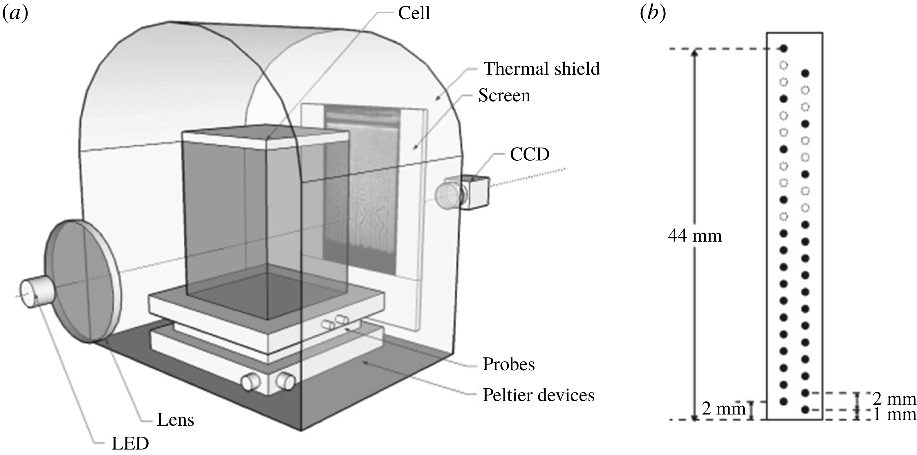
(a) Schematic of the experimental apparatus. A rectangular cell (
 $80~\text{mm}\times 80~\text{mm}\times 150$
mm) filled with aqueous ammonium chloride solution is cooled from below by an array of Peltier modules and a circulating water bath. A thermal shield regulates the ambient air temperature
 $T_{air}$
surrounding the cell such that it remains the same as the initial temperature of the solution (
 $T_{air}\approx T_{0}$
). Two optical windows are fabricated on the end walls of the shield for light transmission and hence shadowgraph imaging. (b) Sketch of the Plexiglas probe for the thermistors. The positions of the thermistor leads are shown by black dots.

2.1 The mushy-layer cell and the experimental environment
A schematic diagram of the apparatus is shown in figure 1. A rectangular cell of inner dimensions
 $80~\text{mm}\times 80~\text{mm}\times 150~\text{mm}$
that contained aqueous
 $\text{NH}_{4}\text{Cl}$
solution was cooled from below. The bottom plate of the cell was made of aluminium, and had a thickness of 8.0 mm and a square cross-section with side length of 90 mm. To inhibit chemical reactions with the working fluid, the top surface of the bottom plate was pretreated through an anodic oxidation process and coated with a thin anti-corrosion layer. Two thermistors (Honeywell, type 121-503JAJ) were installed inside the bottom plate to measure the bottom temperature
 $T_{b}$
. They were located at a distance of 2 mm from the fluid bottom surface, 20 mm apart from each other horizontally. The sidewalls of the cell were made of 8.0 mm thick Plexiglas. A nitrile–butadiene rubber O-ring was embedded between the sidewalls and the bottom plate which sealed the working fluid.
Underneath the bottom plate there was an array of Peltier devices, sandwiched between the bottom plate and base manifold made of a 30 mm thick aluminium plate. Double-spiral channels for coolant circulation were built inside the manifold. High-conductivity thermal compound was pasted between the Peltier devices and the bottom plate to enhance the thermal contact and improve the thermal homogeneity on the bottom plate. Control of the bottom-plate temperature was achieved by two cooling mechanisms (Neufeld & Wettlaufer Reference Neufeld and Wettlaufer2008; Zhong et al.
Reference Zhong, Fragoso, Wells and Wettlaufer2012). First, the Peltier devices produced a thermal gradient that was proportional to the applied electrical power, with a lower temperature on the bottom-plate side and a higher temperature on the base-manifold side. The electrical power was provided by a programmable power supply (Agilent, E3634A). Meanwhile, the aluminium base manifold maintained a constant temperature in the absence of modulation when anti-freeze coolant was circulated inside its double-spiral channel, driven by a refrigerating circulator (PolyScience, RTE-740) at a flow rate of
 $500~\text{cm}^{3}~\text{s}^{-1}$
and a cooling capacity of 900 W near
 $0\,^{\circ }\text{C}$
. Over long time scales the temperature of the manifold reached a stability of
 $0.01\,^{\circ }\text{C}$
. Over short time scales the Peltier devices provided fast control of the temperature variation on the bottom plate. In the present work, a prescribed sinusoidal variation of the bottom-plate temperature
 $$\begin{eqnarray}\displaystyle T_{b}=T_{b,0}+A\,\sin (\unicode[STIX]{x1D714}t+\unicode[STIX]{x1D719}_{0}) & & \displaystyle\end{eqnarray}$$
was maintained through the experiment, which forces growth of the overlying mushy layer with modulated rates as depicted in figure 3. Here
 $T_{b,0}$
is the initial bottom-plate temperature, whilst
 $A$
,
 $\unicode[STIX]{x1D714}$
and
 $\unicode[STIX]{x1D719}_{0}$
are the amplitude, frequency and initial phase of the modulation.
The side walls of the cell are made of 8 mm thick Plexiglas. All the cooling components (including the bottom plate, the Peltier devices and the base manifold) were enclosed from below by a Plexiglas tank filled with insulation foam. In order to further reduce the thermal disturbance from the environment, the whole apparatus was situated at the centre of a thermal shield that regulated the air temperature surrounding the cell. The thermal shield was made of a 3 mm thick aluminium plate, with a separated coolant circuit fabricated to its outer side. During the experiment, coolant from a thermal bath flowed through the circuit. The air temperature inside the shield was thus kept constant at the same initial temperature of the working fluid
 $T_{0}$
, with fluctuation less than 0.1 K during the experiment. Under typical experimental settings, the temperature inhomogeneity along the bottom plate was within 0.05 K, as measured by the two bottom-plate thermistors.
2.2 Thermometry and temperature measurements within the mushy layer
All thermometers and thermistors were calibrated in a separate calibration facility with a precision of a few millikelvin against a Hart Scientific model 5626 platinum resistance thermometer, and were traceable to the ITS-90 temperature scale. These thermometers showed excellent consistency; at the same temperature, their readings all agreed within 0.01 K. In order to obtain high-resolution temperature data within the growing mushy layer and the overlying fluid, we used a Plexiglas probe with dimensions sketched in figure 1(b). Two columns of thermistor holes were drilled inside the probe. These holes were 0.8 mm in diameter, equally spaced along each column with a spacing of 2 mm. Positions of the holes were interlaced between the two columns as shown in figure 1(b). The probe was placed inside the mushy-layer cell with its lower end against the bottom plate.
Altogether 32 calibrated thermistors were installed through the holes of the probe as indicated by the filled circles in figure 1(b). They measured the temperature with a resolution of 1 mm in a vertical range of
 $0\leqslant z\leqslant 23$
mm, and a resolution of 2 mm for
 $23\leqslant z\leqslant 44$
mm, where
 $z$
is the height above the base of the tank. These thermistors were 0.36 mm in diameter, with their metallic leads guided by the probe outside the mushy-layer cell. Supported by the two metallic leads, the tip of each thermistor was extended 2.0 cm outside the Plexiglas probe. With such a distance the thermal influence of the probe was negligible and the thermistors measured precisely the temperature of the sample fluid.
We note there were small differences in height between each thermistor and the centre of its hole due to imperfect installations. These differences were corrected in the experiment using images of the thermistors. Because of the rigidity of their supporting metallic leads, the positions of all the thermistors were not altered during the mush growth. This was evident as we found no change in their positions in the images before and after the experiment. The temperature signals of the 32 thermistors were acquired and collected by a multiple-channel data acquisition unit (Agilent, 34970A) with a sampling rate of 1 Hz. Such a sampling rate was sufficient to resolve the temperature oscillations in the mushy layer in the modulation experiments.
2.3 Image acquisition and analysis
We applied shadowgraphy to obtain images of the density field of the sample and determine the position of the mush–liquid interface. For this purpose, two transparent windows were made on the two end walls of the thermal shield for optical access (figure 1
a). A parallel beam of light was generated by an LED light located at the focus point of a convex glass lens and passed through the sample. The shadowgraph images were then projected on a translucent screen behind the mushy-layer cell, and recorded by a CCD camera at a sampling frequency of 1.875 Hz. The camera captured images of
 $1624\times 1234$
pixels with a spatial resolution of
 $15~\text{pixels}~\text{mm}^{-1}$
. Typically 30 000 images were taken in each experiment to obtain the mushy-layer thickness
 $h(t)$
with high time resolution.
Since the mush region was nearly opaque but the density variation in the liquid region was reflected in a bright area in a shadowgraphy image, the vertical position of the mush–liquid interface can be determined where the brightness contrast is maximum. In our image analysis process, a sequence of shadowgraphy images was digitized into a matrix format in which the pixel intensities
 $I(x,z)$
present distributions of brightness at the spatial coordinates
 $(x,z)$
. For each horizontal position, we then determine the vertical gradient of
 $I(x,z)$
as a function of height, using a finite difference
 $\unicode[STIX]{x0394}_{z}I=[I(x,z+\text{d}z)-I(x,z)]/\text{d}z$
, where
 $\text{d}z$
is the pixel scale. The position of the mush–liquid interface
 $h(x)$
was given where
 $\unicode[STIX]{x0394}_{z}I$
is maximum. As an example, the inset in figure 3 shows the results of our image analysis where the interface
 $h(x)$
is indicated by a green line. The horizontal average of
 $h(x)$
(red dashed line) was used to represent the mean mushy layer height in the following discussions.
2.4 Typical experimental protocol
The working fluid was an aqueous
 $\text{NH}_{4}\text{Cl}$
solution, with local temperature
 $T$
, local concentration
 $C$
and eutectic temperature
 $T_{E}$
at concentration
 $C_{E}$
. Its initial density
 $\unicode[STIX]{x1D70C}_{0}$
and temperature
 $T_{0}>T_{E}$
were measured using an oscillating-type densitometer (Anton Paar, DMA 35N). The initial concentration
 $C_{0}>C_{E}$
was then determined using the isopycnal lines of ammonium chloride based on data tables (US National Research Council 2003), with an accuracy better than
 $0.1~\text{wt}\%$
. The experimental cell (shown in figure 1
a) was pre-cooled so the bottom-plate temperature
 $T_{b}$
maintained a constant value
 $T_{b,0}=0.0\pm 0.1\,^{\circ }\text{C}$
. The solution was then carefully directed into the cell, causing a rapid increase of
 $T_{b}$
. After a short transient time (about two minutes) where
 $T_{b}$
returned to
 $0.0\,^{\circ }\text{C}$
, the temperature modulation of
 $T_{b}$
was started. We define this moment as the initial time (
 $t=t_{0}=0$
) of the measurements. Variation of
 $T_{b}$
in time followed the prescribed sinusoidal function of time (see figure 3
a). Since the liquidus temperature
 $T_{L}(C_{0})$
is higher than
 $T_{b,0}$
, the mushy-layer zone started to form at
 $t=t_{s}$
shortly after the solution filled the cell. We estimate
 $t_{s}$
by extrapolating the data of mushy-layer thickness with
 $h(t)\propto \sqrt{t-t_{s}}$
shown in figure 3(b). We find that
 $t_{s}$
is close to the initial time
 $t_{0}$
(
 $t_{s}-t_{0}\approx -20s\ll \unicode[STIX]{x1D70F}$
).
Various initial liquid concentrations
 $C_{0}$
were trialled in test experiments. We find that a greater concentration
 $C_{0}$
leads to a faster growth rate and a larger mushy-layer thickness
 $h(t)$
, since the temperature difference between the cold bottom plate and the liquidus temperature is enlarged. A large mushy-layer thickness
 $h(t)$
is desirable because it leads to more discernible differences of
 $h(t)$
between different modulation modes. However, a fast growth rate reduces the time it takes for the mushy-layer growth to reach an asymptotic state when
 $h(t)$
approaches a constant, and reduces the number of modulation periods that can be achieved at early times with sufficient growth rates. Moreover, the modulation frequency
 $\unicode[STIX]{x1D714}$
is limited to a maximum of the order of 1 mHz (dependent on the modulation amplitude
 $A$
), due to the maximum load of the Peltier devices and the finite thermal capacity of the sample. For these reasons we have chosen
 $C_{0}=29~\text{wt}\%$
and modulation periods
 $\unicode[STIX]{x1D70F}=2\unicode[STIX]{x03C0}/\unicode[STIX]{x1D714}$
with
 $2000~\text{s}\leqslant \unicode[STIX]{x1D70F}\leqslant 5000~\text{s}$
) in the experimental results presented here, which allow observations of
 $h(t)$
over several modulation periods.
3 Model of mushy-layer growth
Various continuum models of mushy-layer growth have previously been developed (e.g. Hills, Loper & Roberts Reference Hills, Loper and Roberts1983; Fowler Reference Fowler1985; Worster Reference Worster1986; Worster & Kerr Reference Worster and Kerr1994; Schulze & Worster Reference Schulze and Worster1999; Notz & Worster Reference Notz and Worster2006; Rees Jones & Worster Reference Rees Jones and Worster2014). Here we adapt a formulation by Rees Jones & Worster (Reference Rees Jones and Worster2014) to include time-dependent boundary conditions to represent the periodic cooling. We first briefly review this theoretical framework, and then present our numerical method.
3.1 Governing equation
We consider a finite region
 $0\leqslant z\leqslant H_{0}$
filled with an aqueous
 $\text{NH}_{4}\text{Cl}$
solution with initial concentration
 $C_{0}>C_{E}$
and temperature
 $T_{0}>T_{L}(C_{0})$
. Here the liquidus relation is linearized as
 $T_{L}(C)=T_{E}+\unicode[STIX]{x1D6E4}(C-C_{E})$
with assumed constant slope
 $\unicode[STIX]{x1D6E4}$
. The solution is cooled from below by the bottom plate with a time-dependent temperature lower than the initial liquidus temperature but higher than the eutectic temperature, with
 $T_{E}<T_{b}(t)<T_{L}(C_{0})$
. The solution solidifies from the bottom and forms a porous mushy region with solid fraction
 $\unicode[STIX]{x1D719}$
. Assuming the sidewalls of the sample cell are adiabatic, and horizontal transport of heat is negligible, then the temperature of the mushy layer is governed by a one-dimension heat equation (Rees Jones & Worster Reference Rees Jones and Worster2014):
 $$\begin{eqnarray}\displaystyle cp_{m}\frac{\unicode[STIX]{x2202}T}{\unicode[STIX]{x2202}t}+cp_{l}w\frac{\unicode[STIX]{x2202}T}{\unicode[STIX]{x2202}z}=\frac{\unicode[STIX]{x2202}}{\unicode[STIX]{x2202}z}\left(k_{m}\frac{\unicode[STIX]{x2202}T}{\unicode[STIX]{x2202}z}\right)+L\frac{\unicode[STIX]{x2202}\unicode[STIX]{x1D719}}{\unicode[STIX]{x2202}t}, & & \displaystyle\end{eqnarray}$$
where
 $cp$
is the volumetric heat capacity,
 $w$
is the convective velocity in the mushy layer,
 $k$
is the thermal conductivity and
 $L$
is the latent heat per unit volume. The subscript
 $m$
indicates the physical quantities in the mushy layer, which is determined by the weighted averages of the properties in each phase:
 $$\begin{eqnarray}\displaystyle & k_{m}=\unicode[STIX]{x1D719}k_{s}+(1-\unicode[STIX]{x1D719})k_{l}, & \displaystyle\end{eqnarray}$$
 $$\begin{eqnarray}\displaystyle & cp_{m}=\unicode[STIX]{x1D719}cp_{s}+(1-\unicode[STIX]{x1D719})cp_{l}. & \displaystyle\end{eqnarray}$$
 $l$
and
 $s$
denote values in the liquid and solid, respectively. We assume local thermodynamic equilibrium is satisfied within the mushy layer, so the temperature and concentration are related according to the liquidus relation
 $T=T_{L}(C)$
. The local solid fraction within the mushy layer is determined through conservation of solute. We assume that vertical solute transport has a negligible impact, so that the local phase-weighted bulk concentration
 $S(z)=C_{s}\unicode[STIX]{x1D719}+(1-\unicode[STIX]{x1D719})C(z)$
is given by
 $C_{0}$
, where the concentration of the solid
 $C_{s}\approx 1$
. Thus the local solid fraction
 $\unicode[STIX]{x1D719}$
can be determined from
 $\unicode[STIX]{x1D719}=[C_{0}-C(z)]/[1-C(z)]$
. In reality, this approximation will degrade over time as the bulk concentration evolves due to neglected convective solute fluxes from the mushy layer. We also assume that the fluid temperature maintains a constant value
 $T_{l}=T_{0}$
in the liquid region far above the mushy layer. The thickness
 $h(t)$
of the mushy layer is determined by the position of the front of solidification, which is controlled by the heat flux balance at the interface
 $$\begin{eqnarray}\displaystyle cp_{l}[T_{l}-T_{L}(C_{i})]\left(\frac{\text{d}h}{\text{d}t}-w|_{z=h}\right)+\unicode[STIX]{x1D719}_{i}L\frac{\text{d}h}{\text{d}t}+F_{T}=\left.k_{m}\frac{\unicode[STIX]{x2202}T}{\unicode[STIX]{x2202}z}\right|_{z=h}, & & \displaystyle\end{eqnarray}$$
where
 $F_{T}$
is the turbulent heat flux at the mush–liquid interface,
 $\unicode[STIX]{x1D719}_{i}$
is the interfacial solid fraction and
 $C_{i}$
is the interfacial concentration (determined below). We denote the concentration of the liquid region as
 $C_{l}$
, which is well approximated by
 $C_{l}\approx C_{0}$
at early times before the accumulation of considerable solute fluxes from the mushy layer. Since aqueous
 $\text{NH}_{4}\text{Cl}$
solutions with
 $C_{0}>C_{E}$
are used as the working fluid, there is an overall stabilizing temperature gradient in both the mush and liquid region. However, due to compositional convection, cold and fresh fluid at the mush–liquid interface can rise above the compositional boundary layer and into the melt. The temperature of these plumes adjusts from the interfacial temperature
 $T_{i}$
to the far-field fluid temperature
 $T_{0}$
over a length scale determined by the balance of thermal diffusion and vertical advection due to flow from the compositional convection. Following Woods & Huppert (Reference Woods and Huppert1989), the turbulent heat flux is related to the compositional flux
 $F_{C}$
through
 $$\begin{eqnarray}\displaystyle F_{T}=cp_{l}\frac{[T_{l}-T_{L}(C_{i})]}{[C_{l}-C_{i}]}F_{C}, & & \displaystyle\end{eqnarray}$$
where
 $F_{C}$
is determined by
 $$\begin{eqnarray}\displaystyle F_{C}=2^{4/3}\unicode[STIX]{x1D706}D\left(\frac{\unicode[STIX]{x1D6FD}_{C}g}{D\unicode[STIX]{x1D708}}\right)^{1/3}(C_{l}-C_{i})^{4/3}, & & \displaystyle\end{eqnarray}$$
with
 $\unicode[STIX]{x1D706}$
the heat transfer coefficient,
 $D$
the solute diffusivity,
 $\unicode[STIX]{x1D6FD}_{C}$
the solute expansion coefficient,
 $g$
the gravitational acceleration and
 $\unicode[STIX]{x1D708}$
the kinematic viscosity. The heat transfer coefficient
 $\unicode[STIX]{x1D706}$
is dependent on the convection forcing, the buoyancy ratio and the physical properties of the working fluid (Yang, Verzicco & Lohse Reference Yang, Verzicco and Lohse2016, for example). We thus expect that its best parameterization varies in diverse experimental systems (Turner Reference Turner1979; Worster & Kerr Reference Worster and Kerr1994; Wettlaufer et al.
Reference Wettlaufer, Worster and Huppert1997; Rees Jones & Worster Reference Rees Jones and Worster2014; Huguet et al.
Reference Huguet, Alboussiere, Bergman, Deguen, Labrosse and Lesceur2016). In our numerical treatments, we select the optimized value of
 $\unicode[STIX]{x1D706}=0.1$
such that the predicted oscillation amplitude of
 $\unicode[STIX]{x1D6FF}h$
best matches the experimental data shown in figures 3 and 4. Whilst we include the impact of compositional convection on heat transfer at the mush–liquid interface, we assume that the liquid concentration and temperature far above the mush hardly change due to the comparatively large reservoir of fluid.
The compositional heat transport at the mush–liquid interface in (3.4) and (3.5) depends on the concentration difference between the mush–liquid interface and the far-field liquid. Assuming local thermodynamic equilibrium holds in the mushy layer and the bulk concentration is conserved with
 $\unicode[STIX]{x1D719}_{i}C_{s}+(1-\unicode[STIX]{x1D719}_{i})C_{i}=C_{0}$
, then the presence of a solutal difference with
 $C_{i}<C_{l}=C_{0}$
implies a finite solid fraction
 $\unicode[STIX]{x1D719}_{i}=(C_{0}-C_{i})/(C_{s}-C_{i})>0$
at the mush–liquid interface. In principle, one could estimate
 $C_{i}$
from the solute budget at the mush–liquid interface. In practice, the compositional fluxes may depend on microscopic details of solute depletion and plume production at the dendrite tips, which are not fully accounted for in the scalings (3.4) and (3.5). Furthermore, these dynamics occur in a region where the spacing between dendrite tips becomes sparse for small
 $\unicode[STIX]{x1D719}$
, and hence the assumption of local thermodynamic equilibrium will be least accurate there. (In the mush interior, pore-scale solutal gradients drive local phase change that relaxes to local thermodynamic equilibrium faster than the time scale of macroscopic transport, but such gradients will interact with the small-scale compositional convection at the dendrite tips.) We therefore take a pragmatic approach, that has been adopted in some sea-ice models (Turner, Hunke & Bitz Reference Turner, Hunke and Bitz2013), and fit a value of
 $\unicode[STIX]{x1D719}_{i}=\unicode[STIX]{x1D719}_{c}$
for the interfacial solid fraction. In the present model, we determine
 $\unicode[STIX]{x1D719}_{c}=0.008$
by the best fitting of the experimental data for the initial growth rate of the mushy layer in the early period (figure 3
b). Note that this procedure effectively fits the strength of the compositional convection from the liquid region, as determined by
 $\unicode[STIX]{x1D719}_{i}$
and thus
 $C_{i}$
. For simplicity, we also assume that heat transfer via the mushy-layer mode of convection is weak compared to that driven by compositional convection at the interface, and approximate
 $w=0$
. As thermal equilibrium is reached at the mush–liquid interface,
 $T_{i}$
is then determined from
 $C_{i}$
through the liquidus relation. In summary, the resulting boundary condition at the mush–liquid interface is given by
 $$\begin{eqnarray}\displaystyle \unicode[STIX]{x1D719}_{i}=\unicode[STIX]{x1D719}_{c},\quad C(h)=C_{i}=\frac{C_{o}-\unicode[STIX]{x1D719}_{i}}{1-\unicode[STIX]{x1D719}_{i}},\quad T(h)=T_{i}=T_{L}(C_{i}). & & \displaystyle\end{eqnarray}$$
Equations (3.1), interfacial boundary conditions (3.3)–(3.6) and basal boundary condition (2.1) constitute the governing equations for the growth of the mushy layer. If the thermal properties of the mushy layer (
 $L,cp_{m}$
and
 $k$
) are treated as constants, we recover a Stefan problem with mushy-layer thickness
 $h\,\propto \,t^{1/2}$
when the cooling boundary temperature is a constant (Huppert & Worster Reference Huppert and Worster1985). In this work, we consider that the cooling temperature varies periodically as a sinusoidal function given by (2.1), so that growth departs from the classical scaling
 $h\propto t^{1/2}$
. Due to the time-varying boundary temperature and material properties varying with
 $z$
, we here solve the system numerically.
3.2 Numerical method
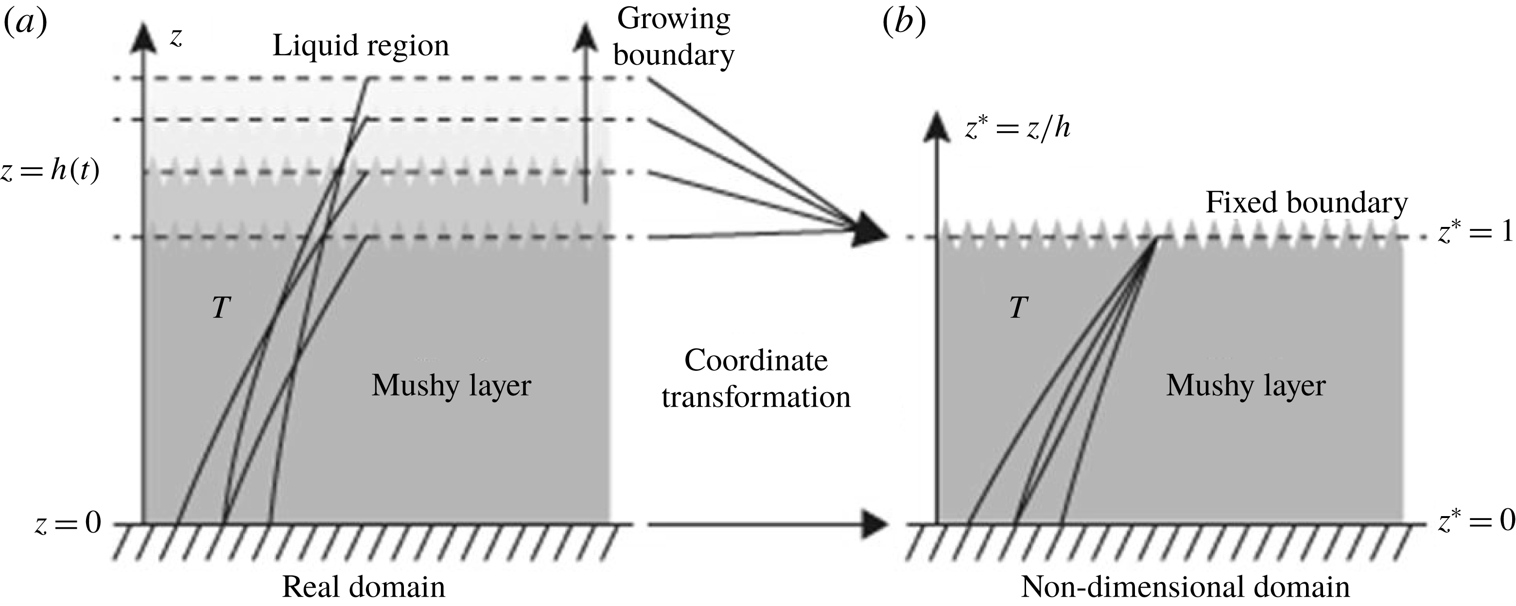
Illustration of the coordinate transformation method we apply in the numerical calculations. Temperature profiles are sketched as black curves in the real mushy-layer domain (a) and in the non-dimensional domain (b).

As the solid fraction
 $\unicode[STIX]{x1D719}$
is coupled with temperature and concentration, the temporal derivative of
 $\unicode[STIX]{x1D719}$
can be written as
 $$\begin{eqnarray}\displaystyle \frac{\unicode[STIX]{x2202}\unicode[STIX]{x1D719}}{\unicode[STIX]{x2202}t}=-\frac{(1-C_{0})}{\unicode[STIX]{x1D6E4}(1-C)^{2}}\frac{\unicode[STIX]{x2202}T}{\unicode[STIX]{x2202}t}. & & \displaystyle\end{eqnarray}$$
Thus, the governing equation (3.1) can be simplified as
 $$\begin{eqnarray}\displaystyle cp_{e}\frac{\unicode[STIX]{x2202}T}{\unicode[STIX]{x2202}t}=\frac{\unicode[STIX]{x2202}}{\unicode[STIX]{x2202}z}\left(k_{m}\frac{\unicode[STIX]{x2202}T}{\unicode[STIX]{x2202}z}\right), & & \displaystyle\end{eqnarray}$$
where
 $cp_{e}=cp_{m}+L(1-C_{0})/[\unicode[STIX]{x1D6E4}(1-C)^{2}]$
is the effective heat capacity (cf. Feltham et al.
Reference Feltham, Untersteiner, Wettlaufer and Worster2006). In the numerical calculations we transformed the mushy-layer region from an evolving domain
 $(0\leqslant z\leqslant h(t))$
to a fixed domain
 $(0\leqslant z^{\ast }\leqslant 1)$
(following Yao & Prusa Reference Yao and Prusa1989; Rizwan-Uddin 1999, for example). The coordinate transformation in this non-dimensionalization approach is illustrated in figure 2. We introduce
 $$\begin{eqnarray}\displaystyle z^{\ast }=z/h,\quad t^{\ast }=\frac{tk_{l}}{H_{0}^{2}cp_{l}},\quad h^{\ast }=h/H_{0},\quad \unicode[STIX]{x1D703}^{\ast }=\frac{T-T_{b,0}}{\unicode[STIX]{x0394}T}, & & \displaystyle\end{eqnarray}$$
where
 $H_{0}$
is the height of the cell and
 $\unicode[STIX]{x0394}T=T_{L}(C_{0})-T_{b,0}$
. After non-dimensionalization the thickness of the mushy layer becomes explicit, and
 $h$
can be evolved using the dimensionless form of the Stefan condition below. The initial thickness of the mushy layer is
 $h=0$
, and division by
 $h$
yields a singularity if
 $h=0$
. To overcome this problem, we instead use
 $\unicode[STIX]{x1D709}=(h^{\ast })^{2}$
when solving for the thickness of the mushy layer (following Rees Jones & Worster Reference Rees Jones and Worster2014). Neglecting the small difference in density between liquid and solid and dropping the asterisks of the non-dimensional variables, the dimensionless governing equation reads
 $$\begin{eqnarray}\displaystyle \unicode[STIX]{x1D709}\unicode[STIX]{x1D703}_{t}-\frac{z}{2}\dot{\unicode[STIX]{x1D709}}\unicode[STIX]{x1D703}_{z}=\frac{cp_{l}}{cp_{e}}\frac{\unicode[STIX]{x2202}}{\unicode[STIX]{x2202}z}\left(\frac{k_{m}}{k_{l}}\frac{\unicode[STIX]{x2202}\unicode[STIX]{x1D703}}{\unicode[STIX]{x2202}z}\right). & & \displaystyle\end{eqnarray}$$
The boundary conditions can be written as
 $$\begin{eqnarray}\displaystyle & \displaystyle [\unicode[STIX]{x1D703}_{l}-\unicode[STIX]{x1D703}_{L}(C_{i})+\unicode[STIX]{x1D719}_{i}St]\frac{\dot{\unicode[STIX]{x1D709}}}{2}+\unicode[STIX]{x1D709}^{1/2}Nu=\frac{k_{m}}{k_{l}}\left|\unicode[STIX]{x1D703}_{z}\right|_{z=1}\!, & \displaystyle\end{eqnarray}$$
 $$\begin{eqnarray}\displaystyle & \displaystyle \unicode[STIX]{x1D703}_{z=0}=\frac{A}{\unicode[STIX]{x0394}T}\sin (\unicode[STIX]{x1D714}t+\unicode[STIX]{x1D719}_{0}), & \displaystyle\end{eqnarray}$$
 $$\begin{eqnarray}\displaystyle & \displaystyle \unicode[STIX]{x1D703}_{z=1}=\frac{T_{L}(C_{i})-T_{b,0}}{\unicode[STIX]{x0394}T}, & \displaystyle\end{eqnarray}$$
 $St=L/cp_{l}\unicode[STIX]{x0394}T$
and
 $$\begin{eqnarray}\displaystyle Nu=2^{4/3}\unicode[STIX]{x1D706}D\frac{cp_{l}H_{0}}{k_{l}}\left(\frac{\unicode[STIX]{x1D6FD}_{C}g}{D\unicode[STIX]{x1D708}}\right)^{1/3}\frac{[T_{l}-T_{L}(C_{i})]}{\unicode[STIX]{x0394}T}(C_{l}-C_{i})^{1/3}. & & \displaystyle\end{eqnarray}$$
The complete model includes (3.10) which governs the temperature field, the Stefan condition (3.11a
) which determines the growth rate of the mushy layer and boundary conditions (3.11b
) and (3.11c
) for temperature. For every time step, the temperature profile and
 $\unicode[STIX]{x1D709}$
were updated in two steps. Firstly
 $\unicode[STIX]{x1D709}$
was updated by solving the Stefan condition (3.11a
) with a fourth-order Runge–Kutta method. The heat equation (3.10) was discretized with a forward difference scheme for the temporal derivative and a central difference scheme for the spatial derivative. Secondly the tridiagonal matrix obtained from the discretization was solved by the Thomas method (Conte & Boor Reference Conte and Boor1989) with the boundary conditions (3.11b
) and (3.11c
) and the updated results for
 $h$
and
 ${\dot{h}}$
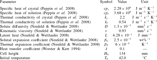
, and the temperature profile was renewed. The parameters used in the model are listed in table 1.
The parameter values used in the model.

4 Results of mushy-layer growth
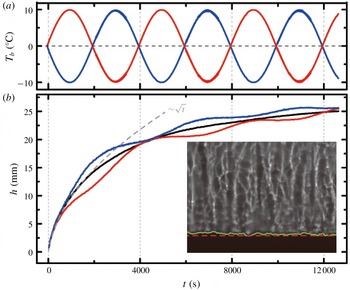
(a) The bottom-plate temperatures
 $T_{b}(t)$
as a function of time. Results for
 $A=10~\text{K}$
,
 $\unicode[STIX]{x1D70F}=4000~\text{s}$
,
 $\unicode[STIX]{x1D719}_{0}=0$
(red curve) and
 $\unicode[STIX]{x1D719}_{0}=\unicode[STIX]{x03C0}$
(blue curve) and for
 $A=0$
(black curve). (b) The height of the mushy layer as a function of time. The dashed curve shows a fitting to the initial growth in the constant-cooling mode:
 $h(t)=2\unicode[STIX]{x1D6EC}(Dt)^{1/2}$
with
 $D$
the solute diffusivity and the coefficient
 $\unicode[STIX]{x1D6EC}=4.85$
. The vertical dashed lines indicate the time at which each modulation period begins. Inset: a shadowgraph image focusing on the mush–liquid interface. The green solid line shows the position of the mush–liquid interface identified by our image processing system. The red dashed line represents the mean height of the mushy layer.

The relative mushy-layer height
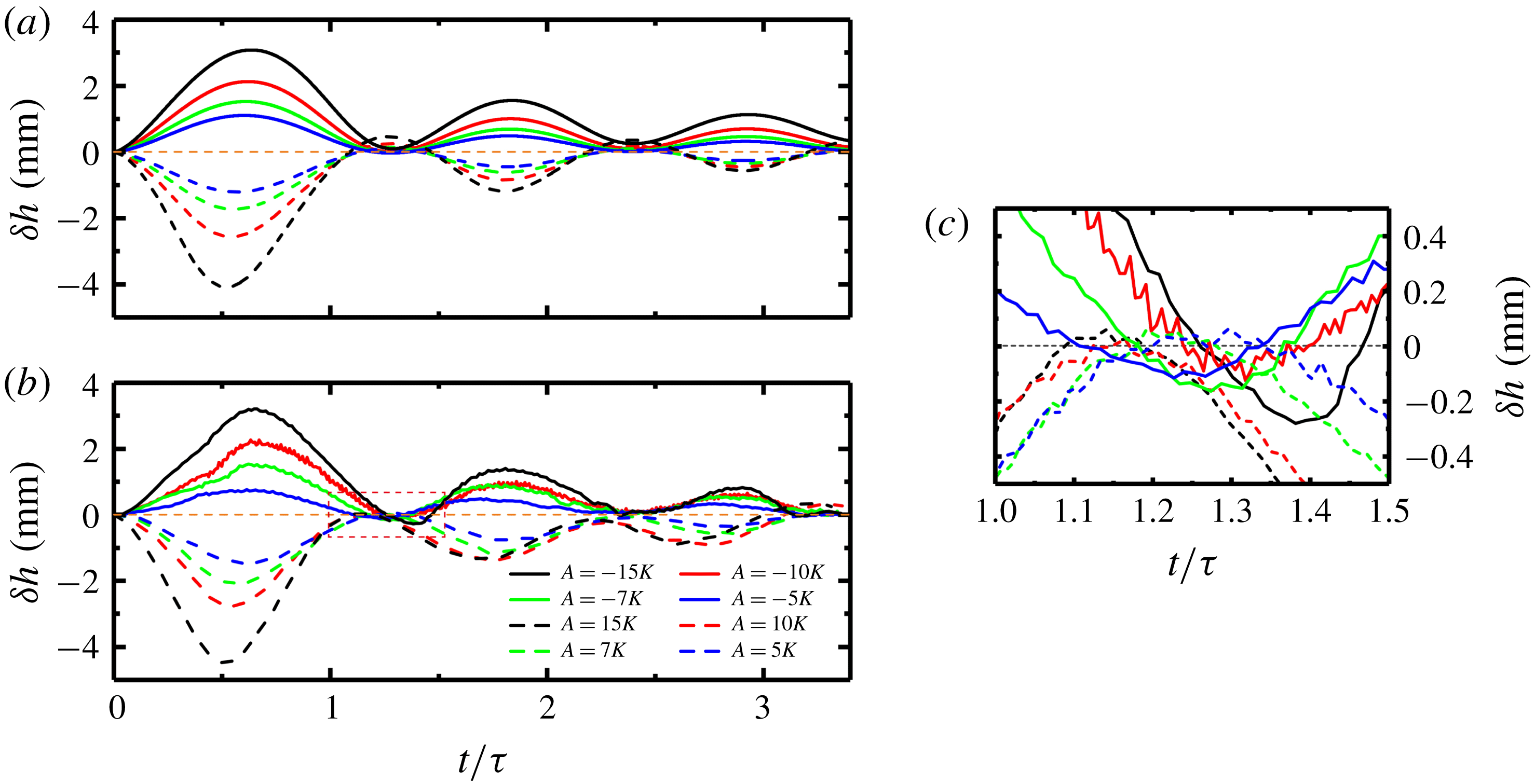
 $\unicode[STIX]{x1D6FF}h=h(t)-h_{0}$
as a function of time for different modulation amplitudes and phases. Results for
 $\unicode[STIX]{x1D70F}=4000~\text{s}$
and
 $5.0~\text{K}\leqslant A\leqslant 15.0~\text{K}$
. Solid lines:
 $\unicode[STIX]{x1D719}_{0}=\unicode[STIX]{x03C0}$
; dashed lines:
 $\unicode[STIX]{x1D719}_{0}=0$
. Results from (a) the numerical model and (b) the experiment. (c) An expanded view of the experimental data in the region with
 $1.0\leqslant t/\unicode[STIX]{x1D70F}\leqslant 1.5$
.

Figure 3 shows one representative experimental result for mushy-layer growth. The height
 $h(t)$
of the mushy layer is sensitive to the temperature variation of the cooling boundary. Here we compare results of
 $h(t)$
in three different growth modes according to the phase of the temperature modulation: (i) the initially negative modulation mode that has an initial phase
 $\unicode[STIX]{x1D719}_{0}=\unicode[STIX]{x03C0}$
, (ii) the initially positive modulation mode with
 $\unicode[STIX]{x1D719}_{0}=0$
and (iii) the constant-cooling mode with
 $A=0$
. If
 $T_{b}$
is maintained constant, the mushy layer grows initially in the well-known transient mode where the thickness evolves approximately as the square root of time
 $h_{0}(t)\propto t^{1/2}$
, with considerable deviation at late times due to turbulent heat flux in the liquid (cf. Wettlaufer et al.
Reference Wettlaufer, Worster and Huppert1997). When
 $T_{b}$
oscillates periodically, however, the applied temperature modulation clearly impacts the growth rate of the mushy layer. Depending on the initial phase
 $\unicode[STIX]{x1D719}_{0}$
, peaks and troughs appear on the growth curves
 $h(t)$
alternately. Interestingly, the growth curve in the constant-cooling mode
 $h_{0}(t)$
provides approximately an upper envelope on the growth curve
 $h(t)$
in the negative modulation mode and a lower envelope on the positive modulation mode. These reveal the time-integrated cooling (warming) effect on the mushy-layer growth. In the negative mode when
 $\unicode[STIX]{x1D719}_{0}=\unicode[STIX]{x03C0}$
,
 $T_{b}$
initially decreases and is negative in the first half of the modulation period. The mushy layer undergoes extra cooling and hence the growth rate increases. In the second half of the modulation period,
 $T_{b}$
increases and exceeds
 $T_{0}$
, the mushy layer is relatively warm and the growth rate decreases until
 $h(t)$
approaches
 $h_{0}(t)$
. As a result we observe peaks that are superimposed above the growth curve
 $h_{0}(t)$
. In the positive mode with
 $\unicode[STIX]{x1D719}_{0}=0$
, however,
 $T_{b}$
first increases, and the growth rate first decreases and troughs appear. We find in this mode
 $h(t)$
mostly underlays
 $h_{0}(t)$
. The magnitudes of the peaks and troughs both decrease in time. After a sufficiently long time (more than three modulation periods), effects of periodic cooling on the mushy-layer growth rates weaken, and the growth curves in both modulation modes begin to approach
 $h_{0}(t)$
at long time.
Figures 4 and 5 depict the numerical and experimental results of the relative height,
 $\unicode[STIX]{x1D6FF}h=h(t)-h_{0}(t)$
, of a thermally modulated run with height
 $h(t)$
as a function of time, compared to a run with fixed temperature (
 $A=0$
) with height
 $h_{0}(t)$
. They clearly illustrate the magnitudes of the peaks and troughs on the growth curves. Figure 4 shows the results for a modulation period
 $\unicode[STIX]{x1D70F}=4000~\text{s}$
, but with different modulation amplitudes in the range of
 $5.0~\text{K}\leqslant A\leqslant 15.0~\text{K}$
. When a larger modulation amplitude
 $A$
is applied, larger relative height
 $\unicode[STIX]{x1D6FF}h$
is observed. Moreover, the reductions in
 $h(t)$
are greater in the positive mode (
 $\unicode[STIX]{x1D719}_{0}=0$
, dashed curves) than the corresponding enhancements in the negative mode (
 $\unicode[STIX]{x1D719}_{0}=\unicode[STIX]{x03C0}$
, solid curves), observed in both the experimental data and the numerical results. Such an asymmetry is most evident with the largest modulation amplitude in the first modulation period. It implies that increasing the cooling temperature of the bottom plate has a stronger influence on the growth rate than otherwise decreasing
 $T_{b}$
by the same amount.
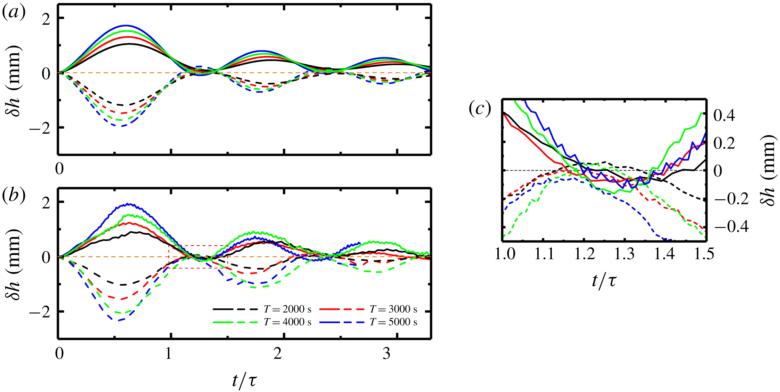
The relative mushy-layer height
 $\unicode[STIX]{x1D6FF}h=h(t)-h_{0}$
as a function of time for different modulation periods. Results for
 $A=7~\text{K}$
and
 $2000~\text{s}\leqslant \unicode[STIX]{x1D70F}\leqslant 5000~\text{s}$
. Solid lines:
 $\unicode[STIX]{x1D719}_{0}=\unicode[STIX]{x03C0}$
; dashed lines:
 $\unicode[STIX]{x1D719}_{0}=0$
. (a) Numerical model and (b) experimental results. (c) An expanded view of the experimental data in the region with
 $1.0\leqslant t/\unicode[STIX]{x1D70F}\leqslant 1.5$
.

Figure 5 shows the relative height
 $\unicode[STIX]{x1D6FF}h$
for a given modulation amplitude
 $A=7~\text{K}$
and varying modulation periods, plotted as a function of
 $t/\unicode[STIX]{x1D70F}$
to normalize by the period. It is clear that a larger modulation period
 $\unicode[STIX]{x1D70F}$
leads to a larger
 $\unicode[STIX]{x1D6FF}h$
over the range studied (
 $2000~\text{s}\leqslant \unicode[STIX]{x1D70F}\leqslant 5000~\text{s}$
). Our qualitative interpretation is that the magnitude of the peaks (troughs) of
 $h(t)$
is given by accumulation of the extra cooling (or warming) that the fluid undergoes during the previous part of the modulation period, compared to that in a constant-cooling mode (
 $A=0$
). When a larger modulation period is applied, the fluid layer is subjected to a longer period of extra cooling (warming) and the acceleration (deceleration) in
 $h(t)$
lasts for longer. Therefore,
 $\unicode[STIX]{x1D6FF}h$
is greater for longer modulation periods or larger amplitude modulation. This is one of the central observations in the present study. In § 5 we examine this phenomenon further, providing a quantitative analysis of how the mushy-layer growth curve is influenced by the modulation frequency and elucidating the frequency dependence of the relative heights observed in the experiment.
The oscillations of
 $T_{b}$
induce nearly periodically spaced peaks (troughs) on the growth curves
 $h(t)$
. The antinodes where
 $\unicode[STIX]{x1D6FF}h$
is maximal lag behind the phase of corresponding nodes in modulation of the basal temperature (compare to dashed lines in figure 3
b). When the mushy-layer thickness increases, the thermal gradient at the mush–liquid interface, which determines the growth rate, takes longer to respond to the temperature variations of
 $T_{b}$
. This is likely due to the larger thermal diffusion time scale
 $\unicode[STIX]{x1D70F}_{d}\sim h^{2}/\unicode[STIX]{x1D6FC}$
, where
 $\unicode[STIX]{x1D6FC}=k_{m}/cp_{e}$
is the thermal diffusivity. As a result, it takes a certain delay time for the growth rate to increase after
 $T_{b}$
starts to decrease, leading to a phase lag of
 $h(t)$
versus
 $T_{b}(t)$
. The phase lag continues to increase in time as illustrated in figures 3–5.
One important feature of the theoretically predicted growth curves shown in figures 4(a) and 5(a) is that the relative height
 $\unicode[STIX]{x1D6FF}h(t)$
may change signs near the nodes, i.e.
 $h(t)$
may drop below (rise above)
 $h_{0}(t)$
in a negative (positive) modulation mode. Such an ‘overshooting’ behaviour is sometimes captured as well in the experimental data curves (figures 4
c and 5
c). Our numerical analysis suggests that this phenomenon is mainly attributed to the variation of conduction through the mushy layer, which drives growth, versus turbulent heat transport at the mush–liquid interface, which suppresses the growth rate. This effect is directly revealed in (3.11a
) where the growth rate depends on
 $\unicode[STIX]{x1D709}^{1/2}Nu$
(or
 $h^{\ast }Nu$
) which represents the ratio of the interfacial heat flux to a conductive heat flux over a mushy-layer thickness
 $h$
. The mushy-layer height is smaller on average during the positive modulation mode than in the constant-cooling mode, corresponding to a larger conductive heat flux
 $\propto k_{m}\unicode[STIX]{x0394}T/h$
. Thus
 $hNu$
becomes less than
 $h_{0}Nu$
and allows a larger growth rate during the positive modulation mode. In certain parameter regimes where the interfacial heat flux is dominant,
 $h(t)$
may rise above
 $h_{0}(t)$
at some modulation phases. In a negative growth mode, however, the mushy-layer height is larger on average, and reduces the conductive heat flux compared to the interfacial heat flux, which in turn reduces the growth rate. At certain modulation phases,
 $h(t)$
drops below
 $h_{0}(t)$
. At very large times with
 $t\gg \unicode[STIX]{x1D70F}$
, the conductive heat flux in a modulation mode becomes the same as in the constant-cooling mode since
 $h(t)$
approaches
 $h_{0}(t)$
. Thus the overshooting effect diminishes as shown in figures 4 and 5.
5 Theoretical scaling for early-time growth with periodic cooling
In this section, we develop scaling arguments to understand the modulation of mushy-layer thickness in the experimental observations and numerical model. We use the heat equation (3.8), noting that we can express
 $cp_{e}$
as
 $$\begin{eqnarray}\displaystyle cp_{e}=cp_{m}+(1-\unicode[STIX]{x1D719})\frac{L}{[T_{L}(C_{S})-T]}, & & \displaystyle\end{eqnarray}$$
which is an effective heat capacity accounting for latent heat release during internal solidification. Whilst
 $cp_{e}$
and
 $k_{m}$
generally vary with temperature and solid fraction, we approximate them by constant representative values for the scaling arguments in this section. Writing
 $\unicode[STIX]{x1D719}=[C_{0}-C]/[C_{S}-C]=[T_{L}(C_{0})-T]/[T_{L}(C_{S})-T]$
and using the thermal boundary conditions we can bound
 $0\leqslant \unicode[STIX]{x1D719}\leqslant [T_{L}(C_{0})-T_{b,0}]/[T_{L}(C_{S})-T_{b,0}]$
for growth without modulated cooling
 $(A=0)$
. For
 $\unicode[STIX]{x1D6E4}=4.72\,^{\circ }\text{C}~\text{wt}\%^{-1}$
,
 $T_{E}=-15.4\,^{\circ }\text{C}$
and
 $C_{E}=19.7~\text{wt}\%$
(Neufeld & Wettlaufer Reference Neufeld and Wettlaufer2008), then
 $C_{S}=100~\text{wt}\%$
,
 $C_{0}=29~\text{wt}\%$
, and
 $T_{b,0}=0\,^{\circ }\text{C}$
yields
 $0\leqslant \unicode[STIX]{x1D719}\leqslant 0.08$
. We use the upper bound
 $\unicode[STIX]{x1D719}=0.08$
in subsequent estimates, and take
 $T=T_{b,0}$
when calculating
 $cp_{e}$
. Combining these values with those in table 1 results in representative estimates
 $cp_{e}=4.7\times 10^{-3}~\text{J}~\text{mm}^{-3}~\text{K}^{-1}$
and
 $k_{m}=6.7\times 10^{-4}~\text{J}~\text{mm}^{-1}~\text{s}^{-1}~\text{K}^{-1}$
, from which we infer an effective thermal diffusivity
 $\unicode[STIX]{x1D6FC}=k_{m}/cp_{e}\approx 0.14~\text{mm}^{2}~\text{s}^{-1}$
.
We identify three key time scales for the growing mushy layer: the modulation period
 $\unicode[STIX]{x1D70F}=2\unicode[STIX]{x03C0}/\unicode[STIX]{x1D714}$
, the diffusion time scale
 $t_{d}\sim h^{2}/\unicode[STIX]{x1D6FC}$
across the mushy-layer thickness and a diffusively controlled equilibration time scale
 $t_{s}\sim h_{s}^{2}/\unicode[STIX]{x1D6FC}$
for an approach to the steady-state mush thickness
 $h_{s}$
in the absence of modulation. The steady-state thickness results from the approximate balance
 $F_{T}\sim k_{m}\unicode[STIX]{x0394}T/h_{s}$
in (3.3) between the turbulent heat flux in the liquid, and conduction through the mush, where
 $\unicode[STIX]{x0394}T=T_{L}(C_{i})-T_{b}$
is a scale for temperature differences across the mushy layer. To yield a tractable analysis that captures the essence of the problem, we consider a scenario where at early times the mushy layer is sufficiently far from the steady state for
 $t_{d}\ll t_{s}$
, yielding
 $h^{2}/h_{s}^{2}\ll 1$
. We also assume that the diffusive time scale
 $t_{d}$
is either smaller than or comparable to the modulation period
 $\unicode[STIX]{x1D70F}$
, yielding
 $\unicode[STIX]{x1D714}h^{2}/\unicode[STIX]{x1D6FC}\lesssim 1$
. Finally, at long times the steady state (or modulated form thereof) is approached with
 $h\rightarrow h_{s}$
. In practice the separation of time scales is not very strong for the present experimental configuration, which is in a crossover regime where all of
 $\unicode[STIX]{x1D70F}$
,
 $t_{d}$
and
 $t_{s}$
are of similar order for much of the experiment. For example, for modulation with
 $\unicode[STIX]{x1D70F}=4000~\text{s}$
, figure 3(a) shows
 $h\approx 15~\text{mm}$
near the first local extrema in
 $\unicode[STIX]{x1D6FF}h$
at
 $t=2000~\text{s}$
, versus a steady-state thickness of
 $h_{s}\approx 30~\text{mm}$
. This early-time case corresponds to
 $\unicode[STIX]{x1D714}h^{2}/\unicode[STIX]{x1D6FC}\approx 2.5$
and
 $h^{2}/h_{s}^{2}\approx 0.25$
. We will nevertheless pursue scaling arguments for the regimes with
 $h^{2}/h_{s}^{2}\ll 1$
and
 $\unicode[STIX]{x1D714}h^{2}/\unicode[STIX]{x1D6FC}\lesssim 1$
. This will provide physical insight that is useful for interpreting the present experiment, but also for the behaviour expected as conditions vary beyond the range considered here.
At early times
 $\unicode[STIX]{x1D714}h^{2}/\unicode[STIX]{x1D6FC}\lesssim 1$
and
 $h^{2}/h_{s}^{2}\ll 1$
. In this limit, the modulation is either relatively slow
 $(\unicode[STIX]{x1D70F}\gg t_{d})$
or similar compared to the diffusion time scale, and there is sufficient time for variations in the basal temperature to diffuse through the full depth of the mushy layer. The dominant thermal gradients will therefore occur over a length scale commensurate with the mushy-layer thickness
 $h$
(cf. figure 10). Hence the heat flux driving growth scales as
 $k_{m}\unicode[STIX]{x2202}T/\unicode[STIX]{x2202}z|_{z=h}\sim \unicode[STIX]{x1D702}k_{m}\unicode[STIX]{x0394}T/h$
, with
 $\unicode[STIX]{x0394}T\approx T_{L}(C_{i})-T_{b}=\unicode[STIX]{x0394}T_{0}-A\sin (\unicode[STIX]{x1D714}t+\unicode[STIX]{x1D719}_{0})$
depending on the modulated temperature,
 $\unicode[STIX]{x0394}T_{0}=T_{L}(C_{i})-T_{b,0}$
and
 $\unicode[STIX]{x1D702}$
a constant of proportionality of order one. The condition
 $h\ll h_{s}$
also implies we can neglect the turbulent flux
 $F_{T}\ll k_{m}\unicode[STIX]{x0394}T/h$
. Then the Stefan condition (3.3) reduces to
 $$\begin{eqnarray}\displaystyle \{cp_{l}[T_{l}-T_{L}(C_{i})]+L\unicode[STIX]{x1D719}_{i}\}\frac{\text{d}h}{\text{d}t}\sim \unicode[STIX]{x1D702}\frac{k_{m}}{h}[\unicode[STIX]{x0394}T_{0}-A\sin (\unicode[STIX]{x1D714}t+\unicode[STIX]{x1D719}_{0})], & & \displaystyle\end{eqnarray}$$
which corresponds to a quasi-steady response of the mushy layer to the instantaneous basal temperature. Integrating (5.2) yields
 $$\begin{eqnarray}\displaystyle h^{2}\sim \frac{2\unicode[STIX]{x1D702}}{{\mathcal{S}}}\left[\unicode[STIX]{x1D6FC}t+\frac{\unicode[STIX]{x1D6FC}}{\unicode[STIX]{x1D714}}\frac{A}{\unicode[STIX]{x0394}T_{0}}\cos (\unicode[STIX]{x1D714}t+\unicode[STIX]{x1D719}_{0})\right],\quad {\mathcal{S}}=\frac{cp_{l}[T_{l}-T_{L}(C_{i})]+L\unicode[STIX]{x1D719}_{i}}{cp_{e}\,\unicode[STIX]{x0394}T_{0}}, & & \displaystyle\end{eqnarray}$$
where the modified Stefan number
 ${\mathcal{S}}$
is defined by the second equality. In the absence of modulation
 $(A=0)$
we obtain the square-root-of-time growth characteristic of the classical Stefan problem, with
 $h=h_{0}(t)\sim \sqrt{2\unicode[STIX]{x1D702}\unicode[STIX]{x1D6FC}t/{\mathcal{S}}}$
. The correction due to modulation of the boundary temperature satisfies
 $h^{2}-h_{0}^{2}\propto A/\unicode[STIX]{x1D714}$
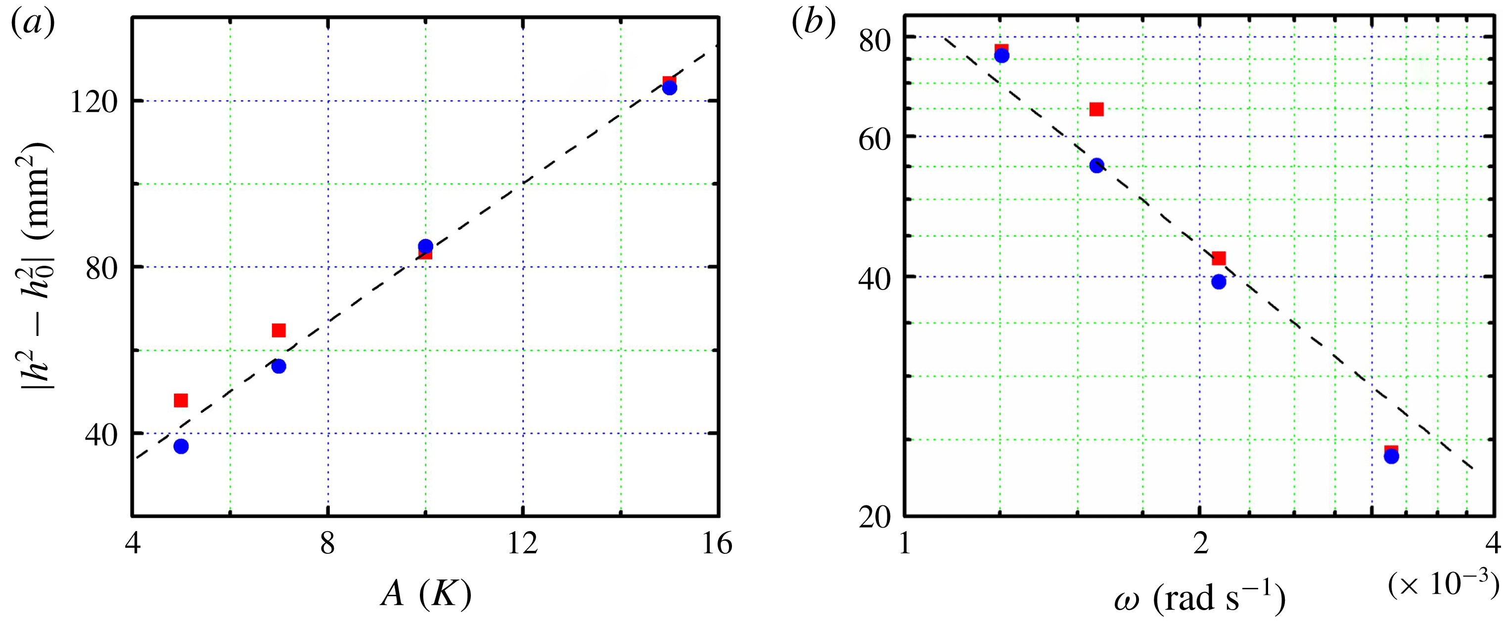
. This scaling is consistent with data in figure 6, which shows the distances
 $|h^{2}-h_{0}^{2}|$
measured at the first peak and trough as a function of the modulation amplitude and frequency. Here
 $h_{0}(t)$
is determined from the experimental data without boundary modulation.
(a) The distances
 $|h^{2}-h_{0}^{2}|$
measured at the first peak (trough) as a function of the modulation amplitude. Results for
 $\unicode[STIX]{x1D70F}=4000~\text{s}$
. The dashed line shows a proportional relation:
 $|h^{2}-h_{0}^{2}|=8.35A~(\text{mm}^{2}~\text{K}^{-1})$
. (b) Distances
 $|h^{2}-h_{0}^{2}|$
as a function of the modulation frequency for
 $A=7~\text{K}$
. The dashed line indicates a scaling relation:
 $|h^{2}-h_{0}^{2}|=0.0873\unicode[STIX]{x1D714}^{-1}~(\text{mm}^{2}~\text{s}~\text{rad}^{-1})$
. Red squares:
 $\unicode[STIX]{x1D719}_{0}=0$
; blue circles:
 $\unicode[STIX]{x1D719}_{0}=\unicode[STIX]{x03C0}$
.

For a quantitative comparison of the prefactor in this scaling argument, we estimate
 $\unicode[STIX]{x1D702}$
in the limit
 $\unicode[STIX]{x1D714}h^{2}/\unicode[STIX]{x1D6FC}\ll 1$
where the surface temperature
 $T_{b}(t)$
varies very slowly versus the time scale for diffusive propagation across the mushy layer. In this limit, the modulation can be treated as quasi-steady, with the lower boundary temperature
 $T=T_{b}$
at
 $z=0$
treated as approximately constant over the diffusion time scale, whilst
 $T=T_{L}(C_{i})$
at
 $z=h(t)$
. Making the simplifying assumption that
 $k_{m}$
and
 $cp_{e}$
are constants, then the diffusion equation (3.8) admits a self-similar solution (e.g. see Worster Reference Worster2000)
 $$\begin{eqnarray}\displaystyle T_{0}=T_{b}+[T_{L}(C_{i})-T_{b}]\text{erf}\left[\frac{z}{h(t)}\right],\quad h(t)=2\unicode[STIX]{x1D6EC}\sqrt{Dt}, & & \displaystyle\end{eqnarray}$$
for some constant
 $\unicode[STIX]{x1D6EC}$
determined from the Stefan condition. Hence
 $$\begin{eqnarray}\displaystyle \left.\frac{\unicode[STIX]{x2202}T}{\unicode[STIX]{x2202}z}\right|_{z=h}=\frac{[T_{L}(C_{i})-T_{b}]}{h(t)}\frac{2}{\sqrt{\unicode[STIX]{x03C0}}}\left.\exp \left(-\frac{z^{2}}{h^{2}}\right)\right|_{z=h}, & & \displaystyle\end{eqnarray}$$
so that
 $\unicode[STIX]{x1D702}=2\text{e}^{-1}/\sqrt{\unicode[STIX]{x03C0}}\approx 0.415$
. Approximating
 $T_{L}(C_{i})\approx T_{L}(C_{0})$
and using
 $T_{l}=42\,^{\circ }\text{C}$
,
 $\unicode[STIX]{x1D719}_{i}=0.008$
and other parameters from table 1, we obtain
 $\unicode[STIX]{x0394}T_{0}=28.5\,^{\circ }\text{C}$
,
 $h^{2}-h_{0}^{2}\sim 6.5A~(\text{mm}^{2}~\text{K}^{-1})$
for
 $\unicode[STIX]{x1D70F}=4000~\text{s}$
and
 $h^{2}-h_{0}^{2}\sim 0.07/\unicode[STIX]{x1D714}~(\text{mm}^{2}~\text{s}~\text{rad}^{-1})$
for
 $A=7~\text{K}$
. These are of similar order of magnitude to the observed scalings in figure 6. Hence we conclude that the quasi-steady scaling (5.3) recovers the approximate scaling of the mushy-layer thickness with amplitude and frequency at very early times (despite the lack of strong separation of time scales in the present experiment). However, this approximation fails to capture the phase lags seen in figures 4 and 5, which is perhaps indicative of the approximation degrading for increasing
 $h$
and
 $\unicode[STIX]{x1D70F}\lesssim t_{d}$
.
6 Temperature distribution within the mushy layer
6.1 Propagation of the thermal oscillations through the mushy layer
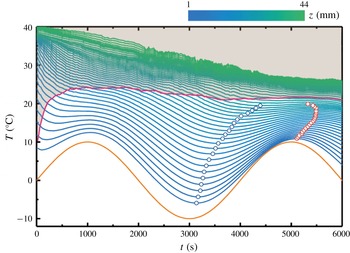
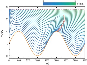
To further understand the growth of mushy layers under periodic cooling, it is helpful to examine the time-dependent temperature distribution within the mushy region. Figure 7 presents the mush temperature
 $T(z,t)$
as a function of time in the first two modulation periods
 $0\leqslant t\leqslant 2\unicode[STIX]{x1D70F}$
. These data are measured by an array of temperature probes with equal spacing of 1.0 mm over
 $1.0~\text{mm}\leqslant z\leqslant 23.0~\text{mm}$
(see detailed descriptions of the probe arrangements in § 2.2). The lowest curve shows the mush temperature
 $T_{1}(t)$
at a height
 $z=1.0~\text{mm}$
just above the bottom boundary. We see that
 $T_{1}(t)$
is forced to vary periodically with oscillating amplitude and phase similar to those of the bottom-plate temperature
 $T_{b}(t)$
(orange curve). However, in the first quarter modulation period
 $0\leqslant t\leqslant \unicode[STIX]{x1D70F}/4$
, the curve of
 $T_{1}(t)$
deviates significantly from a sinusoidal function due to initial transient cooling as the fluid temperature decreases rapidly from its initial value
 $T_{0}$
. After this transition time,
 $T_{1}(t)$
conforms to harmonic oscillations about
 $T_{b}(t)$
. Such a transition dynamics is notable for all temperature curves
 $T(z,t)$
at different heights within the mushy layer, after which they follow approximately periodic oscillations. The mush temperature increases monotonically with height within the layer.
The fluid temperature as a function of time at various heights measured in the first modulation period. The coloration represents the heights as indicated by the upper colour bar. The dashed curve shows the position of the mush–liquid interface and above that the liquid region is indicated in shadow colour. The orange curve shows the variation of the bottom temperature
 $T_{b}(t)$
. The minima of
 $T(z,t)$
in the first modulation period and the maxima in the second modulation period are marked by the blue and red circles, respectively. Experimental results for
 $A=10~\text{K}$
,
 $\unicode[STIX]{x1D70F}=4000~\text{s}$
and
 $\unicode[STIX]{x1D719}_{0}=0$
.

Numerical results for the fluid temperature distribution as a function of time within the mushy layer. The height is indicated by the colour scale. Results for
 $A=10~\text{K}$
,
 $\unicode[STIX]{x1D70F}=4000~\text{s}$
and
 $\unicode[STIX]{x1D719}_{0}=0$
. The minima of
 $T(z,t)$
in the first modulation period and the maxima in the second modulation period are marked by the blue and red circles, respectively. The orange curve shows the variation of the bottom temperature
 $T_{b}(t)$
.

The mush temperature
 $T(z,t)$
captured in figure 7 reveals another important feature: when the height increases, the oscillation amplitudes in
 $T(z,t)$
decrease, but the phase lag behind
 $T_{b}$
increases. We determine the oscillation phases of
 $T(z,t)$
through their local minima
 $T_{v}(z,t_{v})$
at a time
 $t_{v}$
immediately following
 $t\approx 3\unicode[STIX]{x1D70F}/4$
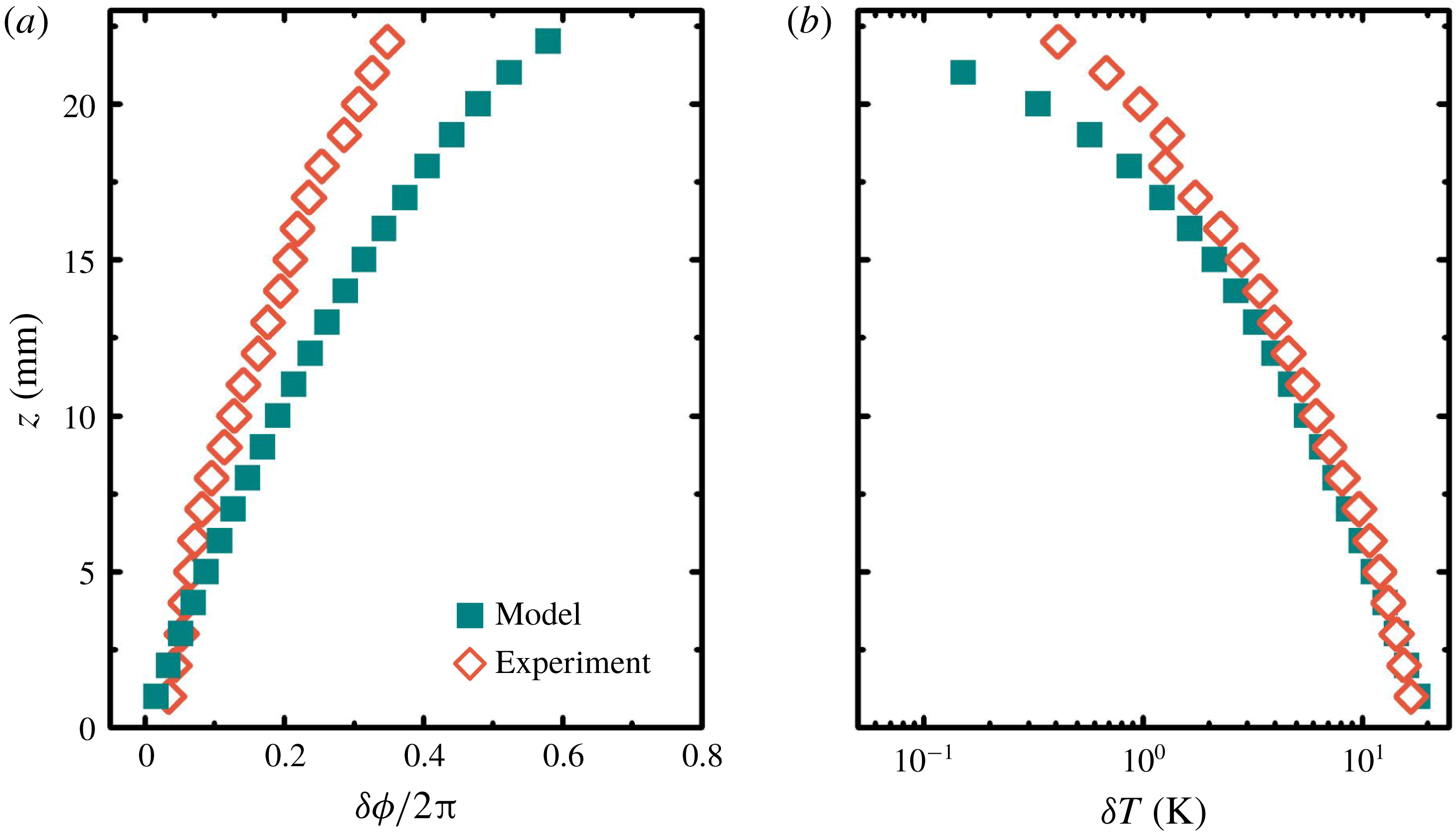
, as indicated by the open blue circles in figure 7. The phase lag of
 $T(z,t)$
behind
 $T_{b}$
,
 $\unicode[STIX]{x1D6FF}\unicode[STIX]{x1D719}=2\unicode[STIX]{x03C0}t_{v}/\unicode[STIX]{x1D70F}-3\unicode[STIX]{x03C0}/2$
, increases with increasing height as shown in figure 9(a). Also of interest is the time-dependent oscillation amplitude in
 $T(z,t)$
. With the second maxima in the temperature traces in figure 7,
 $T_{p}(z,t_{p})$
, we compute the temperature difference
 $\unicode[STIX]{x1D6FF}T=T_{p}-T_{v}$
. Results for
 $\unicode[STIX]{x1D6FF}T$
at different heights are presented in figure 9(b). They indicate that the oscillation amplitude
 $\unicode[STIX]{x1D6FF}T$
decreases with increasing height within the mush, and approaches zero near the mush–liquid interface.
The evolution of the mush temperature suggests that modulation of the bottom temperature
 $T_{b}$
generates temperature oscillations, or thermal waves that propagate from the bottom boundary towards the mush–liquid interface. The propagation of phase and decay of the oscillation amplitude with height are reminiscent of a classical thermal wave solution
 $T\sim T_{0}(z)+A\text{e}^{-z/\unicode[STIX]{x1D6FF}}\sin (\unicode[STIX]{x1D714}t+\unicode[STIX]{x1D719}-z/\unicode[STIX]{x1D6FF})$
for a constant-coefficient heat equation with a periodic modulation of the boundary temperature (Carslaw & Jaeger Reference Carslaw and Jaeger1959), where
 $T_{0}(z)$
is the steady background temperature. In this solution, the decay rate depends on the skin depth
 $\unicode[STIX]{x1D6FF}=\sqrt{\unicode[STIX]{x1D6FC}/\unicode[STIX]{x1D714}}$
which represents the characteristic length scale for diffusion of the thermal signal over a modulation period. The phase lag increases with height due to the diffusive time required for the propagation of the changing boundary temperature through the medium. In Part 2 (Ding et al.
Reference Ding, Wells and Zhong2019) we show that perturbations of this form can be justified for small-amplitude and high-frequency modulation with
 $\unicode[STIX]{x1D714}h^{2}/\unicode[STIX]{x1D6FC}\gg 1$
about the late-time steady state. However, in the present early-time limit the phase lag
 $\unicode[STIX]{x1D6FF}\unicode[STIX]{x1D719}$
shows some nonlinear variation with height and the amplitude
 $\unicode[STIX]{x1D6FF}T$
shows faster than exponential decay near the mush–liquid interface. This might be due to significant variation of the solid fraction
 $\unicode[STIX]{x1D719}(z,t)$
with time and height during early growth, leading to varying material properties. Alternatively, it may imply some non-trivial interaction of the thermal wave with the heat-flux balance of the mush–liquid interface. The propagation of thermal waves also provides further context on the amplitude decay and increasing phase lag of
 $\unicode[STIX]{x1D6FF}h$
seen over time in figures 4 and 5, due to the impact on the thermal gradient at the mush–liquid interface that controls mushy-layer growth. The amplitude of the thermal wave decays with height, whilst the time delay increases with height. These have corresponding impacts on the thermal gradient at
 $z=h$
as
 $h(t)$
increases over time. Hence the amplitude of
 $\unicode[STIX]{x1D6FF}h$
should decay over time and the phase lag should increase as the mushy layer gets thicker, consistent with figures 4 and 5.
Properties of oscillations of the temperature
 $T(z,t)$
as a function of height. (a) The phase lags of the minima of
 $T(z,t)$
in the first modulation period. (b) The peak-to-trough temperature amplitude
 $\unicode[STIX]{x1D6FF}T=T_{p}-T_{v}$
. Open diamonds: experimental data; solid squares: numerical data. Results extracted from the temperature traces shown in figures 7 and 8.

With the same reasoning we can understand the experimental result that the relative mushy-layer heights
 $|\unicode[STIX]{x1D6FF}h|$
are greater in a positive mode with
 $\unicode[STIX]{x1D719}_{0}=0$
than those in a negative mode
 $(\unicode[STIX]{x1D719}_{0}=\unicode[STIX]{x03C0})$
. In a positive mode the mushy layer grows slower due to a higher bottom-boundary temperature
 $T_{b}$
in the first half of the modulation period. The mushy-layer thickness
 $h(t)$
is on average less than that in a negative mode. Since the thermal wave has to propagate a shorter distance to reach the interface, the effect of the temperature oscillation is more pronounced at the mush–liquid interface in a positive mode, leading to a larger oscillation amplitude in
 $h(t)$
. Thus we observed troughs of
 $\unicode[STIX]{x1D6FF}h$
with greater amplitudes than the peaks in figures 3–5. We conclude that the thickness of the mushy layer has a significant influence on the dynamics of mushy-layer growth under periodic modulation due to the time taken for thermal changes to diffuse through the mushy layer.
In figure 8 we present the corresponding numerical results of the space–time distribution of the mush temperature
 $T(z,t)$
. Our numerical data replicate the main features of the variation of
 $T(z,t)$
observed in the experiment: the initial transient dynamics and the upward propagation of thermal oscillations through the mushy layer. The significant delay in the phase of the mush temperature
 $T(z,t)$
compared with
 $T_{b}$
is shown as a function of height in figure 9(a). Our numerical prediction of
 $\unicode[STIX]{x1D6FF}\unicode[STIX]{x1D719}$
increases slightly faster with height than the experimental results. This might be due to a lower solid fraction in the model than the observations, caused by neglecting solute fluxes from the mushy layer in the model. A lower solid fraction results in smaller thermal diffusivity (via lower conductivity
 $k_{m}$
and higher heat capacity
 $cp_{e}$
), a smaller value of
 $\unicode[STIX]{x1D6FF}=\sqrt{\unicode[STIX]{x1D6FC}/\unicode[STIX]{x1D714}}$
and increased phase lag due to the longer time taken for the thermal wave to propagate to a height
 $z$
. The model also overestimates the mean thickness
 $h(t)$
. The neglect of convection within the mushy layer also neglects the downward advective heat flux across most of the mush–liquid interface between the plumes from the chimneys. This may contribute to the observed overestimate of
 $h(t)$
in the model. We also note that the model predicts a larger liquidus temperature at the mush–liquid interface than observed, which is also consistent with neglect of solute fluxes and their impact on depletion of concentration in the liquid region in the experiment. However, it is curious that the modelled decay of the oscillation amplitudes in
 $T(z,t)$
is much closer to the experimental data in figure 9(b), with noticeable differences only near the mush–liquid interface.
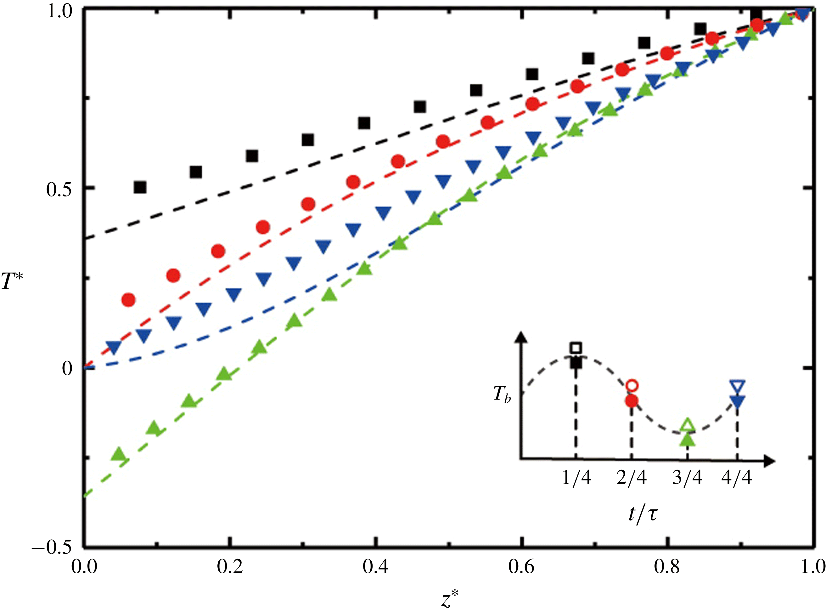
Four instantaneous profiles of normalized temperature
 $T^{\ast }(z^{\ast })=[T(t)-T_{b,0}]/[T_{i}(t)-T_{b,0}]$
of the mushy layer measured during the first modulation period, where
 $z^{\ast }=z/h(t)$
. Symbols: experimental data; dashed lines: numerical results. The inset sketches the variation of the bottom temperature in these four phases. Results for
 $A=10~\text{K}$
,
 $\unicode[STIX]{x1D70F}=4000~\text{s}$
and
 $\unicode[STIX]{x1D719}_{0}=0$
.

6.2 Comparison of experimental and numerical results for the time-dependent temperature profiles
For more direct comparisons with the experimental data, in figure 10 we present four instantaneous temperature profiles
 $T^{\ast }(z^{\ast })$
for the positive mode at evenly spaced time intervals within the first modulation period (
 $t=i/4\unicode[STIX]{x1D70F},i=1,2,3,4$
). These profiles are normalized both in height by the mushy-layer thickness
 $h(t)$
and in temperature by
 $T_{i}(t)-T_{b,0}$
, i.e.
 $z^{\ast }=z/h(t)$
and
 $T^{\ast }(t)=[T(t)-T_{b,0}]/[T_{i}(t)-T_{b,0}]$
. They imply that a periodic cooling boundary gives rise to temperature profiles with a mean slope
 $\langle \text{d}T^{\ast }/\text{d}z^{\ast }\rangle$
that varies periodically. In the phase with the lowest (or highest) bottom temperature
 $\langle \text{d}T^{\ast }/\text{d}z^{\ast }\rangle$
is maximum (or minimum). However, in the phases when
 $T_{b}=0.0\,^{\circ }\text{C}$
, the slope
 $\text{d}T^{\ast }/\text{d}z^{\ast }$
decreases with
 $z^{\ast }$
in the second phase (
 $i=2$
) when
 $T_{b}$
is decreasing in time; but increases with
 $z^{\ast }$
in the fourth phase (
 $i=4$
) when
 $T_{b}$
is increasing over time.
These profiles reveal an asymmetry of the mush temperature in time, because of the delays that occur when temperature oscillations propagate from the bottom plate towards the mush–liquid interface. For a constant-cooling mode, where the boundary temperature
 $T_{b}$
is held fixed, the mush-temperature distribution evolves according to
 $T_{eq}^{\ast }(z^{\ast },T_{b})=[T_{b}-T_{b,0}]/[T_{i}-T_{b,0}]+\text{erf}(az^{\ast })/\text{erf}(a)$
, with the parameter
 $a=Dcp_{m}\unicode[STIX]{x1D6EC}/k_{m}$
and the growth rate coefficient
 $\unicode[STIX]{x1D6EC}$
given by
 $h_{0}(t)=2\unicode[STIX]{x1D6EC}(Dt)^{1/2}$
(Huppert & Worster Reference Huppert and Worster1985). When
 $T_{b}$
is modulated periodically, however, due to the finite heat capacity within the mush domain, the phase lag of the local mush temperature behind
 $T_{b}$
increases with height. Such a delay is more pronounced in the phases with
 $T_{b}=0.0\,^{\circ }\text{C}$
(
 $i=2,4$
), when the temperature at the bottom varies most rapidly. In the phases when
 $T_{b}$
is increasing, the delay effect leads to a local mush temperature lower than
 $T_{eq}^{\ast }$
; curves of
 $T^{\ast }(z^{\ast })$
are concave and have an increasing slope when
 $z^{\ast }$
increases. On the contrary, in the phases when
 $T_{b}$
is decreasing, the delay effect causes a local mush temperature higher than
 $T_{eq}^{\ast }$
; curves of
 $T^{\ast }(z^{\ast })$
are all convex. When
 $T_{b}$
is close to a maximum or minimum, the variation of
 $T_{b}$
in time is relatively slow, allowing a longer time for the local mush temperatures to diffusively relax and approach closer to the vertical profile
 $T_{eq}^{\ast }(z^{\ast },T_{b})$
in the constant-cooling mode. In the first phase with
 $t/\unicode[STIX]{x1D70F}=1/4$
, since
 $T_{b}$
increases before it reaches a maximum, the local temperature in the interior of the mushy layer is still slightly lower than that in the constant-cooling mode and
 $T^{\ast }(z^{\ast })$
is more concave than
 $T_{eq}^{\ast }(z^{\ast },T_{b})$
. However, the error-function profile itself is convex, and the net effect is that
 $T^{\ast }(z^{\ast })$
appears close to a linear distribution in this period as shown by the black data curve in figure 10. In the third phase with
 $t/\unicode[STIX]{x1D70F}=3/4$
, however,
 $T_{b}$
decreases before it reaches a minimum, and the interior mush temperature is higher than that in the constant-cooling mode. We observed that the temperature profile at this time is convex. The predictions from the numerical model mostly coincide with our experimental data, with a slight tendency for the model to produce more curvature of
 $T^{\ast }(z^{\ast })$
.
According to the above discussions, the agreement between the experimental data and the numerical results in different aspects of the mushy-layer growth dynamics suggests that the present numerical model captures the key mechanisms that govern the early-time evolution of mushy layers with periodic cooling.
7 Discussions and concluding remarks
This paper presents comprehensive studies of the thickness and temperature distributions of a growing mushy layer when a binary aqueous solution is subject to periodic cooling from below. In the new experimental protocol, the temperature of the cooling boundary
 $T_{b}(t)$
is modulated to vary as a simple harmonic oscillation over time. The apparatus allows independent variations of the temperature modulation amplitude
 $A$
and frequency
 $\unicode[STIX]{x1D714}$
. We find that the mushy-layer growth is sensitive to the temperature variations. During modulation, the mushy-layer height
 $h(t)$
oscillates about the background growth
 $h_{0}(t)$
obtained for constant cooling. The oscillation amplitude of the relative height increases when the modulation amplitude increases, but decreases with an increasing modulation frequency. At very early times this is consistent with a scaling argument that predicts
 $h^{2}-h_{0}^{2}\propto A/\unicode[STIX]{x1D714}$
for quasi-steady modulation. However, the amplitude of the anomaly
 $h-h_{0}$
decays over time with accumulating phase lag.
We perform high-resolution measurements of the temperature distributions
 $T(z,t)$
within the mushy layer. The evolution of
 $T(z,t)$
can be interpreted in terms of propagating thermal waves that are generated due to the harmonic oscillations of the cooling temperature at the lower boundary. The experimental data reveal that when the mush height increases, the amplitudes of the temperature oscillations in the mush decay, and the phases of the oscillations increasingly lag behind
 $T_{b}$
. With these observations we provide fundamental explanations for the phase delays in the mushy-layer growth curve
 $h(t)$
and its asymmetry, with greater magnitudes of the peaks in a positive growth mode than the troughs in a negative mode.
Key features of these results are reproduced by a numerical model of mushy-layer growth with constant bulk concentration and subject to periodic modulation of the basal cooling across a range of modulation amplitudes and frequencies. The heat fluxes at the mush–liquid interface are parameterized by considering an overlaying liquid layer that undergoes vigorous convection, driven by a compositional gradient associated with finite solid fraction at the mush–liquid interface. The model yields one fitting parameter, which is chosen to capture the unmodulated growth at early times. The model is successful in replicating key features of the temperature distribution and evolution in the mushy layer, in terms of a decaying oscillation amplitude and an increasing phase lag of
 $T(z,t)$
with increasing height through the mushy layer. The numerical data predict time-dependent vertical temperature profiles where the slope increases (decreases) with height during modulation phases with increasing (decreasing) bottom temperature. This is broadly similar to the experimental observation, although the experiment shows less pronounced curvature.
Despite the good agreement between the theoretical model and the experiment, it is found that the model overestimates the mean thickness of the mushy layer. This is accompanied by greater phase lags in
 $T(z,t)$
than the experimental data, shown in figure 9(a). The experimental data also reveal a slightly faster decay of the oscillation amplitude of the relative mush thicknesses (figures 4 and 5). The present model neglects the rejection of relatively fresh water by convection from the interior of the mushy layer which has several effects. Neglecting the downward return flow of fluid from the mushy layer will underestimate the advective heat flux crossing the thermal boundary layer (Kerr et al.
Reference Kerr, Worster, Woods and Huppert1990b
), whilst a higher-concentration liquid layer is predicted which results in a higher liquid temperature at the interface and larger temperature differential during growth. These may give rise to faster growth and a thicker mushy layer in the numerical results than in the experiment. Furthermore, solute fluxes from the mushy layer would lead to increased internal solidification to maintain local thermodynamic equilibrium, and thus increased latent heat release in the mush interior in the experiment. This interior latent heat release would partially offset the cooling tendency at the mush–liquid interface, and thus slow mushy-layer growth in the experiment compared to the numerical solution. The convection flows present in the experiment may also cause a larger solid fraction, and thus increase the effective thermal diffusivity
 $\unicode[STIX]{x1D6FC}$
. This would lead to a larger decay length
 $\unicode[STIX]{x1D6FF}\propto \sqrt{\unicode[STIX]{x1D6FC}}$
and faster propagation speed of the temperature oscillations in the experiment than the numerical results (as seen in figure 9). Future developments of this modelling approach could incorporate the effects of solute rejection from the mush, include an explicit model of temperature and concentration fields in the liquid region and take into account the effects of heat leakage through the sidewalls of the sample due to imperfect thermal insulation of the apparatus. More insights may be obtained from the experimental side to investigate the evolution of the fluid concentration and temperature in the liquid region, to further parameterize the convection-driven heat and solute fluxes in the mushy layer and at the mush–liquid interface.
The results presented here may provide useful insight for environmental and engineering applications involving mushy-layer growth. For example, freezing of the polar oceans to form sea-ice involves the growth of a mushy layer with surface cooling that fluctuates due to atmospheric forcing. We expect such oscillations in surface temperature to drive thermal waves propagating through the depth of the mushy layer which decay towards the ice–ocean interface, inducing thickness changes as described above. Because the mushy layer is in local thermodynamic equilibrium, the temperature oscillations from the thermal wave induce corresponding changes in liquid concentration and solid fraction
 $\unicode[STIX]{x1D719}$
(the latter assuming that changes in bulk concentration are small over the time scale of the oscillation). Due to the decay of the thermal wave, we would hence expect to see larger-amplitude oscillations in
 $\unicode[STIX]{x1D719}$
near the cooling boundary. This may have implications for biogeochemical evolution and gas transport through sea-ice, which depends critically on the porosity
 $1-\unicode[STIX]{x1D719}$
of the ice matrix (Hunke et al.
Reference Hunke, Notz, Turner and Vancoppenolle2011). Such changes would simultaneously modulate the porosity-dependent permeability and gradients in the liquid concentration that control convective brine rejection from the ice (Notz & Worster Reference Notz and Worster2009). Varying porosity near the upper ice boundary also has implications for remote sensing techniques using scattering of electromagnetic waves (as discussed in Wettlaufer et al.
Reference Wettlaufer, Worster and Huppert2000).
The present work considers the evolution of the mush–liquid interface and the temperature distribution of a binary aqueous solution. During the initial modulation periods, the mushy layer undergoes rapid growth and its porosity structure and solid-fraction distribution evolve significantly in time. In Part 2 of this series of papers (Ding et al. Reference Ding, Wells and Zhong2019), we will extend our experimental studies and analysis to investigate the distribution of the mush temperature during late modulation periods when the fine mush structure becomes approximately time-independent. From this we determine the distribution of the solid fraction in mushy layers.
Acknowledgements
This work was supported by the National Science Foundation of China through grant nos 11572230 and 11772235, and NSFC/RGC Joint Grant no. 11561161004. J.-Q.Z. acknowledges support from the Fundamental Research Funds for the Central Universities (grant nos 22120180115 and 22120180280). G.-Y.D. was supported partially by NSFC/RGC Joint Grant no. CUHK437/15. A.J.W. acknowledges European Union Award PCIG13-GA-2013-618610 SEA-ICE-CFD, and thanks the Isaac Newton Institute for Mathematical Sciences for hospitality during the programme Mathematics of Sea Ice Phenomena (EPSRC grant EP/K032208/1).
Supplementary movie
A supplementary movie that shows the growth of mushy layers and the flow fields in the liquid region in three modulation modes (
 $\unicode[STIX]{x1D719}=0$
, constant cooling and
 $\unicode[STIX]{x1D719}=\unicode[STIX]{x03C0}$
) is available at https://doi.org/10.1017/jfm.2019.256.