



1. Introduction
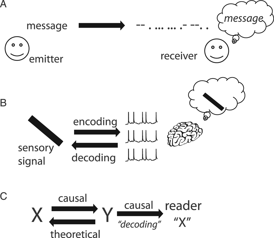
A pervasive paradigm in neuroscience is the concept of neural coding (deCharms and Zador Reference deCharms and Zador2000): the query “neural coding” on Google Scholar retrieved about 15,000 papers in the last 10 years. Neural coding is a communication metaphor. An example is the Morse code (Fig. 1A), which was used to transmit texts over telegraph lines: each letter is mapped to a binary sequence (dots and dashes). In analogy, visual signals are encoded into the spike trains of retinal ganglion cells (Fig. 1B). Both the Morse code and the retinal code relate to a communication problem: to communicate text messages over telegraph lines, or to communicate visual signals from the eye to the brain. This problem has been formalized by communication theory (Shannon Reference Shannon1948), also called information theory, a popular tool in neuroscience (Rieke et al. Reference Rieke, Warland, van Stevenick R. and Bialek1997).
The coding metaphor. (A) An emitter transmits a message to a receiver in an altered form called “code” (here the Morse code). The receiver knows the correspondence and can reconstruct (“decode”) the original message. (B) In analogy, visual signals are encoded in the spike trains of the optic nerve. The rest of the visual system treats these spike trains as visual information. (C) Implicit structure of the neural coding metaphor (“Y encodes X”). There is correspondence between X and Y. Encoding refers to a causal mechanism from X to Y, and decoding is a theoretical inverse mapping; Y causes changes in the reader (often improperly called “decoding”) and represents X in some sense.
The neural coding metaphor has shaped neuroscience thinking for more than five decades. Barlow (Reference Barlow and Rosenblith1961) used the metaphor extensively in his work on sensory neurons, although he warned to “not regard these ideas as moulds into which all experimental facts must be forced.” In a seminal review entitled Neural Coding, Perkel and Bullock (Reference Perkel and Bullock1968) depicted “the nervous system [as] a communication machine” and already recognized the “widespread use of “code” in neuroscience.” An illustration of hieroglyphs figures prominently at the top of the technical appendix. Around the same time, entire books were devoted to “sensory coding” (Somjen Reference Somjen1972; Uttal Reference Uttal1973).
As the linguists Lakoff and Johnson (Reference Lakoff and Johnson1980a) have argued, the metaphors that pervade our language are not neutral; on the contrary, they form the architecture of our conceptual system. What are the concepts carried by the neural coding metaphor that make it a possibly relevant metaphor for the activity of the retina? There are three key properties (Fig. 1C), which are all used in Perkel and Bullock's (Reference Perkel and Bullock1968) review:
1. The technical sense of a code is a correspondence between two domains, for example, visual signals and spike trains. We call this relation a code to mean that spike trains specify the visual signals, as in a cipher: one can theoretically reconstruct the original message (visual signals) from the encoded message (spike trains) with some accuracy, a process called decoding. Information theory focuses on statistical aspects of this correspondence (Shannon Reference Shannon1948). It is in this sense that neurons in the primary visual cortex encode the orientation of bars in their firing rate, neurons in the auditory brainstem encode the spatial position of sounds (Ashida and Carr Reference Ashida and Carr2011), and neurons in the hippocampus encode the animal's location (Moser et al. Reference Moser, Kropff and Moser2008).
2. Yet, not all cases of correlations in nature are considered instances of coding. Climate scientists, for example, rarely ask how rain encodes atmospheric pressure. Another key element of the coding metaphor is that the spike trains are considered messages for a reader, the brain, about the original message: this is the representational sense of the metaphor. Perkel and Bullock call the reader's activity “interpretation of the encoded information.” In his book on sensory coding, Somjen (Reference Somjen1972) writes: “Information that has been coded must at some point be decoded also; one suspects, then, that somewhere within the nervous system there is another interface … where ‘code’ becomes ‘image.’” Similar statements abound in modern neuroscience literature: “A stimulus activates a population of neurons in various areas of the brain. To guide behavior, the brain must correctly decode this population response and extract the sensory information as reliably as possible” (Jazayeri and Movshon Reference Jazayeri and Movshon2006).
3. Finally, we would not say that visual signals encode retinal spike trains, even though this would comply with the technical sense. The reason is that the communication metaphor implicitly assumes a causal relation between the original message and the encoded message; here, spike trains result from visual signals by a causal process (transduction). Similarly, to be a representation for a reader, the neural code must at least have a causal effect on the reader. This causal structure is implicit in Perkel and Bullock's (Reference Perkel and Bullock1968) definition of neural coding: “the transformations of information in the nervous system, from receptors through internuncials to motor neurons to effectors.”
These three elements (correspondence, representation, causality) constitute the conceptual scaffold of the neural coding metaphor. It could be argued that most technical work on neural coding uses only the first technical sense (correspondence), where the word code is used as a synonym for correlate. The use of the metaphor would thus amount to only an inappropriate but innocuous choice of words. But what is the scope of neural codes if they have no causal powers? In his famous critique of Skinner's behaviorism, Chomsky et al. (Reference Chomsky1959) summarizes the problem with the improper use of metaphors: “[Skinner] utilizes the experimental results as evidence for the scientific character of his system of behavior, and analogic guesses (formulated in terms of a metaphoric extension of the technical vocabulary of the laboratory) as evidence for its scope.” The goal of this article is to demonstrate that this quote fully applies to the neural coding metaphor, where “scope” is a particular theory of brain function implied by the conceptual structure of the metaphor.
The general argument is as follows. Scientific claims based on neural coding rely on the representational sense or at least on the causal sense of the metaphor. But none of these two senses is implied by the technical sense (correspondence). When we examine the representational power of neural codes (part 1), we realize that coding variables are shown to correlate with stimulus properties but the code depends on the experimental context (stimulus properties, protocol, etc.). Therefore, neural codes do not provide context-free symbols. But context cannot be provided by extending the code to represent a larger set of properties, because context is what defines properties (e.g., the orientation of a bar). Thus, neural codes have little representational power. The fundamental reason (part 2) is that the coding metaphor conveys an inappropriate concept of information and representation (Bickhard Reference Bickhard2009; Bickhard and Terveen Reference Bickhard and Terveen1996). Neural codes carry information by reference to things with known meaning. In contrast, perceptual systems have no other option than to build information from relations between sensory signals and actions, forming a structured internal model. Finally (part 3), the neural coding metaphor tries to fit the causal structure of the brain (dynamic, circular, distributed) into the causal structure of neural codes (atemporal, linear), substituting the arbitrary temporality of algorithms for the temporality of the underlying physical system. The two causal structures are incongruent. Without denying the usefulness of information theory as a technical tool, I conclude that the neural coding metaphor cannot constitute a valid basis for theories of brain function because it is disconnected from the causal structure of the brain and incompatible with the representational requirements of cognition.
2. Encoding stimulus properties
2.1. Encoding an experimental parameter
The activity of neurons is often said to encode properties, for example, “Many cortical neurons encode variables in the external world via bell-shaped tuning curves” (Seriès et al. Reference Seriès, Latham and Pouget2004). Here the authors refer to a particular type of experiment, where a parameterized stimulus is presented to an animal and the activity of a neuron is recorded. For example, the orientation of a small bar is varied and the activity of a neuron in the primary visual cortex is recorded (Fig. 1B). It is found that orientation and neural activity co-vary and, hence, the neuron's firing rate encodes the orientation of the bar in the sense of correspondence. What is the scope of such a proposition?
I will discuss a cartoon example from color perception, used by Francis Crick to warn against the “fallacy of the overwise neuron” (Crick Reference Crick1979). Cones are broadly tuned to wavelength (Schnapf et al. Reference Schnapf, Kraft and Baylor1987); in an experiment where light of different wavelengths is flashed, the amplitude of the transduced current varies systematically with wavelength (Fig. 2A). Thus, the current encodes wavelength in the technical sense of correspondence; one can recover wavelength from the magnitude of the current. Yet animals or humans with a single functional type of cone are color blind. Why are they color blind if their cones encode color information? This is clear in Figure 2A; if the current also depends on light intensity, then it does not provide unambiguous information about wavelength. In other words, the cone does not in fact encode wavelength in any general setting, even in the narrow sense of correspondence. The same remark applies to any tuning curve experiment.
Encoding wavelength of light. (A) Response of a cone to flashed light as a function of wavelength (cartoon), at different intensities (grays). If intensity is fixed, wavelength can be inferred from transduced current. Otherwise, current is not informative about wavelength. (B) In a tuning curve experiment, the coding relation is implied by the experimental design: wavelength is mapped to stimulus, which is transduced into current. (C) If wavelength is only one property of a larger set of stimuli, there might be no coding relation. (D) The relative response of cones with different tunings may provide intensity-invariant information about wavelength.

Formally, the logical problem can be analyzed as follows. The tuning curve experiment shows a correspondence between stimulus parameter and current. This correspondence is composed of two parts (Fig. 2B): a mapping from wavelength to stimulus, which is experiment specific, and the transduction of stimulus into current. Thus, the experimental design ensures that there exists a mapping from wavelength to current. In other words, the proposition that the neuron encodes the experimental parameter is mainly a property of the experimental design rather than a property of the neuron (which only needs to be sensitive to the parameter). However, the situation is completely different in the real world, which is not constrained by the experimental design (Fig. 2C). In general, there might be a variety of stimuli, one of their properties being wavelength. In this case, there is a mapping from stimulus to wavelength and a mapping from stimulus to current, and it is not obvious at all that there is a mapping from wavelength to current, because current depends also on other properties. In this context, the proposition that the neuron encodes wavelength is a much stronger claim, but it is not at all entailed by the tuning curve experiment.Footnote 1 This confusion underlies influential neural coding theories of perception, for example, Bayesian theories (Jazayeri and Movshon Reference Jazayeri and Movshon2006; Pouget et al. Reference Pouget, Dayan and Zemel2003), in which a neuron's firing rate is assumed to be a function of the stimulus parameter, rather than a context-dependent correlate (see sect. 2.3.2).
Thus, the correct interpretation of the tuning curve experiment is that the neuron is sensitive to the stimulus parameter, while to encode a property of stimuli (a “variable in the external world”) is a somewhat orthogonal proposition; it means that the observable is not sensitive to other properties. For example, a color scientist would point out that wavelength is indeed not encoded by single cones, but by the relative activity of cones with different tunings (Fig. 2D), because that quantity does not depend on light intensity. Thus, referring to tuning curve experiments in terms of coding promotes a semantic drift, from the modest claim that a neuron is sensitive to some experimental manipulation to a much stronger claim about the intrinsic representational content of the neuron's activity. We will now see that this semantic drift indeed operates in current theories of brain function.
2.2. The overwise neuron and its ideal observer
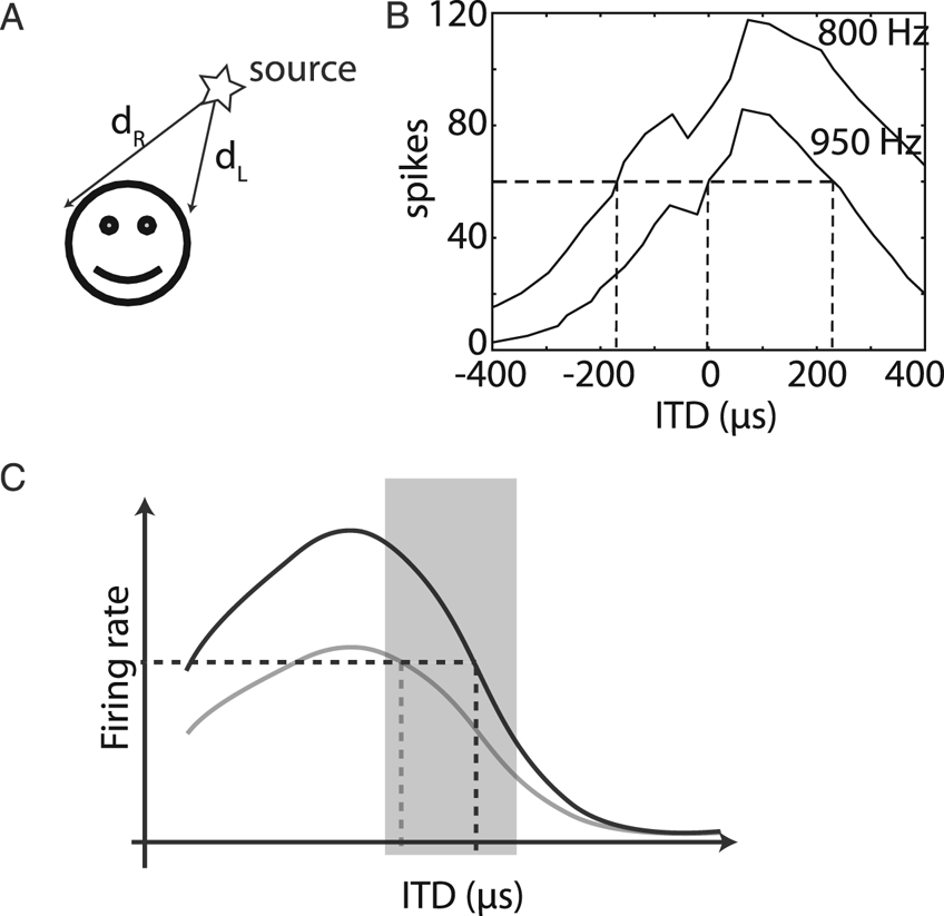
To understand how the neural coding metaphor unfolds, I will discuss one particular example in detail (but another one could have been chosen). In mammals, the major cue for sound localization in the horizontal plane is the difference in arrival times of the sound wave at the two ears (interaural time difference [ITD]) (Fig. 3A). Neurons in the medial superior olive (MSO) (in the auditory brainstem) are sensitive to this cue (Joris et al. Reference Joris, Smith and Yin1998); when a sound is played through earphones and the ITD is varied, the firing rate of those neurons changes (Fig. 3B). These neurons project to neurons in the inferior colliculus (IC), which also have diverse ITD tuning properties. Electrical stimulation in the cat's IC triggers an orienting response toward a particular contralateral direction, with stronger stimulations resulting in responses with a larger part of the body (one pinna, both pinnae, and eyes), by a pathway involving the superior colliculus (Syka and Straschill Reference Syka and Straschill1970). Unilateral lesions in the MSO or IC result in sound localization deficits in the contralateral field (Jenkins and Masterton Reference Jenkins and Masterton1982). Therefore, neurons in the IC have a critical role in localizing sounds in the contralateral field.
Encoding sound location. (A) A major cue for sound localization is the interaural time difference (ITD), d R – d L. (B) Number of spikes in response to two binaural tones (950 and 800 Hz) as a function of ITD for the same neuron in the medial superior olive of a cat (digitized from Yin and Chan [Reference Yin and Chan1990], Fig. 10). It is possible to infer the ITD from spike count if the experimental configuration (presented tone) is known, not if the sound is a priori unknown. (C) If the organism lived in a world with a single sound played at different ITDs, then the best way to encode ITD would be with a neuron tuned to an ITD outside the range of natural sounds (shaded), so that the selectivity curve is steep inside that range. However, the response of a single neuron is fundamentally ambiguous when sounds are diverse, irrespective of the steepness of the curve (selectivity curve for another sound shown in gray).
How does the activity of these neurons contribute to sound localization behavior? One way is consider the entire pathway, try to build a model of how neuron responses in various structures combine to produce an orientation reflex to a localized sound, and compare with the diverse experimental observations mentioned above. Another way is to ask how neurons encode sound location (McAlpine et al. Reference McAlpine, Jiang and Palmer2001). It has, for example, been claimed that “there is sufficient information in the firing rates of individual neurons to produce ITD just-noticeable-differences that are comparable with those of humans psychophysically” (Shackleton et al. Reference Shackleton, Skottun, Arnott and Palmer2003, p. 723; Skottun Reference Skottun1998). What does this mean, and how significant is this fact?
The neuron of Figure 3B encodes ITD in the technical sense that one can estimate the ITD with some accuracy from the observation of the number of spikes, by inverting the tuning curve (i.e., decoding the neuron's response). It turns out that this accuracy is similar to the accuracy of sound localization by the animal. But the neuron's response is also sensitive to various aspects of sound (e.g., frequency, intensity), so our decoder would give totally inaccurate results in any other context. Therefore, the performance of this decoder is unrelated to our general ability to localize sounds. Yet, although the problem of ambiguities was acknowledged, it was concluded that “it might not be necessary to pool the outputs from many neurons to account for the high accuracy with which human observers can localize sounds” (Skottun Reference Skottun1998). This conclusion is unwarranted because tuning curves address the exactly orthogonal problem (sensitivity to ITD vs. insensitivity to other dimensions).
This incorrect conclusion is about localization, but what about discrimination? The first quote compared the tuning curve to discrimination performance, that is, psychophysical measurements of the ability to discriminate between two sounds that differ only by their ITD. This is a more restricted situation, but how can the responses of a single neuron be compared with the behavior of an organism without making any reference to the mechanisms that might link this neuron's activity to behavior (e.g., the pathway mentioned earlier)? More generally, how can a neural code be about behavior, when it is technically only about stimulus-response properties? This requires what Teller (Reference Teller1984) called a “linking proposition,” an implicit postulate that directly relates neural activity to behavior. The linking proposition here, as in many neural coding studies, is that the brain implements an “ideal observer” (Macmillan and Creelman Reference Macmillan and Creelman2005). This is the representational sense of the metaphor, namely, the idea that neural responses are messages for a reader. The empirical question, then, is how plausible is this linking proposition?
Let us spell it out. The ideal observer reads the activity of the neuron. When the first stimulus is presented, it stores the number of spikes produced by the neuron in a window of a given duration (chosen by the experimenter) after the stimulus. It ignores all spikes produced before and after that window until the second stimulus is presented, upon which it stores again the number of spikes produced by the neuron. Then it retrieves the two stored numbers, compares them (and not others, e.g., the activity of other neurons), and decides to push one of two buttons. It is not so obvious how this ideal observer can be mapped to the pathway described above, for example, how the number of spikes of an arbitrary neuron in the brainstem, produced during several predefined time windows, can be stored in working memory for later comparison.
The ideal observer is ideal in the sense that it makes the best use of all available information. This includes the neural activity itself, but most importantly all the information that is available to the experimenter: when exactly the activity corresponds to the stimulus, what stimulus has been presented, the knowledge that the exact same sounds are played twice, which parts of the activity should be stored. On the other hand, the observer is not ideal in the sense that it uses nothing more than the information available to the experimenter. For example, if it also used the information available in other neurons (not recorded), then discrimination performance would be much better than psychophysical measurements. In other words, the ideal observer is not the best thing that the brain can do; it is the best thing that the experimenter can do.
Thus, by implying that the brain reads the neural code, we manage to make claims about perception and behavior while totally ignoring the mechanisms by which behavior is produced, as well as the constraints that the organism must face in ecological situations (e.g., not knowing the sound presentation protocol in advance). These claims rely on implicit linking propositions based on abstract constructs, where neural activity is likened to a processor register that the brain manages to store, retrieve, and manipulate, wherever it is in the brain and whenever it occurs. It would seem that empirical evidence or argumentation should be required to support such questionable hypotheses, since all conclusions are based on them. Why is it that no such justification is ever provided when “ideal observers” are introduced? The reason, it seems, is the semantic drift from the technical sense of code to the representational sense of code, which is logically flawed. The same flaw appears to underlie leading theories of neural population coding.
2.3. Populations of overwise neurons
2.3.1. Slope coding
What is the optimal way to encode ITD in the activity of neural populations? If all confounding dimensions (level, frequency, etc.) are neglected, then the best way to encode ITD is to have a steep monotonous relation between ITD and firing rate, that is, to maximize neural sensitivity to the ITD (Fig. 3C). Thus, the neuron's preferred ITD should lie outside the range of natural sounds (around ±800 μs for humans [Benichoux et al. Reference Benichoux, Rébillat and Brette2016]) while the steepest slope of the selectivity curve should be inside. This is the concept of “slope coding.” Thus, it has been argued that the optimal way to encode ITD is with two homogeneous populations of neurons with symmetrical tuning curves, peaking at ITDs that are not normally experienced (Harper and McAlpine Reference Harper and McAlpine2004). Unfortunately, this conclusion is based entirely on the fallacy of the overwise neuron. If confounding dimensions are not neglected, then the opposite conclusion follows: As in the case of cones, heterogeneity of ITD tunings is crucial to resolve the ambiguities resulting from nonspatial dimensions of sounds (Brette Reference Brette2010; Goodman et al. Reference Goodman, Benichoux and Brette2013).
On the basis of the slope coding idea, a leading theory of sound localization (Grothe et al. Reference Grothe, Pecka and McAlpine2010) proposes that sound location is encoded in the relative average activity of the two populations of neurons. It was initially meant to explain why many neurons are tuned to large ITDs that are not normally experiencedFootnote 2 (McAlpine et al. Reference McAlpine, Jiang and Palmer2001). Although using the relative activity of two populations somewhat reduces the ambiguity resulting from sound level, the fact that sounds have more than two dimensions again means that this model is unlikely to work in practice unless the auditory world consists of pure tones (Goodman et al. Reference Goodman, Benichoux and Brette2013). In any case, what needs to be demonstrated to support this theory is not that tuning curves have a steep slope, but that the relative average activity of the two neural populations is insensitive to properties other than the ITD (e.g., the sound at the source). Thus, the application of the coding metaphor to tuning curve experiments leads to confusion between parameter sensitivity and information about the corresponding property in a broader context. It could be argued that information in a broad context at least requires sensitivity, but this is also technically incorrectFootnote 3 (see, e.g., Zylberberg Reference Zylberberg2018).
2.3.2. Encoding visual stimuli
In visual neuroscience, theories of neural coding are based on heterogeneous tunings. There are several theories of population coding of stimulus properties in the visual cortex (Jazayeri and Movshon Reference Jazayeri and Movshon2006; Pouget et al. Reference Pouget, Dayan and Zemel2003). One influential theory, the “Bayesian brain” hypothesis (Knill and Pouget Reference Knill and Pouget2004), postulates that neural activity represents the probability distribution of the stimulus property, which the brain can manipulate to perform statistical inference. A key assumption in this and other coding theories is that the firing rate of neurons is a context-free function of stimulus properties. This assumption appears explicitly in the models and in the way the brain is proposed to compute with those representations. For example, one variation of this theory proposes that the brain computes the log likelihood of a stimulus property by summing the activity of neurons weighted by the logarithm of each neuron's tuning curve (Jazayeri and Movshon Reference Jazayeri and Movshon2006). This operation is described as a “simple neural readout strategy,” because it involves only summation and multiplication by fixed weights. As already discussed, the problem is that in reality, tuning curves are defined for a specific experimental condition; they are not context free. Therefore, either the computation of the log likelihood will be systematically incorrect for all other conditions, or the weights used in the readout must be adapted to correspond to the tuning curve of each condition by an undescribed mechanism, in which case the readout cannot possibly be described as a “simple neural readout.”
To what extent do tuning curves depend on context? As it turns out, to a large extent. It has long been known that properties of sensory neurons adapt to input statistics (Barlow et al. Reference Barlow, Fitzhugh and Kuffler1957; Hosoya et al. Reference Hosoya, Baccus and Meister2005). In the primary visual cortex, responses to local orientation depend on the surrounding context (Bolz and Gilbert Reference Bolz and Gilbert1986; Hubel and Wiesel Reference Hubel and Wiesel1968). Tuning properties of visual cortical neurons (not just the gain) depend on cognitive context, including the task the animal is doing (Gilbert and Li Reference Gilbert and Li2013), locomotion (Pakan et al. Reference Pakan, Francioni and Rochefort2018), and prior presentation of sounds (Chanauria et al. Reference Chanauria, Bharmauria, Bachatene, Cattan, Rouat and Molotchnikoff2018). Current evidence indicates that the activity of neurons is sensitive to stimulus properties (the technical sense of coding) but cannot be considered as context-free symbols that stand for the corresponding properties (the representational sense of coding). Can neural coding theories of perception accommodate for this fact? It would require that in every context, changes in encoding (stimulus-response properties) are mirrored exactly by changes in decoding (computations performed on neural activity, e.g., the “simple neural readout”). No mechanism has been proposed to achieve this (see also next section).
Theories of neural coding have the ambition to explain some aspects of perceptual behavior, namely, results of psychophysical experiments. Again, this requires that a link is made between the neural code and behavior. This link involves ideal observers; for each possible task there is an optimal way to decode neural activity into the variable of interest, which uses detailed elements of the experimental design. Critically, this link with behavior is not considered part of the model because it is assumed that it belongs to the reader of the neural codes.Footnote 4 Thus, the behavioral predictions of the coding theories critically rely on linking propositions whose validity or plausibility is not addressed. To be clear, the questionable assumption is not so much whether behavior or perception is optimal in some way (Rahnev and Denison Reference Rahnev and Denison2018), but whether the activity of a neuron is something that is read and manipulated as if it were a register of a processor and not simply something that the neuron is doing at a particular time (acting on other neurons).
When the brain is engaged in solving a particular visual task, the activity of neurons depends specifically on object properties relevant to that task (Gilbert and Li Reference Gilbert and Li2013). This seems entirely logical if we see neurons as collaborating to solve a task. In contrast, it is surprising if we see the visual cortex as encoding the world and the remainder of the brain as dealing with this representation to guide actions. Thus, thinking in terms of coding seems to obscure rather than clarify understanding.
2.4. Can neurons encode variables?
It could be objected that the problem of contextual dependence of tuning curves calls only for a minor amendment to the mainstream neural coding theories, which is to consider that contextual variables are encoded too. This would require more complicated decoding schemes, but not fundamentally different theories.
For example, it could be proposed that populations of cones jointly encode wavelength and intensity, and both can be decoded from the joint activity of cones. But to decode cone activity into wavelength, it must be known that a monochromatic light is being presented. In natural experience, light is not monochromatic; it has a continuous spectrum, and the transduced current depends on the convolution of the spectrum of incident light with the absorption spectrum of the photoreceptor. In those cases, cones cannot possibly encode wavelength, even jointly, because there is no such thing as the wavelength of a patch of visual scene. Thus, the activity of cones is not sufficient to infer wavelength. A critical element of context that also needs to be encoded is the fact that a monochromatic light is being presented.
Similarly, a cat's neuron may encode the orientation of a bar only in conjunction with the information that a bar is being presented. That information does not take the form of a variable, but perhaps of a model of the experiment. But models are not variables; rather, they define variables. Thus, a perceptual scene cannot be represented by a set of variables, because this leaves out what defines variables. This missing aspect corresponds to object formation and scene analysis, two fundamental aspects of perception that are not addressed by coding: There is no object property to be encoded if there is no object.
Consider the Bayesian brain hypothesis: “the brain represents information probabilistically, by coding and computing with probability density functions” (Knill and Pouget Reference Knill and Pouget2004). This presupposes that there is a set of predefined variables to which probability is attributed – examples of variables are the position of an object and the orientation of a visual grating. If neurons encode variables, then what encodes the definitions of those variables, and what do neurons encode in situations where those variables are not defined? We can imagine that such theories might apply to the representation of eye position, for example, because the eye is always there and its position is always defined. This is not the case of objects of perception in general.
Similarly, influential models of working memory propose that memory items are stored and encoded in the persistent activity of neurons tuned to the underlying stimulus property, for example, the spatial position of an object (Constantinidis and Klingberg Reference Constantinidis and Klingberg2016). This provides a way to store graded properties, such as the position of a visual target or the pitch of a musical note. But suppose there is a neural network in my brain that is storing the number 100. What have I memorized? Clearly not the same piece of information if this number is the area of my apartment in square meters or the height of my son in centimeters. To store the information, one needs not only the number but also what it refers to. Can the persistent activity of tuned neurons store that information? It can if there is a network of neurons tuned to the area of my apartment and another tuned to the height of my son.
Perception and memory cannot just be about encoding stimulus properties because this omits the definitions of those properties and of the objects to which they are attached. But could it be that neurons encode more abstract “internal variables” that somehow describe the external world? Such is the claim of predictive coding (Rao and Ballard Reference Rao and Ballard1999) and related propositions such as the free energy principle (Clark Reference Clark2013; Friston Reference Friston2009). In these theories, neural coding is described as a statistical inference process, where neurons encode the inferred value of internal variables of a generative model of the inputs, for example, the retinal image. Technically, this essentially means that the code is a parametric description of the image (e.g., a Fourier transform). Described at this technical level, the theory seems to have little to say about perception or behavior. But the intended scope extends as these internal variables are described as the “causes” of the sensory input, and the process of encoding is referred to as “inferring the hidden causes.” The sensory input is caused by things in the world, so an internal variable can be considered a cause only if it is assumed to encode properties of objects in the world as in the Bayesian brain hypothesis. Again, this is incoherent because no perceptual scene can be fully specified by the properties of its objects; one needs first to define objects and their properties, and these definitions are not conveyed by the variables. “Cause” must then be understood in the strict technical sense of variable of a statistical function, which has little to do with the usual sense of “cause.” Thus, this use of the term cause appears to be another case of a metaphoric extension of the technical vocabulary. As Chomsky (Reference Chomsky1959, p. 30) observed, “This creates the illusion of a rigorous scientific theory with a very broad scope, although in fact the terms … [have] at most a vague similarity of meaning.” We will return to predictive coding theory in the next section.
Neurons encode stimulus properties according to the technical sense of the metaphor. To acquire a broad scope, the metaphor drifts into the representational sense, according to which neurons convey information about the said properties to the rest of the brain. But neural activity can only be interpreted as properties once the interpretative framework is provided. Critically, this framework is not contained in the coding variables. In what sense do neural codes constitute information for the brain if their meaning lies outside the encoded messages and varies depending on situations? Where do ideal observers obtain the information necessary to decode the messages? In the next section, I argue that the coding metaphor conveys a very particular notion of information, which is information by reference, and that this is not the kind of information relevant to perception and behavior.
3. Do neural codes constitute information about the world?
3.1. Codes as information by reference
The coding metaphor assumes that neural codes represent information about the world, which the brain uses to produce adapted behavior. This sense is implied by the use of ideal observers in the neural coding literature and, more generally, by the presumption that the brain “decodes” neural responses or “extracts information” from them. In what sense is the neural code “information” about objective properties of the world? According to the technical sense of coding, it is information in the sense that these properties can be inferred from neural activity. Methodologically, this inference is made by the experimenter, who confronts these properties with measurements of neural activity. But by using the term neural code and by comparing the output of ideal observers with psychophysical measurements, we imply that the brain must also make this inference.
This raises the issue of “the view from inside the box” (Clark Reference Clark2013): How is it possible for the nervous system to infer external properties from neural activity if all that it ever gets to observe is that activity? In fact, what does it even mean that a neural network infers external properties (e.g., the direction of a sound source), given that those properties do not belong to the domain of neural activity? This is related to the symbol grounding problem (Harnad Reference Harnad1990b): How do spikes, the symbols of the neural code, make sense for the organism?
A fundamental issue with the coding metaphor, as it applies to the brain, is that it conveys a very particular notion of information, information by reference; the meaning of the encoded message is that of the original message to which it refers. Shannon (Reference Shannon1948, p. 379) made this very clear when he defined his mathematical notion of information:
The fundamental problem of communication is that of reproducing at one point either exactly or approximately a message selected at another point. Frequently the messages have meaning; that is, they refer to or are correlated according to some system with certain physical or conceptual entities. These semantic aspects of communication are irrelevant to the engineering problem.
But the semantic aspects are precisely what is relevant to the biological problem: How does the brain know what the codes refer to?
One possibility is that the meaning of neural codes is implicit in the structure of the brain that reads them; the brain understands neural codes because it has evolved to do so. There are at least two objections that make this proposition implausible. First, there is considerable plasticity, including developmental plasticity, both in the nervous system and in the body, which makes the idea of a fixed code implausible. An impressive example is the case of a patient born with a single brain hemisphere, who has normal vision in both hemifields, with a complete reorganization of brain structure (Muckli et al. Reference Muckli, Naumer and Singer2009). This plasticity implies that the “reader” of neural codes must learn their meaning, at least to some extent. Second, it might be imagined that the meaning of a neural code for eye position might be fixed by evolution – that there are fixed motor circuits that control the eye based on that fixed neural code. But how could this be true of a neural code for the memory item “my apartment is 100 meters square”?
To see that Shannon information cannot be the notion of information relevant to understanding perception, consider the following experiment of thought, which I call the paradox of efficient coding. Suppose that all information about the world (including efferent copies) is encoded by a set of neurons. From the heuristic that biological organisms tend to be efficient, we now postulate that neurons transform their inputs in such a way as to transmit the maximum amount of information about the world, in the sense of Shannon; this is the efficient coding hypothesis (Barlow Reference Barlow and Rosenblith1961; Olshausen and Field Reference Olshausen and Field2004). This means that all redundancy is removed from the original signals. If it is done perfectly, then encoded messages are indistinguishable from random by the organism. Therefore, the perfectly efficient code cannot be understood by its reader.
It is indeed paradoxical that when we maximize the amount of information carried by code, we find something that provides no information at all to the reader. This is because the notion of information implied by the phrase “neurons encode information” is information by reference to the inputs, a kind of information that is accessible only to an external observer. This is not the right way to address the representational problems faced by the organism. As Bickhard has argued (Bickhard Reference Bickhard2009; Bickhard and Terveen Reference Bickhard and Terveen1996), “encodingism” fails to provide an adequate notion of representation because it does not allow the possibility of system detectable error; there is no way for the system to know whether the representation is in error.
Again, the coding metaphor appears to promote a semantic drift, from the technical sense of information as defined by Shannon to a broader sense of information that might be useful for an organism. The neural coding metaphor is so prevalent in the neuroscience literature that the notion of information it carries seems to be the only possible one: “the abstract definition of information is well motivated, unique, and most certainly relevant to the brain” (Simoncelli Reference Simoncelli2003, p. 145). Next, I discuss alternative notions of information that are more relevant to the brain.
3.2. Information as subjective laws or internal models
How can there be any information about the world without direct access to the world? John Eccles, a prominent neurophysiologist, expressed the problem in the following terms (Eccles Reference Eccles1965, p. 322):
In response to sensory stimulation, I experience a private perceptual world which must be regarded, neurophysiologically, as an interpretation of specific events in my brain. Hence I am confronted by the problem: how can these diverse cerebral patterns of activity give me valid pictures of the external world?
To him, the logical solution was a form of dualism, much like Cartesian dualism, except he did not believe that the interaction between mind and brain occurred at a single place (Descartes’ pineal gland). Dualism is a natural solution if neural activity is thought to encode information by reference to the external world, because the external world belongs to a different domain.
A number of philosophers and psychologists have proposed alternative solutions. O'Regan and Noë (Reference O'Regan and Noë2001) proposed the analogy of the “villainous monster.” Imagine you are exploring the sea with an underwater vessel. A villainous monster mixes all the cables; hence, all the sensors and actuators are now related to the external world in a new way. How can you know anything about the world? The only way is to analyze the structure of sensor data and their relationships to actions that you can perform. If dualism is rejected, then this is the kind of information that is available to the nervous system. A salient feature of this notion of information is that, in contrast to Shannon's information, it is defined as relations or logical propositions: If I do action A, then sensory property B occurs; if sensory property A occurs, then another property B occurs next; if I do action A in sensory context B, then C occurs.
Gibson (Reference Gibson1979) previously developed a related psychological theory. While criticizing the information-processing view of perception, he argued that there is information about the world present in the invariant structure of sensory signals: “A great many properties of the [optical] array are lawfully or regularly variant with change of observation point, and this means that in each case a property defined by the law is invariant.” Clearly, he did not mean information in the sense of communication theory, but rather in the sense of scientific knowledge. A set of observations and experiments provide information about the world in the form of laws that relate observables (sensory signals) between them and with possible actions. This form of information is intrinsic; I proposed calling this set of laws the subjective physics of the world (Brette Reference Brette and El Hady2016), which is related to von Uexküll's (Reference von Uexküll1909) Umwelt. A related view, formalized by theoretical biologist Robert Rosen (Reference Rosen1985), is that biological organisms build an internal model of the world in which the variables are sensory signals. This view addresses the symbol grounding problem by mapping sensory signals to elements of an internal model. The signals make sense in reference to that model; they are not mapped to externally defined properties. In Bickhard's (Reference Bickhard2009; Reference Bickhard2015c) interactivist model, representations are based on anticipatory relations between internal processes.
Crucially, relations between observables are precisely what neural coding theory considers as redundancy, which ideally should be eliminated. In contrast, in the alternative view discussed here, relations constitute information. This point was made by Thompson (Reference Thompson1968, p. 305). “It is our subjective habit to organize the individual elements of our experience, to cross-correlate these elements to others distant in space and time, and it is only after this process of imposing organization that we feel informed.” The number 100 does not really constitute information; only when I have inserted it into my internal model of the world by saying that it is the area of my apartment in square meters does it become information.
3.3. Subjective physics of the Martian iguana
To make this point more concrete, I will discuss an example adapted from Brette (Reference Brette and El Hady2016). Consider a fictional organism with two ears – let us call it a Martian iguana in reference to Dennett (Reference Dennett1978) (Fig. 4A). The iguana is fixed on the ground, and there is another organism – let us call it a frog – which produces sounds. The frog is usually still and produces some random sounds repeatedly, but occasionally it jumps to a new position. The question is: To what kind of information can the iguana have access based on the acoustical signals at the two ears?
Subjective physics of a fictional iguana. (A) The (blind) iguana listens to sounds produced by the frog, which occasionally jumps to a new position. (B) When there is a sound, the iguana can notice that the acoustical signals at its two ears follow a particular law: S R(t) = S L(t – Δ) for all t. (C) If the iguana can move its head, it can also notice that the delay Δ changes in a lawful way with the proprioceptive signal p. This relation defines the frog's position for the iguana. When a sound is heard, the iguana can infer the frog's position; that is, it can infer how Δ would change if it were to move its head.
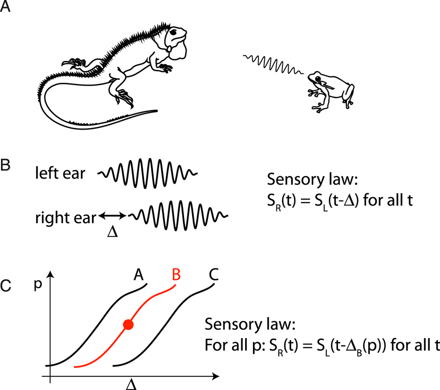
When a source produces a sound, two sound waves S L and S R arrive at the two ears, and these two sound waves have a particular property: they are delayed versions of each other (S L(t) = S R(t – Δ)) (Fig. 4B). In Gibsonian terminology, there is “invariant structure” in the sensory flow, which is to say that the signals obey a particular law. Thus, the sensory world of the iguana is made of random pairs of signals that follow particular laws that the iguana can identify. This identification is what Gibson called the “pick-up of information.” Evidently, “information” is not meant in the sense of Shannon but in the sense of laws or models of the sensory input. Note that the model in question is not a generative model as in predictive coding, but relations between observables, as in the models of physics.
A first interesting aspect of this alternative notion of information is that the topology of the world projects to the topology of sensory laws. By this, I mean that two different sounds produced by the frog at the same position will produce pairs of signals (S L, S R) that share the same property (the sensory law). This can be assessed without knowing what this property corresponds to in the world (i.e., the frog's position).
Thus, the iguana can observe sensory laws that have some particular properties, but do these laws convey any information about where the frog is? For an external observer, they certainly do, because the delay Δ is lawfully related to the frog's position. For the iguana, however, they do not because that lawful relation cannot be inferred from simply observing the acoustical signals. Therefore, this organism cannot have any sense of space, even though neural coding theories would pretend that it does, based on the correspondence between frog position and activity of the iguana's auditory neurons.
Let us now consider in addition that the iguana can turn its head (Fig. 4C). It can then observe a lawful relation between a proprioceptive signal (related to the head's position) and the observed delay Δ, which holds for some time (until the frog jumps to another position). Now when the iguana observes sounds with a particular delay, it can infer that if it were to move its head, then the delay would change in a particular predictable way. For the iguana, the relation between acoustical delay and proprioception defines the spatial position of the frog. We note that the perceptual inference involved here does not refer to a property in the external world (frog position), but to manipulations of an internal sensorimotor model.
Thus, the kind of information available to an organism is not Shannon information (correspondence to external properties of the world), but internal sensorimotor models. The interest of such models for the animal is that they can be manipulated to predict the effect of hypothetical actions.
3.4. Predictive coding and generative models
Predictive coding theory and its derivatives (Clark Reference Clark2013; Friston Reference Friston2010; Rao and Ballard Reference Rao and Ballard1999) propose that the brain encodes an internal model, which predicts the sensory inputs.Footnote 5 This seems to resemble the proposition put forward in the previous section. More precisely, neurons are thought to encode the variables of a hierarchical model of the inputs, in which higher-order neurons encode their prediction of the activity of neurons lower in the hierarchy, down to the sensory inputs. This prediction is subtracted from the input of lower-order neurons, so only the prediction error remains. This leads to a compressed representation of the inputs, and in this sense, it is a type of efficient coding theory.
This particular kind of model is called a generative model because its maps internal variables to the observables (sensory inputs), in contrast to the models of physics, which take the form of relations between observables (e.g., the ideal gas law, PV = nRT). Generative models are not the kind of internal models described in the previous section.
Consider the iguana with a fixed head. A generative model of the sensory inputs would map two internal variables S (sound) and Δ (interaural delay) to the two acoustical inputs S L and S R, as S L(t) = S(t), S R(t) = S(t – Δ). Neural activity encodes not the model itself but the coding variables Δ and S. In particular, neurons encode the entire sound S, even though it carries no information for the iguana (S is, by construction, random). This appears to contradict the claims of predicting coding theory: “To successfully represent the world in perception … depends crucially upon cancelling out sensory prediction error” (Clark Reference Clark2013, p. 7). Indeed, the success of a predictive code is evaluated by its ability to represent the input in a pictorial sense (as if it were a painting), but in this example, the numerical value of the signals provides no useful information beyond the relations they obey.
Consider now the case where the iguana can move its head. The internal model discussed in the previous section is S R(t) = S L(t – Δ x(p)) for all t, where x is the frog's position (Fig. 4C). The usefulness of this model stems from the fact that it can be manipulated; that is, on hearing a sound, the iguana can infer that, if it were to move its head to a new position p, the relation obeyed by the auditory signals would change in a predictable way. For example, the iguana can move its head so that S R = S L (“the frog is in front”). Thus, the kind of prediction that this model can produce is about relations between signals and not about the numerical value of the signals.
On the other hand, a generative model would map the coding variables S, x, and p to the sensory inputs S L(t) = S(t) and S R(t) = S(t – Δx(p)). This mapping is referred to as prediction and is instantiated by the feedback from higher-order neurons to lower-order neurons. This is not the same as predicting what action would make the two signals S L and S R match, which brings us to a discussion of the term predictive in predictive coding. The appeal of predictive processing is that making predictions seems to be a prerequisite to goal-directed behavior and, thus, a fundamental aspect of behavior. In fact, several authors have argued that anticipation is not simply a property of nervous systems, but even a fundamental property of life (Maturana and Varela Reference Maturana and Varela1973; Rosen Reference Rosen1985). For example, the iguana can predict how some properties of its sensory inputs should change if it were to turn its head. Consider this other example in human behavior: When someone is facing a cliff, she tends to slightly lean backward, because this posture makes it easier to move backward if necessary (Le Mouel and Brette Reference Le Mouel and Brette2017). But this is not at all the technical sense of “prediction” in predictive coding, as argued by Anderson and Chemero (Reference Anderson and Chemero2013). A neuron “predicts” the sensory inputs in the sense that its firing correlates with them; more specifically, a spike produced by a neuron leads to a subtraction of the expected input of a target neuron, which is the input occurring now, or possibly if we incorporate conduction delays, what will be happening after a fixed delay. This is not the kind of prediction implied by an anticipatory postural adjustment: If I change my posture in this way, then it will be easier to move backward in the hypothetical event that my balance is challenged.
In fact, what is useful for the organism is not literally to predict what will happen next, but rather what might happen next, conditionally on the actions I can do, so that I can select the appropriate action. But this requires manipulation of the model. For example, selection of an action requires instantiating the internal model with several possible values of action and then calculating the expected sensory variables. But this contradicts the proposition that neurons encode the “causes” of current sensory signals; to manipulate the model, encoding neurons would then have to be somehow disconnected from the sensory stream.
Technical work on predictive coding has focused exclusively on the technical senses of prediction and coding (correspondence); therefore, there is no empirical evidence that such codes might allow the organism to form predictions in a broader sense, nor is there any indication of how a theory based on neural coding might in principle explain anticipatory behavior.
3.5. Can neural codes represent structure?
The kind of representation of the world useful for adapted behavior is a structured internal model. Can neural codes possibly represent that structure? Memories and percepts are thought to be encoded by cell assemblies. In its basic and most popular form, a cell assembly is simply a specific subset of all neurons. When neurons of a cell assembly activate, the corresponding percept is formed (possibly indirectly by the activation of target neurons). This is the basic assumption of associative neural models of memory (Tonegawa et al. Reference Tonegawa, Liu, Ramirez and Redondo2015): Retrieving a memory consists of triggering activity in part of the memory-specific cell assembly (or “engram cells”), which then leads to the activation of all neurons in the assembly.
One problem with cell assemblies, in this simple form, is that they are unstructured and, thus, cannot represent structured internal models. The cell assembly model is analogous to the “bag of words” model in text retrieval, where a text is represented by its set of words and all syntax is discarded. In essence, a cell assembly is a “bag of neurons.” This causes a problem in representing not only the lawful structure of the world, but also the structure of any given perceptual scene. Consider, for example, the simple visual scene depicted in Figure 5. There is Paul, a person I know, wearing a new shirt, driving a car (Fig. 5). What is important here is that a scene is not simply a “bag of objects”; objects have relationships with each other, and there are many possible different relationships. For example, there is a car and there is Paul, and Paul is in specific relationships with the car, both a physical relationship (a particular posture within the car) and a functional relationship (driving it). Some of my behavior depends on identifying these relations because, for example, I can talk about them, and so if behavior relies on neural codes, then those codes should represent relations, not just the pixels of the image.
Perceptual scenes are highly structured. For example, there is Paul (person I know), driving a car and wearing a new shirt. Representing this scene by the firing of neural assemblies raises two issues: (1) It may be difficult to split active neurons into the correct assemblies (superposition catastrophe) and, more importantly, (2) the structure of the scene (relations shown by arrows) cannot be represented in this way.

But cell assemblies cannot represent these relations. Suppose there is a cell assembly that encodes “Paul” and another one that encodes “car.” To encode the driving relation between Paul and the car, a cell assembly that encodes “driving” would also be needed, but that assembly should also somehow refer to the two assemblies representing Paul and the car, and this is something that cannot be done with an unstructured bag of neurons (mathematically, one would need a labeled graph and not simply a subset of nodes).
This is related to the “binding problem,” although it is broader. If it is true that any given object is represented by the firing of a given assembly of neurons, then several objects should be represented by the firing of a larger assembly of neurons, the union of all assemblies, one for each object. Several authors have noted that this may lead to the “superposition catastrophe” (von der Malsburg Reference von der Malsburg1999); that is, there may be different sets of objects whose representations are fused into the same big assembly. One proposition is that the binding problem could be solved using retinotopic position as an object label; that is, neurons do not encode features but encode the conjunction of feature and retinotopic position (Kawato Reference Kawato, Ito, Miyashita and Rolls1997). However, this objection does not address the broader point, which is that cell assemblies encode objects or features to be related, but not the relations between them. In fact, it is known that current connectionist models, which are designed to optimally implement the idea that features are represented by the activity of one or several cells, cannot be trained to detect very simple relations between shapes in an image (Ricci et al. Reference Ricci, Kim and Serre2018).
The binding problem has led several authors to postulate that synchrony is used to bind the features of an object represented by neural firingFootnote 6 (Singer Reference Singer1999; von der Malsburg Reference von der Malsburg1999). This avoids the superposition catastrophe because at a given time, only one object is represented by neural firing. Synchrony is indeed a relation between neurons (mathematically, an equivalence relation). There are a few other examples in the neuroscience literature where synchrony is used to represent relations, although they are not usually cast in this way. One is the Jeffress (Reference Jeffress1948) model of ITD coding (Fig. 6A). In that model, neurons receive inputs from monaural neurons on the two sides, with different conduction delays. When input spikes arrive simultaneously, the neuron spikes. Thus, the neuron spikes when the two acoustical signals at the two ears are such that S L(t) = S R(t – d), where d is the conduction delay mismatch between the two ears. Physically, this corresponds to a sound source placed at a position such that it produces an ITD equal to d. In this model, the neuron's firing indicates whether signals satisfy a particular sensory law.
Neural representation of structure (adapted from Brette Reference Brette2012). (A) Jeffress’ model of sound localization. The sound arrives at the two ears with delays d L and d R. It is then transduced into spike trains that arrive at a binaural neuron with delays d L and d R. Synchrony occurs when d R – d L = δL – δR, making the neuron fire. (B) Synchrony receptive field. The response of a neuron to a stimulus is described as filtering of the sensory signal S through the receptive field N, followed by spiking. The synchrony receptive field of two neurons A and B with different receptive fields N A and N B is defined as the set of stimuli that elicit synchronous responses in these neurons.
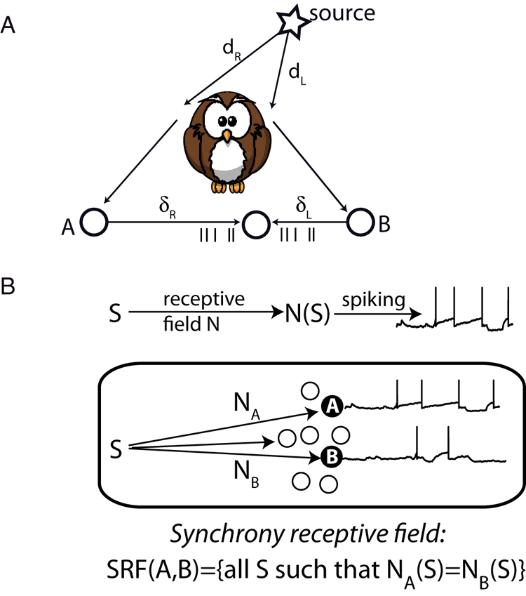
This interpretation of the model has been generalized with the concept of “synchrony receptive field” (Brette Reference Brette2012), which is the set of stimuli that elicit synchronous responses in a given group of neurons (Fig. 6B). One considers two neurons A and B that convert their time-varying inputs into precisely timed spike trains, where their inputs are seen as transformed versions N A(S) and N B(S) of the stimulus S (N A and N B are fixed and correspond to the receptive fields of the neurons). Synchrony between A and B then reflects (“encodes”) the sensory law N A(S) = N B(S). This framework has been applied to pitch perception (Laudanski et al. Reference Laudanski, Zheng and Brette2014) and to sound localization in realistic environments (Benichoux et al. Reference Benichoux, Fontaine, Karino, Joris and Brette2015; Goodman and Brette Reference Goodman and Brette2010).
Although synchrony can represent relations, neither binding by synchrony nor synchrony receptive fields solve the general problem (even theoretically), because only one type of relation can be represented by synchrony, and a symmetrical one: Does Paul drive the car, or does the car run over Paul? The fact that sentences can represent relations motivates the idea that the temporal structure of neural activity (e.g., the sequence of activated neurons, much like a sequence of words) could perhaps provide the adequate basis for structured neural representations (Buzsáki Reference Buzsáki2010). But this possibility remains speculative, and in particular, it remains to be demonstrated whether such hypothetical structures have the quality of representations that the brain can manipulate.
4. The causal structure of the coding metaphor
In the previous sections, I have argued that neural coding theories generally rely on the representational sense of the metaphor, the idea that neural codes are symbols standing for properties that the brain manipulates, but no evidence has been provided that this sense is valid. Worse, there is empirical evidence and theoretical arguments to the contrary.
Here I focus on a deeper problem with the neural coding metaphor. A striking characteristic of this metaphor is that it is a way to think about the brain independently of its causal structure. When we say, for example, that neurons encode the location of sounds, we talk about the activity of neurons without making any reference to the result of that activity or to the system of which the neurons are a component. I now examine the implications of this fact.
4.1. The dualistic structure of the coding metaphor
The coding metaphor has a dualistic structure. It structures the function of the brain into two distinct and dual components: the component that encodes the world into the activity of neurons, and the dual component that decodes that activity into the world or into actions in the world, as illustrated by the following examples: “Information that has been coded must at some point be decoded also; one suspects, then, that somewhere within the nervous system there is another interface, or boundary, but not necessarily a geometrical surface, where ‘code’ becomes ‘image’” (Somjen Reference Somjen1972, p. 3). “[I]nterpretation of the encoded information, typically consisting of its recoding by a higher-order set of neurons or of its “decoding” by an effector” (Perkel and Bullock Reference Perkel and Bullock1968, p. 307). “A stimulus activates a population of neurons in various areas of the brain. To guide behavior, the brain must correctly decode this population response and extract the sensory information as reliably as possible” (Jazayeri and Movshon Reference Jazayeri and Movshon2006, p. 690). “[T]he brain typically makes decisions … by evaluating the activity of large neuronal populations” (Quian Quiroga and Panzeri Reference Quian Quiroga and Panzeri2009, p. 173). “Ideal observers” used in many studies implement this dual-decoding brain.
Using the coding metaphor does not necessarily mean believing in dualism of body and mind,Footnote 7 but its dualistic structure has important consequences when it comes to understanding function. The two dual components (encoding/decoding) are indistinguishable in behavior, because no behavior involves just one of them. How then is it possible to attribute function to neural codes? How is it possible to draw conclusions about the neural basis of behavior from properties of neural codes, independently of the system in which the neurons are embedded? This is only possible by making an additional assumption, namely, that the encoding component has a function by itself (representing the inputs), somehow assigning the status of organ to a part of the nervous system. But there is no indication that the brain can be functionally decoupled in this way; neuroanatomy rather seems to invalidate this hypothesis.
To illustrate this point, I now discuss a concrete biological example. Paramecium is a unicellular organism that swims in stagnant fresh water using cilia and feeds on bacteria. It uses different kinds of sensory signals, including mechanical signals to avoid obstacles and chemical signals to localize food (Jennings Reference Jennings1906). To a first approximation, it alternates between straight courses and sudden random changes in direction (Fig. 7). It turns out that each change in direction is triggered by a spike produced by voltage-gated calcium channels (Eckert Reference Eckert1972). To find a chemical source, Paramecium uses a simple method: when concentration decreases, the membrane is depolarized by chemical receptors and a spike is produced (with some stochasticity), triggering a change of direction (similar to chemotaxis in Escherichia coli). This is of course a simplified description of Paramecium physiology and behavior, but for the sake of argument, we will consider an organism that functions in this simple way.
Spatial cognition in Paramecium, a “swimming neuron.” Paramecium finds a chemical source by switching to a new random direction when concentration decreases.

Paramecium is thus a sort of swimming neuron. Spiking activity varies lawfully with sensory signals (concentration) and, hence, encodes them in the same sense as a visual cortical neuron encodes visual signals. As for sensory neurons of the brain, we may argue that if the organism can navigate efficiently in its environment, then the spikes must contain information about that environment. Thus, it seems that the coding metaphor applies equally well to this swimming neuron as to any typical case in neuroscience.
Let us now think about functional questions. As an organism, Paramecium may have goals, for example, finding food. We may hypothesize that it achieves this goal efficiently, for example, by finding food as quickly as possible. To this end, sensory signals must be transformed into spikes in a specific way, which depends both on the goal (to move toward or away from a source, to look for food or to sleep, or to look for a mate) and on the effect of spikes on the organism's actions. Thus, there is a way to organize this system so that it achieves its function appropriately, which determines the transformation of inputs into spikes, that is, the neural code.
But if we now think of the neural code independently of the organism and environment that host it, we draw different conclusions. If the function of this neuron is to encode its input, then we may hypothesize that it achieves this function efficiently. This prescription determines a neural code that is specified by the statistics of inputs. Here the code depends neither on the goals of the animals nor on the effect of spikes on the organism's actions. It follows that this efficient code does not match, in general, the neural code that is adapted for the organism's goal. This mismatch occurs because function can be meaningfully ascribed to the organism as a system, but not necessarily to the components of this system.
This sensorimotor system is arguably much simpler than the brain; nevertheless, it demonstrates that the function of neurons cannot be meaningfully framed in terms of coding just because they respond to sensory stimuli. There is no indication that the brain is special in that it can be meaningfully separated into two dual components with independent functionality.
4.2. Coding versus causing
The Paramecium example highlights the fact that the neural coding metaphor is a way to think about the brain that is disconnected from its causal structure. Yet by postulating that neural codes are representations, we imply that these codes have a causal impact on the brain. This is also the case when neural codes are considered simply as transformations of inputs rather than explicit representations, as in Perkel and Bullock (Reference Perkel and Bullock1968, p. 227): “The problem of neural coding is defined as that of elucidating the transformations of information in the nervous system, from receptors through internuncials to motor neurons to effectors.” But does coding imply causing?
Consider, for example, the BOLD (blood oxygen level-dependent) signal, a property of blood used for functional brain imaging because it covaries with neural activity. The signal encodes visual signals in the same technical sense that the firing of neurons encodes visual signals. For example, one can “decode” the image from this signal (Naselaris et al. Reference Naselaris, Prenger, Kay, Oliver and Gallant2009). Yet, visual perception is not caused by the BOLD signal, which is why we do not consider that it is an internal representation used by the brain. Thus, not all coding variables have causal powers.
Consider the firing rate-versus-spike timing debate (Brette Reference Brette2015; Kumar et al. Reference Kumar, Rotter and Aertsen2010). This debate is generally formulated as follows: “Does the brain use a firing rate code or a spike timing code?” As the previous example illustrates, this is a largely irrelevant question because it focuses on correlations between stimuli and observables. We may as well ask Does the brain use the BOLD code? The relevant question is rather whether those observables have a causal role in the activity of the brain, and this involves a different set of arguments and answers (see Brette [Reference Brette2015] for a discussion). To see why, consider a sensorimotor system whose function is well understood in relation to its electrical activity: the heart (Fig. 8). The heart operates like a pump to circulate blood in two phases: the two atria contract, pushing blood into the ventricles (diastole); then the two ventricles contract, pushing blood into the pulmonary arteries (systole). These contractions are triggered by excitable cells in the atria and ventricles. For the heart to operate as a pump, cells in the two atria must spike synchronously, but out of phase with cells in the two ventricles. But the heart also responds to sensory stimulation. For example, the heart beats at a faster pace when we run. This means that the excitable cells of the heart encode running speed in their firing rate, in the technical sense. If we now look at the coding properties of these cells, we find that (1) firing rate is sensitive to running speed, (2) cells fire regularly, (3) spike timing is not reproducible between trials, and (4) spike timing (absolute or relative) carries no information about the stimulus beyond the rate. Thus, we would conclude that the heart uses a rate code. Yet, the temporal coordination of spikes is critical in this system; in fact, it is life critical. This paradox arises because the neural coding metaphor totally neglects the causal effect of spikes.
Operation of the heart. Atria simultaneously contract, triggered by synchronous firing of excitable cells; then ventricles simultaneously contract, pushing blood into the lungs.

If we want to describe the operation of the brain in terms of neural coding, the relevant question is whether the causal structure of neural codes is congruent with the causal structure of the brain.
4.3. Causal powers of coding variables
The causal structure of the brain is sketched in Figure 9A. At a coarse description level, the brain is a dynamical system coupled to the environment by circular causality. At a finer description level, the brain is itself made of neurons, which are themselves dynamical systems coupled together. To a first approximation, the coupling is mediated by spikes, which are timed events.
Causal structure of brain and neural codes. (A) The brain is a distributed dynamical system made of interacting neurons and is coupled to the environment by circular causality. A coding variable is a property of neural activity, which is implicitly assumed to have a causal effect on the brain. (B) Neural codes are linked together and with the world by linear causality.
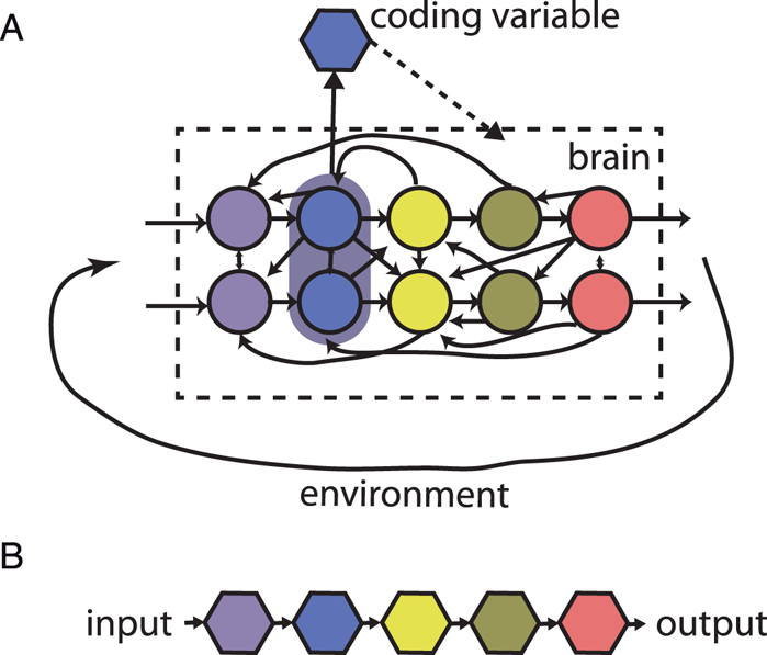
Consider the proposition “the firing rate of neuron A encodes the location of a sound source,” corresponding to some empirically observed correlation. The implication that this information is decoded by the brain relies on the presupposition that the coding variable “firing rate of neuron A” causally influences the future activity of the brain. Spikes, of course, have causal effects on the brain. But a neural coding variable (“firing rate of neuron A” or “relative activity of two neural populations”) is a particular measurement of spiking activity, and the question is whether that particular measurement has causal powers.
Empirically, a coding variable is an aggregate variable based on measurements of spiking activity over some time, space, and possibly trials. An example of integrating over trials (and time) is a neuron that responds specifically to pictures of Jennifer Anniston in various poses (Quian Quiroga et al. Reference Quian Quiroga, Reddy, Kreiman, Koch and Fried2005). But only on average: the coding variable is the median number of spikes across trials between 300 and 1,000 ms after stimulus onset. On a given trial, the neuron might not be firing at all. Unless the subject was not perceiving the actress in those trials, this implies that this neuron cannot encode the percept “Jennifer Anniston” in the sense of causing the percept. Rather, its firing correlates (on average) with the presentation of pictures of Jennifer Anniston, which is already a notable fact. Perceptual representations cannot be based on averages; percepts are experienced now, not on average. Neural codes based on averaging over trials do not have causal powers (see also Gomez-Marin and Mainen Reference Gomez-Marin and Mainen2016). In the same way, a firing probability (one abstract way to define a neuron's firing rate) does not have causal powersFootnote 8; only the occurrence of firing does.
An example of integrating over space (and time) is when we propose that the position of a sound source is encoded by the difference in total activity between the two symmetrical inferior colliculi (Grothe et al. Reference Grothe, Pecka and McAlpine2010). This coding variable indeed varies when source position is changed (Thompson et al. Reference Thompson, von Kriegstein, Deane-Pratt, Marquardt, Deichmann, Griffiths and McAlpine2006). Does it mean that it has causal powers, that is, that it determines sound localization behavior? It seems implausible, first, as previously discussed because it also varies with other properties of sounds, and second, because electrical stimulation in the inferior colliculus triggers orienting responses that vary with the place of stimulation, whereas stronger stimulation results in orienting responses that engage a larger part of the body (one pinna, both pinnae, and eyes, in order of recruitment) (Syka and Straschill Reference Syka and Straschill1970). Thus, there is no guarantee that a coding variable obtained by integrating over neurons has causal powers.
But the key difficulty is time. The course of a dynamical system is determined by its current state, which is characterized by state variables such as membrane potential and the state of ionic channels. Spikes, on the other hand, are events (something happening to the system) and not properties (some characteristic of the system). Therefore, spiking activity is not something defined at any point in time, which could give it the causal role of a state variable, but something that is measured over some predefined period (in the first example, 300 to 1,000 ms after stimulus onset). Empirically, a neural coding variable is necessarily anchored to the temporality of the experiment (some window of time after the onset of the stimulus). Once we have anchored variables in time, all possibility of physical interaction between coding variables disappears: if variables X and Y are defined over two different time windows T 1 and T 2, then there cannot be causal influence in both directions (X→Y and Y→X). But neurons mutually influence themselves over timescales of a few milliseconds, without waiting for the coding variable to be defined or for a stimulus to be presented. Neural codes abstract time away, but temporality is critical to the operation of a dynamical system.
4.4. Causal structure of neural codes
If neural coding variables are anchored in time, then the only possible causal structure linking coding variables is a linear sequence of transformations (Fig. 9B). This is implicit in Perkel and Bullock's (Reference Perkel and Bullock1968) definition of neural coding (“transformations … from receptors through internuncials to motor neurons to effectors”). This linear structure is also implicit in any claim that a stimulus is encoded, then decoded: cognition follows a linear causal flow,Footnote 9 from stimulus to perception to action (Hurley Reference Hurley2001). In such descriptions, the temporality of the physical system has disappeared and has been replaced by the discrete temporality of an algorithm, which is disconnected from physical time. In other words, this is an algorithmic description. But as van Gelder (Reference van Gelder1995) pointed out, dynamical systems cannot in general be mapped to algorithmic descriptions.Footnote 10
The coding metaphor tries to match the causal structure of dominoes to the causal structure of a tent, where the states of different elements are co-determined (Fig. 10). In addition to the coupling of neurons, the brain itself is coupled to its environment; that is, there is circular and not linear causality (Fig. 9A). As Dewey (Reference Dewey1896, p. 363) pointed out more than a century ago, “the motor response determines the stimulus, just as truly as sensory stimulus determines the movement.” Many other authors in biology, psychology, philosophy, and robotics have argued that perception is not a one-way process but an interaction with the environment (Ahissar and Assa Reference Ahissar and Assa2016; Brooks Reference Brooks1991a; Gibson Reference Gibson1979; O'Regan and Noë Reference O'Regan and Noë2001; Powers Reference Powers1973a). This makes the proposition that neural activity encodes stimuli questionable. In fact, it makes the very notion of stimulus questionable, as it seems to give no role for spontaneous activity other than noise (Deco et al. Reference Deco, Jirsa and McIntosh2011), when autonomous activity is central to the organization of behavior. As a theory of cognition, the neural coding metaphor seems to embrace the most basic form of behaviorism.Footnote 11
The causal structure of the neural coding metaphor is that of dominoes (A), but the causal structure of the brain rather resembles that of a tent (B).

5. Conclusion
5.1. Summary
When I say that the heart is a pump, I propose a function for the heart (to circulate blood) and mechanisms by which blood is circulated; I propose specific ways in which elements of the heart interact by identification with elements of a pump. In effect, the pump is a model of the heart. A metaphor is not simply words arbitrarily chosen to designate an object; it is a model of the object (Lakoff and Johnson Reference Lakoff and Johnson1980a), and as such it deserves scrutiny as does any other model in science. Is coding a good model of brain function?
There are three aspects of the coding metaphor: correspondence, representation, and causality. Technical results are based on the first aspect, but their interpretation and claimed significance draw on the two other aspects, which are not subject to the same scrutiny. Many neural coding theories rely on the idea that the brain manipulates neural representations of stimulus properties, as if the variable of a neural code were a processor register that the brain can store, retrieve, and combine arbitrarily, while knowing what the variable refers to. But what is the evidence that such neural representations exist, and what is the evidence that the brain can manipulate spikes in this way?
Technically, it is found that the activity of many neurons varies with stimulus parameter, but also with sensory, behavioral, and cognitive context; neurons are also active in the absence of any particular stimulus. A tight correspondence between stimulus property and neural activity only exists within a highly constrained experimental situation. Thus, neural codes have much less representational power than generally claimed or implied. Behavioral significance is obtained only by making an implicit “linking proposition” (Teller Reference Teller1984) that relates coding variables and behavior, which takes the form of a “decoder.” The decoder, often an “ideal observer,” is a hypothetical abstract construct whose biological basis is unspecified and whose existence is unquestioned, even though the decoder must incorporate key contextual aspects, including methodological details of the experiment, which defines the coding variables. Critically, the contextual dependence of neural codes cannot be solved by incorporating contextual variables in a broader neural code, because context is precisely what defines the variables. A perceptual scene cannot be fully defined as a vector of properties. Properties of what?
The notion of information implied by the coding metaphor is inappropriate in understanding perception and behavior, because it is information by reference to external symbols (Bickhard Reference Bickhard2009). A more appropriate notion is information as organization (Thompson Reference Thompson1968), namely, relations between sensory signals and actions, forming a structured internal model. The relation between such structured models of the world and neural activity is unclear, but what is clear is that no neural coding theory proposed so far seems adequate, even in principle.
Ultimately, the neural coding metaphor is a way to think about the brain that is disconnected from its causal structure. The brain is a dynamical system coupled to the environment and is itself composed of coupled dynamical systems (neurons), whose interaction is mediated by spikes, which are timed events. The dualistic structure of the metaphor cuts through this organization and decides that one part of the brain can be understood independently of the way it interacts with the rest of the brain and independently of the way the brain interacts with the world. More fundamentally, a causal role is attributed to coding variables, but this is incoherent because coding variables are extended measurements of activity linked to the temporality of experiments; they are not causal variables of the underlying dynamical system. In conclusion, the causal structure of neural coding metaphor is incongruent with the causal structure of the brain. If neural codes have no causal power, then they cannot form a valid basis of a theory of brain function.
5.2. What else, if not coding?
Since the coding metaphor is so ingrained in neuroscience, how could it be possible to abandon it? What could it be replaced with?
First, that there is no simple substitute for neural coding does not make it a viable option. The neural coding metaphor is attractive partly because it resonates with Cartesian philosophy, as pointed out by Cisek (Reference Cisek1999), and partly because it seems to fit with the computational view of the mind, the idea that cognition is the manipulation of symbols that represent properties of objects in the world. But the symbols provided by neural codes are not context free; they are unstructured and they have no causal powers. They do not have the quality required by the computational view. Thus, the appeal of the neural coding metaphor is illusory. Even if it were possible to map brain activity to computational descriptions, neural codes would not provide the adequate mapping.
Similar arguments have been made against the idea of a genetic code (or genetic program), and the alternative route is to adopt a systemic approach (Noble Reference Noble2008). The brain is a system, or, more accurately, the brain, body and environment are a system. This approach is precisely what the coding metaphor forbids, because it cuts through the system and uncouples its different components. Since it is a dynamical system, this view is related to the dynamical view of cognition (van Gelder Reference van Gelder1998). But the specific point here is not so much that cognition is dynamic, but rather that its neural basis is a dynamical system and must be understood as such. It is a special kind of dynamical system in that it is composed of units (neurons), which are also dynamical systems. The causal role of spikes in this system is to mediate coupling between these dynamic units. They are transient events that are better understood as actions than as representations. A useful analogy then might be collective behavior: social insects are also dynamical systems coupled to each other by actions, and the collective behavior they display can be understood in terms of self-organization without resorting to the concept of coding (Bonabeau et al. Reference Bonabeau, Theraulaz, Deneubourg, Aron and Camazine1997). This view should not be mistaken for an argument against representations in general, but more precisely against the classic view of representations as encodings. Bickhard (Reference Bickhard2015c), in particular, has made a case for representations as a form of normativity realized by anticipatory properties of internal processes.
In terms of neural modeling, this requires considering sensorimotor systems. The necessity of this level of analysis has been stressed by a number of authors who have developed alternative views on cognition (Ahissar and Assa Reference Ahissar and Assa2016; Bickhard and Terveen Reference Bickhard and Terveen1996; Brooks Reference Brooks1991a; Gibson Reference Gibson1979; Hurley Reference Hurley2001; Maturana and Varela Reference Maturana and Varela1973; O'Regan and Noë Reference O'Regan and Noë2001; Pezzulo and Cisek Reference Pezzulo and Cisek2016; Powers Reference Powers1973a). Paradoxically, it is customary in systems neuroscience to model perceptual abilities by considering only the corresponding sensory areas. We speak, for example, of the visual system as a set of anatomical structures from the eye to the visual cortex. But the visual system defined in this way is not actually a system if it is disconnected from the elements without which it cannot have any function. It follows that models of perceptual systems are in effect not biological models, but chimeras obtained by attaching a neural model of a sensory area to an abstract construct (“decoder”) that maps the activity of neurons to descriptors of behavior and, often, to an even more problematic abstract construct (“encoder”) that maps stimulus parameters to model inputs. This methodology embraces both behaviorism (neural activity is only responses to stimuli) and dualism (something else makes sense of neural activity). Instead, I suggest developing models of the full sensorimotor loop, “models that behave” (Gomez-Marin Reference Gomez-Marin, Çelik and Wernet2017). For example, instead of looking for neural codes of sound location, one could look for neural models of auditory orientation reflexes. Measurements of neural activity in stimulus-response experiments can be used to constrain and test such models, but they do not need to be the output of the model, nor do they need to be a causal variable in the model. To be clear, the issue is not about the amount of detail that needs to be incorporated. Models can be simplified or idealized, as any model needs to be. The issue is to respect the causal structure of brain and behavior and to see neural activity as what it really is: activity. Action potentials are potentials that produce actions; they are not hieroglyphs to be deciphered.


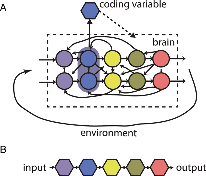




Target article
Is coding a relevant metaphor for the brain?
Related commentaries (27)
A clash of Umwelts: Anthropomorphism in behavioral neuroscience
A sensorimotor alternative to coding is possible
Abandoning the code metaphor is compatible with semiotic process
Beyond metaphors and semantics: A framework for causal inference in neuroscience
Beyond Neural Coding? Lessons from Perceptual Control Theory
Codes are for messages, not for neurons
Codes, communication and cognition
Codes, functions, and causes: A critique of Brette's conceptual analysis of coding
Encodingism is not just a bad metaphor
Extrinsic and intrinsic representations
From mental representations to neural codes: A multilevel approach
From the “coding metaphor” to a theory of representation
Generative models as parsimonious descriptions of sensorimotor loops
How can we play together? Temporal inconsistencies in neural coding of music
Is coding a relevant metaphor for building AI?
Is information theory, or the assumptions that surround it, holding back neuroscience?
Is “the brain” a helpful metaphor for neuroscience?
Modest and immodest neural codes: Can there be modest codes?
Neural code: Another breach in the wall?
Neural codes – Necessary but not sufficient for understanding brain function
Not just a bad metaphor, but a little piece of a big bad metaphor
Our understanding of neural codes rests on Shannon's foundations
Plasticity of the neural coding metaphor: An unnoticed rhetoric in scientific discourse
Prediction, embodiment, and representation
Quantifying the role of neurons for behavior is a mediation question
The Bayesian brain: What is it and do humans have it?
The origin of the coding metaphor in neuroscience
Author response
Neural coding: The bureaucratic model of the brain