1 Introduction
Nowadays, microfluidics is undergoing rapid expansion due to deeper control of operating conditions and the possibility of continuous production. Microfluidic devices are present in a wide range of applications, examples of which spanning from dissolution of carbon dioxide in microchannels (Cubaud & Ho Reference Cubaud and Ho2004; Chi et al. Reference Chi, Johnstone, Voicu, Mehlmann, Dielmann, Kumacheva and Stephan2017; Durgadevi & Pushpavanam Reference Durgadevi and Pushpavanam2018), to culture of cells (Mehta et al. Reference Mehta, Mehta, Sud, Song, Bersano-Begey, Futai, Heo, Mycek, Linderman and Takayama2007), adsorption kinetics of surfactants (Riechers et al. Reference Riechers, Maes, Akoury, Semin, Gruner and Baret2016), polymerisation of monodisperse beads by solvent diffusion from droplets (Hung et al. Reference Hung, Teh, Jester and Lee2010), and boiling and condensation in microchannels (Kandlikar et al. Reference Kandlikar, Garimella, Li, Colin and King2005). Despite the apparent unrelatedness of these examples, they have important similarities. In effect, objects such as bubbles, cells or drops are immersed in a liquid flowing in small microchannels and there exists an exchange of mass/heat between these objects and the surrounding liquid. Besides microfluidics, other phenomena also rely on mass/heat transfer in microchannels such as microrocket production (Gallino et al. Reference Gallino, Gallaire, Lauga and Michelin2018), oxygen transport by red blood cells in capillaries (Vadapalli, Goldman & Popel Reference Vadapalli, Goldman and Popel2002), and the control of the nucleation and full dissolution of bubbles in extracorporeal medical devices, whose presence in blood may lead to gas embolism (Barak & Katz Reference Barak and Katz2005). Thus, it is of high importance to control the transfer mechanisms governing all these processes.
Kuo & Chiu (Reference Kuo and Chiu2011) provide a review of available techniques for the control of mass transport in microfluidics. Most of them rely on very sophisticated geometries or on the tailoring of surface rheological properties (Beltramo et al. Reference Beltramo, Gupta, Alicke, Liascukiene, Gunes, Baroud and Vermant2017). In this work, we consider the mass transfer of bubbles in cylindrical microchannels (i.e. straight microchannels with a circular cross-section) and study the influence of all the properties of the system in a systematic manner using numerical means. To understand this problem, the hydrodynamics and the dissolution are studied in two different steps. The hydrodynamics has been previously reported in Rivero-Rodriguez & Scheid (Reference Rivero-Rodriguez and Scheid2018a ,Reference Rivero-Rodriguez and Scheid b ).
The dissolution of
 $\text{CO}_{2}$
in water flowing in microchannels has recently drawn the attention of many researchers (Cubaud, Sauzade & Sun Reference Cubaud, Sauzade and Sun2012; Shim et al.
Reference Shim, Wan, Hilgenfeldt, Panchal and Stone2014; Ganapathy et al.
Reference Ganapathy, Shooshtari, Dessiatoun, Alshehhi and Ohadi2014; Mikaelian, Haut & Scheid Reference Mikaelian, Haut and Scheid2015b
). Despite the fact that larger-scale systems, such as column reactors, have been studied for several decades (Griffith Reference Griffith1960; Deckwer Reference Deckwer1980), bubble dissolution is still a matter of active research because of its rich dynamics (Auguste & Magnaudet Reference Auguste and Magnaudet2018) implying various dissolution regimes (Dhotre & Joshi Reference Dhotre and Joshi2004). The miniaturisation of bubble columns is known to increase the mass transfer for both gas–liquid (Durgadevi & Pushpavanam Reference Durgadevi and Pushpavanam2018) and liquid–liquid (Xu et al.
Reference Xu, Tan, Li and Luo2008) exchanges, which increases the reaction rate in mass transfer limited reactors (Kashid, Renken & Kiwi-Minsker Reference Kashid, Renken and Kiwi-Minsker2011). In the case of bubbles in microchannels, few hydrodynamic regimes have been found (Cubaud & Ho Reference Cubaud and Ho2004; Abiev Reference Abiev2013) relative to the size and ordering of the bubbles, or relative to coalescence (Cubaud & Ho Reference Cubaud and Ho2004). Concerning the dissolution of a train of bubbles, the pure diffusion has been considered by Shim et al. (Reference Shim, Wan, Hilgenfeldt, Panchal and Stone2014) as well as its dissolution through a boundary layer by Mikaelian, Haut & Scheid (Reference Mikaelian, Haut and Scheid2015a
). However, a characterisation of all the different dissolution regimes is lacking in the literature.
To understand the dissolution of a train of bubbles flowing inside a microchannel, it is crucial to understand the mass transfer around each bubble. In this work we provide a complete picture of the mass transfer of the gas around bubbles in microchannels covering the entire range of experimentally relevant distance between bubbles as well as Péclet numbers from small to large values. This is useful for the control of this phenomenon in many applications such as reactions in bubbly flow (Hashemi, Modestino & Psaltis Reference Hashemi, Modestino and Psaltis2015) or controlling the oxygen level of cells (Mehta et al. Reference Mehta, Mehta, Sud, Song, Bersano-Begey, Futai, Heo, Mycek, Linderman and Takayama2007). Modelisation of similar situations has already been carried out for the design of biosensors (Squires, Messinger & Manalis Reference Squires, Messinger and Manalis2008), for the control of glucose concentration in a culture of cells (Westerwalbesloh et al. Reference Westerwalbesloh, Grünberger, Stute, Weber, Wiechert, Kohlheyer and von Lieres2015) or drug delivery (Gekle Reference Gekle2017).
Heat and mass transfers in fluid flows have been widely studied in many simple geometries (Rohsenow, Hartnett & Ganic Reference Rohsenow, Hartnett and Ganic1985) in which the relation between the transfer coefficient and the convection to diffusion ratio are provided by analytical/numerical or experimental means. However, full numerical simulations sometimes become an alternative for complex geometries despite the higher computation cost. This cost can be decreased with the help of a multi-scale approach. In this approach, small and large scales are considered separately. At small scale, the local details of the geometries are considered and the relation between the mass transfer coefficient and the convection to diffusion ratio is obtained. Then, using this relation, the concentration of dissolved species is obtained for the large scale, taking into account the entire geometry. At the large scale other domains and physical behaviours can also be considered.
This approach has already been used for the dissolution of bubbles in microchannels by Mikaelian et al. (Reference Mikaelian, Haut and Scheid2015a ,Reference Mikaelian, Haut and Scheid b ). The small scale is at the level of the bubble (Mikaelian et al. Reference Mikaelian, Haut and Scheid2015a ), and they provide the correlation for the Sherwood number as a function of the Péclet number for non-interacting bubbles and large values of the Péclet number. A model is built for the large scale (Mikaelian et al. Reference Mikaelian, Haut and Scheid2015b ), at the level of the position along the microchannel, in which, in addition to the previous correlation, also the ideal gas law, Henry’s law and the mass balance of the bubble are implemented. The concentration of gas in the carrier liquid and the size distribution of the bubble along the channel can then be computed.
The aim of this work is twofold: to cover the entire range of Péclet numbers and to investigate the influence of the distance between bubbles on the mass transfer rate at the scale of the bubble, i.e. on the Sherwood number. The dissolution at the scale of the microchannel is beyond the scope of this work, and we confine ourselves to some comments in a section at the end of the paper.
The structure of the paper is as follows. In § 2 we present the model we use to describe the dynamics and mass transfer at the scale of a bubble of finite size and explain the underlying hypotheses (§ 2.1), scaling (§ 2.2), models for the hydrodynamics (§ 2.3) and mass transfer (§ 2.4). In § 3 we present the results on the transient behaviour of the mass transfer and motivate the modal expansion. In § 4, using the modal expansion, we study the effect of all the parameters on the mass transfer of bubbles under the hypotheses of stress-free and spherical interface, Stokes flow and centred bubbles. We provide a qualitative description of the different mass transfer regimes and characterise it depending on the importance of diffusion along the streamlines. On the one hand, the behaviour for small
 $Pe$
numbers, implying that the diffusion along the streamlines is not negligible as compared to convection, is presented in § 4.1, including a simplified model. On the other hand, the behaviour for large
 $Pe$
is presented in § 4.2. In this case, convection dominates along the streamlines direction, and thus crosswind diffusion becomes crucial to govern the mass transfer through a boundary layer or the remaining wake behind the bubbles. We also studied the effects of a small distance between bubbles in § 4.3. In § 5 we show the contribution of the different modes to the mass transfer. In § 6 we consider some extensions of the previous model, such as the limit of a rigid interface in § 6.1, the deformability in § 6.2, the inertial forces in § 6.3 and off-centred positions in § 6.4. In § 7 these results are brought to bear on the dissolution process at the scale of a microchannel. Finally, Section 8 concludes.
2 Modelling
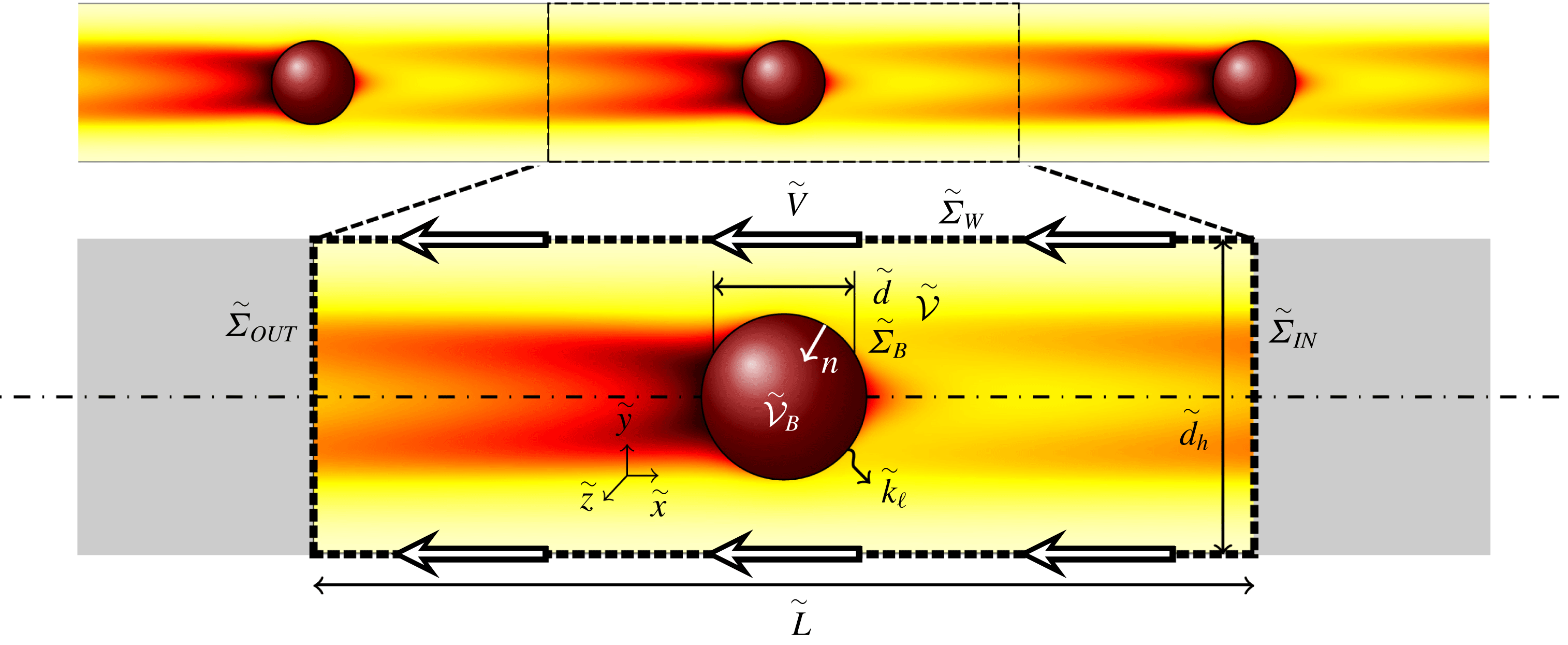
We study the mass transfer of a train of bubbles in a cylindrical microchannel at the scale of the bubble. To model this situation, we solve the steady Stokes equations and the unsteady advection–diffusion equation on a periodic volume
 $\tilde{{\mathcal{V}}}$
of length
 $\tilde{L}$
containing one single bubble of volume
 $\tilde{{\mathcal{V}}}_{B}$
, attached to it and delimited by the walls of the channel,
 $\tilde{\unicode[STIX]{x1D6F4}}_{W}$
, two cross-sections of the channel,
 $\tilde{\unicode[STIX]{x1D6F4}}_{IN}$
and
 $\tilde{\unicode[STIX]{x1D6F4}}_{OUT}$
, and the surface of the bubble,
 $\tilde{\unicode[STIX]{x1D6F4}}_{B}$
, as schematised in figure 1. Equivalent diameters are defined as referred to the volume,
 $\tilde{{\mathcal{V}}}_{B}=(\unicode[STIX]{x03C0}/6)\tilde{d}^{3}$
, or to the surface,
 $\tilde{\unicode[STIX]{x1D6F4}}_{B}=\unicode[STIX]{x03C0}\tilde{d}_{\unicode[STIX]{x1D6F4}}^{2}$
. We consider a liquid of constant properties, such as viscosity
 $\tilde{\unicode[STIX]{x1D707}}$
, surface tension
 $\tilde{\unicode[STIX]{x1D6FE}}$
, isotropic gas diffusivity in the liquid
 $\tilde{D}$
, saturation concentration of the gas in the liquid
 $\tilde{C}_{sat}$
and initial concentration
 $\tilde{C}_{0}$
. It flows inside a channel of diameter
 $\tilde{d}_{h}$
with a mean flow velocity
 $\tilde{J}$
. This flow produces a pressure drop along the period
 $\tilde{L}$
of the microchannel in the axial direction
 $\tilde{x}$
, due to the Poiseuille flow,
 $-\tilde{L}\unicode[STIX]{x2202}_{\tilde{x}}\tilde{p}_{P}$
, modified by the presence of one bubble,
 $\unicode[STIX]{x0394}\tilde{p}$
. The bubble travels at the velocity
 $\tilde{V}$
, resulting from the equilibrium of the bubble in the axial direction, and the mass transfer is characterised by the mass transfer coefficient
 $\tilde{k}_{\ell }$
. Consequently, the three values,
 $\tilde{V}$
,
 $\tilde{k}_{\ell }$
and
 $\unicode[STIX]{x0394}\tilde{p}$
, are numerically determined. First, we consider a stress-free and non-deformable spherical interface, in the case of a Stokes flow and centred bubbles. Later, in § 6, we extend the model to consider a rigid interface, deformable interface, inertial forces and off-centred bubbles.
Sketch of the modelled segment of a train of bubbles in a microchannel. A typical concentration field obtained from numerical simulations is represented in the colormap, where dark red corresponds to saturation concentration and light yellow to lower concentration.

2.1 Hypotheses
It is assumed that (i) the bubble size in a dissolving train of bubbles decreases much more slowly than the mass transfer time scale. It allows us to freeze the bubble diameter, and consequently also the flow field, to characterise the mass transfer. The hydrodynamics and the geometry are quasi-steady, and quasi-periodic as a consequence of the quasi-steadiness. In addition, we assume that (ii) the difference between the transferred mass of two consecutive bubbles, which is due to the difference in time they have been transferring mass, is small compared to the mass to be dissolved. This allows us to consider that the concentration of gas in the liquid around the bubble is also quasi-periodic. These hypotheses are referred hereafter as (i) quasi-steadiness and (ii) quasi-periodicity. They allow us to decouple the mass transfer (i.e. the mass transfer coefficient) and the dissolution process (i.e. the change of bubble size), as already done in work by Mikaelian et al. (Reference Mikaelian, Haut and Scheid2015a ,Reference Mikaelian, Haut and Scheid b ). In the present work, we focus on the mass transfer.
Additionally, since the mass transfer is decoupled from the dissolution of the bubble, different physical phenomena can be studied in addition to the bubble dissolution, such as the polymerisation of monodisperse beads by solvent diffusion from droplets (Hung et al. Reference Hung, Teh, Jester and Lee2010), nutrient intake by cells (Michelin & Lauga Reference Michelin and Lauga2011) independently of its metabolism, cell breath, drug delivery, bioreactions, etc.
2.2 Scaling
In this work, quantities with tildes are dimensional and quantities without tildes are their dimensionless counterparts considering the characteristic length, velocity and pressure as the hydraulic diameter of the channel
 $d_{h}$
, the mean flow velocity
 $\tilde{J}$
and the viscous stress
 $\tilde{\unicode[STIX]{x1D707}}\tilde{J}/\tilde{d}_{h}$
, respectively. Note that
 $\tilde{J}(\unicode[STIX]{x03C0}/4)\tilde{d}_{h}^{2}=\tilde{Q}_{L}+\tilde{Q}_{G}$
, where
 $\tilde{Q}_{L}$
and
 $\tilde{Q}_{G}$
are the liquid and gas flow rates, respectively. We then have the dimensionless numbers
 $$\begin{eqnarray}Pe=\frac{\tilde{J}\tilde{d}_{h}}{\tilde{D}},\quad d=\frac{\tilde{d}}{\tilde{d}_{h}},\quad L=\frac{\tilde{L}}{\tilde{d}_{h}},\end{eqnarray}$$
where
 $Pe$
is the Péclet number. The choice of the convective velocity as the characteristic one does not allow the numerical limit of
 $Pe\rightarrow 0$
. However, the results are independent of the
 $Pe$
numbers for sufficiently small
 $Pe$
which then represents the limit
 $Pe\rightarrow 0$
.
It is worth noting that
 $t$
is the time made dimensionless with the convective time scale whereas
 $tPe^{-1}$
is the time made dimensionless with the diffusive time scale. The dimensional mass transfer coefficient can be written as
 $\tilde{k}_{\ell }=Sh\,\tilde{D}/\tilde{d}$
, where
 $Sh$
is the Sherwood number, defined later by (2.12) in § 2.4.
2.3 Modelling of the hydrodynamics
According to the previous description, the liquid flow around the bubble in a channel segment of length
 $L$
,
 $L$
being the distance between two consecutive bubbles from centre to centre, can be analysed by solving the continuity and the steady Stokes equations,
 $$\begin{eqnarray}\displaystyle & \displaystyle \unicode[STIX]{x1D735}\boldsymbol{\cdot }\boldsymbol{v}=0\quad \text{at }{\mathcal{V}}, & \displaystyle\end{eqnarray}$$
 $$\begin{eqnarray}\displaystyle & \displaystyle \mathbf{0}=-\unicode[STIX]{x1D735}p+\unicode[STIX]{x1D735}\boldsymbol{\cdot }\unicode[STIX]{x1D749}\quad \text{at }{\mathcal{V}}, & \displaystyle\end{eqnarray}$$
 $p$
,
 $\boldsymbol{v}$
and
 $\unicode[STIX]{x1D749}=\unicode[STIX]{x1D735}\boldsymbol{v}+(\unicode[STIX]{x1D735}\boldsymbol{v})^{\text{T}}$
are the pressure, the velocity vector and the viscous stress tensor, respectively.
In the reference frame attached to the bubble moving at the velocity
 $V$
in the axial direction, the velocity of the liquid at the wall is written as
 $$\begin{eqnarray}\boldsymbol{v}(\boldsymbol{x})=-V\boldsymbol{e}_{x}\quad \text{at }\unicode[STIX]{x1D6F4}_{W}.\end{eqnarray}$$
The velocity
 $V$
is the one leading to the hydrodynamic equilibrium in the axial direction for the bubble,
 $$\begin{eqnarray}\int _{\unicode[STIX]{x1D6F4}_{B}}(-p\boldsymbol{n}+\boldsymbol{n}\boldsymbol{\cdot }\unicode[STIX]{x1D749})\boldsymbol{\cdot }\boldsymbol{e}_{x}\,\text{d}\unicode[STIX]{x1D6F4}=0,\end{eqnarray}$$
where
 $\boldsymbol{n}$
and
 $\text{d}\unicode[STIX]{x1D6F4}$
are the outer normal and the differential surface, respectively.
The velocity profile and pressure gradient are periodic in the axial direction with period
 $L$
. Consequently, the pressure field between two different cross-sections differs by a constant pressure, and the boundary conditions are
 $$\begin{eqnarray}\displaystyle & \displaystyle p(\boldsymbol{x}+L\boldsymbol{e}_{x})=p(\boldsymbol{x})-\unicode[STIX]{x0394}p+L\unicode[STIX]{x2202}_{x}p_{P}\quad \text{at }\unicode[STIX]{x1D6F4}_{cross}, & \displaystyle\end{eqnarray}$$
 $$\begin{eqnarray}\displaystyle & \displaystyle \boldsymbol{v}(\boldsymbol{x}+L\boldsymbol{e}_{x})=\boldsymbol{v}(\boldsymbol{x})\quad \text{at }\unicode[STIX]{x1D6F4}_{cross}, & \displaystyle\end{eqnarray}$$
 $$\begin{eqnarray}\displaystyle & \displaystyle \unicode[STIX]{x2202}_{x}\boldsymbol{v}(\boldsymbol{x}+L\boldsymbol{e}_{x})=\unicode[STIX]{x2202}_{x}\boldsymbol{v}(\boldsymbol{x})\quad \text{at }\unicode[STIX]{x1D6F4}_{cross}, & \displaystyle\end{eqnarray}$$
 $\unicode[STIX]{x1D6F4}_{cross}$
is any cross-section and the pressure drop along the period
 $L$
is due to the Poiseuille flow, i.e.
 $\unicode[STIX]{x2202}_{x}p_{P}=-32$
in cylindrical microchannels, modified by the presence of the bubble,
 $\unicode[STIX]{x0394}p$
. The mean flow velocity is defined by
 $$\begin{eqnarray}\int _{\unicode[STIX]{x1D6F4}_{cross}}(\boldsymbol{v}\boldsymbol{\cdot }\boldsymbol{e}_{x}+V-1)\,\text{d}\unicode[STIX]{x1D6F4}=0,\end{eqnarray}$$
where it is worth noting that since the mean flow velocity has been chosen as the characteristic velocity, it corresponds to the unity term. Note that
 $\unicode[STIX]{x0394}p$
is unknown and that (2.5)–(2.6) must be imposed only at one arbitrary cross-section because of the periodicity. The solution is independent of the convenient choice of the position of
 $\unicode[STIX]{x1D6F4}_{cross}\equiv \unicode[STIX]{x1D6F4}_{OUT}$
and the centre of the bubble at
 $x=0$
.
The stress-free boundary conditions involve no stresses in the tangential direction and the impermeability condition in the normal direction, which are written as
 $$\begin{eqnarray}\displaystyle & \displaystyle -p\boldsymbol{n}+\boldsymbol{n}\boldsymbol{\cdot }\unicode[STIX]{x1D749}=-p_{S}\boldsymbol{n}\quad \text{at }\unicode[STIX]{x1D6F4}_{B}, & \displaystyle\end{eqnarray}$$
 $$\begin{eqnarray}\displaystyle & \displaystyle \boldsymbol{n}\boldsymbol{\cdot }\boldsymbol{v}=0\quad \text{at }\unicode[STIX]{x1D6F4}_{B}, & \displaystyle\end{eqnarray}$$
 $p_{S}$
is a surface variable that represents the Lagrange multiplier for the impermeability condition (2.7b
). Projecting (2.7a
) onto
 $\boldsymbol{n}$
, it can be obtained that
 $p_{S}$
is the pressure that the liquid exerts on the bubble surface. This pressure is provided by surface tension and the pressure of the gas even for non-deformable bubbles, i.e. very large surface tension as compared to viscous stresses, as shown in Rivero-Rodriguez & Scheid (Reference Rivero-Rodriguez and Scheid2018a
,Reference Rivero-Rodriguez and Scheid
b
). It should be noted that these boundary conditions also correspond to inviscid droplets, as considered by Hyman & Skalak (Reference Hyman and Skalak1972).
In the system (2.2)–(2.7),
 $p$
and
 $\boldsymbol{v}$
are domain-dependent variables,
 $p_{S}$
is a boundary-dependent variable and
 $V$
and
 $\unicode[STIX]{x0394}p$
are global variables, whereas the rest are parameters, such as
 $d$
and
 $L$
.
2.4 Modelling of the mass transfer
The concentration of the gas dissolved in the liquid,
 $C(\boldsymbol{x},t)=[\tilde{C}_{sat}-\tilde{C}(\boldsymbol{x},t)]/[\tilde{C}_{sat}-\tilde{C}_{0}]$
, is governed by the unsteady advection–diffusion equation
 $$\begin{eqnarray}\unicode[STIX]{x2202}_{t}C+\boldsymbol{v}\boldsymbol{\cdot }\unicode[STIX]{x1D735}C=Pe^{-1}\unicode[STIX]{x1D6FB}^{2}C\quad \text{at }{\mathcal{V}},\end{eqnarray}$$
together with the impermeability of the gas through the wall,
 $$\begin{eqnarray}-\boldsymbol{n}\boldsymbol{\cdot }\unicode[STIX]{x1D735}C=0\quad \text{at }\unicode[STIX]{x1D6F4}_{W},\end{eqnarray}$$
the saturation concentration at the bubble surface,
 $$\begin{eqnarray}C=0\quad \text{at }\unicode[STIX]{x1D6F4}_{B},\end{eqnarray}$$
where we assume that
 $\unicode[STIX]{x1D6F4}_{B}$
is steady, and the periodicity conditions
 $$\begin{eqnarray}C(\boldsymbol{x},t)=C(\boldsymbol{x}+L\boldsymbol{e}_{x},t)\quad \text{and}\quad \unicode[STIX]{x2202}_{x}C(\boldsymbol{x},t)=\unicode[STIX]{x2202}_{x}C(\boldsymbol{x}+L\boldsymbol{e}_{x},t)\quad \text{at }\unicode[STIX]{x1D6F4}_{cross}.\end{eqnarray}$$
The Sherwood number depends on time
 $Sh(t)$
and can be defined from the mass transfer rate
 $\dot{{\mathcal{M}}}$
,
 $$\begin{eqnarray}\dot{{\mathcal{M}}}Pe\equiv \unicode[STIX]{x03C0}d_{\unicode[STIX]{x1D6F4}}Sh(t)\overline{C}(t)=\int _{\unicode[STIX]{x1D6F4}_{B}}-\boldsymbol{n}\boldsymbol{\cdot }\unicode[STIX]{x1D735}C(\boldsymbol{x},t)\,\text{d}\unicode[STIX]{x1D6F4},\end{eqnarray}$$
where
 $\dot{{\mathcal{M}}}Pe$
is the mass transfer rate based on the diffusive time scale and the overline represents mean value obtained by the volume average
 $\overline{(\cdot )}=(1/{\mathcal{V}})\int _{{\mathcal{V}}}(\cdot )\,\text{d}{\mathcal{V}}$
, hence
 $\overline{C}(t)$
is the mean concentration.
In the system (2.8)–(2.11),
 $C$
is a domain-dependent variable and
 $Sh$
is obtained from its definition (2.12).
3 Transient behaviour
In this section we look at the transient evolution of the concentration field
 $C(\boldsymbol{x},t)$
for very small and very large
 $Pe$
numbers and uniform initial concentration
 $$\begin{eqnarray}C(\boldsymbol{x},0)=1.\end{eqnarray}$$
For this purpose, first the steady hydrodynamics, governed by (2.2)–(2.7), is solved (see Rivero-Rodriguez & Scheid Reference Rivero-Rodriguez and Scheid2018a
,Reference Rivero-Rodriguez and Scheid
b
). In figure 2, we depict the flow-field structure for a bubble of size
 $d=0.45$
and
 $L=12d$
, which is the axisymmetric case we take as a reference throughout this work. We can observe that the bubble is fixed and the wall moves towards the left. Reminiscent of the case of the Stokes flow around a sphere in an infinite medium, two stagnation points occur, which are convergent and divergent at the front and rear part of the bubble. In this case, since the bubbles are confined and travel faster than the mean flow,
 $V>1$
, the convergent and divergent characteristics of the stagnation points are exchanged. In addition, the effect of the confinement creates a recirculation zone of diameter
 $d_{w}$
and, therefore, also two stagnation rings, which are convergent and divergent at the front and rear of the bubble, respectively. This structure is very important for the concentration field and the mass transfer, as we shall discuss later.
Axisymmetric flow field represented by the streamlines for
 $d=0.45$
,
 $L=12d$
. Triangles and squares refer to stagnation points and rings, respectively. Blue and red colours refer to convergent and divergent, respectively. Arrows show the direction of the flow.

Once the flow field
 $\boldsymbol{v}$
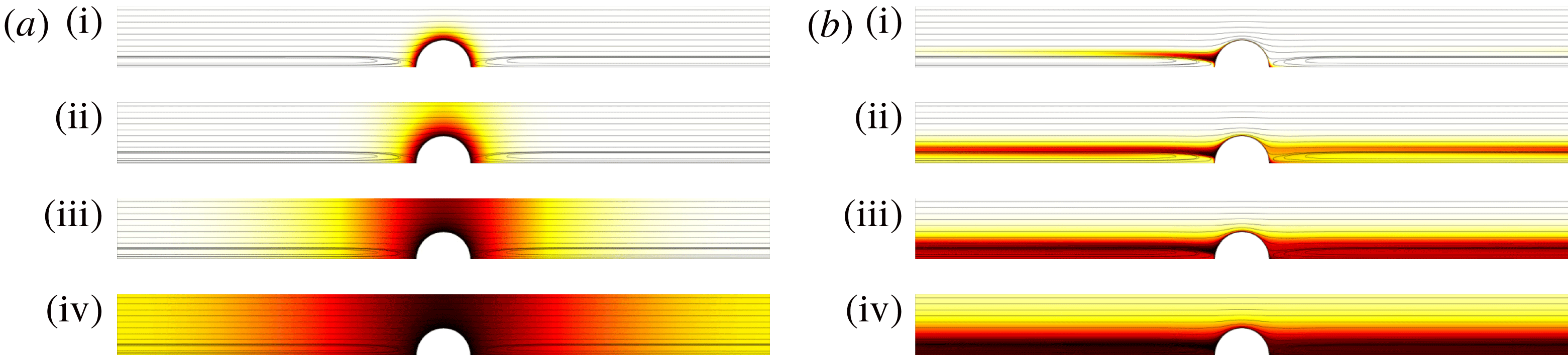
is known, the unsteady advection–diffusion equation (2.8)–(2.11) is solved as depicted in figure 3, together with the streamlines of figure 2. In figure 3(a) we depict the transient for
 $Pe\rightarrow 0$
where we can discern different stages. First, we observe (i) the mass transfer in the radial direction in spherical coordinates attached to the centre of the bubble, until (ii) the penetration length is of the size of the channel radius and the whole cross-section saturates. Then, besides local distortion close to the bubble, (iii) the mass transfer occurs in the axial direction whereas the concentration is uniform in the cross-section. Once the axial penetration length is of the size of half the distance between bubbles, (iv) bubbles interact with each other, establishing an axial concentration field that decays exponentially following a given concentration pattern, i.e. the normalised concentration
 $C(\boldsymbol{x},t)/\overline{C}(t)$
does not change in time.
In figure 3(b) we depict the transient for
 $Pe=10^{5}$
where, again, we can discern different stages. First, we observe (i) the very fast establishment of the boundary layer by diffusion. Then (ii) the fluid convects concentration out of the boundary layer from the divergent stagnation ring and point until it reaches the following bubble which is fed through the convergent stagnation ring and point. Then (iii) the concentration inside the recirculation zone saturates and (iv) it establishes a radial concentration field out of the recirculation zone that decays exponentially following a given concentration pattern, i.e. the normalised concentration
 $C(\boldsymbol{x},t)/\overline{C}(t)$
does not change in time.
Transient evolution of the concentration field
 $C(\boldsymbol{x},t)$
for
 $d=0.45$
,
 $L=12d$
and (a)
 $Pe=0$
or (b)
 $Pe=10^{5}$
. The values of time are (a)
 $t_{\text{(i)}}=4\times 10^{-3}$
,
 $t_{\text{(ii)}}=4\times 10^{-2}$
,
 $t_{\text{(iii)}}=4\times 10^{-1}$
and
 $t_{\text{(iv)}}=2$
, for
 $Pe\rightarrow 0$
as well as (b)
 $t_{\text{(i)}}=2\times 10^{-4}$
,
 $t_{\text{(ii)}}=2\times 10^{-3}$
,
 $t_{\text{(iii)}}=6\times 10^{-3}$
and (d)
 $t_{\text{(iv)}}=3\times 10^{-2}$
, for
 $Pe=10^{5}$
. The axisymmetric concentration field obtained from numerical simulations is represented in colormap where dark red corresponds to saturation concentration and light yellow to the initial concentration. The flow field is represented by the same streamlines as in figure 2.

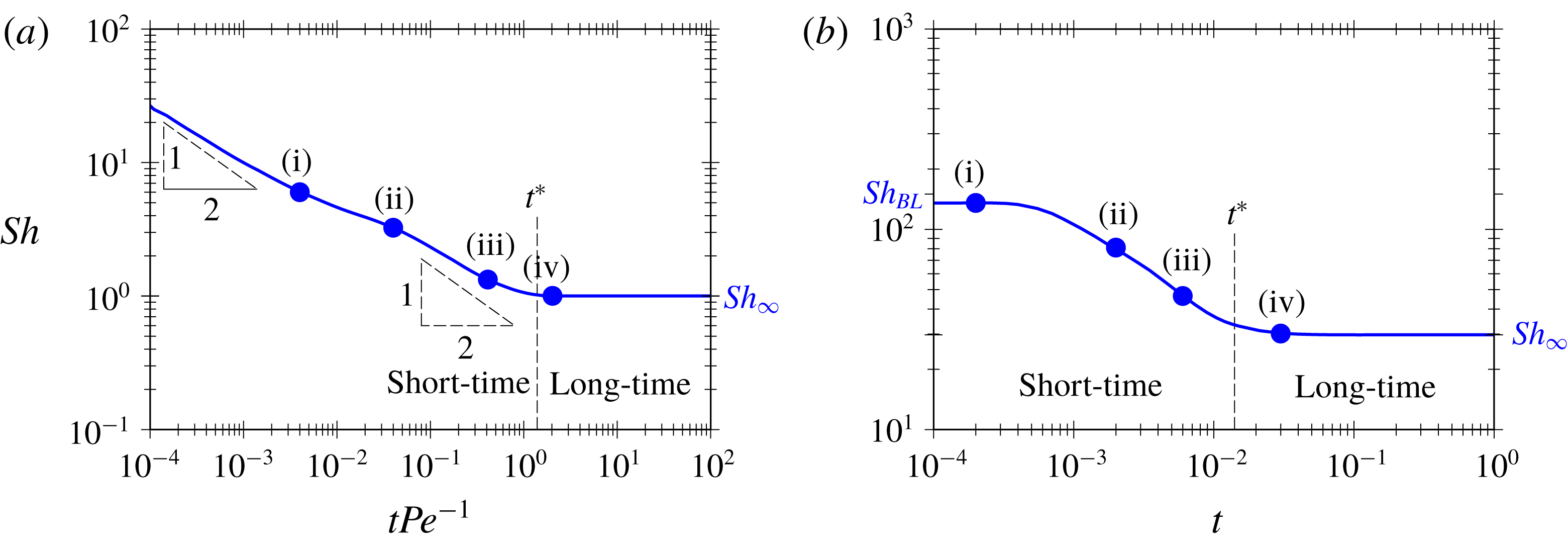
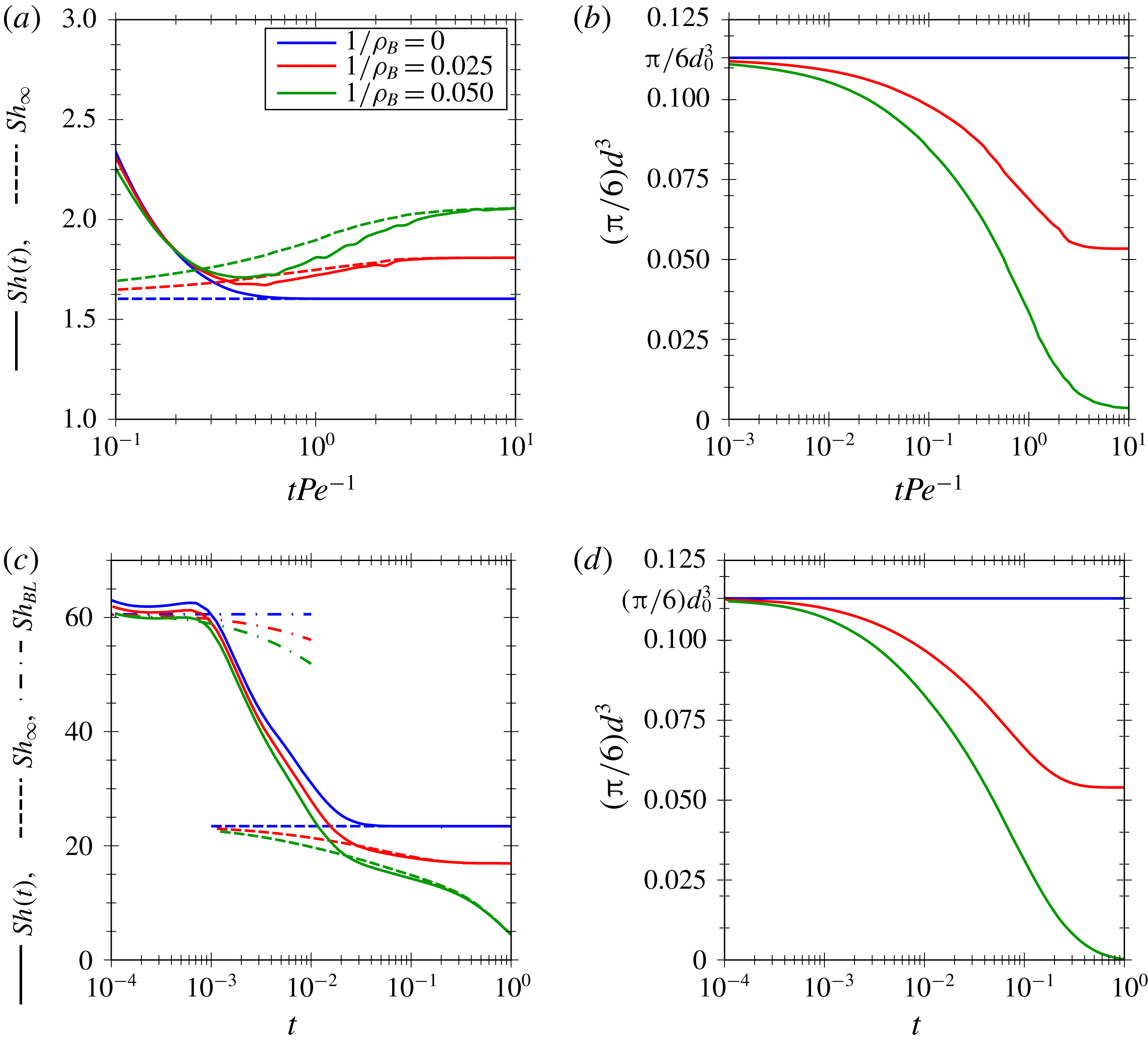
In figure 4, we depict the instantaneous
 $Sh$
number for the two situations considered in figure 3. In both cases, we can observe an initial transient which damps out into a non-vanishing
 $Sh$
number for large time, i.e.
 $Sh_{\infty }=Sh(t\rightarrow \infty )$
. This time-independent value
 $Sh_{\infty }$
is reached for the last stage of the mass transfer when the normalised concentration
 $C(\boldsymbol{x},t)/\overline{C}(t)$
no longer varies in time and then both
 $\overline{C}(t)$
and
 $C(\boldsymbol{x},t)$
, appearing in both sides of (2.12), decay to zero with the same time dependency. The transfer scenario can thus be separated into short- and long-time behaviours,
 $t^{\ast }$
being the threshold which we characterise later in § 5. In the case (a) of short-time behaviour, we observe that, initially, the mass transfer is self-similar in the radial direction in spherical coordinates,
 $C(\boldsymbol{x},t)=\operatorname{erf}[(1/2)(\sqrt{x^{2}+y^{2}+z^{2}}-d/2)t^{-1/2}]$
and the
 $Sh$
number scales approximately as
 $t^{-1/2}$
. Once the penetration length is comparable with the bubble radius (i), the self-similarity solution does not hold exactly, leading to a slight increase of the
 $Sh$
number with respect to the self-similar one due to the change of the curvature of the dissolution front. The penetration length increases in the radial direction in spherical coordinates until it reaches the wall (ii). After this time the penetration length increases only in the axial direction (iii) and the self-similar solution
 $C(\boldsymbol{x},t)=\operatorname{erf}[(1/2)xt^{-1/2}]$
is recovered except in the vicinity of the bubble, which explains the discrepancy with the
 $t^{-1/2}$
trend. Once the bubbles begin to interact (iv), the long-time behaviour establishes. In the case (b) of short-time behaviour, the mass transfer is governed by the boundary layer and the
 $Sh$
number has a constant value
 $Sh_{BL}$
. In this case, the additional mass is stored in the wake (i) which increases until reaching the following bubble (ii). Then the transferred mass is stored in the recirculation zone (iii) and decreases the
 $Sh$
number because mass transfer in the boundary layer inside the recirculation is inhibited. Finally, the long-time behaviour is established (iv), and the mass diffuses radially in cylindrical coordinates. rendering
 $Sh$
constant.
Transient evolution of
 $Sh$
number as a function of time for
 $d=0.45$
,
 $L=12d$
and (a)
 $Pe\rightarrow 0$
or (b)
 $Pe=10^{5}$
.

The independence of the normalised concentration field
 $C(\boldsymbol{x},t)/\overline{C}(t)$
with time in the long-time behaviour suggests eigenmode decomposition of the form
 $$\begin{eqnarray}C(\boldsymbol{x},t)=\mathop{\sum }_{n=1}^{\infty }C_{0,n}\unicode[STIX]{x1D703}_{n}(\boldsymbol{x})\text{e}^{-\unicode[STIX]{x1D70E}_{n}t},\end{eqnarray}$$
where
 $\unicode[STIX]{x1D703}_{n}(\boldsymbol{x})$
,
 $\unicode[STIX]{x1D70E}_{n}$
and
 $C_{0,n}$
are the mass transfer mode, the decay rate whose real part is always positive and the initial amplitude of the
 $n$
th mode ordered such as
 ${\mathcal{R}}e(\unicode[STIX]{x1D70E}_{n})<{\mathcal{R}}e(\unicode[STIX]{x1D70E}_{m})$
for
 $n<m$
. Introducing (3.2) into (2.8)–(2.11) gives the eigenvalue problem
 $$\begin{eqnarray}-\unicode[STIX]{x1D70E}_{n}\unicode[STIX]{x1D703}_{n}+\boldsymbol{v}\boldsymbol{\cdot }\unicode[STIX]{x1D735}\unicode[STIX]{x1D703}_{n}=Pe^{-1}\unicode[STIX]{x1D6FB}^{2}\unicode[STIX]{x1D703}_{n}\quad \text{at }{\mathcal{V}},\end{eqnarray}$$
subject to the boundary conditions
 $$\begin{eqnarray}\displaystyle & \displaystyle \unicode[STIX]{x1D703}_{n}=0\quad \text{at }\unicode[STIX]{x1D6F4}_{B}, & \displaystyle\end{eqnarray}$$
 $$\begin{eqnarray}\displaystyle & \displaystyle \boldsymbol{n}\boldsymbol{\cdot }\unicode[STIX]{x1D735}\unicode[STIX]{x1D703}_{n}=0\quad \text{at }\unicode[STIX]{x1D6F4}_{W}, & \displaystyle\end{eqnarray}$$
 $$\begin{eqnarray}\displaystyle & \displaystyle \unicode[STIX]{x1D703}_{n}(\boldsymbol{x})=\unicode[STIX]{x1D703}_{n}(\boldsymbol{x}+L\boldsymbol{e}_{x})\quad \text{and}\quad \unicode[STIX]{x2202}_{x}\unicode[STIX]{x1D703}_{n}(\boldsymbol{x})=\unicode[STIX]{x2202}_{x}\unicode[STIX]{x1D703}_{n}(\boldsymbol{x}+L\boldsymbol{e}_{x})\quad \text{at }\unicode[STIX]{x1D6F4}_{cross}. & \displaystyle\end{eqnarray}$$
 $\unicode[STIX]{x1D703}_{n}$
the eigenmode and
 $\unicode[STIX]{x1D70E}_{n}$
the eigenvalue. Once the eigenvalue problem is solved, one can obtain the initial amplitudes
 $C_{0,n}$
as done in § 5.
For long time, the concentration field
 $C(\boldsymbol{x},t)$
and its average
 $\overline{C}(t)$
decay exponentially dominated by the slowest mode, as shown by the limits
 $$\begin{eqnarray}\lim _{t\rightarrow \infty }\frac{C(\boldsymbol{x},t)}{\text{e}^{-\unicode[STIX]{x1D70E}_{1}t}}=C_{0,1}\unicode[STIX]{x1D703}_{1}(\boldsymbol{x}),\quad \lim _{t\rightarrow \infty }\frac{\overline{C}(t)}{\text{e}^{-\unicode[STIX]{x1D70E}_{1}t}}=C_{0,1}\overline{\unicode[STIX]{x1D703}}_{1}(\boldsymbol{x}),\end{eqnarray}$$
provided it has a contribution, i.e.
 $C_{0,1}\neq 0$
. The mass transfer is also dominated by the slowest mode. In effect, substituting (3.2) in (2.12) and taking the limit as
 $t$
tends to infinity, the
 $Sh$
number for long time,
 $Sh_{\infty }$
, can be written as
 $$\begin{eqnarray}Sh_{\infty }=\frac{1}{\overline{\unicode[STIX]{x1D703}}_{1}\unicode[STIX]{x03C0}d_{\unicode[STIX]{x1D6F4}}}\int _{\unicode[STIX]{x1D6F4}_{B}}-\boldsymbol{n}\boldsymbol{\cdot }\unicode[STIX]{x1D735}\unicode[STIX]{x1D703}_{1}\,\text{d}\unicode[STIX]{x1D6F4},\end{eqnarray}$$
where
 $Sh_{\infty }$
is independent of the normalisation of the mode. In addition, the normalised concentration field coincides with the slowest mode,
 $$\begin{eqnarray}\lim _{t\rightarrow \infty }C(\boldsymbol{x},t)/\overline{C}(t)=\unicode[STIX]{x1D703}_{1}(\boldsymbol{x})/\overline{\unicode[STIX]{x1D703}}_{1},\end{eqnarray}$$
and therefore
 $Sh_{\infty }$
is independent of time, whereas both the mass transfer and concentration field decay exponentially as
 $\text{e}^{-\unicode[STIX]{x1D70E}_{1}t}$
.
Furthermore, integrating (3.3) for
 $n=1$
over
 ${\mathcal{V}}$
, applying the divergence theorem together with (3.4), and substituting the result in the right-hand side of (3.6), one can relate
 $Sh_{\infty }$
to the decay rate of the first mode,
 $\unicode[STIX]{x1D70E}_{1}$
, as
 $$\begin{eqnarray}Sh_{\infty }=\frac{\unicode[STIX]{x1D70E}_{1}Pe{\mathcal{V}}}{\unicode[STIX]{x03C0}d_{\unicode[STIX]{x1D6F4}}},\end{eqnarray}$$
where
 $\unicode[STIX]{x1D70E}_{1}Pe$
is the decay rate based on the diffusive time scale. Taking the long-time behaviour of the mass transfer
 $\dot{{\mathcal{M}}}_{\infty }$
, the slowest decay becomes dominant and the mass transfer decays in time as
 $$\begin{eqnarray}\dot{{\mathcal{M}}}_{\infty }Pe=\unicode[STIX]{x03C0}d_{\unicode[STIX]{x1D6F4}}Sh_{\infty }C_{0,1}\overline{\unicode[STIX]{x1D703}}_{1}\text{e}^{-\unicode[STIX]{x1D70E}_{1}t}.\end{eqnarray}$$
Since the relation between
 $Sh_{\infty }$
and
 $\unicode[STIX]{x1D70E}_{1}$
is given, the mass transfer in long time is univocally represented by
 $Sh_{\infty }$
. Deriving (3.9) with respect to
 $\unicode[STIX]{x1D70E}_{1}$
, one obtains, using (3.8),
 $$\begin{eqnarray}\frac{\unicode[STIX]{x2202}\dot{{\mathcal{M}}}_{\infty }}{\unicode[STIX]{x2202}\unicode[STIX]{x1D70E}_{1}}={\mathcal{V}}C_{0,1}\overline{\unicode[STIX]{x1D703}}_{1}(1-\unicode[STIX]{x1D70E}_{1}t)\text{e}^{-\unicode[STIX]{x1D70E}_{1}t},\end{eqnarray}$$
which changes sign at
 $t=1/\unicode[STIX]{x1D70E}_{1}$
. This means that an increase in
 $\unicode[STIX]{x1D70E}_{1}$
leads to either an increase or decrease in
 $\dot{{\mathcal{M}}}_{\infty }$
depending on time, for
 $t<1/\unicode[STIX]{x1D70E}_{1}$
and
 $t>1/\unicode[STIX]{x1D70E}_{1}$
, respectively. In addition, the total transferred mass associated to the first mode can be obtained by taking the time integral of
 $\dot{{\mathcal{M}}}_{\infty }$
from
 $0$
to
 $\infty$
in (3.9), leading to
 $\int _{0}^{\infty }\dot{{\mathcal{M}}}_{\infty }\,\text{d}t={\mathcal{V}}C_{0,1}\overline{\unicode[STIX]{x1D703}}_{1}$
, which is independent of
 $\unicode[STIX]{x1D70E}_{1}$
.
It is very important to mention that
 $Sh$
for a short time is dependent on the initial conditions, whereas
 $Sh_{\infty }$
is not.
4 Long-time mass transfer regimes
In this section we study the long-time behaviour and for that purpose we carry out a systematic and exhaustive analysis of the effects of the dimensionless numbers
 $d$
,
 $L$
and, especially,
 $Pe$
on
 $Sh_{\infty }$
for centred and non-deformable bubbles with stress-free interface, with the aim of identifying the different mass transfer regimes.
In figure 5, we schematise the influence of the
 $Pe$
number on the
 $Sh_{\infty }$
number, including representative concentration patterns in the different regimes. We classify these regimes relative to two criteria. The first is the importance of diffusion along the streamlines compared to convection gauged by the magnitude of
 $Pe$
. For small
 $Pe$
numbers, the diffusion along the streamlines is dominant or comparable to convection. For larger
 $Pe$
numbers, convection is dominant as compared to diffusion along the streamlines, which can then safely be neglected. The second criterion is the interaction between bubbles, gauged by the comparison of the magnitude of
 $\tilde{L}$
and any other characteristic convection–diffusion length. If
 $\tilde{L}$
is smaller than or comparable to the relevant convection–diffusion length, bubbles interact and the
 $Sh_{\infty }$
number depends on
 $\tilde{L}$
. If it is larger, no interaction occurs.
Influence of
 $Pe$
on
 $Sh_{\infty }$
for bubbles with stress-free interfaces, diameter
 $d=0.45$
and
 $L=12d$
. Classification of regimes attending to the size of the
 $Pe$
number and the interaction between bubbles. The first mode
 $\unicode[STIX]{x1D703}_{1}$
is represented in colormap where dark red corresponds to saturation
 $\unicode[STIX]{x1D703}_{1}=0$
for given
 $Pe$
number denoted by


In the small
 $Pe$
regimes, there exists a characteristic convection–diffusion length
 $\tilde{\ell }_{CD}\sim \tilde{D}/\tilde{J}$
over which convection and diffusion along the streamlines are of the same order of magnitude. On the one hand, when this distance is larger than the distance between bubbles,
 $\tilde{L}/\tilde{\ell }_{CD}\sim Pe\,\tilde{L}/\tilde{d}_{h}\ll 1$
, diffusion along the streamlines along a distance
 $\tilde{L}$
dominates over convection and then the
 $Sh_{\infty }$
number and the concentration field become independent of
 $Pe$
, i.e. convection is negligible. This regime is named the pure diffusion (PD) regime. On the other hand, when the convection–diffusion length fits between two bubbles,
 $\tilde{L}/\tilde{\ell }_{CD}\sim Pe\,\tilde{L}/\tilde{d}_{h}\gtrsim 1$
, the streamwise diffusion occurs along the distance
 $\tilde{\ell }_{CD}$
, and
 $Sh_{\infty }$
increases with
 $Pe$
as
 $\tilde{\ell }_{CD}/\tilde{d}_{h}\sim Pe^{-1}$
decreases. This regime is named the convection–diffusion (CD) regime. In § 4.1 we characterise these regimes.
In the large
 $Pe$
regimes, diffusion along the streamlines is negligible as compared to convection and the crosswind diffusion becomes crucial. In effect, there appears a boundary layer around the bubble of width
 $\tilde{\ell }_{BL}\sim \sqrt{\tilde{D}\tilde{d}/\tilde{J}}$
, where convection and crosswind diffusion are of the same order of magnitude, together with a wake whose width is of comparable size to the bubble diameter
 $d$
. On the one hand, if the wake length is smaller than the distance between bubbles, the mass transfer occurs mainly in the boundary layer and we name this regime the boundary layer (BL) regime. On the other hand, when the wake length, which increases with the
 $Pe$
number, becomes similar to the distance between bubbles
 $\tilde{L}$
, the mass transfer through the wake becomes dominant as compared to that through the boundary layer, and both concentration pattern and
 $Sh_{\infty }$
number become independent of the
 $Pe$
number. In contrast to the BL regime, the concentration at the streamlines is not determined by the balance between convection and crosswind diffusion, and hence, remains unchanged. For this reason we name this regime the pure convection (PC) regime. In § 4.2 we characterise these regimes. The regime between small and large
 $Pe$
regimes is referred to as the transition (T) regime.
Influence of
 $Pe$
and
 $L$
on
 $Sh_{\infty }$
for bubbles of diameter
 $d=0.45$
.

 $Sh_{BL}$
from figure 4(b).

In figure 6, we depict the influence of the
 $Pe$
number and the distance between bubbles
 $L$
on
 $Sh_{\infty }$
for bubbles of diameter
 $d=0.45$
. We observe that the
 $Sh_{\infty }$
strongly depends on the distance between bubbles in the ‘interacting’ regimes, PD and PC. In particular, we observe that the
 $Sh_{\infty }$
in the PD regime decreases with the length, since axial concentration gradients, represented by the first mode
 $\unicode[STIX]{x1D703}_{1}/\overline{\unicode[STIX]{x1D703}}_{1}$
, are smaller, whereas it increases in the PC regime because of the concomitant increase of the wake length. In the ‘non-interacting’ regimes, CD, T and BL, the characteristic length for the mass transfer is due to the convection–diffusion balance in the streamline and crosswind directions respectively, and hence independent of
 $L$
. It can also be observed that values of
 $Pe$
for which the cross-over between ‘interacting’ and ‘non-interacting’ regimes occurs also depends on
 $L$
. In particular, a decrease in
 $L$
shifts the cross-over value of the
 $Pe$
towards the T regime, eventually making all regimes collapse into a single one as
 $L$
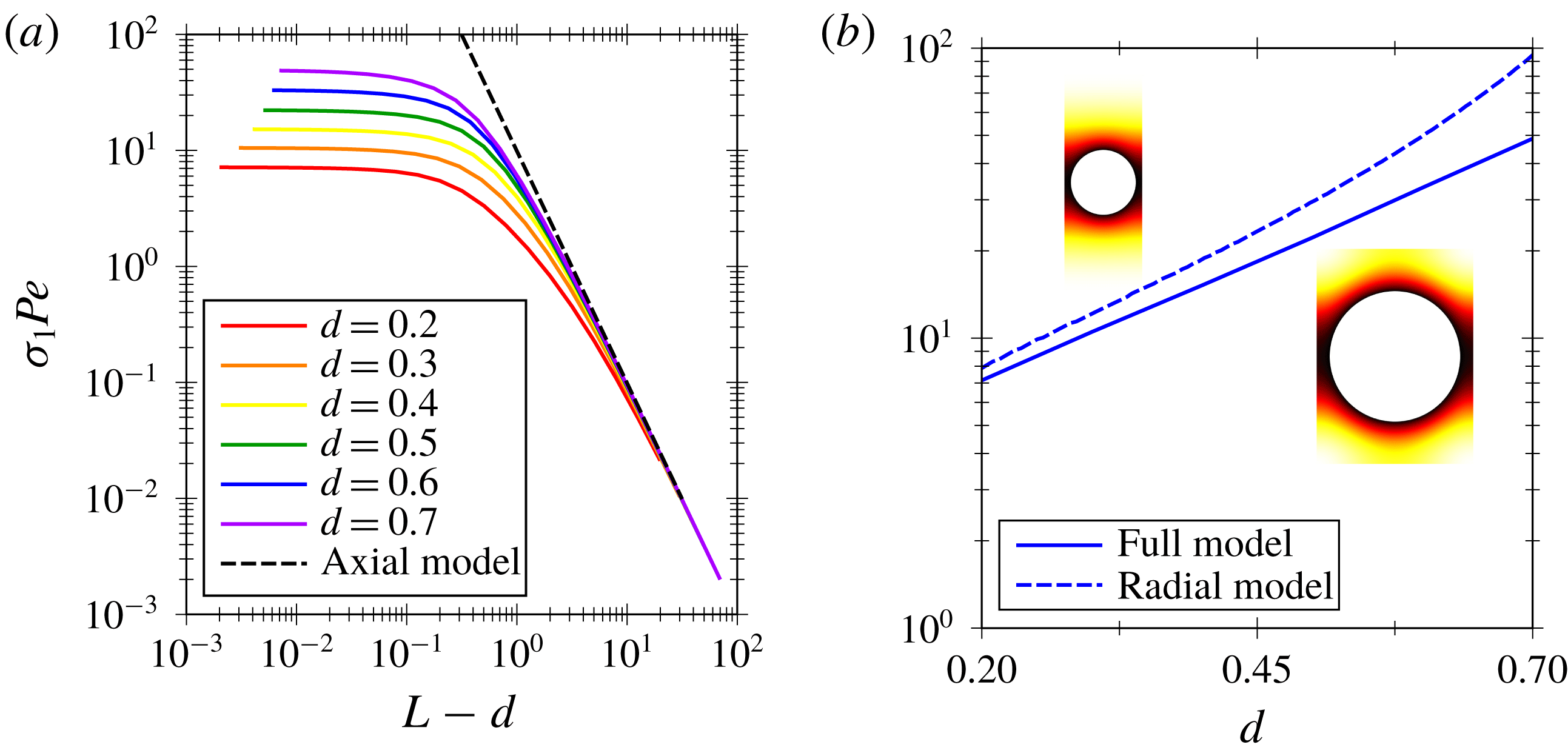
becomes sufficiently small. The system then behaves like a gas cylinder diffusing radially into an annular liquid (see § 4.3). A
 $1/1$
slope emerges for the cross-over between PD and CD regimes, while a
 $1/2$
slope emerges for the BL regime, in agreement with the theory of boundary layers.
 $Sh$
depends on
 $Pe$
as
 $Sh=1+kPe^{\unicode[STIX]{x1D6FC}}$
in an infinite medium (Taylor Reference Taylor1963; Clift Reference Clift1978), where the mass transfer is due to pure radial diffusion for small
 $Pe$
and through a boundary layer for large
 $Pe$
. These two different regimes are analogous to the PD and BL regimes in the present situation. Note that the BL regime does not depend on
 $L$
, whereas the PD does. In an infinite medium, the PD regime is transient and the role of
 $L$
is played by the diffusion length
 $\sqrt{\tilde{D}\tilde{t}}$
. In the case of a confined train of bubbles the dependence of
 $Sh_{\infty }$
on
 $Pe$
is more intricate because of the additional regimes.
It is worth noting that the values of
 $Sh_{\infty }$
shown in figure 4 correspond to the values of
 $Sh_{\infty }$
shown in figure 5. Furthermore, in the transient of the PC regime, the initial
 $Sh_{BL}$
number corresponds to the
 $Sh_{\infty }$
of the BL regime for a bubble of the same size, same
 $Pe$
but
 $L$
sufficiently large to be in the BL regime, as shown in figure 6. This means that the BL regime also describes the short-time behaviour of the PC regime.
4.1 Small
 $Pe$

In this subsection we study both small
 $Pe$
number regimes, PD and CD. For this purpose, we observe that if the distance between bubbles is much larger than the channel diameter,
 $L\gg 1$
, the diffusion is mainly in the axial direction in the far field, i.e. sufficiently far from the bubble, and two-dimensional in the region close to the bubble, i.e. near field. Thus, the concentration is uniform within any cross-section located at
 $x$
except in the vicinity of the bubbles, as quantified later. The mass transfer modes are therefore governed by the one-dimensional counterpart of (3.3) in the axial direction and together with the boundary condition at the bubble surface (3.4a
) and periodicity (3.4c
). Note that (3.4b
) is automatically fulfilled since the mass transfer mode is considered as uniform in the cross-section. In addition, it is worth noting that the convection is imposed by the difference between the mean flow velocity and the velocity of the bubble such that the relevant Péclet number becomes
 $Pe(V-1)$
, whose sign is chosen to be positive. Consequently, if the bubble travels at the mean flow velocity, the mass transfer is purely diffusive. Then the one-dimensional model can be written as
 $$\begin{eqnarray}-\breve{\unicode[STIX]{x1D70E}}_{n}Pe\,\breve{\unicode[STIX]{x1D703}}_{n}-Pe(V-1)\unicode[STIX]{x2202}_{x}\breve{\unicode[STIX]{x1D703}}_{n}=\unicode[STIX]{x2202}_{xx}\breve{\unicode[STIX]{x1D703}}_{n}\quad \text{and}\quad \breve{\unicode[STIX]{x1D703}}_{n}(0)=\breve{\unicode[STIX]{x1D703}}_{n}(L)=0,\end{eqnarray}$$
where
 $\breve{\unicode[STIX]{x1D703}}_{n}(x)$
is the axial mass transfer mode at the cross-section located at
 $x$
and the velocity of the bubble,
 $V$
, is obtained from the hydrodynamics. The domain in this model is the one between two bubbles, which are then located at
 $x=0$
and
 $x=L$
. Although the periodicity (3.4c
) is not imposed, it is automatically fulfilled because of the continuity of the solution. However, in model (4.1) there is a discontinuity of fluxes which is regularised by the near field which is not modelled by (4.1). Model (4.1) is referred to hereafter as the ‘axial model’, as opposed to the ‘full model’ corresponding to (3.3)–(3.4).
The analytical solution of the eigenvalue problem (4.1) is written as
 $$\begin{eqnarray}\breve{\unicode[STIX]{x1D70E}}_{n}Pe\frac{L^{2}}{\unicode[STIX]{x03C0}^{2}}=n^{2}+\left[Pe(V-1)\frac{L}{2\unicode[STIX]{x03C0}}\right]^{2},\quad \breve{\unicode[STIX]{x1D703}}_{n}=\text{e}^{-Pe(V-1)(x/2)}\sin \left(\frac{n\unicode[STIX]{x03C0}x}{L}\right).\end{eqnarray}$$
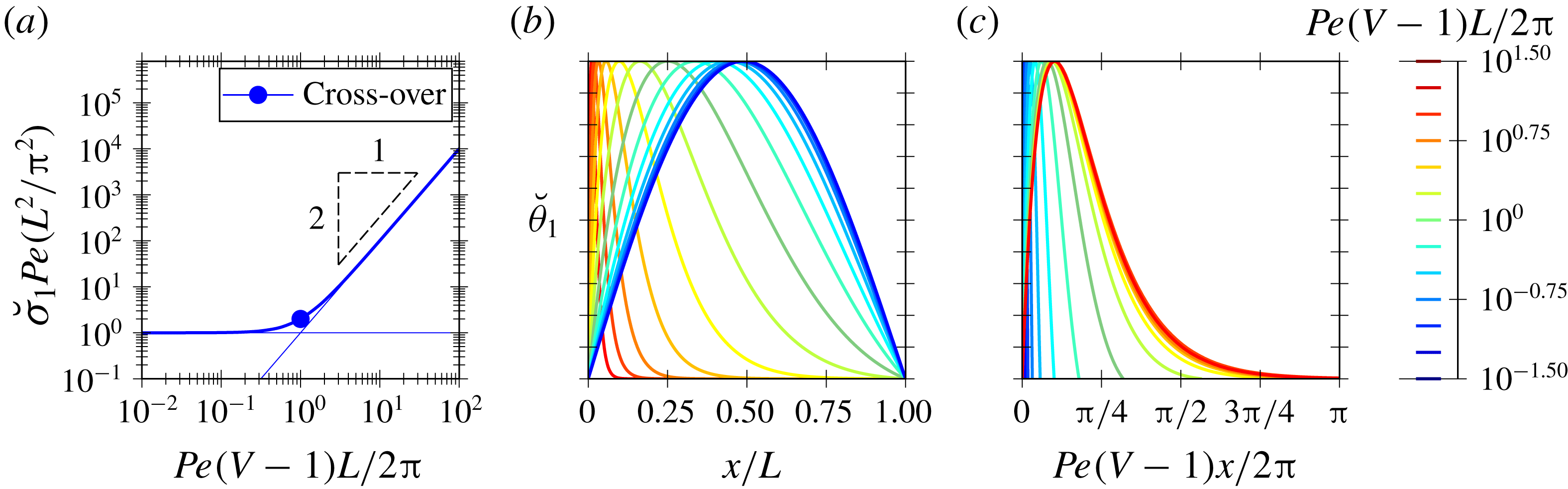
Since the long-time mass transfer is governed by the first mode (3.8), it is depicted for
 $n=1$
in figure 7. The eigenvalue is depicted in figure 7(a) where the cross-over between the PD and CD regimes is marked with

 $Pe(V-1)=2\unicode[STIX]{x03C0}/L$
and
 $\breve{\unicode[STIX]{x1D70E}}_{1}Pe(L^{2}/\unicode[STIX]{x03C0}^{2})=2$
. For large
 $L$
, the volume is approximately
 ${\mathcal{V}}\approx \unicode[STIX]{x03C0}L/4$
and the relation (3.8) between the
 $Sh_{\infty }$
and the eigenvalue
 $\unicode[STIX]{x1D70E}_{1}$
is written as
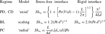
 $(4/\unicode[STIX]{x03C0}^{2})Sh_{\infty }Ld\approx \unicode[STIX]{x1D70E}_{1}Pe(L^{2}/\unicode[STIX]{x03C0}^{2})$
. The eigenmode
 $\breve{\unicode[STIX]{x1D703}}_{1}$
is depicted in figure 7(b–c) conveniently scaling the
 $x$
variable, with either
 $L$
or
 $\ell _{CD}$
, to represent the eigenfunctions in the two regimes, PD or CD, respectively. In the PD regime, which occurs for
 $Pe(V-1)\ll 2\unicode[STIX]{x03C0}/L$
,
 $Sh_{\infty }$
depends on the distance between bubbles as
 $Sh_{\infty }\sim L^{-1}$
. The concentration pattern spans the distance between the bubbles as shown in figure 7(b) and becomes asymmetric due to convection. In contrast, in the CD regime, which occurs in the other limit,
 $Pe(V-1)\gg 2\unicode[STIX]{x03C0}/L$
, the diffusion is concentrated in a region of size
 $x\sim \ell _{CD}\sim Pe^{-1}$
as shown in figure 7(c).
Transition between the PD and CD regimes of the ‘axial model’ (4.1). (a) Eigenvalues and (b,c) eigenmodes represented with two different scalings suitable for PD and CD, respectively.

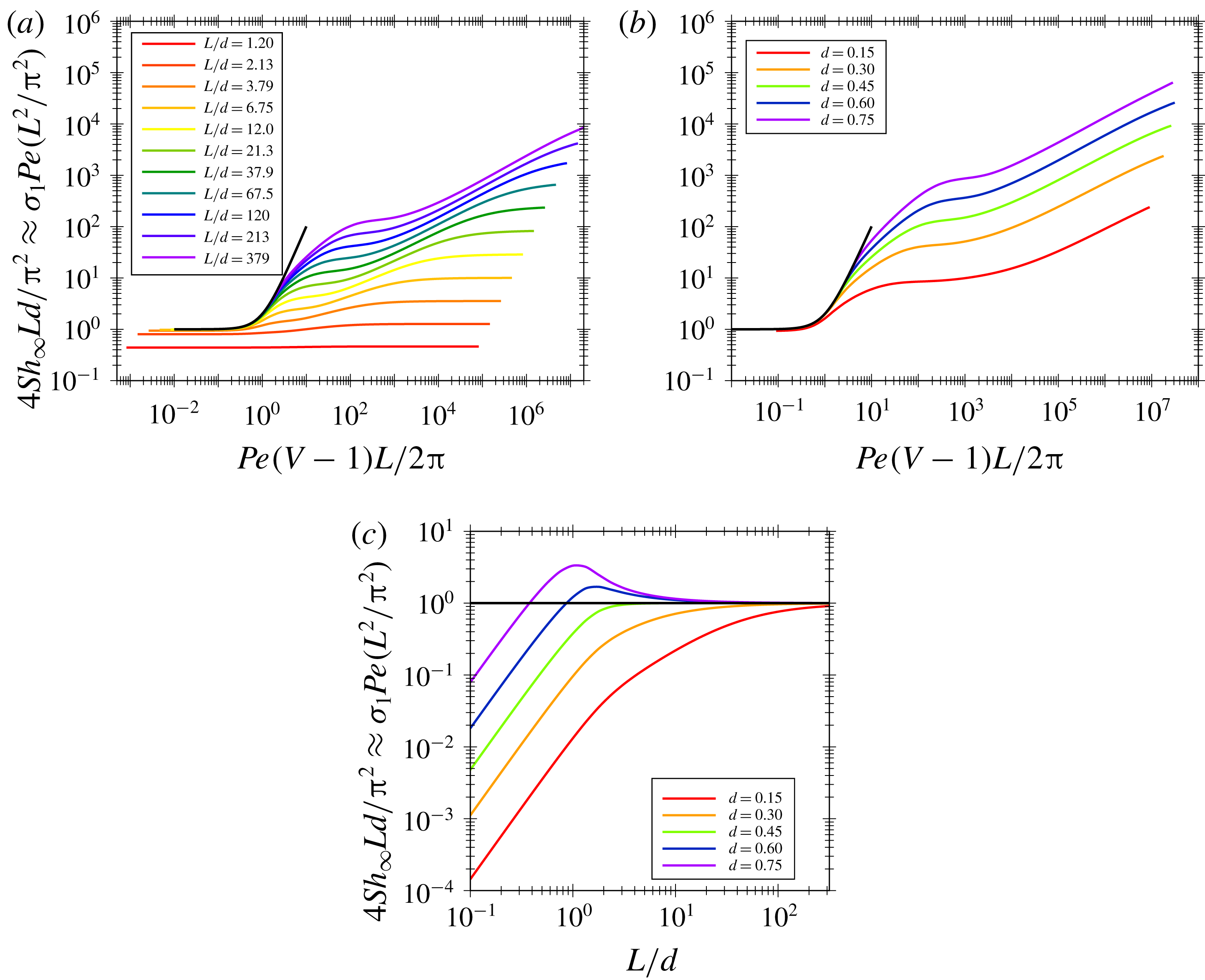
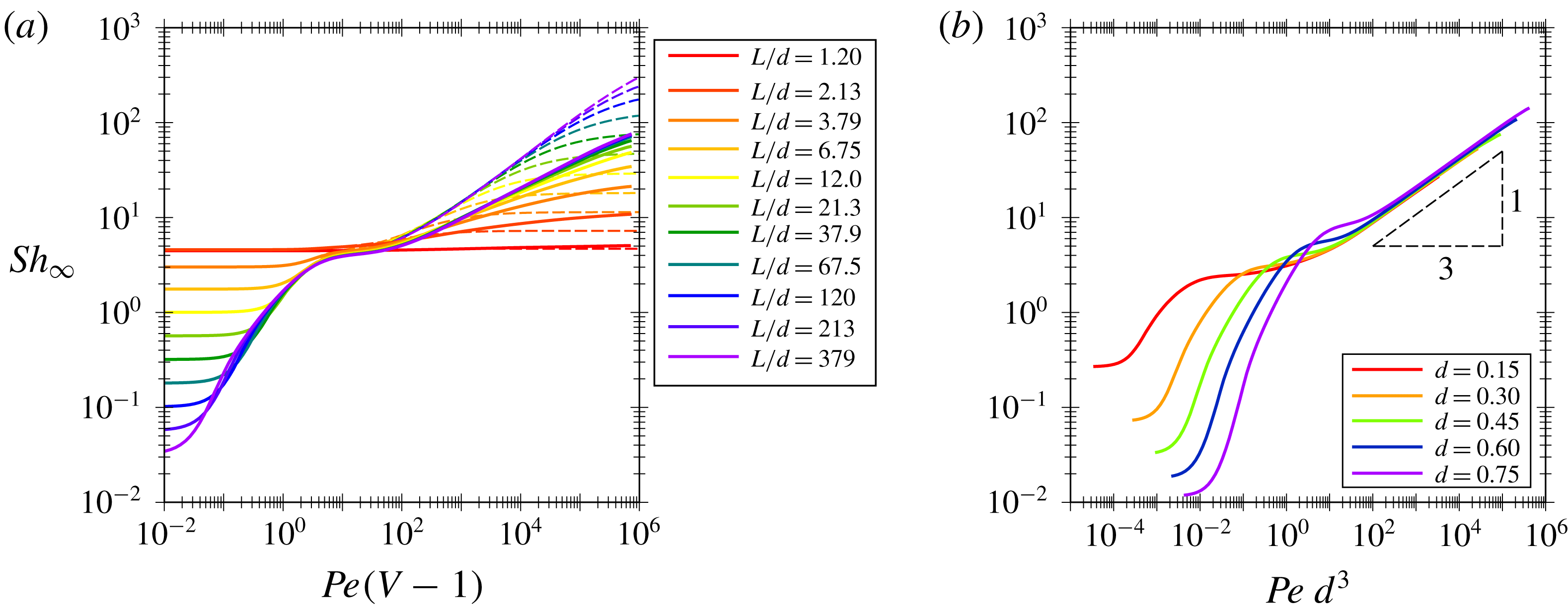
In figure 8 we compare the
 $Sh_{\infty }$
obtained from the ‘axial model’ and the ‘full model’. For this purpose, in figure 8(a) we conveniently rescale the data of figure 6, i.e.
 $Pe$
and
 $Sh_{\infty }$
with
 $(V-1)L/2\unicode[STIX]{x03C0}$
and
 $4Ld/\unicode[STIX]{x03C0}^{2}$
, respectively. In figure 8(a), we can observe that the transition in the small
 $Pe$
regime is governed by the far field, as in the Stokes drag problem, provided
 $L/d$
is sufficiently large, and then is recovered by the ‘axial model’. In figure 8(b) we can observe that, again, the ‘axial model’ is recovered by varying the bubble diameter, hence the bubble velocity. Indeed, the effect of the bubble diameter is considered through the bubble velocity as determined by solving the hydrodynamics, which is reported in our previous work (Rivero-Rodriguez & Scheid Reference Rivero-Rodriguez and Scheid2018a
). In figure 8(c) we observe that the minimum value of
 $L$
to reproduce the ‘axial model’ depends on
 $Pe$
. We observe that the near-field effect is more important for small values of
 $L$
and
 $d$
, whose influence can be either to increase or decrease the mass transfer.
Transition between the PD and CD regimes of the ‘full model’ and —— ‘axial model’ (4.2) for (a) bubbles of diameter
 $d=0.45$
and several distance between bubbles or (b) for distances between bubbles
 $L/d=1.2\times 10^{2.5}$
and several bubble diameters. (c) Influence of
 $d$
and
 $L$
in the PD regime,
 $Pe\rightarrow 0$
.

4.2 Large
$Pe$

In this subsection we study the two large
 $Pe$
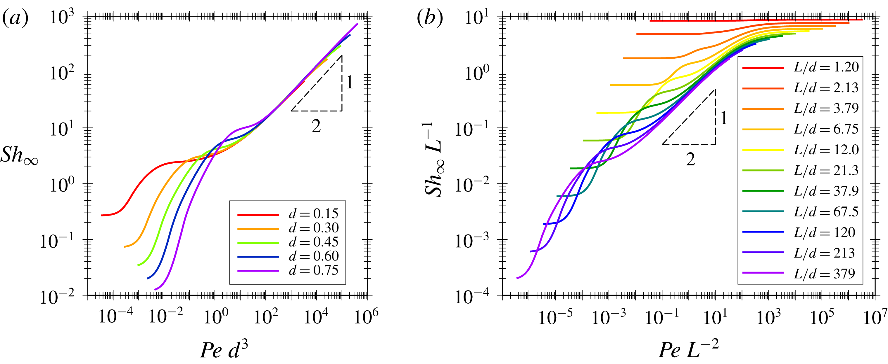
number regimes, BL and PC. In figure 9 we can observe the influence of
 $Pe$
,
 $d$
and
 $L$
on
 $Sh_{\infty }$
and the transition between both regimes. In figure 9(a) we depict the effect of the
 $Pe$
number and bubble size for a sufficiently large distance between bubbles,
 $L=1.2\times 10^{2.5}$
, to have the transition of the PC regime at a larger
 $Pe$
such that
 $Pe=10^{6}$
still lies in the BL regime. For this value of
 $L$
, the BL regime is exhibited for values of
 $Pe$
over a few decades. We can observe a
 $1/2$
slope for the scaling of
 $Sh_{\infty }$
as a function of
 $Pe$
similarly to the case of an infinite medium (Haas, Schmidt-Traub & Brauer Reference Haas, Schmidt-Traub and Brauer1972), which differs from the work by Mikaelian et al. (Reference Mikaelian, Haut and Scheid2015a
) who reported a slope of
 $2/5$
. However, in this model we can observe that the effect of the confinement through the dependency on
 $d$
of
 $Sh_{\infty }$
is by the group
 $Pe\,d^{3}$
which emerges from the balance of convection and diffusion in the BL region. Actually, in shear flows where the velocity is of order
 $\tilde{J}$
and changes within distances of order
 $\tilde{d}$
, such a balance is written as
 $$\begin{eqnarray}\frac{\tilde{J}}{\tilde{d}_{h}}\frac{\tilde{d}}{\tilde{d}_{h}}\sim \frac{\tilde{D}}{\tilde{\unicode[STIX]{x1D6FF}}^{2}},\end{eqnarray}$$
where
 $\tilde{J}/\tilde{d}_{h}$
represents the far-field velocity gradient and
 $\tilde{d}/\tilde{d}_{h}$
represents the change of the velocity in the boundary layer due to the shear that occurs within the direction tangential to the bubble of size
 $\tilde{d}$
, since in the normal direction there is no change of velocity due to the stress-free boundary conditions (2.7), and diffusion occurs within the boundary layer thickness
 $\tilde{\unicode[STIX]{x1D6FF}}$
. Given that
 $\tilde{k}_{\ell }\sim \tilde{D}/\tilde{\unicode[STIX]{x1D6FF}}$
, or equivalently
 $Sh_{\infty }\sim (\tilde{\unicode[STIX]{x1D6FF}}/\tilde{d})^{-1}$
, (4.3) can be rewritten as
 $Sh_{\infty }\sim (Pe\,d^{3})^{1/2}$
.
In figure 9(b) we conveniently rescale the data of figure 6, taking into consideration the
 $1/2$
slope in the BL regime obtained from (4.3), i.e.
 $Pe$
and
 $Sh_{\infty }$
rescaled with
 $L^{-2}$
and
 $L^{-1}$
, respectively. This results in a collapse of the curves for sufficiently large
 $L$
, where we can observe that the transition between the BL and PC regimes occurs for
 $Pe\,L^{-2}\sim 10^{3}$
. For larger values of
 $Pe\,L^{-2}$
, the mass transfer becomes independent of the
 $Pe$
number and depends only on
 $L$
as
 $Sh_{\infty }\sim L$
. This can be explained by the fact that the bubble mainly dissolves radially through the wake whose length is
 $L$
in the PC regime. The small discrepancy might be due to near-field effects close to the bubble, i.e. thicker wakes in this region.
Influence of the
 $Pe$
number on the
 $Sh_{\infty }$
number in regimes with large
 $Pe$
number. (a) Scaling for the BL regime for a large distance between bubbles
 $L/d=1.2\times 10^{2.5}$
and several bubble diameters and (b) transition to the PC regime for a bubble of diameter
 $d=0.45$
, and different lengths
 $L/d$
.

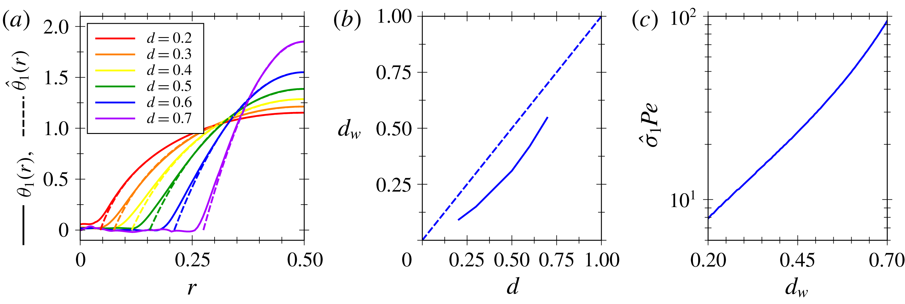
In effect, the concentration pattern in the PC regime is mainly uniform in the axial direction, except in the vicinity of the bubble as shown in figure 5(e). In figure 10(a) we depict the concentration profile of the slowest mode
 $\unicode[STIX]{x1D703}_{1}$
in an arbitrary cross-section far from the bubble where the wake is uniform,
 $r$
being the cylindrical radial coordinate. We can observe that the core of the wake is saturated, i.e.
 $\unicode[STIX]{x1D703}_{1}=0$
, and diffusion is maximal at the contour of the wake of diameter
 $d_{w}$
, decaying as it gets closer to the wall where it vanishes, i.e.
 $-\boldsymbol{n}\boldsymbol{\cdot }\unicode[STIX]{x1D735}\unicode[STIX]{x1D703}_{1}=0$
. The radial counterpart of (3.3)–(3.4), corresponding to uniform velocity and concentration in the axial direction, can be written as
 $$\begin{eqnarray}-\hat{\unicode[STIX]{x1D70E}}_{n}Pe\,\hat{\unicode[STIX]{x1D703}}_{n}=\frac{1}{r}\unicode[STIX]{x2202}_{r}(r\unicode[STIX]{x2202}_{r}\hat{\unicode[STIX]{x1D703}}_{n})\quad \text{and}\quad \hat{\unicode[STIX]{x1D703}}_{n}\left(\frac{d_{w}}{2}\right)=\unicode[STIX]{x2202}_{r}\hat{\unicode[STIX]{x1D703}}_{n}\left(\frac{1}{2}\right)=0,\end{eqnarray}$$
where
 $\hat{\unicode[STIX]{x1D703}}_{n}(r)$
is the radial mass transfer mode at
 $r$
. Model (4.4) is referred to hereafter as the ‘radial model’. The solution of this equation is written as
 $$\begin{eqnarray}\hat{\unicode[STIX]{x1D703}}_{n}(r)=\text{Y}_{0}\left(\sqrt{\hat{\unicode[STIX]{x1D70E}}_{n}Pe}\,\frac{d_{w}}{2}\right)\text{J}_{0}\left(\sqrt{\hat{\unicode[STIX]{x1D70E}}_{n}Pe}\,r\right)-\text{J}_{0}\left(\sqrt{\hat{\unicode[STIX]{x1D70E}}_{n}Pe}\,\frac{d_{w}}{2}\right)\text{Y}_{0}\left(\sqrt{\hat{\unicode[STIX]{x1D70E}}_{n}Pe}\,r\right),\end{eqnarray}$$
where
 $\text{J}_{n}$
and
 $\text{Y}_{n}$
are the Bessel function of the first and second kind and
 $\hat{\unicode[STIX]{x1D70E}}_{n}$
are obtained from the zeros of the expression
 $$\begin{eqnarray}\text{J}_{0}\left(\sqrt{\hat{\unicode[STIX]{x1D70E}}_{n}Pe}\,\frac{d_{w}}{2}\right)\text{Y}_{1}\left(\sqrt{\hat{\unicode[STIX]{x1D70E}}_{n}Pe}\frac{1}{2}\right)-\text{Y}_{0}\left(\sqrt{\hat{\unicode[STIX]{x1D70E}}_{n}Pe}\frac{d_{w}}{2}\right)\text{J}_{1}\left(\sqrt{\hat{\unicode[STIX]{x1D70E}}_{n}Pe}\frac{1}{2}\right)=0.\end{eqnarray}$$
As shown in figure 3(b)(iv), the diameter of the wake
 $d_{w}$
coincides with the diameter of the recirculation region schematised in figure 2. Then the ‘radial model’,
 $\hat{\unicode[STIX]{x1D703}}_{1}$
, reproduces the ‘full model’,
 $\unicode[STIX]{x1D703}_{1}$
, as we show by dashed lines in figure 10(a). The value of
 $d_{w}$
depends on
 $d$
as shown in figure 10(b) where we can see that it is always smaller than
 $d$
. It also corresponds to the size of the wake defined by the width of the recirculating regions shown by the streamlines in figure 5(PC). In figure 10(c) we depict the relation between
 $\hat{\unicode[STIX]{x1D70E}}_{1}Pe$
and
 $d_{w}$
. In effect, the decay rate increases for larger bubbles as
 $d_{w}$
increases with
 $d$
. Since
 $\unicode[STIX]{x1D70E}_{1}Pe$
does not depend on
 $L$
, the
 $Sh_{\infty }$
number, related to
 $\unicode[STIX]{x1D70E}_{1}Pe$
by (3.8), is thus proportional to
 $L$
as chosen in the scaling of the PC regime shown in figure 9(b), i.e.
 $$\begin{eqnarray}Sh_{\infty }(d,L)=\frac{L}{4d}\hat{\unicode[STIX]{x1D70E}}_{1}[d_{w}(d)]Pe.\end{eqnarray}$$
It can be also observed that since the recirculation zone is saturated in the slowest mode, the mass transfer rate at the bubble surface (2.12) is the same as the mass transfer rate at the surface of the recirculation zone. For the latter, the concentration gradient is independent of
 $L$
whereas the surface is proportional to
 $L$
, which explains that
 $Sh_{\infty }\sim L$
in the PC regime as shown in (4.7).
It is worth noting the different dependency of
 $Sh_{\infty }$
on
 $L$
in the different ‘interacting’ regimes, PD and PC, because of the different mechanisms. In the PD regime, the concentration gradient along the axial distance is modified while the bubble surface is kept constant, and thus
 $Sh_{\infty }$
is proportional to
 $L^{-1}$
, whereas in the PC regime, the surface of the recirculation zone is modified while the radial gradient is not affected, and hence
 $Sh_{\infty }$
is proportional to
 $L$
. In both cases, the total transferred mass is independent of
 $Sh_{\infty }$
and proportional to
 ${\mathcal{V}}$
, which increases as
 $L$
increases.
Radial diffusion in the PC regime for
 $L=3$
. (a) Concentration in a cross-section far from the bubble for different bubble diameters. (b) Relation between the bubble diameter and the width of the wake
 $d_{w}$
. (c) Influence of the diameter
 $d_{w}$
on the decay rate
 $\hat{\unicode[STIX]{x1D70E}}_{1}$
.

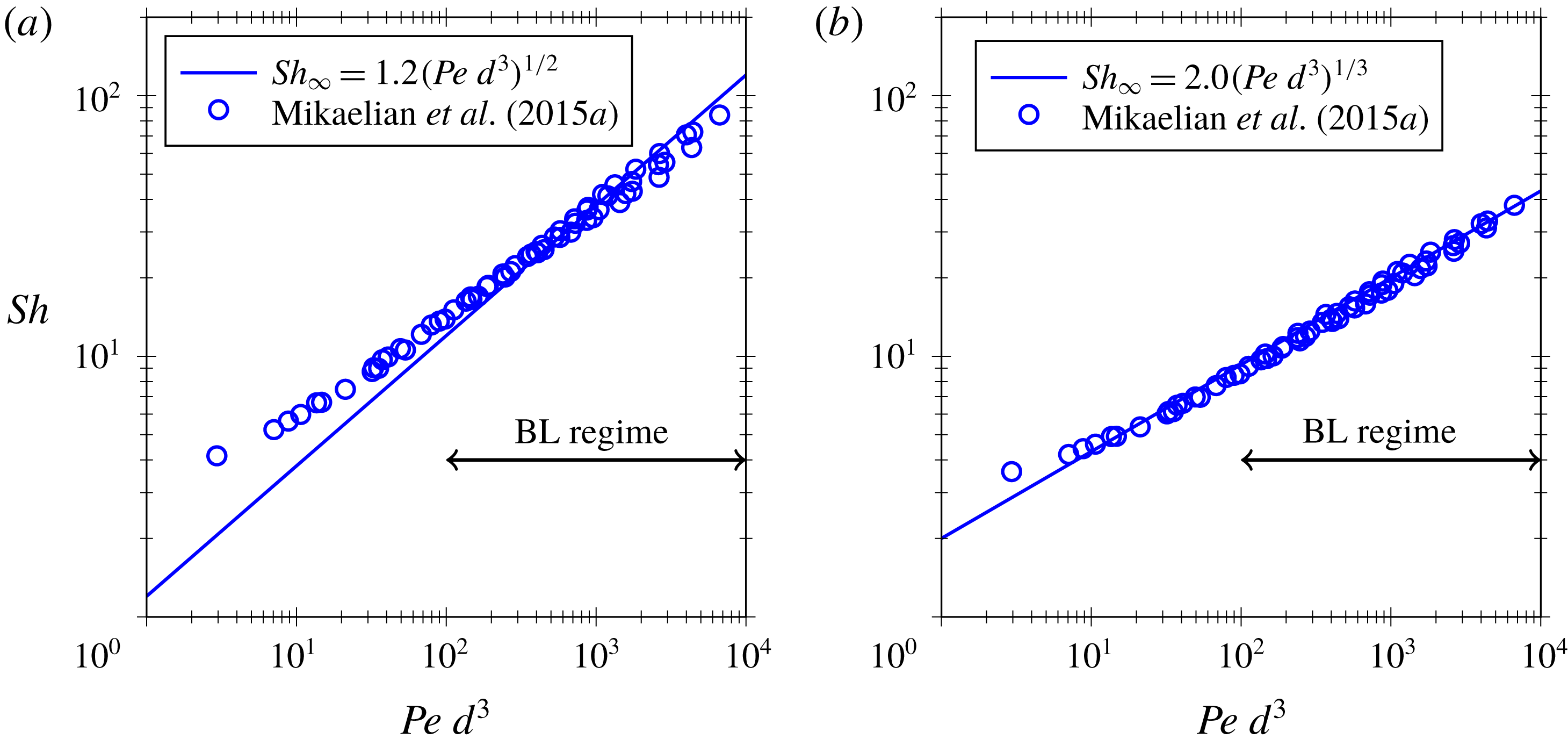
The BL regime was previously studied by Mikaelian et al. (Reference Mikaelian, Haut and Scheid2015a
). Despite the fact that in the model by Mikaelian the mass is steadily advected behind the bubble and in our model the concentration field is periodic and the transferred mass is stored at the liquid in a transient way, there is good agreement between both models in the BL regime, as shown in figure 11. In this figure, we compare our solution in the BL regime with the results of Mikaelian et al. (Reference Mikaelian, Haut and Scheid2015a
). We observe good agreement for large
 $Pe\,d^{3}$
where the bubble is in the BL regime, whereas the power law slightly overestimates the results of Mikaelian et al. (Reference Mikaelian, Haut and Scheid2015a
) for smaller
 $Pe\,d^{3}$
in the T regime, especially for stress-free boundary condition as expected outside the BL regime (see figure 9
a). It also explains the
 $2/5$
power found by Mikaelian et al. (Reference Mikaelian, Haut and Scheid2015a
) by fitting their data in a wider range than the BL regime for which the
 $1/2$
power should rigorously apply in the case of bubbles with stress-free interface. The cross-over between the T regime and the BL regime depends on
 $d$
, and we have identified with a double-arrowed line the region of
 $Pe\,d^{3}$
where the BL regime occurs independently of the value of
 $d$
within the considered range
 $0.15<d<0.75$
.
Comparison with Mikaelian et al. (Reference Mikaelian, Haut and Scheid2015a ) in the BL regime for (a) stress-free and (b) rigid bubble surfaces (see the model extension in § 6.1). Solid lines —— correspond to the best fit in the BL regime of (a) figure 9(a) and (b) figure 15(b).

4.3 Dominating near-field effects: small
$L$

In this subsection we quantify the near-field effects which dominate for small distance between bubbles, i.e.
 $L\sim d$
, already shown in figure 8(c) for the PD regime. We observed in figure 6 that the range of
 $Pe$
for ‘non-interacting’ regimes vanishes for sufficiently small
 $L$
, showing almost no influence of the
 $Pe$
number. Consequently, we can restrict the analysis to the PD regime without loss of generality. In figure 12 we depict the slowest eigenvalue of the full model (3.3)–(3.4) in the PD regime for several diameters and small values of
 $L$
. In figure 12(a) we observe that for sufficiently separated bubbles the ‘axial model’ (4.2) is recovered (dashed line). However, when the size of the gap between bubbles
 $L-d$
is smaller than the bubble diameter, there is no more influence of the distance between bubbles. This is because the diffusion takes place mainly in the radial direction, as happens in the mass transfer of the wake in the PC regime, which leads to very similar
 $Sh_{\infty }$
in both regimes. The effect of the bubble diameter is depicted in figure 12(b), where we observe that
 $\unicode[STIX]{x1D70E}_{1}$
exponentially increases with
 $d$
as
 $\unicode[STIX]{x1D70E}_{1}Pe=\exp (1.1966+3.8318d)$
. In this situation, diffusion occurs at a distance that decreases as the bubble diameter increases, thus
 $\unicode[STIX]{x1D70E}_{1}$
increases. The solution of the ‘radial model’ (4.4), with boundary conditions
 $\hat{\unicode[STIX]{x1D703}}_{n}(d/2)=\unicode[STIX]{x2202}_{r}\hat{\unicode[STIX]{x1D703}}_{n}(1/2)=0$
, is depicted by a dashed line. Examples of the mass transfer modes for small and large bubbles are given in figure 12(b). We observe that for small bubbles the diffusion is mainly radial (cylindrically) since near-field effects are smaller than the distance between the bubble and the wall, thus showing a good agreement with the radial model. However, for large bubbles near-field effects induce axial concentration gradients, increasing the diffusion length and decreasing more significantly the
 $Sh_{\infty }$
number with respect to the ‘radial model’ (4.4).
Near-field effect in the PD regime. Influence on the decay rate of (a) the distance between bubbles for several diameters
 $d$
, and (b)
 $d$
in the limit of small distances
 $L-d\ll 1$
. Two examples of the mass transfer modes are also provided.

5 Short- and long-time contribution to total mass transfer
The maximum transferred mass, i.e. the maximum amount that the liquid can absorb, is
 $\tilde{{\mathcal{M}}}=\tilde{{\mathcal{V}}}(\tilde{C}_{sat}-\tilde{C}_{0})$
, i.e.
 ${\mathcal{M}}={\mathcal{V}}$
in dimensionless form. First, the mass
 ${\mathcal{M}}_{s}$
is transferred in the short-time behaviour and once the faster modes are damped out, the long-time behaviour is established and the rest of the mass
 ${\mathcal{M}}_{\infty }={\mathcal{M}}-{\mathcal{M}}_{s}$
continues to be transferred. We have characterised the
 $Sh$
number for the short-time behaviour in § 3 and for the long-time behaviour in § 4. In this section we investigate the proportion of the total mass transferred by each mode
 $\unicode[STIX]{x1D6F9}_{n}$
, which fulfils
 $\sum _{n=1}^{\infty }\unicode[STIX]{x1D6F9}_{n}=1$
. In particular, we quantify the mass transferred during the short-time behaviour,
 ${\mathcal{M}}_{s}=(1-\unicode[STIX]{x1D6F9}_{1}){\mathcal{M}}$
, and the long-time behaviour,
 ${\mathcal{M}}_{\infty }=\unicode[STIX]{x1D6F9}_{1}{\mathcal{M}}$
.
As in § 3, we assume a uniform initial concentration field (3.1), which, substituted in (3.2) for
 $t=0$
, leads to
 $$\begin{eqnarray}1=\mathop{\sum }_{n=1}^{\infty }C_{0,n}\unicode[STIX]{x1D703}_{n}(\boldsymbol{x}),\end{eqnarray}$$
where
 $C_{0,n}$
can be obtained from the projection of (5.1) onto
 $\unicode[STIX]{x1D703}_{m}$
, already computed and non-orthogonal in general,
 $$\begin{eqnarray}\int _{{\mathcal{V}}}\unicode[STIX]{x1D703}_{m}\,\text{d}{\mathcal{V}}=\mathop{\sum }_{n=1}^{\infty }C_{0,n}\int _{{\mathcal{V}}}\unicode[STIX]{x1D703}_{n}\unicode[STIX]{x1D703}_{m}\,\text{d}{\mathcal{V}},\quad \forall m.\end{eqnarray}$$
Once the initial modal amplitudes
 $C_{0,n}$
are obtained from (5.2), the mean concentration
 $\overline{C}(t)$
can be obtained by averaging (3.2) over the domain
 ${\mathcal{V}}$
as
 $$\begin{eqnarray}\overline{C}(t)=\mathop{\sum }_{n=1}^{\infty }\overline{C}_{0,n}\text{e}^{-\unicode[STIX]{x1D70E}_{n}t},\end{eqnarray}$$
where
 $\overline{C}_{0,n}=C_{0,n}\overline{\unicode[STIX]{x1D703}}_{n}$
is independent of the mode norm
 $\overline{\unicode[STIX]{x1D703}}_{n}$
.
(a) Comparison of faster modes with the slowest one for
 $d=0.45$
and
 $L/d=5$
. (b) Contribution of the first mode to the total transferred mass for a bubble size
 $d=0.45$
.

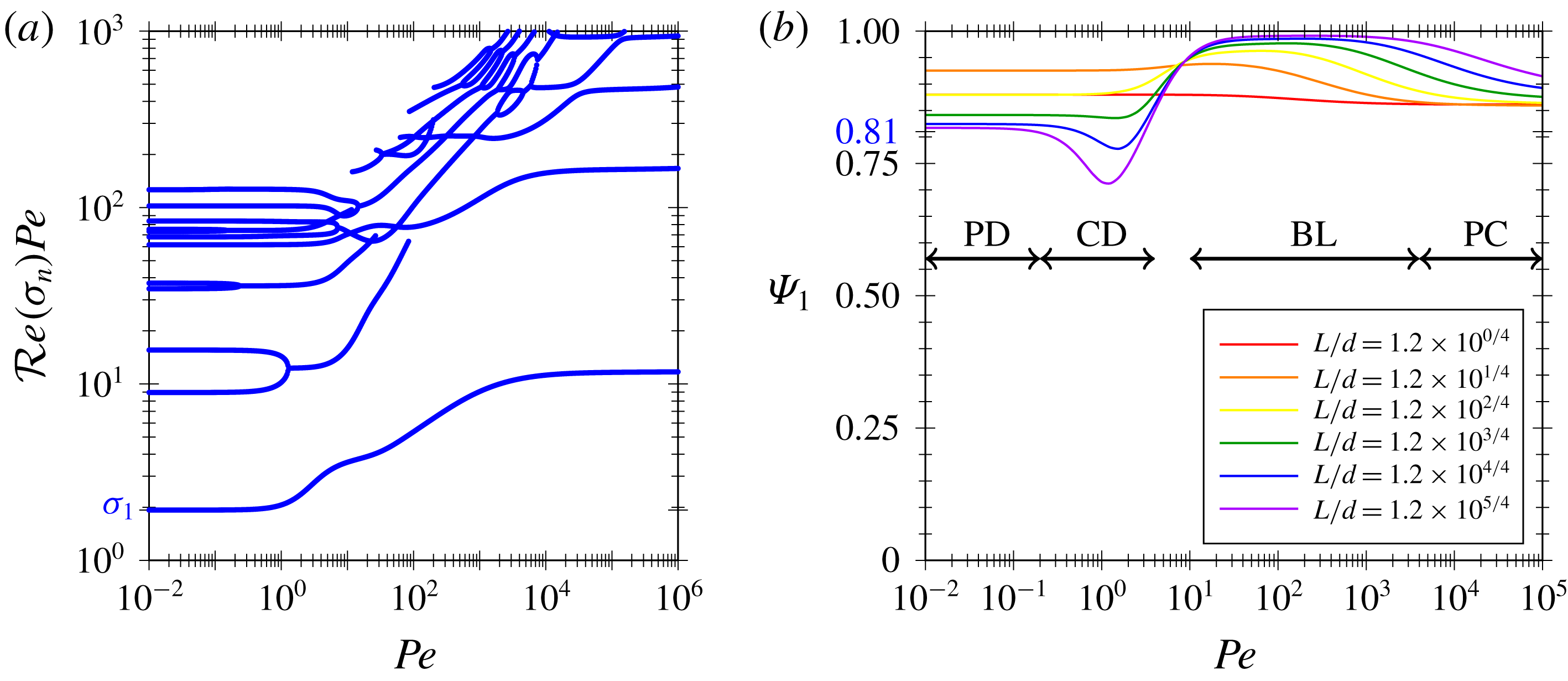
In figure 13(a) we depict the decay rate of faster modes, where we can observe that the contribution of the short-time behaviour, represented by the faster modes
 $\unicode[STIX]{x1D70E}_{n}$
with
 $n>1$
, is much faster than the long-time contribution,
 $\unicode[STIX]{x1D70E}_{1}$
. We can observe that the second slowest decay rate is around one order of magnitude larger, while in the PD regime we consider the third slowest mode for which
 $\unicode[STIX]{x1D70E}_{3}/\unicode[STIX]{x1D70E}_{1}=8.9346$
since the second mode does not contribute to the mass transfer due to the antisymmetry, and in the PC regime
 $\unicode[STIX]{x1D70E}_{2}/\unicode[STIX]{x1D70E}_{1}=14.99$
. The threshold between short and long, previously depicted in figure 3, can be related to the second slowest eigenvalue as
 $t^{\ast }=2/\unicode[STIX]{x1D70E}_{2}$
. During the short-time behaviour, a decay of around 20 %, estimated as
 $1-\text{e}^{-\unicode[STIX]{x1D70E}_{1}t^{\ast }}\approx 1-\text{e}^{-1/5}$
, of the slowest mode occurs. In figure 13(b), we depict the proportion of the total mass transferred in the long run, computed as
 $\unicode[STIX]{x1D6F9}_{1}=\overline{C}_{0,1}$
, and using a sufficiently large basis to obtain results independently of its size, i.e. for
 $n$
up to
 $16$
in this work. It is worth noting that the deviation with respect to unity represents the contribution of the rest of the modes, i.e. during the short-time behaviour. These contributions vary significantly in the different regimes, gauged by the
 $Pe$
number and whose transition depends on
 $L$
, the labels of the regimes in figure 13 being merely indicative.
We can observe that the contribution for the PD and PC regimes does not depend on
 $Pe$
as
 $Sh_{\infty }$
and
 $\unicode[STIX]{x1D703}_{1}$
do not. However, in the CD regime the long-time contribution decreases, as we can see in figure 7(b) that the saturated regions, i.e.
 $\breve{\unicode[STIX]{x1D703}}_{1}=0$
, increase with
 $Pe$
. In the BL regime the saturated region is constrained to the BL region which is small as compared to the total volume and thus
 $\unicode[STIX]{x1D6F9}_{1}$
is almost unity, but slightly increases as the BL gets thinner for larger
 $Pe$
. The transition zone connects the decreasing long-time contribution in the CD zone to the maximal contribution corresponding to the BL regime. For larger
 $Pe$
and as the wake length increases, the long-time contribution decreases down to the value for the PC regime.
Since the PD and PC regimes are well represented by the one-dimensional models, it is possible to obtain the long-time contribution for large
 $L$
. For the PD regime, the solution of the ‘axial model’ is written as
 $\breve{\unicode[STIX]{x1D703}}_{n}(\boldsymbol{x})=\sin (n\unicode[STIX]{x03C0}x/L)$
, and, since
 $\int _{0}^{L}\breve{\unicode[STIX]{x1D703}}_{n}\breve{\unicode[STIX]{x1D703}}_{m}\text{d}x=0$
for
 $n\neq m$
, the modal contribution in the PD regime is written as
 $$\begin{eqnarray}\unicode[STIX]{x1D6F9}_{n}^{PD}=\frac{\displaystyle \left[\int _{0}^{L}\breve{\unicode[STIX]{x1D703}}_{n}\,\text{d}x\right]^{2}}{\displaystyle L\int _{0}^{L}\breve{\unicode[STIX]{x1D703}}_{n}^{2}\,\text{d}x}=4\frac{1-(-1)^{n}}{\unicode[STIX]{x03C0}^{2}n^{2}},\end{eqnarray}$$
where the regime is indicated by the superscript. This vanishes for even values of
 $n$
and for odd ones it yields
 $0.8106$
,
 $0.0900$
,
 $0.0324$
, for
 $n=1$
,
 $n=3$
and
 $n=5$
, respectively. In figure 13(b) it can be observed that the modal contribution of the first mode tends to
 $0.8106$
as
 $L$
increases.
For the PC regime, the ‘radial model’ applies and, since
 $\int _{0}^{L}\hat{\unicode[STIX]{x1D703}}_{n}\hat{\unicode[STIX]{x1D703}}_{m}\text{d}x=0$
for
 $n\neq m$
, the modal contribution in the PC regime is written as
 $$\begin{eqnarray}\unicode[STIX]{x1D6F9}_{1}^{PC}=\frac{\displaystyle \left[\int _{d_{w}/2}^{1/2}\hat{\unicode[STIX]{x1D703}}_{1}\,r\,\text{d}r\right]^{2}}{\displaystyle \frac{1}{8}\,\int _{d_{w}/2}^{1/2}\hat{\unicode[STIX]{x1D703}}_{1}^{2}\,r\,\text{d}r},\end{eqnarray}$$
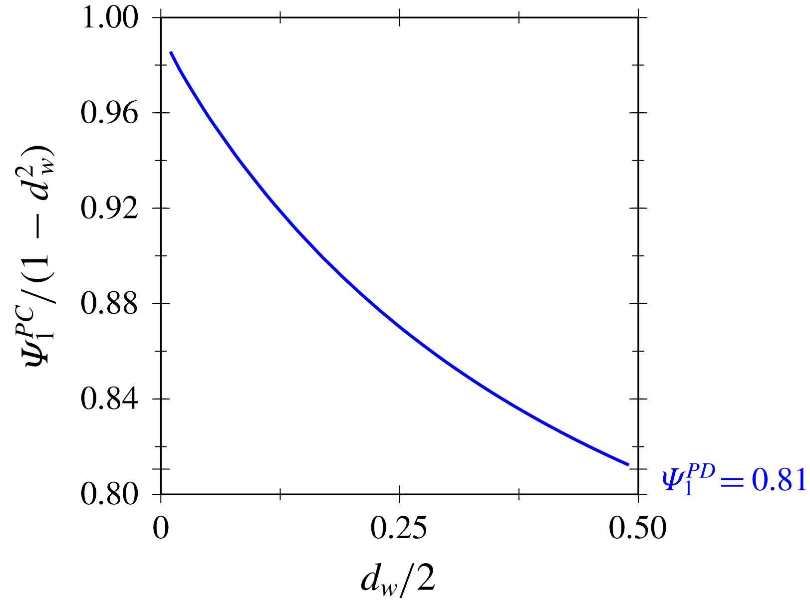
where the regime is indicated by the superscript. Note that only the first mode has no contribution in the recirculation zone and the ‘radial model’ applies. In figure 14, we depict the long-time contribution to the total mass transfer out of the recirculation zone, i.e.
 ${\mathcal{M}}_{\infty }^{PC}/(1-d_{w}^{2})$
, obtained using (5.5). We can observe that the contribution of the first mode out of the recirculation zone is larger for smaller bubbles and remains above
 ${\mathcal{M}}_{\infty }^{PD}$
. This value is attained for bubbles for which the wake diameter
 $d_{w}$
reaches the diameter of the channel, i.e. for which the width of the region out of the recirculation zone is much smaller than the diameter of the channel and the influence of the curvature of the dissolution front becomes negligible.
Modal contribution of the first mode to a uniform initial concentration field in the PC regime obtained from the ‘radial model’ (5.5).

In conclusion, despite the fact that short-time mass transfer is always present, it represents a small proportion of the total mass transfer, and this proportion is minimum for the BL regime, maximum for the PC regime and intermediate for PD and PC regimes as analytically quantified with the axial and the radial models, respectively.
6 Model extensions
In this section we consider some extensions of the hydrodynamic model described in § 2. We study the influence of a rigid interface, the deformability of the bubble, inertial forces and the off-centring of the bubble. The origin of rigid interface can be due to the presence of surfactants in the limit of rigid interface or the substitution of the gas by either a high-viscosity liquid or a solid particle. For further details on the hydrodynamics of the model extensions, the reader is referred to our previous work (Rivero-Rodriguez & Scheid Reference Rivero-Rodriguez and Scheid2018a ).
6.1 Influence of a rigid interface
Tailoring the surface rheology is known to modify the mass transfer, either because of mechanical modification of the surface by adding surfactants (Atasi et al. Reference Atasi, Haut, Pedrono, Scheid and Legendre2018) or solid particles (Beltramo et al. Reference Beltramo, Gupta, Alicke, Liascukiene, Gunes, Baroud and Vermant2017) or because of chemical modification of the mass transfer through the interface. In this subsection we consider the effect of the former in the limit of spherical bubble with rigid interface, which is exhibited in the presence of sufficiently large Marangoni stresses (Atasi et al. Reference Atasi, Haut, Pedrono, Scheid and Legendre2018). For this purpose, the hydrodynamics is governed by (2.2) together with (2.3)–(2.6) and substituting (2.7) by the non-slip condition at the bubble surface,
 $$\begin{eqnarray}\boldsymbol{v}(\boldsymbol{x})=\mathbf{0}\quad \text{at }\unicode[STIX]{x1D6F4}_{B}.\end{eqnarray}$$
It is worth noting that (2.7b ), which is used in the derivation of (3.8), is fulfilled, thus (3.8) also holds in this case.
In figure 15 we depict the influence of
 $Pe$
on
 $Sh_{\infty }$
. First, we compare it with the stress-free case (dashed lines) in figure 15(a). We observe that the small
 $Pe$
regime is not affected by the boundary conditions of the bubble surface, and thus it is also in agreement with the ‘axial model’, which would also describe the PD and CD regimes for other boundary conditions such as those corresponding to viscous droplets or finite Marangoni stresses. Nevertheless, for large
 $Pe$
the mass transfer decreases with respect to the stress-free case due to smaller velocities close to the bubble surface as a consequence of the no-slip condition. In particular, the slope is
 $1/3$
in the BL regime for large
 $L$
as shown in figure 15(b), as already reported by Mikaelian et al. (Reference Mikaelian, Haut and Scheid2015a
) and in general agreement with mass transfer in shear flow (Clift Reference Clift1978). It is worth noting that the interaction of bubbles reduces the slope in the BL regime and makes the PC regime disappear at least in the range of
 $Pe$
considered. In figure 15(b) it can also be observed that in the BL regime,
 $Sh_{\infty }$
depends on
 $d$
proportionally,
 $Sh_{\infty }\sim Pe^{1/3}\,d$
. In effect, in shear flows where the velocity is of order
 $\tilde{J}$
and changes within distances of order
 $\tilde{\unicode[STIX]{x1D6FF}}$
, such a balance is written as
 $$\begin{eqnarray}\frac{\tilde{J}}{\tilde{d}_{h}}\frac{\tilde{\unicode[STIX]{x1D6FF}}}{\tilde{d}_{h}}\sim \frac{\tilde{D}}{\tilde{\unicode[STIX]{x1D6FF}}^{2}},\end{eqnarray}$$
where
 $\tilde{J}/\tilde{d}_{h}$
represents the far-field velocity gradient and
 $\tilde{\unicode[STIX]{x1D6FF}}/\tilde{d}_{h}$
represents the change of the velocity in the boundary layer due to the shear that occurs in the normal direction among the boundary layer thickness
 $\tilde{\unicode[STIX]{x1D6FF}}$
due to the rigid boundary condition (6.1), and diffusion occurs within the boundary layer thickness
 $\tilde{\unicode[STIX]{x1D6FF}}$
. Given that
 $\tilde{k}_{\ell }\sim \tilde{D}/\tilde{\unicode[STIX]{x1D6FF}}$
, or equivalently
 $Sh_{\infty }\sim (\tilde{\unicode[STIX]{x1D6FF}}/\tilde{d})^{-1}$
, (6.2) can be rewritten as
 $Sh_{\infty }\sim (Pe\,d^{3})^{1/3}$
.
In order to understand the interaction between bubbles it is convenient to depict the concentration patterns in the large
 $Pe$
regime. In figure 16, we depict the concentration pattern of bubbles with
 $d=0.5$
, and distance between bubbles
 $L=2$
for different
 $Pe$
numbers. We can observe the strong influence of the flow pattern on the concentration pattern. A mass transfer boundary layer appears with very narrow concentration wakes around the streamlines originating from stagnation points and rings. When wakes extend up to the following bubble, the boundary layers are fed with mass coming from the previous bubble, but the recirculation region is not as saturated as in the case of bubbles with stress-free interface as shown in figure 16(b–e). Consequently, the influence of interaction between bubbles weakens the mass transfer, decreasing
 $Sh_{\infty }$
. It is worth noting that in the case of bubbles with stress-free interfaces, the wakes are of a similar size to the bubble, hence having a stronger impact on the boundary layer. Additionally, the interaction between bubbles does not impose a concentration pattern independently of the
 $Pe$
number as it occurs in the PC regime, at least for the
 $Pe$
numbers considered in the present work.
Influence of the
 $Pe$
number on the
 $Sh_{\infty }$
number for bubbles with rigid interface. (a) Comparison with respect to stress-free bubbles (dashed lines) for diameter
 $d=0.45$
and several
 $L$
. (b) Influence of the diameter for
 $L=379.43d$
.

Streamlines and mass transfer mode
 $\unicode[STIX]{x1D703}_{1}$
(dark red corresponds to saturation
 $\unicode[STIX]{x1D703}_{1}=0$
) in the case of bubbles with rigid interface, diameter
 $d=0.45$
and distance between bubbles
 $L=2$
.

6.2 Influence of a deformable interface
In this subsection we consider the effect of deformable bubbles governed by surface tension. For this purpose, we consider the Young–Laplace contribution for the stress balance in the normal direction. Thus, the hydrodynamics is governed by (2.2) together with (2.3), (2.5), (2.6) and substituting (2.4) and (2.7a ) by the equations for the bubble size and position, i.e.
 $$\begin{eqnarray}\displaystyle & \displaystyle \int _{{\mathcal{V}}_{B}}\text{d}{\mathcal{V}}={\mathcal{V}}_{B}, & \displaystyle\end{eqnarray}$$
 $$\begin{eqnarray}\displaystyle & \displaystyle \int _{{\mathcal{V}}_{B}}\boldsymbol{x}\,\text{d}{\mathcal{V}}=0, & \displaystyle\end{eqnarray}$$
 $$\begin{eqnarray}-p\boldsymbol{n}+\boldsymbol{n}\boldsymbol{\cdot }\unicode[STIX]{x1D749}+p_{G}\boldsymbol{n}=-\frac{1}{Ca}\boldsymbol{n}\unicode[STIX]{x1D735}\boldsymbol{\cdot }\boldsymbol{n}\quad \text{at }\unicode[STIX]{x1D6F4}_{B},\end{eqnarray}$$
where
 $p_{G}$
is the pressure of the gas. In (6.4),
 $Ca=\tilde{\unicode[STIX]{x1D707}}\tilde{J}/\tilde{\unicode[STIX]{x1D6FE}}$
is the capillary number. This system of equations is solved using the boundary arbitrary Lagrangian–Eulerian method developed by Rivero-Rodriguez, Perez-Saborid & Scheid (Reference Rivero-Rodriguez, Perez-Saborid and Scheid2018) for the solution of partial differential equations on deformable domains, and outlined in appendix A.
Influence of the deformability of bubbles, as gauged by
 $Ca$
for bubbles with diameter
 $d=0.45$
and distance between bubbles
 $L=12d$
, on (a) the
 $Sh_{\infty }$
number and (b) the bubble surface.

In figure 17 we plot the influence of the deformability of the bubble gauged by the
 $Ca$
number. In figure 17(a) the influence of
 $Ca$
number for the different regimes is depicted, conveniently scaling the
 $Pe$
number by the relative flow velocity
 $V-1$
. We observe that the
 $Sh_{\infty }$
number does not depend on
 $Ca$
except in the PC regime. It is worth noting that the surface of the bubble
 $\unicode[STIX]{x1D6F4}_{B}$
and its equivalent diameter
 $d_{\unicode[STIX]{x1D6F4}}$
, on which the mass transfer coefficient and
 $Sh_{\infty }$
numbers are based, as well as the velocity of the bubble significantly depend on the
 $Ca$
number and volume of the bubble,
 ${\mathcal{V}}_{B}=\unicode[STIX]{x03C0}d^{3}/6$
, as depicted in figure 17(b), respectively. The bubble surface increases (see figure 17
b) as well as the velocity of the bubble which can even increase above the maximum velocity of the Poiseuille flow for sufficiently large
 $Ca$
as already shown in our previous work (Rivero-Rodriguez & Scheid Reference Rivero-Rodriguez and Scheid2018a
), i.e.
 $V>2$
. It is worth noting that the deformable case reduces, for
 $Ca\rightarrow 0$
, to the bubble with stress-free spherical interface.
Streamlines and mass transfer mode
 $\unicode[STIX]{x1D703}_{1}$
(dark red corresponds to saturation
 $\unicode[STIX]{x1D703}_{1}=0$
) for deformable bubbles with
 $d=0.5$
,
 $L=1.5$
and in the PC regime, with
 $Pe=10^{5}$
.

To understand the influence of
 $Ca$
in the PC regime, we depict the concentration pattern in this regime in figure 18. We can observe how bubbles and wakes stretch as
 $Ca$
increases. Since we have seen that
 $Sh_{\infty }$
diminishes in the PC regime when wakes stretch,
 $Sh_{\infty }$
thus diminishes as
 $Ca$
increases.
6.3 Influence of inertia
In this subsection we study the effect of inertia in the mass transfer around the bubble. To consider inertia, the hydrodynamics is governed not by the Stokes equations (2.2), but by the Navier–Stokes equations
 $$\begin{eqnarray}\displaystyle & \displaystyle \unicode[STIX]{x1D735}\boldsymbol{\cdot }\boldsymbol{v}=0\quad \text{at }{\mathcal{V}}, & \displaystyle\end{eqnarray}$$
 $$\begin{eqnarray}\displaystyle & \displaystyle Re\,\boldsymbol{v}\boldsymbol{\cdot }\unicode[STIX]{x1D735}\boldsymbol{v}=-\unicode[STIX]{x1D735}p+\unicode[STIX]{x1D735}\boldsymbol{\cdot }\unicode[STIX]{x1D749}\quad \text{at }{\mathcal{V}}, & \displaystyle\end{eqnarray}$$
 $Re=\tilde{\unicode[STIX]{x1D70C}}\tilde{J}\tilde{d}_{h}/\tilde{\unicode[STIX]{x1D707}}$
is the Reynolds number, together with (2.3)–(2.7).
After simulations for
 $Re$
up to
 $100$
, we observed that changes in the hydrodynamics have no influence on
 $Sh_{\infty }$
within a
 $1\,\%$
error. This is due to the fact that for small
 $Pe$
the system behaviour is well described by the ‘axial model’ which only considers the effect of the hydrodynamics through the velocity of the bubble. In regimes with large
 $Pe$
, the Schmidt number
 $Sc=\unicode[STIX]{x1D707}/(D\unicode[STIX]{x1D70C})$
is much larger than unity,
 $Sc\gg 1$
. Thus, the viscous boundary layer is much thicker than the diffusive one, and hence the details of the viscous boundary layers tuned by the
 $Re$
do not affect the diffusive one.
Thus, the influence of inertia is through the inertial migration force, responsible for the off-centre position of the bubbles. This effect was first reported by Segré & Silberberg (Reference Segré and Silberberg1962). In the next subsection we consider the effect of off-centred positions of the bubble on the mass transfer.
6.4 Effect of off-centred positions
In our recent work (Rivero-Rodriguez & Scheid Reference Rivero-Rodriguez and Scheid2018a
), the equilibrium positions of deformable bubbles and rigid particles in inertial flows in the presence of an outer uniform force as a function of the diameter and the
 $Re$
and the
 $Ca$
numbers are reported. In this subsection we consider the effect on mass transfer of off-centred positions of the bubble,
 $\unicode[STIX]{x1D700}$
, measured from the centre of the microchannel. In the case of stress-free bubbles the governing equations remain the same. However, in the case of rigid spheres in an off-centred position, the velocity at the bubble interface (6.1) is modified as
 $$\begin{eqnarray}\displaystyle & \displaystyle \boldsymbol{v}(\boldsymbol{x})=\unicode[STIX]{x1D734}\times (\boldsymbol{x}-\unicode[STIX]{x1D73A})\quad \text{at }\unicode[STIX]{x1D6F4}_{B}, & \displaystyle\end{eqnarray}$$
 $$\begin{eqnarray}\displaystyle & \displaystyle \mathbf{0}=\int _{\unicode[STIX]{x1D6F4}_{B}}\boldsymbol{n}\boldsymbol{\cdot }\unicode[STIX]{x1D749}\times (\boldsymbol{x}-\unicode[STIX]{x1D73A})\,\text{d}\unicode[STIX]{x1D6F4}, & \displaystyle\end{eqnarray}$$
 $\unicode[STIX]{x1D734}$
is the rotational velocity of the bubble which results in moment equilibrium, and
 $\unicode[STIX]{x1D73A}=\unicode[STIX]{x1D700}\boldsymbol{e}_{y}$
.
In figure 19 we plot the influence of off-centred positions for bubbles with both stress-free and rigid interfaces. On the one hand, we can observe that in regimes with small
 $Pe$
the
 $Sh_{\infty }$
is affected by the eccentricity through the velocity of the bubble. On the other hand, the velocity field slightly affects the
 $Sh_{\infty }$
in the regime with large
 $Pe$
. In particular, the effect on bubbles with stress-free interfaces is non-monotonic. For bubbles with rigid interface the effect is monotonic, tending to decrease the slope and even revealing the PC regime for large
 $Pe$
in the range of
 $Pe$
considered.
Effect on
 $Sh_{\infty }$
of the off-centre position for bubbles with diameter
 $d=0.45$
and distance between bubbles
 $L=20d$
. (a) Stress-free and (b) rigid interfaces.

In figure 20, we can observe the influence of the eccentricity
 $\unicode[STIX]{x1D700}$
on the flow structure and hence on the mass transfer modes, which we depicted in the region with large
 $Pe$
number,
 $Pe=10^{4}$
. We can observe how the stagnation regions, either points or lines, detach from the bubble surface. Observe that the divergent stagnation points/lines extract concentration from the boundary layer at the bubble surface. This intricate effect on the hydrodynamics might explain the non-monotonicity of the mass transfer, which makes it difficult to quantify by analytical means.
Streamlines and mass transfer mode
 $\unicode[STIX]{x1D703}_{1}$
(dark red corresponds to saturation
 $\unicode[STIX]{x1D703}_{1}=0$
) in the case of bubbles with stress-free interface, diameter
 $d=0.45$
, distance between bubbles
 $L=20d$
and
 $Pe=10^{4}$
.

7 Discussion on dissolution
In this section the dissolution of a train of bubbles is investigated. For this purpose, the previous model for the mass transfer is extended to take into account the change in size of the bubble. First, we discuss the different scenarios regarding the steady state, being either (i) complete dissolution when the bubble is fully dissolved or (ii) partial dissolution when the liquid saturates before the full dissolution occurs and bubbles of given size remain. Secondly, we investigate the transient behaviour and compare
 $Sh(t)$
with
 $Sh_{\infty }$
to quantify the fact that the quasi-steadiness assumption does not strictly hold because the mass transfer and the change in size of the bubble take place on the same time scale. The concentration and density are made dimensionless with
 $\tilde{C}_{sat}-\tilde{C}_{0}$
.
7.1 Steady state
Different scenarios arise depending of the comparison between the amount of gas that the liquid can potentially absorb,
 $\tilde{{\mathcal{V}}}(\tilde{C}_{sat}-\tilde{C}_{0})$
, which is written as
 ${\mathcal{V}}$
in dimensionless form, and the initial amount of gas in the bubble,
 $\unicode[STIX]{x1D70C}_{B}(\unicode[STIX]{x03C0}/6)d_{0}^{3}$
, available for dissolution,
 $\unicode[STIX]{x1D70C}_{B}=\tilde{\unicode[STIX]{x1D70C}}_{B}/(\tilde{C}_{sat}-\tilde{C}_{0})$
being the dimensionless counterpart of the density of the gas inside the bubble,
 $\tilde{\unicode[STIX]{x1D70C}}_{B}$
, and
 $d_{0}$
its dimensionless initial diameter. On the one hand, if the liquid cannot absorb all the gas,
 $\unicode[STIX]{x1D70C}_{B}(\unicode[STIX]{x03C0}/6)d_{0}^{3}>{\mathcal{V}}$
, there is partial dissolution and the amount
 $\unicode[STIX]{x1D70C}_{B}(\unicode[STIX]{x03C0}/6)d_{0}^{3}-{\mathcal{V}}$
will remain undissolved in a bubble of size
 $d(t\rightarrow \infty )/d_{0}=\sqrt[3]{1-{\mathcal{V}}/(\unicode[STIX]{x1D70C}_{B}(\unicode[STIX]{x03C0}/6)d_{0}^{3})}$
. The amount
 ${\mathcal{V}}$
dissolves first according to the short-time behaviour by an amount
 $(1-\unicode[STIX]{x1D6F9}_{1}){\mathcal{V}}$
and then according to the long-time behaviour by an amount
 $\unicode[STIX]{x1D6F9}_{1}{\mathcal{V}}$
. During the short-time behaviour, a small portion of
 $\unicode[STIX]{x1D6F9}_{1}{\mathcal{V}}$
is also dissolved. On the other hand, if the liquid can absorb all the gas, the dissolution is complete and bubbles vanish. In figure 21 we schematise this process. The symbol ● represents the initial conditions, and the vertical line from 0 to
 $\unicode[STIX]{x1D70C}_{B}(\unicode[STIX]{x03C0}/6)d_{0}^{3}$
represents the initial amount of gas in the bubble. This amount is the total amount of undissolved and dissolved gas. The latter can be divided in short- and long-time behaviour. If the operating conditions are below the complete–incomplete dissolution line
 $\cdot$
–
 $\cdot$
–, the bubble completely dissolves. If the operating conditions are within the short-time region, only short-time dissolution matters. However, this is only found for gas with high solubility,
 $\unicode[STIX]{x1D70C}_{B}(\unicode[STIX]{x03C0}/6)d_{0}^{3}<(1-\unicode[STIX]{x1D6F9}_{1}){\mathcal{V}}$
. The threshold for partial or complete dissolution is
 $\unicode[STIX]{x1D70C}_{B}(\unicode[STIX]{x03C0}/6)d_{0}^{3}={\mathcal{V}}$
, whereas the threshold for short- and long-time dissolution is
 $\unicode[STIX]{x1D70C}_{B}(\unicode[STIX]{x03C0}/6)d_{0}^{3}=(1-\unicode[STIX]{x1D6F9}_{1}){\mathcal{V}}$
.
Map on the dissolution process. After the dissolution process, the amount
 $\unicode[STIX]{x1D70C}_{B}\frac{\unicode[STIX]{x1D70B}}{6}d_{0}^{3}-{\mathcal{V}}$
remains undissolved, the amount
 $\unicode[STIX]{x1D6F9}_{1}{\mathcal{V}}$
dissolves in the long-time behaviour and the amount
 $(1-\unicode[STIX]{x1D6F9}_{1}){\mathcal{V}}$
dissolves in the short-time behaviour.

It is worth noting that for
 $\unicode[STIX]{x1D70C}_{B}(\unicode[STIX]{x03C0}/6)d_{0}^{3}>{\mathcal{V}}$
, bubbles do not completely dissolve through the mechanism studied in this work, especially for a finite train length for which there is a collective dissolution behaviour (Michelin, Guérin & Lauga Reference Michelin, Guérin and Lauga2018) such as the gas diffuses in the liquid out of the train of bubbles. This collective mode is much slower than that presented in this work since the distance that the gas needs to be transported becomes much longer and of the order of the bubble train. An increase in the distance between bubbles can lead to a decrease or increase in the
 $Sh$
number in the PD and PC regimes, respectively, and has no influence on the other regimes. In addition, it is associated with an increase in
 ${\mathcal{V}}$
and hence a decrease in
 $\unicode[STIX]{x1D70C}_{B}(\unicode[STIX]{x03C0}/6)d_{0}^{3}-{\mathcal{V}}$
, and it might lead to an increment of the undissolved amount of gas which remains to be dissolved in the collective mode. For instance, in the PD regime, it initially leads to a faster saturation of the liquid inside the train, decreasing the dissolved amount and an increment of the amount to be dissolved in the collective mode. It thus yields a large increment of the total dissolution time.
Influence of bubble size changes in the (a,b) PD regime for
 $Pe\rightarrow 0$
and (c,d) PC regime,
 $Pe=10^{4}$
, for
 $d_{0}=0.6$
and
 $L_{0}=3$
.
 $(\unicode[STIX]{x03C0}/6)d^{3}/{\mathcal{V}}=0.050\,42$
.

7.2 Transient dissolution
Although in many situations the change in size is very small as compared to its initial value as
 ${\mathcal{V}}\ll \unicode[STIX]{x1D70C}_{B}(\unicode[STIX]{x03C0}/6)d_{0}^{3}$
, changes in bubble size can be important. Nonetheless, its effect might be limited, as shown in what follows. To study its influence on the dissolution process, changes in bubble size must be taken into account. For this purpose, the mass balance of gas is applied:
 $$\begin{eqnarray}\frac{\unicode[STIX]{x2202}(\unicode[STIX]{x1D70C}_{B}\frac{4}{3}\unicode[STIX]{x03C0}d^{3})}{\unicode[STIX]{x2202}t}=-\dot{{\mathcal{M}}},\quad d(0)=d_{0},\end{eqnarray}$$
Since
 $(1/4)\unicode[STIX]{x03C0}L(t)={\mathcal{V}}+(4/3)\unicode[STIX]{x03C0}d^{3}(t)$
and the volume
 ${\mathcal{V}}$
does not change in time, the distance between bubbles can be obtained from
 $$\begin{eqnarray}\frac{\unicode[STIX]{x2202}\left(\unicode[STIX]{x03C0}L/4\right)}{\unicode[STIX]{x2202}t}=-\frac{\dot{{\mathcal{M}}}}{\unicode[STIX]{x1D70C}_{B}},\quad L(0)=L_{0},\end{eqnarray}$$
where
 $L_{0}$
is the initial distance between bubbles. In addition,
 $C_{sat}$
depends on the Henry’s constant,
 $H$
, and the pressure of the bubble,
 $p_{B}$
, through Henry’s law,
 $C_{sat}=Hp_{B}$
. In this work, we consider it as constant as well as
 $\unicode[STIX]{x1D70C}_{B}$
. However, it might change because of change of Laplace pressure, as shown in Mikaelian et al. (Reference Mikaelian, Haut and Scheid2015b
).
In figure 22 we show the influence of the change of bubble size on the mass transfer. We depict the solution of the full transient problem considering bubble size changes, for values of
 $\unicode[STIX]{x1D70C}_{B}$
in the partial dissolution region of figure 21, and in the PD and PC regimes. In figure 22(a) we depict
 $Sh(t)$
and
 $Sh_{\infty }$
as depending on time because
 $d$
and
 $L$
also do. We can observe in the PD regimes that for short times the
 $Sh$
decreases towards the
 $Sh_{\infty }$
value in the case where the bubble does not change size,
 $1/\unicode[STIX]{x1D70C}_{B}=0$
, as shown in figure 22(b). As
 $1/\unicode[STIX]{x1D70C}_{B}$
increases, changes in bubble size becomes relevant and the
 $Sh_{\infty }$
changes, whereas
 $Sh(t)$
tries to follow such changes with a small discrepancy, around
 $10\,\%$
in the worst case. This behaviour reveals that the change in bubble size triggers or excites faster modes but its effect is limited and smaller than the influence of other geometrical quantities. In the PC regime, we can observe that for short times the mass transfer through the boundary layer is not affected, as compared to
 $Sh_{BL}$
, whereas the discrepancy with
 $Sh_{\infty }$
is very small, as shown in figure 22(c), even for large changes in the bubble size, shown in figure 22(d).
The governing equations for the full transient problem are constituted by the system of (2.2)–(3.1) together with (7.1)–(7.2). Note that the impermeability condition has not been changed. It has no effect in the PD regimes, since the convection is negligible. In the PC regime it should not affect the boundary layer much since it is very thin, and then the normal gradients of normal velocity are very small and the boundary layer is simply advected with the bubble surface and not squeezed.
8 Conclusions and perspectives
In this work the dynamics and mass transfer of a train of bubbles in a liquid of constant properties was studied. We modelled the system under the assumption of quasi-steadiness of the bubble size and periodicity of the concentration field.
We found, after transient analysis, that the mass transfer exhibits two different behaviours: (i) for short time, the
 $Sh$
is time-dependent; and (ii) for long time, the
 $Sh$
number tends to a constant value
 $Sh_{\infty }$
. The short-time behaviour is self-similar for small
 $Pe$
numbers and features a boundary layer for large
 $Pe$
numbers. We demonstrated that the long-time behaviour is well described by the slowest mode of a modal decomposition. For larger
 $Sh$
or decay ratio, represented by the rest of the eigenvalues, mass transfer is initially larger but decays faster to a vanishing value. It is very important to mention that
 $Sh$
during the short-time is dependent on the initial conditions, whereas
 $Sh_{\infty }$
is not.
In the long-time behaviour, we found five different regimes – pure diffusion (PD), convection–diffusion (CD), transition (T), boundary layer (BL) and pure convection (PC) – ordered by increasing Péclet number. This classification is made with regard to two criteria: (i) the relative importance between diffusion along the streamlines and convection gauged by the Péclet number; and (ii) the interaction between bubbles gauged by the distance between bubbles.
The T regime separates regimes with small and large
 $Pe$
. In the regimes with small
 $Pe$
the diffusion is mainly axial, whereas in the regimes with large
 $Pe$
the diffusion occurs mainly in the crosswind direction. In the CD and BL regimes, as well as in the transition regime T, the
 $Sh_{\infty }$
increases with
 $Pe$
and is independent on the distance
 $L$
between bubbles, whereas in the PD and PC regimes the
 $Sh_{\infty }$
is independent of
 $Pe$
but depends on
 $L$
, meaning that there is interaction between bubbles.
We characterised the
 $Sh_{\infty }$
number with the help of scaling arguments and simplified models, and summarise the results in table 1 for the reference situations of spherical and centred bubbles with stress-free or rigid interfaces. The scalar quantities,
 $V(d)$
and
 $d_{w}(d)$
, needed for the axial and radial models respectively are also reported.
We then considered model extensions: the rigid (no-slip) interface, deformable (surface tension) interface, inertia and off-centred bubbles. The main results are that there is no PC regime with the rigid interface, and the scaling in the BL regime changes. The
 $Sh_{\infty }$
number is only affected by capillary deformation in the PC regime, inertia does not affect mass transfer up to
 $Re=100$
and off-centred position affects only regimes with large
 $Pe$
.
The dissolution process strongly depends on the operating conditions, i.e. the mass of gas to dissolve and the capacity of the liquid to absorb gas. Despite the fact that short-time behaviour is always present, the long-time behaviour is shown to contribute to most of the dissolution process. This contribution usually exceeds
 $80\,\%$
and may reach almost
 $100\,\%$
in the BL regime. In the dissolution of a bubble, considering bubble size change, the small discrepancy between the
 $Sh$
number and
 $Sh_{\infty }$
justifies the quasi-steadiness assumption, even though it rigorously does not hold. When the short-time regime is dominant, the full transient simulations should be carried out to characterise the mass transfer.
The results reported in this work provide a theoretical framework to understand the mass and identically the heat transfer in microchannels, which might be very useful for the optimisation of devices involving these phenomena. An example is the dissolution of bubbles, whose dependence on the operating conditions such as liquid and gas flow rates and distance between bubbles, among others, is far from trivial. Knowing in which regime the device is operating and understanding such regime are crucial for efficient optimisation.
Characterisation of the
 $Sh_{\infty }$
number as a function of
 $d$
,
 $L$
and
 $Pe$
in the different regimes: pure diffusion (PD), convection–diffusion (CD), boundary layer (BL) and pure convection (PC).

This work can be extended to take into consideration other boundary conditions at the bubble surface to consider other objects such as cells modelled as elastic membranes. Other possible extensions might be to consider the dissolution of bubbles within the complete dissolution region or dissolution and reaction, as for
 $\text{CO}_{2}$
capture.
Finally, it is important to mention that the initial conditions are normally not known, either for the transient or for the modal expansion analysis, and the uniform concentration field is just a reasonable approximation. To overcome this uncertainty, one would have to simulate the whole process that ends up with a train of bubbles. By doing so, one would have the initial conditions for the mass transfer process, but it is not a practical manner to proceed due to its additional complexity. In a real situation, even though the uncertainty of the initial condition might lead to larger errors than predicted in this work, our present approach has been proven to be practical for the characterisation of the mass (or heat) transfer in microchannels.
Acknowledgements
We thank D. Mikaelian, B. Haut, M. Parrales and P. Peñas for useful discussions. We thank the Brussels region for the financial support of this project through the WBGreen-MicroEco project. We thank the F.R.S.-FNRS for financial support as well as the IAP-7/38 MicroMAST project for supporting this research. This work was also carried out under the umbrella of COST Action MP1106.
Appendix A. Numerical method
In this work we use the finite element method to discretise the spatial coordinate of the partial differential equations appearing in the different models using the software COMSOL. Convergence with the mesh has been checked and results for the hydrodynamic part for stress-free and rigid bubble interfaces are successfully compared with the results by Hyman & Skalak (Reference Hyman and Skalak1972). The very good comparison with one-dimensional models and the collapse on the master curve for the BL regime (Mikaelian et al.
Reference Mikaelian, Haut and Scheid2015a
) also demonstrate the convergence of the mesh for the mass transfer problem. We use linear Lagrange elements for the variable
 $p$
and quadratic Lagrange elements for the variables
 $\boldsymbol{v}$
,
 $C$
and
 $\unicode[STIX]{x1D703}$
. The time integration is carried out by the implicit backward Euler method. The time step is chosen to accurately describe the very fast self-similar mass transfer for which we have ensured that there are at least 10 elements within the self-similar region, i.e. the mesh size is at least 10 times smaller than the penetration length. For the slowest mode, we have solved the stationary nonlinear equation using a continuation method together with an arbitrary normalization since it does not affect the results, i.e.
 $\overline{\unicode[STIX]{x1D703}}_{1}=1$
. As for the initial guess, we use
 $\unicode[STIX]{x1D703}_{1}=1$
and
 $\unicode[STIX]{x1D70E}_{1}=0$
, which always converges to the slowest mode, since it first converges to this mode for the limit
 $Pe\rightarrow 0$
and
 $Pe$
is then used as the continuation parameter. For the mesh, we use elements smaller than
 $0.2$
with growth rate
 $1.3$
, ensuring that at the bubble surface the maximum element size is
 $\unicode[STIX]{x03C0}d/40$
. We use eight layers of rectangular elements, at the bubble surface, the maximum size in the normal direction being determined to be 8 times smaller than the thickness of the concentration boundary layer for the largest
 $Pe$
number considered. To obtain the faster modes, we have used the same mesh and the iterative generalised eigenvalue solver implemented in COMSOL.
For the case of deformable bubbles, in which the domain is a priori unknown, we have used the arbitrary Lagrangian–Eulerian (ALE) method implemented in the moving mesh module of Comsol. We considered quadratic geometry, and the Laplace equation for the change of variable between the material frame
 $\boldsymbol{X}$
and the spatial frame
 $\boldsymbol{x}$
,
 $$\begin{eqnarray}\unicode[STIX]{x1D6FB}^{2}(\boldsymbol{x}-\boldsymbol{X})=\mathbf{0}\quad \text{at }{\mathcal{V}},\end{eqnarray}$$
together with the boundary conditions
 $$\begin{eqnarray}\displaystyle & \displaystyle \unicode[STIX]{x1D6FB}_{\!S}^{2}(\boldsymbol{x}-\boldsymbol{X})=g\boldsymbol{n}\quad \text{at }\unicode[STIX]{x1D6F4}_{B}, & \displaystyle\end{eqnarray}$$
 $$\begin{eqnarray}\displaystyle & \displaystyle \boldsymbol{x}-\boldsymbol{X}=\mathbf{0}\quad \text{at }\unicode[STIX]{x1D6F4}_{W}, & \displaystyle\end{eqnarray}$$
 $\unicode[STIX]{x1D735}_{\!S}=({\mathcal{I}}-\boldsymbol{n}\boldsymbol{n})\boldsymbol{\cdot }\unicode[STIX]{x1D735}$
, and the scalar
 $g=g(\boldsymbol{x})$
is the variable that takes into account the deformability of the boundary
 $\unicode[STIX]{x1D6F4}_{B}$
. The method to handle deformable boundaries (A 2), referred to as the boundary arbitrary Lagrangian–Eulerian method, is described in Rivero-Rodriguez et al. (Reference Rivero-Rodriguez, Perez-Saborid and Scheid2018).