
1. Introduction
The reflection of a single incident shock wave over a reflecting surface in steady supersonic flow has been well studied (Hornung Reference Hornung1986, Reference Hornung2014; Ben-Dor et al. Reference Ben-Dor, Ivanov, Vasilev and Elperin2002; Ben-Dor Reference Ben-Dor2007). This is commonly found in a supersonic inlet, where the incident shock wave is caused by a wedge with a deflection angle at its apex. This shock reflection produces either a regular reflection or a Mach reflection. In some applications, notably in off-design conditions and in double wedge inlets, shock reflection may be subjected to the influence of additional shock or expansion waves.
The influence of additional waves on shock reflection has received some attention. For instance, Ben-Dor et al. (Reference Ben-Dor, Elperin, Li and Vasiliev1999) imposed a downstream pressure behind the wedge rear corner in an artificial way, which creates a downstream shock wave that affects the shock reflection. Hillier (Reference Hillier2007) studied shock reflection in intake flow where the incident shock wave impinges on the cowl at a position downstream of the lip and is distorted by an upstream expansion fan originating from the lip. Yao, Li & Wu (Reference Yao, Li and Wu2013) studied shock reflection problems occurring in supersonic and hypersonic intake flow under off-design conditions, in which the incident shock wave is disturbed by a lip-generated upstream expansion wave and a reflected shock wave intersects with a downstream cowl-turning deflected shock wave.
Double wedge, which has important applications in supersonic inlet design (Shah et al. Reference Shah, Martinez, Fernandez and Mourtos2008), produces two incident shock waves of the same family. The reflection of one incident shock wave is subjected to the influence of the other one. However, shock reflection for the double wedge configuration is usually studied without considering the existence of a common reflecting surface (Shah et al. Reference Shah, Martinez, Fernandez and Mourtos2008; Hu et al. Reference Hu, Gao, Myong, Dou and Khoo2010; Li, Zhu & Luo Reference Li, Zhu and Luo2014; Xiong, Zhu & Luo Reference Xiong, Zhu and Luo2016). A viscous recompression corner may be regarded as an equivalent double wedge, since such a corner produces a separation shock wave and a recompression shock wave (Guan, Bai & Wu Reference Guan, Bai and Wu2020). Double shock reflection occurs when a reflecting surface is placed at the intersecting point of the two incident shock waves.
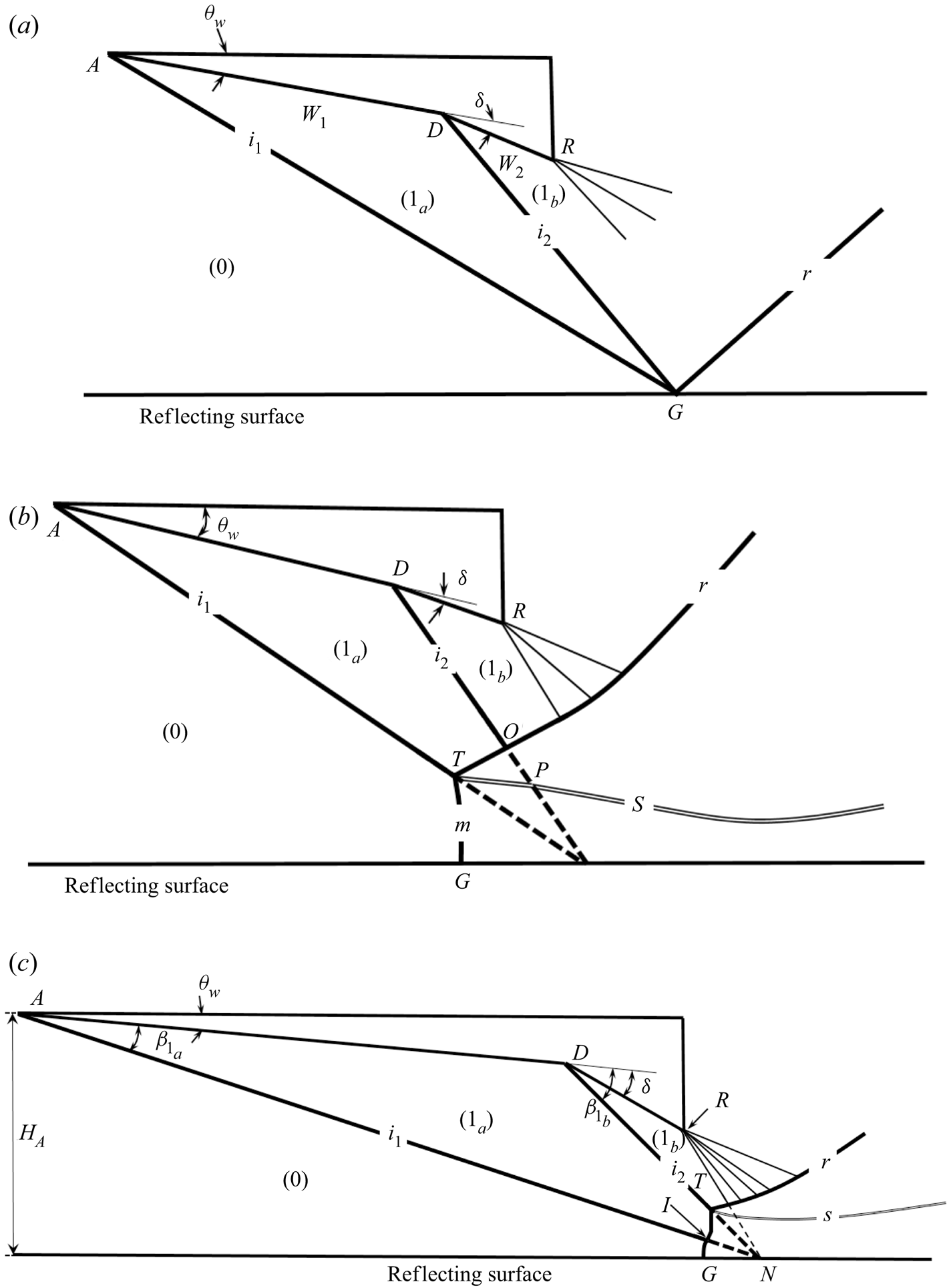
As shown in figure 1, three reflection types may be possible when two incident shock waves reflect at the same point. The first type is regular reflection, as displayed in figure 1(a). The second type, as displayed in figure 1(b), is pre-Mach reflection where it is the first incident shock wave that has Mach reflection. The third type is post-Mach reflection, as depicted in figure 1(c). For post-Mach reflection it is the downstream incident shock wave that has Mach reflection. In the situations displayed in figure 1, the wedge has an initial deflection angle  $\theta _{w}$, which produces the first incident shock wave, and an additional deflection (of angle
 $\delta$) which produces the second incident shock wave. The additional deflection, at point
 $D$, divides the lower wedge surfaces into two segments:
 $AD$ (of width
 $w_{1}$) and
 $DR$ (of width
 $w_{2}$).
Possible shock reflection types with two incident shock waves.  $(a)$ Regular reflection.
 $(b)$ Pre-Mach reflection.
 $(c)$ Post-Mach reflection.

The first two cases have been studied by Guan, Bai & Wu (Reference Guan, Bai and Wu2018), who demonstrated that the second incident shock wave has the role of increasing the height of the Mach stem and advancing the transition to Mach reflection of the first incident shock wave. Guan et al. (Reference Guan, Bai and Wu2020) then concluded that the intersection of the reflected shock wave with the second incident shock wave may produce a double solution. However, the situation of post-Mach reflection, where the second incident shock wave has Mach reflection, has not been considered before and the study of such a situation is the purpose of this paper.
There are three issues that merit study for post-Mach reflection. The first is the critical condition to have post-Mach reflection. The second is the flow configuration in post-Mach reflection. The interference between the first incident shock wave and the Mach stem of the second incident shock wave appears to be extremely interesting, since it normally produces a type IV shock interference and this interference will alter the flow of the duct downstream of the Mach stem. The third is how the Mach stem of the second incident shock wave and the flow downstream of this Mach stem are affected by the first incident shock wave. Clarifying these issues certainly increases our knowledge of shock reflection.
In this paper we will attempt to study these three issues, within the context of inviscid flow of a perfect gas. For this purpose, we will first use shock polar analysis to anticipate the main flow structure. This analysis will be conducted in § 2. The anticipated flow structure will then be confirmed by numerical simulation using computational fluid dynamics. The compressible Euler equations in gas dynamics are solved using a finite volume method based on the second-order Roe scheme (Roe Reference Roe1986). The numerical simulation will be given in § 3, where we also show more details about the flow structures.
The second and third issues will be studied in § 4, where we will derive a necessary condition to have post-Mach reflection and study how Mach reflection of the second incident shock wave is promoted by the upstream incident shock wave. In § 4 we will also discuss, although briefly, how the type IV shock interference between the first incident shock wave and Mach stem affects the Mach stem height and the flow field downstream of the Mach stem. Although the present study is primary for inviscid flow, a numerical result is displayed, in § 4.4, to show that viscosity may have quantitative influence on the Mach stem height and jet width.
In the appendix we will display how the numerical solution depends on the mesh and unsteadiness of solutions.
The problem under study depends only on the geometrical parameters (wedge angles  $\theta _{w}$ and
 $\delta$, the position of the turning point
 $D$) and on the inflow Mach number
 $M_{0}$ and ratio of specific heats
 $\gamma$. For a perfect gas,
 $\gamma$ is constant. When we display quantitative results, we only consider air and set
 $\gamma =1.4$.
In numerical computation we only need to set non-dimensional values for density ( $\rho$), pressure (
 $p$) and temperature (
 $T$) or energy. In this paper we do not consider the real gas effect so that dimensional values are not needed.
The oblique shock wave relations, which can be found in any classical text books of gas dynamics (cf. Ben-Dor, Igra & Elperin Reference Ben-Dor, Igra and Elperin2001), will be repeatedly used in this paper. For brevity, we write the shock wave relations as
 \begin{equation} \tan \theta =f_{\theta }(M_{u},\beta ),\quad M_{d}=f_{M}(M_{u},\beta ),\quad p_{d}=p_{u}\,f_{p}(M_{u},\beta ) \end{equation}
where
 \begin{equation} \left. \begin{aligned}
f_{\theta }({M,\beta }) & =\frac{2\left( {M}^{2}{\sin
}^{2}{\beta }-1\right) }{ ( {M}^{2}\left( \gamma +\cos
{2\beta }\right) +2) \tan {\beta }},\\ f_{M}(M,{\beta
)} & =\sqrt{\frac{\left( \gamma -1\right)
{M}^{2}+2}{2\gamma {M} ^{2}{\sin }^{2}{\beta }-\left(
\gamma -1\right) }+\frac{2{M}^{2}{\cos }^{2}{ \beta
}}{\left( \gamma -1\right) {M}^{2}{\sin }^{2}{\beta
}+2}},\\ f_{p}(M,{\beta )} & =1+\frac{2\gamma }{\gamma
+1}\left( {M}^{2}{\sin }^{2}{ \beta }-1\right).
\end{aligned} \right\}
\end{equation}
Here,  ${\beta }$ is the shock angle,
 $\theta$ is the flow deflection angle across the shock wave, the subscript
 $u$ is for flow parameters upstream of the shock wave and
 $d$ is for flow parameters downstream of the shock wave. Note that, for given
 $M_{u}$ and
 $\theta$, the shock relation gives two values of
 ${\beta }$. The small value
 ${\beta }$ corresponds to weak solution and the large value corresponds to strong solution.
2. Flow structure anticipated by shock polar analysis
2.1. Method of shock polar analysis
The pressure–deflection angle shock polar analysis has been introduced by Kawamura & Saito (Reference Kawamura and Saito1956) for study of shock reflection; see also Ben-Dor (Reference Ben-Dor2007) for more details. Shock polar analysis displays, in the plane  $\theta\hbox{--}p$, the pressure–deflection angle relation
 $p=p(\theta )$ for each shock wave. The relation
 $p=p(\theta )$ is called shock polar and is given by oblique shock wave relation (1.2) for each involved shock wave.
Each polar has a lower part corresponding to weak solutions and an upper part corresponding to strong solutions. Shock waves with different upstream conditions (Mach number and flow deflection angle) follow different polars in the same plane  $\theta\hbox{--}p$. If multiple shock waves may exist in a flow, then the intersection of various shock polars (from various shock waves) defines possible flow pattern created at the interaction point.
A shock polar analysis is helpful in anticipating shock structures produced in complex shock reflection problems (cf. Ben-Dor Reference Ben-Dor2007; Hillier Reference Hillier2007; Yao et al. Reference Yao, Li and Wu2013). For each shock wave with a given upstream Mach number  $M_{u}$, the relations
 $p=p_{u}\,f_{p}(M_{u},\beta )$ and
 $\tan \theta =f_{\theta }({M}_{u}{,\beta })$ are solved to define the shock polar
 $p=p(\theta )$ in the plane
 $\theta\hbox{--}p$.
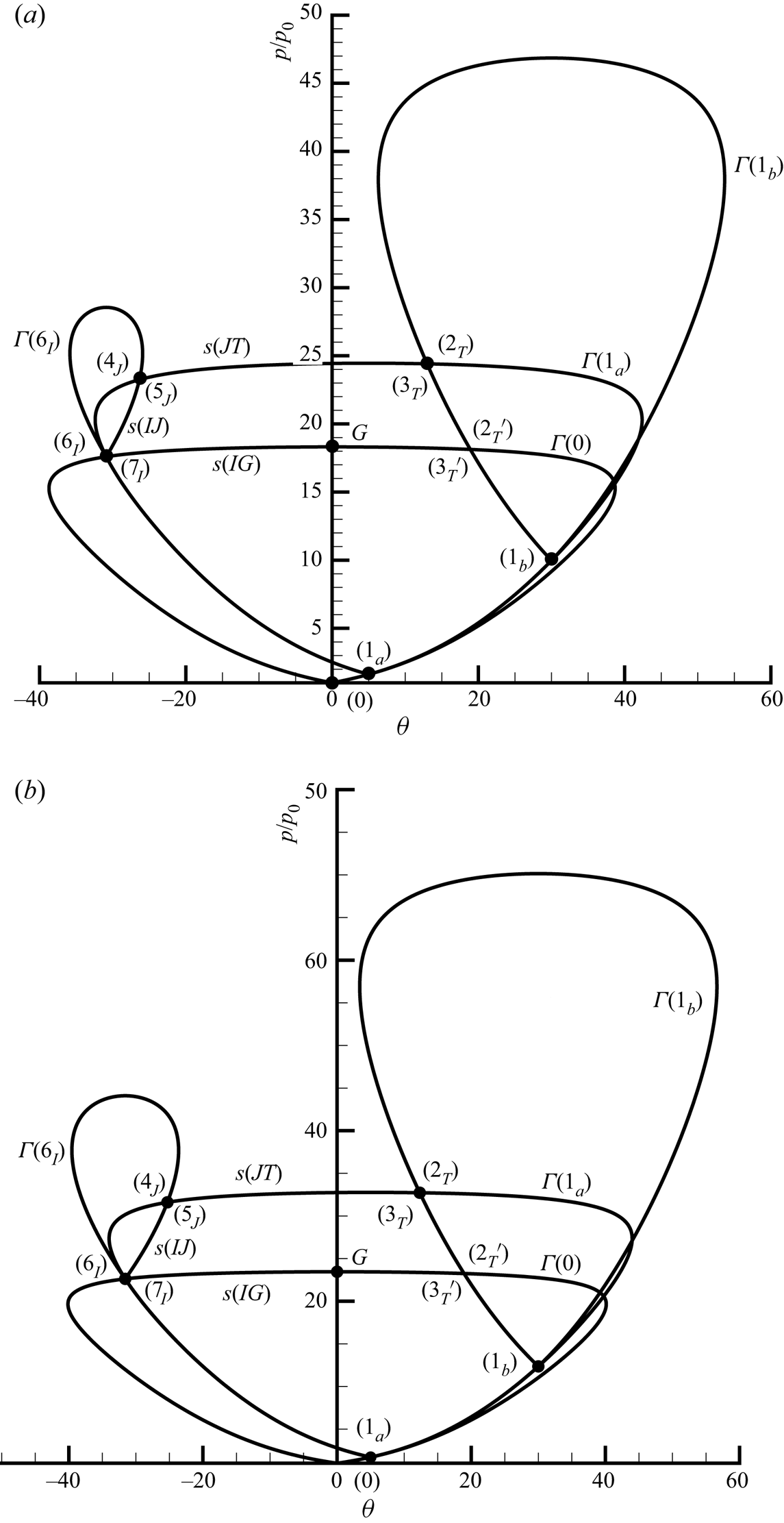
Now the shock polar analysis is applied to the present problem with two incident shock waves. We have considered two cases. In the first case,  $M_{0}=3.98$,
 $\theta _{w}=5^{\circ }$ and
 $\delta =25^{\circ }$. In the second case,
 $M_{0}=4.5$,
 $\theta _{w}=5^{\circ }$ and
 $\delta =25^{\circ }$. For both cases, the downstream shock wave will have Mach reflection according to the transition analysis in § 4.
We use  $\varGamma (k)$ to denote the shock polar, along which is the locus of all the flow states that could be obtained from any shock wave with a fixed upstream state
 $(k)$. The shock polars for the chosen two conditions are displayed in figure 2, where the vertical axis is normalized as
 $p/p_{0}$. The shock polar has similar patterns for both cases, and in fact for other cases in case of post-Mach reflection. Thus, we only provide details of shock polar analysis for the first case.
 $(a)$ Shock polar for
 $M_{0}=3.98$,
 $\theta _{w}=5^{\circ }, \delta =25^{\circ }$.
 $(b)$ Shock polar for
 $M_{0}=4.5$,
 $\theta _{w}=5^{\circ }, \delta =25^{\circ }$.

2.2. Shock polars for the two incident shock waves
The upstream flow is the initial state  $(0)$, at which
 $p/p_{0}=1$ and
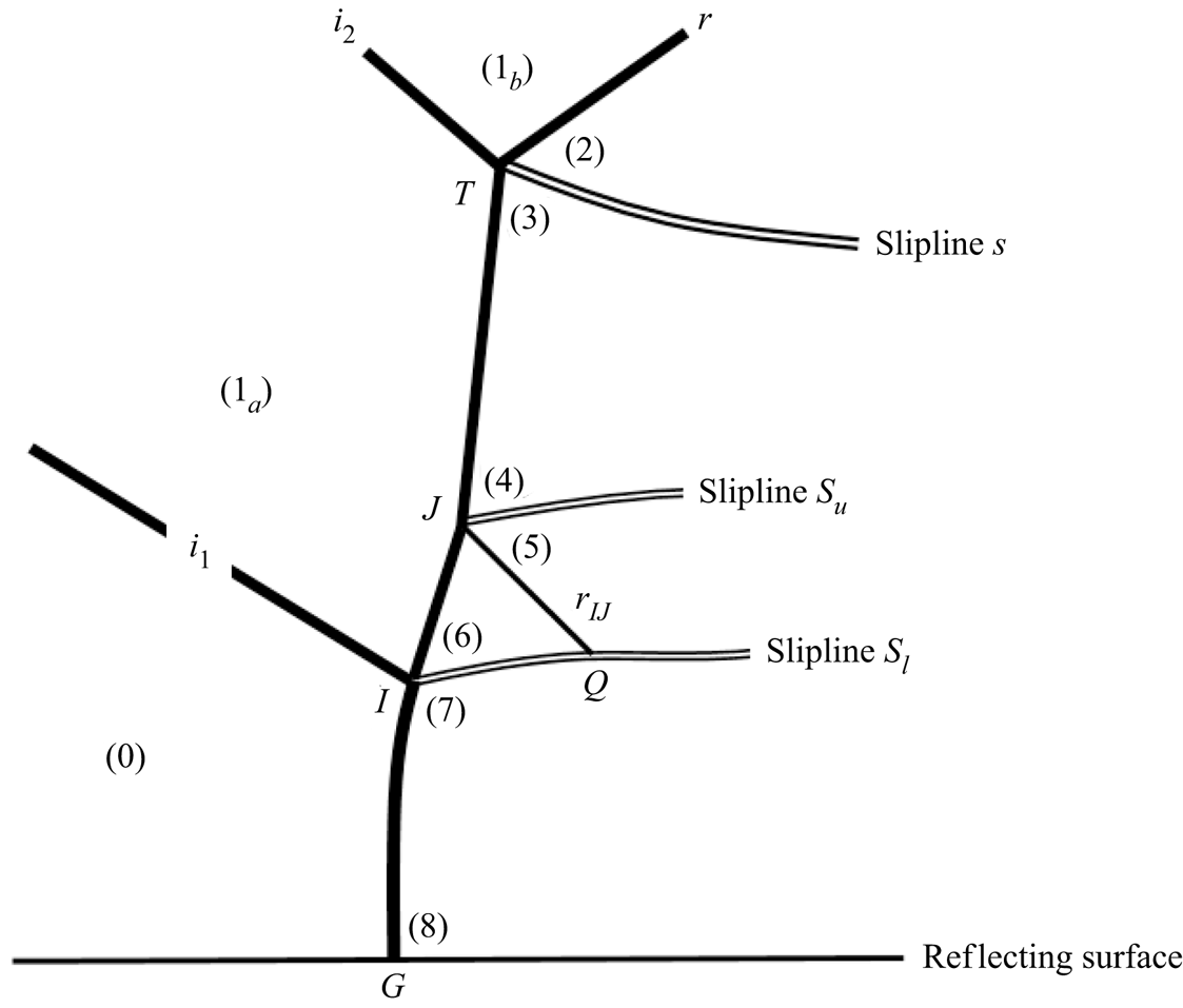
 $\theta _{0}=0$. The shock structures anticipated by shock polar analysis are depicted in figure 3.
An illustration of local Mach reflection configuration for post-Mach reflection.

Polar  $\varGamma (0)$ is the locus of flow states connected to the state (
 $0$) by any shock wave which may be a weak solution such as the first incident shock wave
 $i_{1}$ or a strong solution such as a Mach stem. The state
 $(1_{a})$, connected to the state (
 $0$) by the first incident shock wave
 $i_{1}$, lies at the point
 $(\theta , p/p_{0})=(\theta _{w},p_{1_{a}}/p_{0})$ of polar
 $\varGamma (0)$.
Polar  $\varGamma (1_{a})$ is the locus of flow states connected to the state (
 $1_{a}$) by any shock wave which may be a weak solution such as the second incident shock wave
 $i_{2}$ or a strong solution. The state
 $(1_{b})$, connected to the state (
 $1_{a}$) by the second incident shock wave
 $i_{2}$, lies at the point
 $(\theta , p/p_{0})=(\theta _{w}+\delta ,p_{1_{b}}/p_{0})$ of polar
 $\varGamma (1_{a})$.
2.3. Two triple points identified by shock polar analysis and inverted Mach stem
The shock polars connecting status  $(0)$ and
 $(1_{a})$ have been shown in § 2.2. Here, we continue for other shock polars.
Polar  $\varGamma (1_{b})$ is the locus of flow states connected to the state (
 $1_{b}$) by any shock wave and has an intersection at point
 $T$ with the polar
 $\varGamma (1_{a})$. This intersection yields two flow states, one is
 $(2_{T})$ downstream of the reflected shock wave (denoted by
 $r$ in figure 3) and the other is
 $(3_{T})$ downstream of the Mach stem. Point
 $T$ is the triple point connecting the second incident shock wave, the reflected shock wave and the Mach stem. The flow states
 $(2_{T})$ and
 $(3_{T})$ in figure 2 correspond to the flow states
 $(2)$ and
 $(3)$ in figure 3, which are infinitely close to the triple point
 $T$.
Now we show the intersection point  $I$ is in fact another triple point. We see from figure 2 that the upper-left part of polar
 $\varGamma (0)$ has an intersection with the lower-left part of polar
 $\varGamma (1_{a})$. The upper-left part of polar
 $\varGamma (0)$ is due to a strong shock wave, the state behind it is denoted
 $(7_{I})$, which is flow region
 $(7)$ infinitely close to point
 $I$ as shown in figure 3. This strong shock wave can be viewed as the Mach stem produced by reflection of the first incident shock wave.
However, the condition we choose is below the von Neumann condition for the first incident shock wave. If Mach reflection exists it must be an inverse Mach reflection according to Hekiri & Emanuel (Reference Hekiri and Emanuel2015). The intersection of this inverted Mach stem with the first incident shock wave defines another triple point and this triple point is just the intersection point  $I$ as shown in figure 3. The reflected shock wave pertinent to this triple point (
 $I$) will be denoted by
 $s(IJ)$. Here, as shown below,
 $J$ will be another triple point lying between the triple points
 $I$ and
 $T$.
Downstream of  $s(IJ)$ is the state
 $(6_{I})$ which also lies on the lower-left part of polar
 $\varGamma (1_{a})$ and which corresponds to flow region
 $(6)$ in figure 3. It is verified that shock
 $s(IJ)$ is a weak shock wave.
2.4. Identification of a third triple point
The two triple points  $T$ and
 $I$ both lie on the entire Mach stem (shock
 $TG$ as shown in figure 3). The states
 $(6_{I})$ and
 $(3_{T})$ are both behind the shock segment
 $IT$, with the state
 $(6_{I})$ close to
 $I$ and
 $(3_{T})$ close to
 $T$. Close to point
 $T$ the segment
 $IT$ is a strong solution, and close to point
 $I$ this segment is a weak one as pointed above.
Now we draw shock polar  $\varGamma (6_{I})$ which connects any state to the state
 $(6_{I})$ by any shock wave. The shock polar
 $\varGamma (6_{I})$ has an intersection with the upper-left part of shock polar
 $\varGamma (1_{a})$, producing two new states, denoted by
 $(4_{J})$ and
 $(5_{J})$. The state
 $(4_{J})$ is a strong shock wave solution and is behind the Mach stem segment
 $TJ$. State
 $(5_{J})$ is behind a shock wave (denoted
 $r_{IJ}$) downstream of the shock wave
 $s(IJ)$ shown in figure 3.
The shock wave  $s(IJ)$, the Mach stem
 $JT$ and the shock
 $r_{IJ}$ are connected to the point
 $J$ which may be regarded as the third triple point. For this triple point,
 $s(IJ)$ may be regarded as the incident shock wave,
 $r_{IJ}$ is the reflected shock wave, and
 $JT$ is the Mach stem, as if a reflecting surface were above the triple point
 $J$.
2.5. Type IV shock interference
The shock polar analysis shows that, apart from the Mach reflection configuration associated with the usual triple point ( $T$), the intersection of the first incident shock wave with the Mach stem leads to a flow configuration that can not only be regarded as a type IV shock interaction pattern but also as an inverted Mach reflection configuration.
It is well known that the intersection of an incident shock wave with a bow shock leads to six types of shock interference (Edney Reference Edney1968). According to Keyes & Hains (Reference Keyes and Hains1973), when a weak impinging shock intersects the nearly normal part of a strong shock wave, a type IV interference occurs. This interference results in a complex flow pattern which will further spoil the Mach reflection structure. Many studies have been conducted for type IV interference (cf. Grasso, Purpura & Chanetz Reference Grasso, Purpura, Chanetz and Delery2003).
Here, it is the first incident shock wave that intersects the Mach stem. Since the Mach stem is a strong shock wave which is nearly normal (Li & Ben-Dor Reference Li and Ben-Dor1997), a type IV shock interference occurs.
3. Numerical study of the flow structure
3.1. Geometry condition and numerical method
The geometry of the configuration depends on the flow condition if the two incident shock waves intersect at the same point on the reflecting surface (Guan et al. Reference Guan, Bai and Wu2018). To give the geometrical parameters we choose a coordinate system  $(x,y)$ such that
 $x_{A}=0$ and
 $y_{A}=0$. Here
 $A$ is the leading edge of wedge, see figure 1(c). Since we are considering the problem that the two incident shock waves reflect at the same point, the position of reflection point
 $(x_{N}$,
 $y_{N})$ can be shown to satisfy
 \begin{equation} \left. \begin{aligned} x_{N} & =\frac{\tan \left( \beta _{1_{b}}+\theta _{w}\right) \cos \theta _{w}-\sin \theta _{w}}{\tan \left( \beta _{1_{b}}+\theta _{w}\right) -\tan \beta _{1_{a}}}w_{1},\\ y_{N} & =-\frac{\tan \left( \beta _{1_{b}}+\theta _{w}\right) \cos \theta _{w}-\sin \theta _{w}}{\tan \left( \beta _{1_{b}}+\theta _{w}\right) -\tan \beta _{1_{a}}}w_{1}\tan \beta _{1_{a}}, \end{aligned} \right\} \end{equation}
once  $M_{0},\theta _{w},\delta$ and
 $w_{1}$ are given.
We do not consider the case that the leading characteristic of the expansion fan intersects the second incident shock wave in the case of regular reflection. In numerical simulation we simply consider the situation that the leading characteristics intersect the reflection point  $N$ shown in figure 1(c). Under this requirement, the use of (3.1) leads to the following relation
 \begin{equation} w_{2}=\frac{y_{N}+w_{1}\left[ \sin \theta _{w}-\cos \theta _{w}\tan \left( \theta _{w}+\delta +\mu _{1_{b}}\right) \right] +x_{N}\tan \left( \theta _{w}+\delta +\mu _{1_{b}}\right) }{\cos \left( \theta _{w}+\delta \right) \tan \left( \theta _{w}+\delta +\mu _{1_{b}}\right) -\sin \left( \theta _{w}+\delta \right) } \end{equation}
to determine  $w_{2}$; see figure 1(a) for the definition of
 $w_{2}$. Here,
 $\mu _{1_{b}}=\arcsin ({1}/{M_{1_{b}}})$ is the Mach angle. The expressions to determine
 $\beta _{1_{a}}$,
 $\beta _{1_{b}}$ and
 $M_{1_{b}}$ follow from the oblique shock wave relations.
For numerical simulation the compressible Euler equations in gas dynamics are solved using finite volume method based on the second-order Roe scheme (Roe Reference Roe1986), in the same way as Lin, Bai & Wu (Reference Lin, Bai and Wu2019). This numerical method exists in the commercial code Fluent and has been used by Lin et al. (Reference Lin, Bai and Wu2019) for asymmetrical shock reflection study, which authors validated the suitability of this numerical method in asymmetrical shock reflection against two experimental results of asymmetrical reflection given by Sudani et al. (Reference Sudani, Sato, Karasawa, Noda, Tate and Watanabe2002) and Li, Chpoun & Ben-Dor (Reference Li, Chpoun and Ben-Dor1999), respectively.
3.2. Observation of inverted Mach stem and jet
Two sets of conditions have been used in shock polar analysis. Here, we use these two sets of conditions for numerical simulation.
Recall that the first set has  $M_{0}=3.98$,
 $w_{1}=1.1$,
 $\theta _{w}=5^{\circ }$ and
 $\delta =25^{\circ }$. For this case, the upstream incident shock wave alone only allows for regular reflection and according to the criterion derived in the next section, the downstream incident shock wave has Mach reflection. There is some flexibility to choose
 $w_{2}$. Here, we use (3.1) to get
 $y_{N}=-0.485$ and
 $H_{A}=-y_{N}=0.485$. The length
 $w_{2}$ is then computed by (3.2) and we get
 $w_{2}=0.276$.
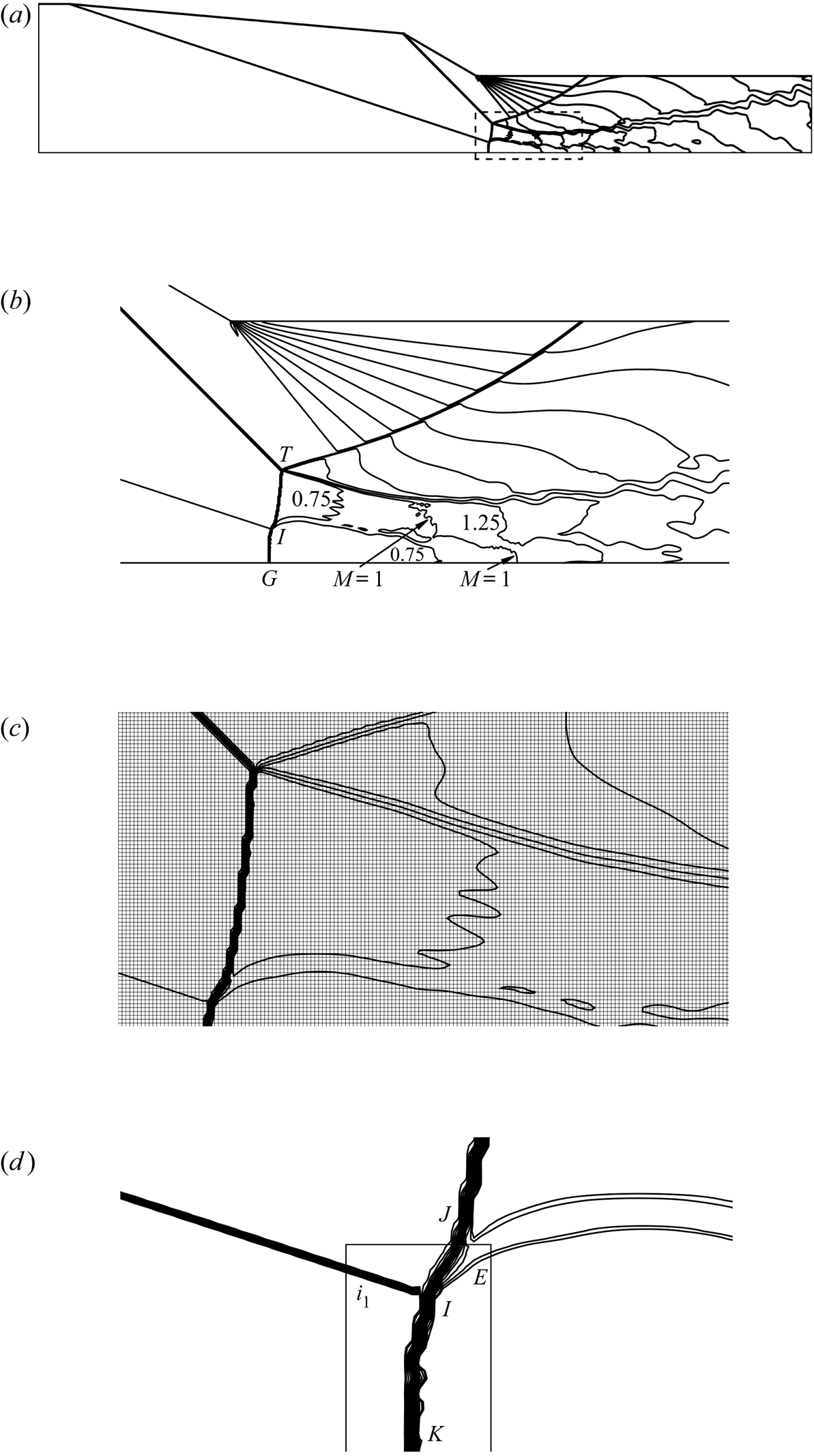
The Mach number contours for a uniform grid with  $2600\times 500$ cells are displayed in figure 4(a–d). Figure 4(a) is a global view from which the main flow structures can be clearly seen.
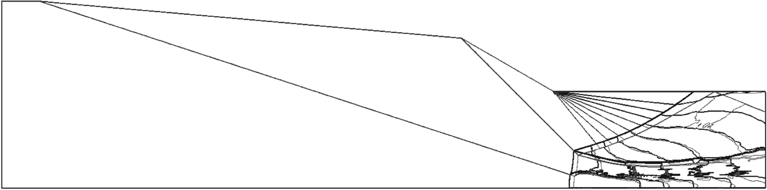
Mach number contours for  $M_{0}=3.98$,
 $\theta _{w}=5^{\circ }$ and
 $\delta =25^{\circ }$, showing post-Mach reflection.
 $(a)$ The overall flow,
 $(b)$ the enlarged view into the frame,
 $(c)$ the mesh into the frame,
 $(d)$ an inverse Mach reflection inside the box.

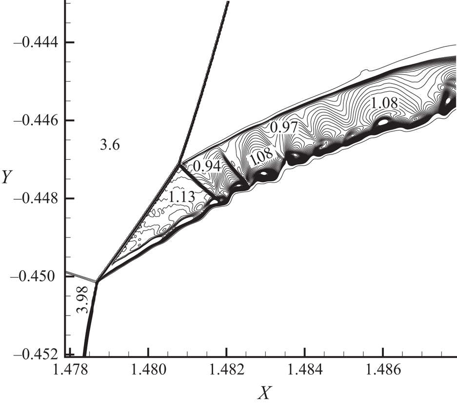
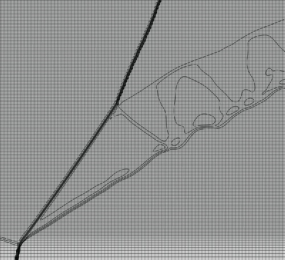
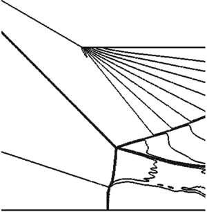
Figure 4(b) shows that the flow duct behind the Mach stem is divided by a jet into two flow ducts. Figure 4(c) gives the mesh near the jet. Figure 4(d) displays the details near the interaction point ( $I$), where we see clearly a jet and an inverted Mach stem as anticipated theoretically in the previous section.
This finding offers another occasion to have inverted Mach reflection, knowing that a downstream pressure perturbation or a second incident shock wave may reverse the Mach stem to an inverted one (Ben-Dor et al. Reference Ben-Dor, Elperin, Li and Vasiliev1999; Guan et al. Reference Guan, Bai and Wu2018) and a blunt body placed along the reflecting surface and downstream of the Mach stem also pushes the Mach stem to be convex toward the upstream direction (Roye, Henderson & Menikoff Reference Roye, Henderson and Menikoff1998).
A grid refinement study is provided in the appendix. Figure 5 shows the Mach number contours displaying the detailed flow structure inside the initial part of the jet (where the grid is refined), obtained from grid C (see the appendix). The number of contours is chosen such that the detailed flow structure inside the jet is clearly visible. It appears that, apart from an initial supersonic portion, the jet is transonic.
Local view of Mach number contours for  $M_{0}=3.98$,
 $w_{1}=1.1,$
 $\theta _{w}=5^{\circ }$ and
 $\delta =25^{\circ }$ using a grid with
 $5000\times 1000$ cells in total.

Note that, for type IV shock interference, the jet is generally unsteady (Gaitonde & Shang Reference Gaitonde and Shang1995; Khatt & Jagadeesh Reference Khatt and Jagadeesh2018) so that when the grid is refined near the jet, the computation cannot converge to a steady state. For the present problem, the influence of unsteadiness of the flow structure and Mach stem height is briefly studied in the appendix.
Consider now the second set of conditions, which has  $M_{0}=4.5,$
 $\theta _{w}=5^{\circ }$ and
 $\delta =25^{\circ }$. For this computation we also set
 $w_{1}=1.1$. By (3.1),
 $y_{N}=-0.425$ so we set
 $H_{A}=-y_{N}=0.425$. The length
 $w_{2}$ is computed by (3.2) and we get
 $w_{2}=0.248$. The grid has approximately
 $4400\times 1400$ cells in total and
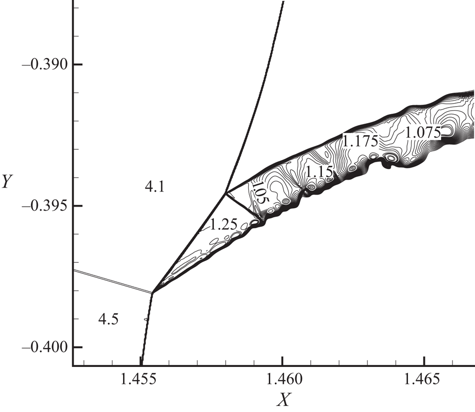
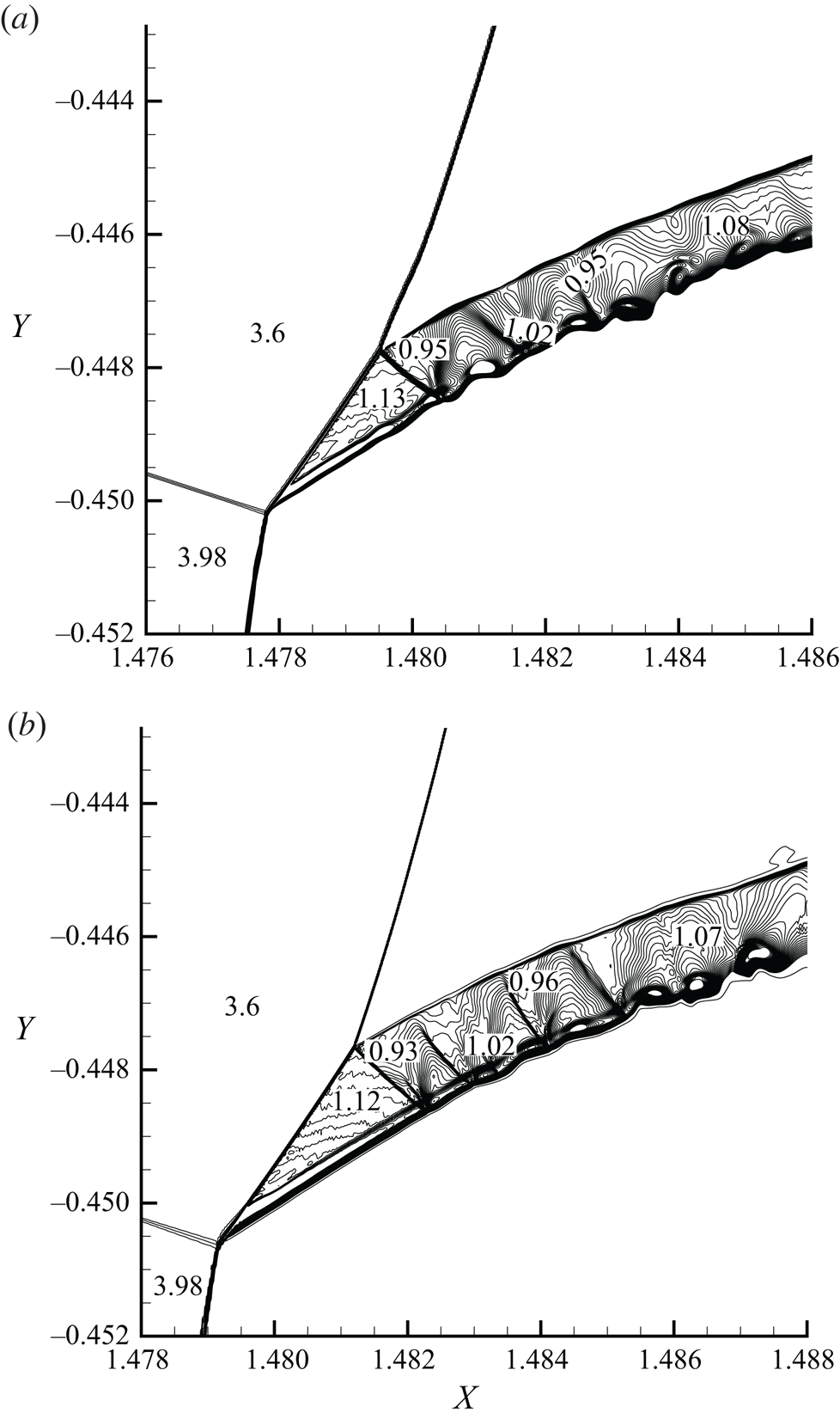
 $2520\times 1120$ cells in the refined region. The local view of Mach number contours displaying details in the jet region is shown in figure 6. In this case we observe a pure supersonic jet, with multiple oblique shock waves and expansion fans zigzagging inside the jet.
Mach number contours for  $M_{0}=4.5$,
 $\theta _{w}=5^{\circ }$ and
 $\delta =25^{\circ }$, displaying a pure supersonic jet.

Type IV shock interference is known to produce a supersonic jet (Keyes & Hains Reference Keyes and Hains1973; Grasso et al. Reference Grasso, Purpura, Chanetz and Delery2003). The present study seems to suggest the jet may be transonic in some conditions. This observation will be studied in the future for the broader problem of type IV shock interference.
4. Influence of the upstream shock wave
4.1. Promotion of Mach reflection by the upstream shock wave
Here, we only consider the detachment criterion for the downstream incident shock wave to have Mach reflection and we will study how this condition is affected by the upstream incident shock wave.
For a given inflow condition with Mach number  $M_{0}$ and pressure
 $p_{0}$, the flow parameters downstream of the upstream shock wave (
 $i_{1}$) are given by
 $M_{1_{a}}=f_{M}(M_{0},\beta _{1_{a}}),$
 $p_{1a}=p_{0}\,f_{p}(M_{0},\beta _{1_{a}})$, where
 ${\beta }_{1_{a}}$ is solved from
 $\tan \theta _{w}=f_{\theta }(M_{0},\beta _{1_{a}})$ for a weak shock wave.
The flow parameters downstream of the downstream incident shock wave ( $i_{2}$) are then given by
 $M_{1_{b}}=f_{M}(M_{1_{a}},\beta _{1_{b}}),$
 $p_{1b}=p_{1_{a}}\,f_{p}(M_{1_{a}},\beta _{1_{b}})$ where
 ${\beta }_{1_{b}}$ is solved from
 $\tan \delta =f_{\theta }(M_{1_{a}},\beta _{1_{b}})$ also for a weak shock wave.
The detachment condition for Mach reflection of the downstream shock wave corresponds to a turning angle  $\delta$ with which the total flow deflection angle
 $\theta _{w}+\delta$ of the reflected shock wave (
 $r$) downstream of
 $(i_{2})$ is exactly equal to the usual detachment angle determined by the upstream Mach number
 $M_{1_{b}}$.
For each choice of  $M_{0}$ and
 $\theta _{w}$, this detachment condition determines a
 $\delta =\delta ^{(D)}(M_{0},\theta _{w})$ and Mach reflection of the downstream shock wave occurs when
 $\delta >\delta ^{(D)}(M_{0},\theta _{w})$.
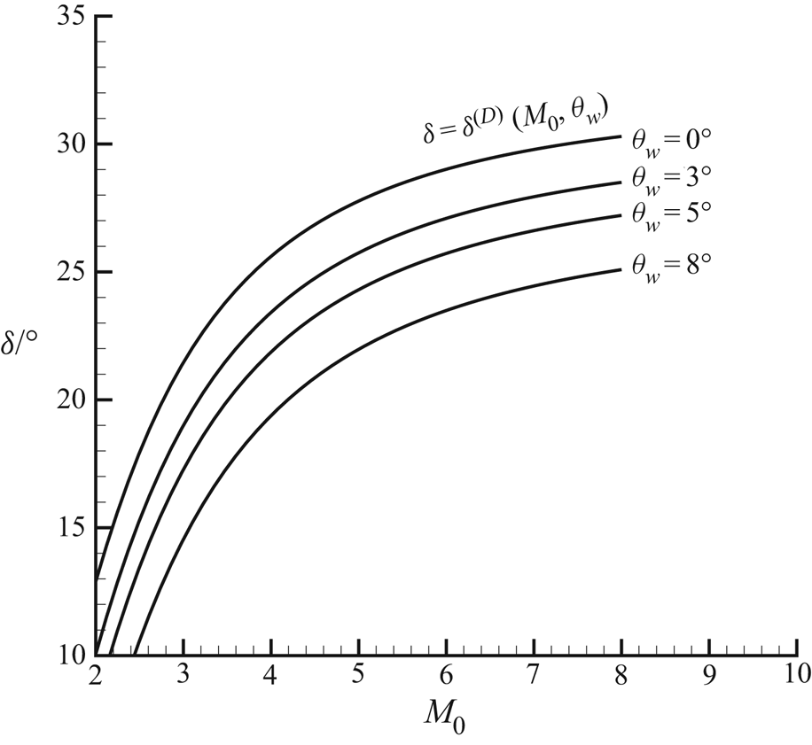
Figure 7 displays the condition  $\delta =\delta ^{(D)}(M_{0},\theta _{w})$ in the
 $M_{0}\hbox{--}\delta$ plane, for
 $\theta _{w}=0^{\circ },3^{\circ },5^{\circ },8^{\circ }$. The choice of various values of
 $\theta _{w}$ is for purpose of showing how the transition to Mach reflection of the downstream shock wave is affected by the strength of the upstream shock wave. It is verified that we produce the same results as Mouton (Reference Mouton2007) when
 $\theta _{w}=0$ (which is the single incident shock wave case). It is clear that
 $\delta ^{(D)}(M_{0},\theta _{w})$ is lowered by increasing
 $\theta _{w}$, meaning that Mach reflection of a shock wave is promoted by the existence of an upstream incident shock wave.
Detachment conditions in the plane  $( M_{0}, \delta )$ for
 $M_{0}=3.98$ and
 $\theta _{w}=0^{\circ },3^{\circ },5^{\circ },8^{\circ }.$

4.2. Heights of Mach stem and jet
To understand how the Mach stem height is affected by inflow Mach number and geometry, we first recall how the Mach stem height varies according to the wedge angle and the inflow Mach number for shock reflection of a single incident shock wave.
According to previous studies for Mach stem height of a single incident shock wave (Hornung & Robinson Reference Hornung and Robinson1982; Li & Ben-Dor Reference Li and Ben-Dor1997; Mouton & Hornung Reference Mouton and Hornung2007; Gao & Wu Reference Gao and Wu2010), the Mach stem height is an increasing function of wedge angle for fixed inflow Mach number, see for instance figure 14(c,d) of Gao & Wu (Reference Gao and Wu2010), and a decreasing function of the inflow Mach number for fixed wedge angle, see for instance figure 14(a,b) of Gao & Wu (Reference Gao and Wu2010).
Now we consider Mach reflection subjected to influence of an upstream shock wave, with the conditions  $w_{1}=1.1,$
 $\theta _{w}=5^{\circ }$. We check whether the Mach stem height is also a decreasing function of
 $M_{0}$, for a fixed
 $\delta$.
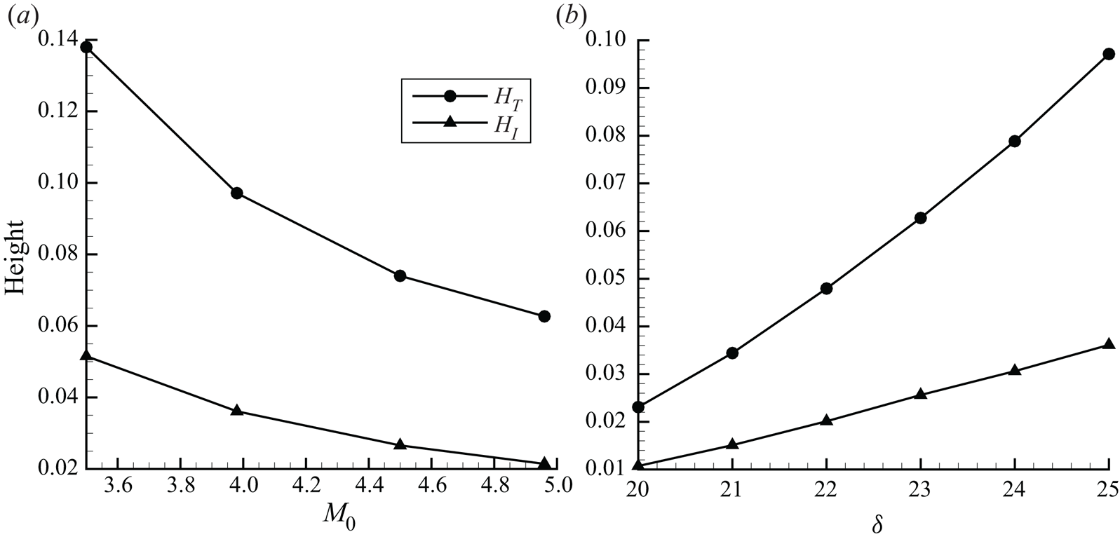
For  $\delta =25^{\circ }$, the influence of
 $M_{0}$ on
 $H_{T}$ and
 $H_{I}$ is displayed in figure 8(a). It is seen that both
 $H_{T}$ and
 $H_{I}$ are decreasing functions of
 $M_{0}$. Since in this case the condition for upstream incident shock wave is fixed, the decrease of
 $H_{T}$ for increasing
 $M_{0}$ is similar to the decrease of Mach stem for increasing Mach number of Mach reflection of a single incident shock wave.
The influence of the jet on the Mach stem height and the position of the interference point.  $(a)$ For
 $w_{1}=1.1,$
 $\theta _{w}=5^{\circ }$,
 $\delta =25^{\circ },M_{0}$ varies.
 $(b)$ For
 $M_{0}=3.98$,
 $w_{1}=1.1,$
 $\theta _{w}=5^{\circ }$,
 $\delta$ varies.

For fixed  $\delta$ and
 $M_{0}$, it can be easily argued that the Mach stem height
 $H_{T}$ and jet height
 $H_{I}$ are increasing functions of
 $\theta _{w}$, since increasing
 $\theta _{w}$ will decrease the upstream Mach number
 $M_{1_{a}}$ of the downstream shock wave and according to the above knowledge of single incident shock wave reflection this increases the Mach stem height.
The influence of  $\delta$ on
 $H_{T}$ and
 $H_{I}$ for a fixed inflow Mach number appears to be not so evident. For
 $M_{0}=3.98$, the influence of
 $\delta$ on
 $H_{T}$ and
 $H_{I}$ is displayed in figure 8(b). It is seen that both
 $H_{T}$ and
 $H_{I}$ are increasing functions of
 $\delta$. Since in this case the condition for upstream incident shock wave is fixed, the increase of
 $H_{T}$ for increasing
 $\delta$ is similar to the increase of Mach stem for increasing wedge angle of Mach reflection of a single incident shock wave.
According to the mesh convergence and time history study provided in the appendix, the uncertainty of Mach stem height is approximately  $1.02\,\%$ due to mesh resolution and
 $1.65\,\%$ due to time oscillation. This uncertainty is small enough so that the above conclusion will not be changed by numerical error or time oscillation.
4.3. Complexity of the mechanism determining the Mach stem height
The mechanism by which the size of a Mach reflection is determined, a question raised by Courant & Friedrichs (Reference Courant and Friedrichs1948), is complex even for Mach reflection of a single incident shock wave. Li & Ben-Dor (Reference Li and Ben-Dor1997) pointed out that the expansion fan due to the wedge determines the size and location of the Mach stem by creating the sonic throat and carrying information on the upper geometrical conditions through the subsonic pocket to the Mach stem. Bai & Wu (Reference Bai and Wu2017) proposed a sonic throat compatibility condition to determine the size of the Mach stem.
For the present case, the jet divides the flow downstream of the Mach stem into two flow ducts. The upper duct is between the slipline from triple point ( $T$) and the upper boundary of the jet. The lower duct is between the lower boundary of the jet and the reflecting surface. As can be seen from figure 4(b), the upper duct and lower duct each have a sonic throat of different location.
The existence of sonic throat for the upper duct is due to the pressure-decreasing expansion waves from the wedge corner. The upper duct initially converges, the pressure-decreasing expansion waves make it finally diverge so that a sonic throat exists.
The lower duct is initially divergent, due to inverse Mach reflection. Then, the lower duct is subjected to the effect of the pressure decreasing gradient coming from the upper duct so that it finally converges and then diverges.
Since the lower duct initially diverges, it needs a longer distance with pressure-decreasing effect to create the sonic throat. Moreover, there is some time lagging in the transmission of pressure-decreasing waves across the transonic jet. Hence, the sonic throat in the lower duct appears far downstream of that in the upper duct.
The difference of sonic throat positions in the two flow ducts makes it very difficult to build a theoretical model to predict the Mach stem heights.
4.4. Viscous effect
The influence of viscosity on shock reflection has been studied for single incident shock wave reflection. Schmisseur & Gaitonde (Reference Schmisseur and Gaitonde2011) used numerical simulations to show that viscosity has two effects. The viscosity increases the Mach stem height due to the increased displacement effect of the wedge boundary layer on Mach reflection. Chen, Bai & Wu (Reference Chen, Bai and Wu2020) derived a simple model to account the displacement effect of the boundary layer. The viscosity also thickens the shear layer emanating from the triple point and this thickening may also have some influence since the pressure across the shear layer balances over a finite distance. Schmisseur & Gaitonde (Reference Schmisseur and Gaitonde2011) also showed that no significant differences between inviscid and viscous calculations exist in the shear layers emanating from the triple point.
However, the present problem contains a narrow jet that may be sensitive to viscosity. A detailed study is beyond the scope of this study. Here, we only display one result, for  $M_{0}=3.98$,
 $w_{1}=1.1$,
 $\theta _{w}=5^{\circ }$ and
 $\delta =25^{\circ }$. The Reynolds number based on the inlet height is
 $10^{7}$. The numerical result is obtained by solving the Navier–Stokes equations. The inviscid part is solved using the same method as for inviscid flow and the viscous part is solved using second-order central differences. For turbulence, the Reynolds-averaged Navier–Stokes (RANS)
 $k\hbox{--}\omega$ shear stress transfer (SST) model is used. In the inlet we provide the turbulent kinetic energy
 $k=0.8$ and specific dissipation rate
 $\omega =0.8$.
The grid we use is similar to grid C (of the appendix), but with additional refinement near the lower surface of the wedge to resolve the boundary layer. The global Mach number contours for the comparison of inviscid and viscous flow are displayed in figure 9, by steady state computation using  $1.02\times 10^{6}$ time iterations. Here, the black lines are for inviscid flow and the grey lines are for viscous flow. Hence, compared to inviscid flow solution, the Mach stem is pushed towards the downstream direction by viscosity.
Comparison of Mach contours of viscous (grey lines) and inviscid (black lines) computations, with  $M_{0}=3.98$,
 $w_{1}=1.1$,
 $\theta _{w}=5^{\circ }$ and
 $\delta =25^{\circ }$. For viscous flow the Reynolds number is
 $10^{7}$.

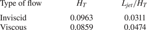
As shown in table 1, viscosity decreases the Mach stem height but increases the jet width  $L_{jet}$, by nearly
 $20\,\%$ for the flow conditions considered. This result suggests that in real applications (with specific choice of Reynolds number), one cannot just use inviscid simulation if quantitative information is required. Normally, the boundary layer will increase the effective wedge angle so that the Mach stem height should increase (Schmisseur & Gaitonde Reference Schmisseur and Gaitonde2011; Chen et al. Reference Chen, Bai and Wu2020). Here, the decrease of the Mach stem height due to viscosity would be associated with the increase of the thickness of the jet. The exact mechanism is difficult to explain, for a similar reason to that discussed in § 4.3 for inviscid flow.
Sizes of Mach stem segment and jet for inviscid and viscous flows, with  $M_{0}=3.98$,
 $w_{1}=1.1$,
 $\theta _{w}=5^{\circ }$ and
 $\delta =25^{\circ }$. For viscous flow the Reynolds number is
 $10^{7}$.

5. Conclusion
Mach reflection by two incident shock waves has been recently studied by Guan et al. (Reference Guan, Bai and Wu2018). Guan et al. (Reference Guan, Bai and Wu2018) considered the case of pre-Mach reflection, where it is the first incident shock wave that has a Mach reflection and the Mach stem is subjected to the influence of the downstream one.
Here, in this paper, we have considered post-Mach reflection for shock reflection by two incident shock waves, where it is the downstream incident shock wave that has Mach reflection and this Mach reflection is subjected to the influence of the upstream incident shock wave.
We have used shock polar analysis to identify the flow structure and derived a detachment condition to have post-Mach reflection. We also have used computational fluid dynamics to verify the theoretical prediction and to study the detailed flow structure.
By shock polar analysis, we have shown that post-Mach reflection produces an inverted Mach stem and type IV shock interference between the Mach stem and the upstream shock wave. This shock interference produces a jet that divides the flow stream downstream of the Mach stem into two ducts with different sonic throats, thus complicating the mechanism by which the Mach stem size is determined. A transition analysis shows that the Mach reflection of the downstream shock wave is promoted by the upstream one. Computational fluid dynamics demonstrates how the heights of Mach stem and jet depend on the inflow Mach number and wedge turning angle.
Type IV shock interaction was believed to yield a supersonic jet downstream of the interaction point. However, we observed here a transonic jet for a specific choice of flow condition. This issue will be studied in the future for the broader problem of type IV shock interference.
The unsteadiness associated with the jet and the influence of viscosity also deserve further study. A viscous simulation shows that viscosity may have an important influence on the Mach stem height and jet width.
Acknowledgements
The authors are grateful to all referees for their valuable comments that helped to improve the manuscript. This work was supported partly by the National Key Project (Grant No. GJXM92579) and by the National Science and Technology Major Project 2017-II-003-0015. Part of the work of C.Y.B. has been conducted in Tsinghua University.
Declaration of interests
The authors report no conflict of interest.
Appendix. Numerical solution under mesh refinement and time iteration
The uniform grid with  $2600\times 500$ cells used in § 3.2 correctly captured post-Mach reflection, inverted Mach stem and jet, as anticipated by theoretical analysis in § 2, while the flow structures inside the jet is not clearly resolved using such a grid.
Now we refine the grid in the jet to display more details in order to show the nature of the jet. However, the jet is narrow and long, so refining the grid everywhere in the jet requires a huge number of grid points. Here, we just refine the region enclosing the initial part of the jet. This refined leading part has a length approximately 10 times the width of the jet. The refined grid is still a structured one.
The problem is, however, further complicated by the unsteadiness of numerical solution even after hundreds of thousands of time iterations. Hence, we not only need to examine mesh convergence but also time convergence of the flow structure inside the jet. The purpose is to demonstrate the topography of the flow structure inside the jet should no longer change after further mesh refinement and further time iterations. Five refined grids are considered.
(i) Grid A has in total
 $3600\times 730$ cells with the refined region containing $1400\times 280$ cells.
(ii) Grid B has in total
$4300\times 970$ cells with the refined region containing $2100\times 420$ cells.(iii) Grid C has in total
$5000\times 1000$ cells with the refined region containing $2800\times 560$ cells. The local refined mesh for grid C, as compared to figure 4(c), is displayed in figure 10.(iv) Grid D has
$6450\times 1390$ cells with the refined region containing $4200\times 840$ cells.(v) Grid E has
$7500\times 1500$ cells with the refined region containing $5600\times 1120$ cells.


Refined mesh grid (grid C) near the jet for  $M_{0}=3.98$,
 $w_{1}=1.1$,
 $\theta _{w}=5^{\circ }$ and
 $\delta =25^{\circ }$.

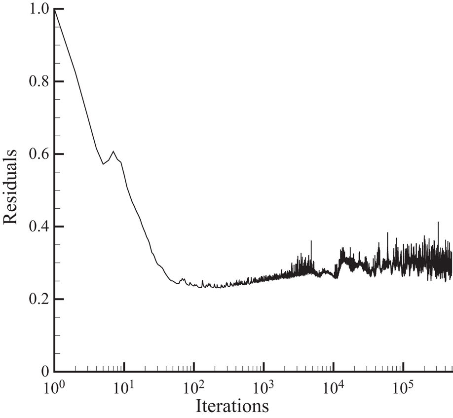
In fact, both steady and unsteady approaches should converge to a steady state solution if the problem indeed has a steady solution. If the problem has an unsteady solution, as in the present case with a jet, an approach with a very coarse grid and with a highly dissipative numerical scheme would lead to a steady solution. Since we used a highly dense mesh to resolve the flow structure, we have obtained unsteadiness with both steady and unsteady approaches. The time history of the density residuals, defined as the root mean square of density variations between two subsequent time iterations, is displayed in figure 11 for grid D. Here, the computation is done using a Courant number  $0.5$.
The residual curve of density for  $M_{0}=3.98$,
 $\theta _{w}=5^{\circ }$ and
 $\delta =25^{\circ }$, computed using grid D.

Below we summarize the results.
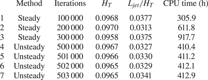
(a) The computation does not converge in time but the topography of the jet does not change in time. As shown in figure 12(a), the jet at time iteration  $5\times 10^{5}$ has the same topography as that at time iteration
 $1\times 10^{5}$ displayed in figure 5, in the sense that the jets predicted at both time iterations. Table 2 shows, for grid C, the Mach stem height
 $H_{T}$ and relative jet length
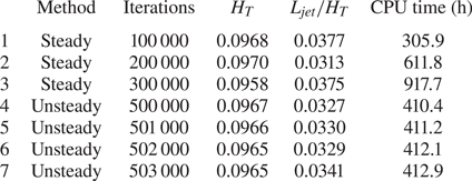
 $L_{jet}/H_{T}$ at three different time iterations for both steady and unsteady computations. We see both the Mach stem height and the relative jet length change a little in time. Table 2 also gives the CPU times.
Local view of Mach number contours for  $M_{0}=3.98$,
 $w_{1}=1.1,$
 $\theta _{w}=5^{\circ }$ and
 $\delta =25^{\circ }$.
 $(a)$ Grid C after
 $5\times 10^{5}$ time iterations.
 $(b)$ Grid E after
 $1\times 10^{5}$ time iterations the same as that used with grid C in § 3.2.

Mach stem height ( $H_{T}$) and relative width
 $(L_{jet}/H_{T}$) of the initial part of the jet for different grids at different numbers of iterations, for
 $M_{0}=3.98$,
 $w_{1}=1.1$,
 $\theta _{w}=5^{\circ }$ and
 $\delta =25^{\circ }$. The computation is run on a multi-core supercomputer, with 48 cores used for steady case and 240 cores for the unsteady case.
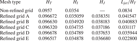
(b) The computation does not converge in space but the topography of the jet does not change with different grids. Table 3 displays the heights  $H_{T},H_{I}$ and
 $H_{J}$ of the three triple points
 $T,I$ and
 $J$ and the relative initial width
 $L_{jet}/H_{T}$ of the jet. Although the three heights do not change much with different refined grids, the relative initial width
 $L_{jet}/H_{T}$ of the jet changes a lot when different grids are used. This means that the result is not mesh converged. However, the topography of the flow structure inside the jet remains the same for different grids, as can be seen from figure 12(b), which displays the Mach contours for grid E. Compared to figure 5, we see using grid C and grid E that both yield a transonic jet at the same time iteration.
Sizes of Mach stem segment and jet for different grids at time iterations  $5\times 10^{5}$, at
 $M_{0}=3.98$,
 $w_{1}=1.1$,
 $\theta _{w}=5^{\circ }$ and
 $\delta =25^{\circ }$.